Game Theory and an Improved Maximum Entropy-Attribute Measure Interval Model for Predicting Rockburst Intensity

Abstract

To improve the accuracy of predicting rockburst intensity, game theory and an improved maximum entropy-attribute measure interval model were established. First, by studying the mechanism of rockburst and typical cases, rock uniaxial compressive strength ${\sigma }_c$, rock compression-tension ratio ${\sigma }_c/{\sigma }_t$, rock shear compression ratio ${\sigma }_{\theta }/{\sigma }_c$, rock elastic deformation coefficient $W_{et}$, and rock integrity coefficient $K_v$ were selected as indexes for predicting rockburst intensity. Second, by combining the maximum entropy principle with the attribute measure interval and using the minimum distance $D_{i-k}$ between sample and class as the guide, the entropy solution of the attribute measure was obtained, which eliminates the greyness and ambiguity of the rockburst indexes to the maximum extent. Third, using the compromise coefficient to integrate the comprehensive attribute measure, which avoids the ambiguity about the number of attribute measure intervals. Fourth, from the essence of measurement theory, the Euclidean distance formula was used to improve the attribute identification mode, which overcomes the effect of the confidence coefficient taking on the results. Moreover, in order to balance the shortcomings of the subjective weights of the Analytic Hierarchy Process and the objective weights of the CRITIC method, game theory was used for the combined weights, which balances experts’ experience and the amount of data information. Finally, 20 sets of typical cases for rockburst in the world were selected as samples. On the one hand, the reasonableness of the combined weights of indexes was analyzed; on the other hand, the results of this paper’s model were compared with the three analytical models for predicting rockburst, and this paper’s model had the lowest number of misjudged samples and an accuracy rate of 80%, which was better than other models, verifying the accuracy and applicability.

1. Introduction

A rockburst is a dynamic hazard from deep rock. In high ground stress environments, considerable energy accumulates within the rock, which is suddenly released when external disturbances upset the equilibrium, with the characteristics of being sudden, widespread, and uncontrollable [1,2]. As human activity continues to develop in-depth, more and more large projects are being built in deeper areas, such as tunnels, mines, or subways. Rockburst accidents often endanger the safety of construction personnel, equipment, and buildings and even induce surface subsidence, earthquakes, and other disasters in serious cases [3,4]. There have been numerous cases of rockburst during construction worldwide, resulting in significant damage: On 13 March 1989, a mining rock explosion in Merker, Germany, triggered a 5.4 magnitude earthquake that injured three people and damaged some buildings [5]. In China, 186 rockbursts occurred in the 3# diversion tunnel of the Jinping II Hydropower Station during construction in 2010–2011, including 24 strong rockbursts, which slowed the progress of the project and caused damage to people and equipment [6]. On 31 May 2015, a strong rockburst in a deeply buried tunnel at the Neelum-Jhelum hydropower plant in Pakistan caused severe damage to the structures and TBM equipment, taking more than six months to complete site clearance and support recovery [4,7]. From the above accidents, it is clear that the hazards caused by rockburst are enormous. In order to reduce the risk of rockburst, it is often controlled during construction by improving the stress on the wall rock, improving the nature of the wall rock, and maintaining the integrity of the wall rock by using controlled blasting techniques, water spraying, or water injection, enhanced support or advanced support, and other technical means to control rockburst [8,9]. In general, however, rockburst should be dealt with on a preventive basis, and advanced rockburst prediction will reduce costs and prevent major losses, so in-depth research into rockburst prediction is urgently needed.

The mechanisms and conditions under which rockbursts occur are not known, making it difficult to predict them accurately [10]. Overall, the study of rockburst prediction is an evolving process. From early empirical methods to later numerical algorithmic models, physical experimental simulation methods, and the rapidly developing artificial intelligence methods of recent years [11,12,13], relevant experts and scholars around the world have conducted very intensive research. Since 1966, when Cook et al. [14,15] studied the stability of rockburst and explored their rock mechanical behavior, the assessment and study of rockburst have entered the methodological era. In the early stages of empirical methods, rockburst prediction began mainly with a single index, in terms of stress intensity, brittleness, energy, depth, etc. [3,13,16,17,18]. However, an increasing number of examples showed that rockbursts do not occur as a result of the action of a single index [19], so a multi-factor empirical approach to rockburst prediction emerged, such as three-factor, four-factor, five-factor, etc. [20,21,22]. As research gradually progressed, the statical limitations of empirical methods became more and more apparent [11], so researchers began to perform rockburst prediction by physical experimental simulation methods or numerical algorithmic models, including methods based on finite element model simulations [23], local energy release rate simulations [24], scaled-down model simulations with the same rock material [25], mathematical models based on uncertainty theory (fuzzy mathematical synthesis criterion method [26], extension matter-element analysis model [27], cloud model [28,29,30], distance discriminant method [31], entropy weight model [32,33,34], unascertained measure theory method [4,35], attribute measure theory model [36]), set-pair analysis method based on statistical analysis [37], etc. With the rapid spread of computer technology, artificial intelligence methods such as big data, deep learning, and machine learning are widely used in rockburst prediction, in terms of their applications in the field, specifically: ant colony algorithms [38], hierarchical cluster analysis [39], artificial neural networks [40,41,42], Bayes networks [43], particle swarm optimisation algorithms [13], classification tree models [44], support vector machines [45], etc. For the current state of affairs, the study of rockburst prediction mainly consists of two aspects: on the one hand, the selection of indexes that accurately reflect the intensity of rockburst, as well as the scientific weights for the indexes; on the other hand, based on the many methods of criteria for predicting rockburst, the study of algorithms, models, or methods with high accuracy [46]. From the rockburst mechanism, taking into account the mechanical and physical properties of the rock, it can be found that the indexes for predicting rockburst have obvious roughness and ambiguity, so the choice of index weighting method is particularly important, and a single weighting method has very obvious shortcomings [4]. In addition, in order to deal with the uncertainty of rockburst indexes, the algorithm model used for prediction should also have the ability to adjust the number field and transform the indexing ambiguity.

Both maximum entropy theory and attribute measure interval theory can eliminate the ambiguity and roughness of the data, and when used together can adjust the number field of the indexes to better fit the set of objectives; game theory can combine multiple methods to achieve an overall optimum by competing with each other, taking into account the advantages and balancing the shortcomings of each. Since these methods are well suited for predicting rockburst, game theory and an improved maximum entropy-attribute measurement interval model were proposed for predicting rockburst intensity in this paper. Indexes for predicting rockburst intensity were selected, taking into account both the mechanical and physical properties of the rock. Combining the maximum entropy principle and the attribute measure interval theory to eliminate the greyness and ambiguity of the rockburst index to the greatest extent, and in view of the shortcomings of the confidence criterion identification mode, the Euclidean distance formula is used to improve the attribute measure identification mode from the essence of the measure theory. Using the compromise coefficient to integrate the comprehensive attribute measure avoids the ambiguity about the number of attribute measure intervals. Using game theory, both the subjective and objective weights of the indexes for rockburst intensity are considered comprehensively, balancing the shortcomings of the Analytic Hierarchy Process and the CRITIC, while taking into account experts’ experience and data information. Finally, the prediction results of this paper’s model are compared and validated with those of other analytical algorithmic models, proving their usability and accuracy.

2. The Model Framework Based on Maximum Entropy-Attribute Measure Interval

2.1. Overview of Subject Theory

2.1.1. Maximum Entropy Principle

In 1957, E.T. Jaynes proposed the maximum entropy principle [47], based on the information entropy theory. If partial information about a random variable is known, the probability distribution obtained is the most realistic when the constraints are satisfied and the information entropy reaches its maximum value. The probability distribution that is obtained from the maximum entropy principle for a variable has the characteristics of less subjectivity and high fitting accuracy and has been widely used in various disciplines [48,49]. The equation is shown as follows:

$$\left\{\begin{array}{l}\max K(x)=-{\displaystyle {\int }_{U}y(x)\ln y(x) dx}\\ {\displaystyle {\int }_{U}y(x) dx=1}\\ {\displaystyle {\int }_{U}y(x)w_i(x) dx={\alpha }^{(i)}}\end{array}\right.$$

(1)

where $K(x)$ denotes the information entropy of the variable $x$, $y(x)$ denotes the probability density function of the variable $x$, ${\alpha }^{(i)}$ denotes the $i$-order moments of origin of $x$, $w_i(x)$ is the weight function of $x$, and $U$ denotes the whole set of values taken by the variable $x$.

2.1.2. Attribute Measure Interval Theory

Attribute measure interval theory is a mathematical method for analyzing the metric problem of qualitative descriptions, the relationship between different qualitative descriptions, and the relationship between the corresponding metrics on the basis of attribute sets, attribute test spaces, and ordered partition classes, specifically studying the relevant criteria, theoretical models and applications for attribute identification [50,51,52]. Generally speaking, they are divided into partition sets and orderly partition sets of attribute intervals as well as single index attribute measure intervals, which are described as follows:

• Partition sets and orderly partition sets

Assuming that $C$ is a certain class of attribute space in a variable set $X$, $C_1,C_2,\dots ,C_K$ denotes the set of attribute intervals of $C$. When $C={\displaystyle \underset{i=1}{\overset{K}{\cup }}{C}_i}$, and $C_i{\displaystyle \cap C_j=\varnothing (i\ne j)}$, $\left\{C_1,C_2,\dots ,C_K\right\}$ is a partitioned set of $C$. If $C_1<C_2<\dots <C_K$ or $C_1>C_2>\dots >C_K$, then $\left\{C_1,C_2,\dots ,C_K\right\}$ is an orderly partitioned set of $C$. Specifically, if there are $n$ samples $x_i(i=1,2,\dots ,n)$ in $X$, each with $m$ indexes $I_j(j=1,2,\dots ,m)$, then the $j$th index value of the $i$th sample is denoted as $x_{ij}$. When the classification criteria for the indexes of $X$ are known, the classification matrix is obtained as follows:

$$\left(\begin{array}{ccccc}& C_1& C_2& \dots & C_K\\ I_1& \left[a_{11},b_{11}\right]& \left[a_{12},b_{12}\right]& \dots & \left[a_{1K},b_{1K}\right]\\ I_2& \left[a_{21},b_{21}\right]& \left[a_{22},b_{22}\right]& \dots & \left[a_{2K},b_{2K}\right]\\ ⋮& ⋮& ⋮& \dots & ⋮\\ I_m& \left[a_{m1},b_{m1}\right]& \left[a_{m2},b_{m2}\right]& \dots & \left[a_{mK},b_{mK}\right]\end{array}\right)$$

(2)

where $\left[a_{jk},b_{jk}\right]$ denotes the $k$th partition set of the $j$th index on $C$ and satisfies $a_{jk}\le b_{jk},k=1,2,\dots ,K$.

2.

Attribute measure interval of a single index

If $x_{ij}$ in the variable set $X$ has an orderly partition set $C_k$, the attribute measure interval of $C_k$ is denoted as:

$$\left[{\tau }_{ijk}\right]=\left[\underset{¯}{{\tau }_{ijk}},\overline{{\tau }_{ijk}}\right],(x_{ij}\in C_k)$$

(3)

where $\underset{¯}{{\tau }_{ijk}}$, $\overline{{\tau }_{ijk}}$, respectively, denotes the lower bound attribute measure and the upper bound attribute measure of $x_{ij}$ on the orderly partitioned set $C_k$.

Assuming that the lower bound standard matrix is $A={\left[a_{jk}\right]}_{m\times K}$ and the upper bound standard matrix is $B={\left[b_{jk}\right]}_{m\times K}$, then for the sample matrix $X={\left[x_{ij}\right]}_{n\times m}$, the intervals of the attribute measures for $n$ samples for $K$ classes are as follows:

$$\left(\begin{array}{ccccc}& I& II& \dots & K\\ x_1& \left[\underset{¯}{{\tau }_{11}},\overline{{\tau }_{11}}\right]& \left[\underset{¯}{{\tau }_{12}},\overline{{\tau }_{12}}\right]& \dots & \left[\underset{¯}{{\tau }_{1K}},\overline{{\tau }_{1K}}\right]\\ x_2& \left[\underset{¯}{{\tau }_{21}},\overline{{\tau }_{21}}\right]& \left[\underset{¯}{{\tau }_{22}},\overline{{\tau }_{22}}\right]& \dots & \left[\underset{¯}{{\tau }_{2K}},\overline{{\tau }_{2K}}\right]\\ ⋮& ⋮& ⋮& \dots & ⋮\\ x_n& \left[\underset{¯}{{\tau }_{n1}},\overline{{\tau }_{n1}}\right]& \left[\underset{¯}{{\tau }_{n2}},\overline{{\tau }_{n2}}\right]& \dots & \left[\underset{¯}{{\tau }_{nK}},\overline{{\tau }_{nK}}\right]\end{array}\right)$$

(4)

where $\underset{¯}{{\tau }_{ik}}$ is the lower bound attribute measure interval of sample $x_i$ for class $k$, with the restriction that ${\displaystyle \sum _{k=1}^K\underset{¯}{{\tau }_{ik}}}=1,\underset{¯}{{\tau }_{ik}}\in \left[0,1\right]$, and $\overline{{\tau }_{ik}}$ is the upper bound attribute measure interval, with the restriction that ${\displaystyle \sum _{k=1}^K\overline{{\tau }_{ik}}}=1,\overline{{\tau }_{ik}}\in \left[0,1\right]$.

2.2. Establishment of the Relative Affiliation Matrix

2.2.1. Boundaries of Class Intervals

If the index of a sample is divided into $1,2,\dots ,K$ classes, then defining class 1 as the left pole of the affiliation reference system, its relative affiliation is $r_{j1}=0$, and class $K$ as the right pole of the reference system, its relative affiliation is $r_{jK}=1$. For class $k$, the equations for the relative affiliation $\underset{¯}{r_{jk}}$ of class $k$ for the lower bound $a_{jk}$, and the relative affiliation $\overline{r_{jk}}$ of class $k$ for the upper bound $b_{jk}$ in respect of an index $x_{ij}$ are as follows:

$$\left\{\begin{array}{l}\underset{¯}{r_{jk}}=\frac{a_{jk}-a_{j1}}{a_{jK}-a_{j1}}\\ \overline{r_{jk}}=\frac{b_{jk}-b_{j1}}{b_{jK}-b_{j1}}\end{array}\right.$$

(5)

By calculating, the lower bound standard matrix $A={\left[a_{jk}\right]}_{m\times K}$ and the upper bound standard matrix $B={\left[b_{jk}\right]}_{m\times K}$ are transformed into the relative affiliation matrices $\underset{¯}{R}={\left[\underset{¯}{r_{jk}}\right]}_{m\times K}$ and $\overline{R}={\left[\overline{r_{jk}}\right]}_{m\times K}$, respectively.

2.2.2. The Data from Actual Measurements

Usually, each index of the sample $x_i$ will have an actual measured engineering value in the case, and the attribution of the index value to a certain class partition set means that it is subordinated to that class. Because of the ambiguity and grey character of the sample objects, in attribute measure interval theory, the relative affiliation between the index value $x_{ij}$ and the class partition set $\left[a_{jk},b_{jk}\right]$ should also be calculated, and the equation for calculating the relative affiliation $\underset{¯}{f_{ij}}$ of $x_{ij}$ to the lower bound $a_{jk}$ [47,53] is as follows:

$$\underset{¯}{f_{ij}}=\left\{\begin{array}{l}0, x_{ij}<a_{j1}\\ \left|\frac{x_{ij}-a_{j1}}{a_{jK}-a_{j1}}\right|, a_{j1}\le x_{ij}\le a_{jK}\\ 1, x_{ij}>a_{jK}\end{array}\right. If positive indicator$$

(6)

$$\underset{¯}{f_{ij}}=\left\{\begin{array}{l}0, x_{ij}>a_{j1}\\ \left|\frac{x_{ij}-a_{j1}}{a_{jK}-a_{j1}}\right|, a_{jK}\le x_{ij}\le a_{j1}\\ 1, x_{ij}<a_{jK}\end{array}\right. If reverse indicator$$

(7)

The equation for calculating the relative affiliation $\overline{f_{ij}}$ of $x_{ij}$ to the upper bound $b_{jk}$ is as follows:

$$\overline{f_{ij}}=\left\{\begin{array}{l}0, x_{ij}<b_{j1}\\ \left|\frac{x_{ij}-b_{j1}}{b_{jK}-b_{j1}}\right|, b_{j1}\le x_{ij}\le b_{jK}\\ 1, x_{ij}>b_{jK}\end{array}\right. If positive indicator$$

(8)

$$\overline{f_{ij}}=\left\{\begin{array}{l}0, x_{ij}>b_{j1}\\ \left|\frac{x_{ij}-b_{j1}}{b_{jK}-b_{j1}}\right|, b_{jK}\le x_{ij}\le b_{j1}\\ 1, x_{ij}<b_{jK}\end{array}\right. If reverse indicator$$

(9)

Thus, the sample matrix $X={\left[x_{ij}\right]}_{n\times m}$ becomes a relative affiliation matrix $\underset{¯}{F}={\left[\underset{¯}{f_{ij}}\right]}_{n\times m}$ for the lower bound standard matrix of $A={\left[a_{jk}\right]}_{m\times K}$ and a relative affiliation matrix $\overline{F}={\left[\overline{f_{ij}}\right]}_{n\times m}$ for the upper bound standard matrix of $B={\left[b_{jk}\right]}_{m\times K}$.

2.3. Calculation of Attribute Measure Intervals

2.3.1. Attribute Measures for Class Interval Boundaries

For the classification of samples, the key question is whether there is an exact fit between the sample to be evaluated and the evaluation class. The ambiguity of the values in the sample indexes, as well as the class, determine together that there is a difference between the sample and the evaluation class [32,54,55]. The difference $D_{i-k}$ between a sample $x_i$ and a class $C_k$ is defined in terms of the generalized weight distance, shown in the equation as follows:

$$D_{i-k}={\tau }_{ik}{\displaystyle \sum _{j=1}^m({\omega }_j\left|f_{ij}-r_{jk}\right|)}$$

(10)

where ${\omega }_j$ denotes the weight of the $j$th index.

Since the sample matrix $X={\left[x_{ij}\right]}_{n\times m}$ becomes $\underset{¯}{F}={\left[\underset{¯}{f_{ij}}\right]}_{n\times m}$ and $\overline{F}={\left[\overline{f_{ij}}\right]}_{n\times m}$, and $r_{jk}$ is also transformed into relative affiliation with respect to the upper or lower bound, Equation (10) is transformed into the following equation:

$$\left\{\begin{array}{l}\underset{¯}{D_{i-k}}=\underset{¯}{{\tau }_{ik}}{\displaystyle \sum _{j=1}^m({\omega }_j\left|\underset{¯}{f_{ij}}-\underset{¯}{r_{jk}}\right|)}\\ \overline{D_{i-k}}=\overline{{\tau }_{ik}}{\displaystyle \sum _{j=1}^m({\omega }_j\left|\overline{f_{ij}}-\overline{r_{jk}}\right|)}\end{array}\right.$$

(11)

Clearly, the class of a sample is most accurate when the sum of the differences $D_{i-k}$ between the entire sample and the class is the smallest. According to the maximum entropy principle, in order to achieve the best results, the maximal information entropy should be the goal to determine, Equation (1) is transformed into $K\left(x\right)=-{\displaystyle \sum _{U}y(x)\ln y(x)}$ according to the principle of definite integral area, then the information entropy maximum condition $\max K={\displaystyle \sum _{i=1}^n(-{\displaystyle \sum _{k=1}^K{\tau }_{ik}\ln {\tau }_{ik}})}$ [54]. By considering the minimal sum of $D_{i-k}$ and the maximal information entropy, and using the Lagrangian function to deal with the multi-objective problem [56], the entropy equation for calculating the attribute measure was obtained as follows:

$${\tau }_{ik}=\frac{e^{\left[-\theta {\displaystyle \sum _{j=1}^m({\omega }_j\left|f_{ij}-r_{jk}\right|)}\right]}}{{\displaystyle \sum _{k=1}^K{e}^{\left[-\theta {\displaystyle \sum _{j=1}^m({\omega }_j\left|f_{ij}-r_{jk}\right|)}\right]}}}$$

(12)

where $\theta$ is the entropy-weighted constant, which generally takes the value $\theta =10$ [47,55].

The attribute measure of the upper bound and the attribute measure of the lower bound are then calculated as follows:

$$\left\{\begin{array}{l}\underset{¯}{{\tau }_{ik}}=\frac{e^{\left[-10{\displaystyle \sum _{j=1}^m({\omega }_j\left|\underset{¯}{f_{ij}}-\underset{¯}{r_{jk}}\right|)}\right]}}{{\displaystyle \sum _{k=1}^K{e}^{\left[-10{\displaystyle \sum _{j=1}^m({\omega }_j\left|\underset{¯}{f_{ij}}-\underset{¯}{r_{jk}}\right|)}\right]}}}\\ \overline{{\tau }_{ik}}=\frac{e^{\left[-10{\displaystyle \sum _{j=1}^m({\omega }_j\left|\overline{f_{ij}}-\overline{r_{jk}}\right|)}\right]}}{{\displaystyle \sum _{k=1}^K{e}^{\left[-10{\displaystyle \sum _{j=1}^m({\omega }_j\left|\overline{f_{ij}}-\overline{r_{jk}}\right|)}\right]}}}\end{array}\right.$$

(13)

2.3.2. Comprehensive Attribute Measure

After obtaining the lower bound attribute measure $\underset{¯}{{\tau }_{ik}}$ and the upper bound attribute measure $\overline{{\tau }_{ik}}$ of the sample $x_i$, the compromise coefficient $\epsilon$ of the compromise decision method is used as a transformed coefficient to transform the attribute measure interval into the averaged attribute measure value of the sample, avoiding ambiguity introduced by the number of intervals used to calculate the attribute measure [54,55,57]. The averaged attribute measure is calculated as follows:

$${\tau }_{ik}=\epsilon \underset{¯}{{\tau }_{ik}}+\left(1-\epsilon \right)\overline{{\tau }_{ik}}$$

(14)

where $\epsilon$ is the transformed coefficient of the attribute measure interval, and $\epsilon \in \left(0,1\right)$, which is generally taken as the value $\epsilon =0.5$ in the averaging calculation.

2.4. Improvement of Attribute Recognition Mode Based on Euclidean Distance Formula

In general, the confidence criterion is used as an attribute identification for measure theory, and the accuracy depends strongly on the confidence level $\lambda$. Normally, the confidence level $\lambda$ is taken in $\left[0.5,1.0\right]$, and different values will affect the results [52,57,58]. Essentially, it is identifying the “distance” between the attribute measure ${\tau }_{ik}$ and the class partition set $C_k$. The smaller the distance, the more the sample belongs to that class. The Euclidean distance formula is therefore used as the attribute identification equation, as follows:

$$\left\{\begin{array}{l}{d}_{C_1}=\sqrt{{({\tau }_{i1}-1)}^2+{({\tau }_{i2}-0)}^2+\dots +{({\tau }_{iK}-0)}^2}\\ d_{C_2}=\sqrt{{({\tau }_{i1}-0)}^2+{({\tau }_{i2}-1)}^2+\dots +{({\tau }_{iK}-0)}^2}\\ ⋮\\ d_{C_K}=\sqrt{{({\tau }_{i1}-0)}^2+{({\tau }_{i2}-1)}^2+\dots +{({\tau }_{iK}-1)}^2}\end{array}\right.$$

(15)

The class of the sample is determined according to the size relationship of $d_{C_k}$, which is $C_{x_i}=\min d_{C_k}$.

3. Combined Weights Based on Game Theory

From Section 2.3.1, it is clear that the prediction of rockburst intensity requires index weights as important parameters. The index weights for rock burst not only focus on the data from the sample but also take into account experts’ experience, but a single weighting method cannot fully reflect both aspects. Therefore, the subjective weights are reflected by the Analytic Hierarchy Process, the objective weights are reflected by the CRITIC method, and game theory is used to balance the shortcomings of both to obtain reasonably combined weights.

3.1. The Analytic Hierarchy Process for Weighting

The Analytic Hierarchy Process (AHP) was developed by Saaty [59] and has been widely used in the assignment of indexes, evaluation of schemes, and strategy research [60]. It is particularly useful when the target factors lack the necessary data and the importance of the index needs to be judged by the experience of the decision maker. The main processes are: building a recursive hierarchical model; constructing a judgement matrix; calculating the weight vector; and testing for consistency, where the 1–9 scale is used for the judgement matrix. In the consistency test, the corrected values of the compatibility indicators in different dimensions are selected as in

Table 1. Dimensions and corresponding RI values.

Dimensions	1	2	3	4	5	6	7	8	9
RI	0	0	0.58	0.9	1.12	1.24	1.32	1.41	1.45

.

3.2. The CRITIC Weighting Method

The CRITIC weighting method is a comprehensive measure of objective weights of indexes based on the comparative strength of the evaluation indexes and the conflicting nature of the indexes, taking into account the size of the variability of the indexes while considering the correlation between the indexes [61,62]. In research on predicting rockburst intensity, the CRITIC weighting method can make full use of data information from sample indexes. The specific calculation steps are as follows:

• Step 1: The data matrix and its standardization

Assuming that there are $i$ schemes, each with $j$ indexes, the initial matrix of indexes $X$ can be formed as follows:

$$X=\left[\begin{array}{cccc}{x}_{11}& x_{12}& \dots & x_{1j}\\ x_{21}& x_{22}& \cdots & x_{2j}\\ ⋮& ⋮& ⋮& ⋮\\ x_{i1}& x_{i2}& \cdots & x_{ij}\end{array}\right]$$

(16)

where $x_{ij}$ denotes the value of the $j$th index for the $i$th sample.

Assuming that $x_{\max }=\underset{1\le i\le a}{\max }{x}_{ij},x_{\min }=\underset{1\le i\le a}{\min }{x}_{ij}$, the data in matrix $X$ is processed positively or inversely with the equation as follows:

$$z_{ij}=\frac{x_{ij}-x_{\min }}{x_{\max }-x_{\min }} If positive index$$

(17)

$$z_{ij}=\frac{x_{\max }-x_{ij}}{x_{\max }-x_{\min }} If inverse index$$

(18)

Next, the matrix $X$ is standardized, and according to Equation (17) or Equation (18), the standardized matrix $Z$ can be obtained as follows:

$$Z=\left[\begin{array}{cccc}{z}_{11}& z_{12}& \dots & z_{1j}\\ z_{21}& z_{22}& \cdots & z_{2j}\\ ⋮& ⋮& ⋮& ⋮\\ z_{i1}& z_{i2}& \cdots & z_{ij}\end{array}\right]$$

(19)

• Step 2: Calculation of the index variability

The average of the $j$th index is calculated as follows:

$${\stackrel{-}{z}}_j=\frac{{\displaystyle \sum _{i=1}^n{z}_{ij}}}{n}$$

(20)

The standard deviation $S_j$ is used to represent the fluctuation of variance within the $j$th index and is calculated as follows:

$$S_j=\sqrt{\frac{{\displaystyle \sum _{i=1}^n{\left(z_{ij}-\stackrel{-}{z_j}\right)}^2}}{n-1}}$$

(21)

where $j$ is taken to be $\left\{1,2,\dots ,p\right\}$.

• Step 3: Calculation of the indexes conflicting

The correlation coefficient between any two indexes $j$ and $k$ is calculated with the equation as follows:

$$r_{jk}=\frac{{\displaystyle \sum _{i=1}^n\left(x_{ij}-\stackrel{-}{x_j}\right)\left(x_{ik}-\stackrel{-}{x_k}\right)}}{\sqrt{{\displaystyle \sum _{i=1}^n{\left(x_{ij}-\stackrel{-}{x_j}\right)}^2}}\sqrt{{\displaystyle \sum _{i=1}^n{\left(x_{ik}-\stackrel{-}{x_k}\right)}^2}}}$$

(22)

where $i=\left\{1,2,\dots ,n\right\}$, $j=\left\{1,2,\dots ,p\right\}$.

Then, the conflicting correlation coefficients for the indexes are calculated as follows:

$$R_j={\displaystyle \sum _{k=1}^p\left(1-r_{jk}\right)}$$

(23)

• Step 4: Calculation of index weighting

The information content of the index is calculated using the following equation:

$$C_j=S_j\times R_j$$

(24)

Then the weight of the $j$th index is calculated as follows:

$$W_j=\frac{C_j}{{\displaystyle \sum _{j=1}^p{C}_j}}$$

(25)

3.3. Combined Weights Based on Game Theory

The combined weights are based on game theory and are a combination of multiple methods of determining weights. On the one hand, it reduces the loss of information caused by a single weighting; on the other hand, it can integrate the subjective experience of experts, so as to obtain a more objective and comprehensive index weighting [63].

• Step 1: Assuming that the weights of n indexes are calculated by $x$ ($x\ge 2$) methods, then the set of weights ${\omega }_i=\left\{{\omega }_{i1},{\omega }_{i2},\dots ,{\omega }_{im}\right\} (i=1,2,\dots ,n,)$, can be formed and the linear combination of vectors is denoted as:

  $$\omega ={\displaystyle \sum _{i=1}^n{\delta }_i{\omega }_i^T}$$

  (26)

  where ${\omega }_i^T$ is the basic weight vector, ${\delta }_i$ is a linear combination of coefficients for different weighting methods, and has ${\displaystyle \sum _{i=1}^n{\delta }_i}=1$.
• Step 2: Optimization of linear combination coefficients. The purpose of this step is to minimize the deviation between the weights calculated by the following equation:

  $$min{\left[{\displaystyle \sum _{i=1}^n{\delta }_i{\omega }_i^T-{\omega }_j^T}\right]}^2$$

  (27)

  where $i=\left\{1,2,\dots ,n\right\}$, $j=\left\{1,2,\dots ,n\right\}$.

According to the matrix differentiation property, the optimal first-order derivative of Equation (27) is:

$$\left[\begin{array}{ccc}{\omega }_1{\omega }_1^T& \cdots & {\omega }_1{\omega }_n^T\\ ⋮& \ddots & ⋮\\ {\omega }_n{\omega }_1^T& \cdots & {\omega }_n{\omega }_n^T\end{array}\right]\left[\begin{array}{c}{\delta }_1\\ ⋮\\ {\delta }_n\end{array}\right]=\left[\begin{array}{c}{\omega }_1{\omega }_1^T\\ ⋮\\ {\omega }_n{\omega }_n^T\end{array}\right]$$

(28)

${\delta }_i=\left\{{\delta }_1,{\delta }_2,\dots ,{\delta }_n\right\}$ is calculated from Equation (28). The equation for standardizing ${\delta }_i$ is as follows:

$${\delta }_i^{*}=\frac{{\delta }_i}{{\displaystyle \sum _{i=1}^n{\delta }_i}}$$

(29)

where ${\delta }_i^{*}$ is the linear combination coefficient of the different weighting methods after optimisation.

• Step 3: Combined weights obtained from game theory are as follows:

  $${\omega }^{*}={\displaystyle \sum _{i=1}^n{\delta }_i^{*}{\omega }_i^T}$$

  (30)

4. Prediction of Rockburst Intensity

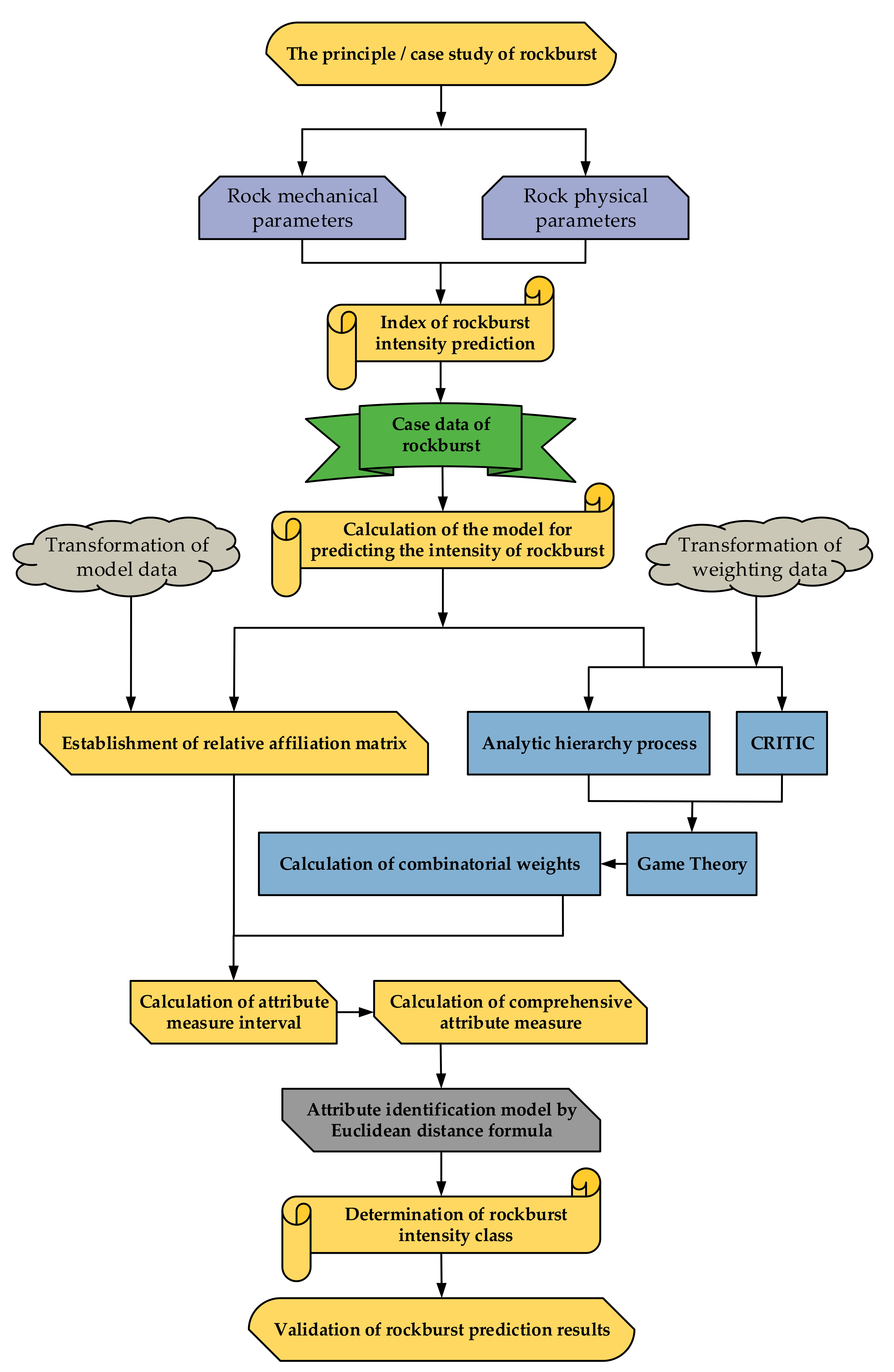
4.1. The Framework of the Model

In this study, the prediction of rockburst intensity is based on game theory and an improved maximum entropy-attribute measure interval model. The overall framework of the model consists of the following main components:

(1)

Studying the mechanism of rockburst occurrence, selecting reasonable indexes for rockburst prediction, and analysing the number field to measure relationships between the indexes and the rockburst class.

(2)

Choosing typical rockburst cases from around the world as the data source for the model study, establishing the measurement relationship between indexes and intensity, and processing the data using the maximum entropy-attribute measurement interval in accordance with the model’s requirements.

(3)

Calculating the subjective weights of the indexes by the Analytic Hierarchy Process method and the objective weights by the CRITIC method based on the data of the case, and proposing the combined weighting method based on game theory, taking into account the subjective advantages and objective advantages.

(4)

Combining the combined weights to calculate the attribute measures of the boundary for the sample and transforming the attribute measures of the boundary into the comprehensive attribute measures of the sample by means of compromise decision coefficient.

(5)

Based on the improved attribute identification mode, the Euclidean distance formula was used to determine the class of intensity for the rockburst. By summarising elements of the model framework, the overall flow of the framework is made as shown in Figure 1.

4.2. Research on the Application of Model

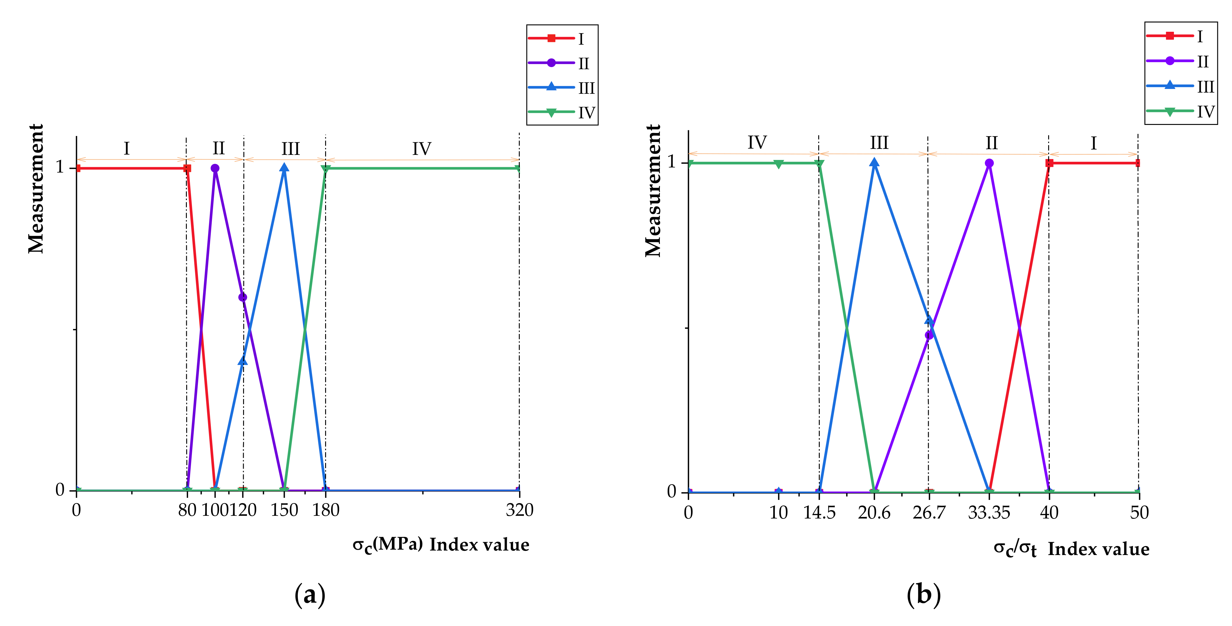
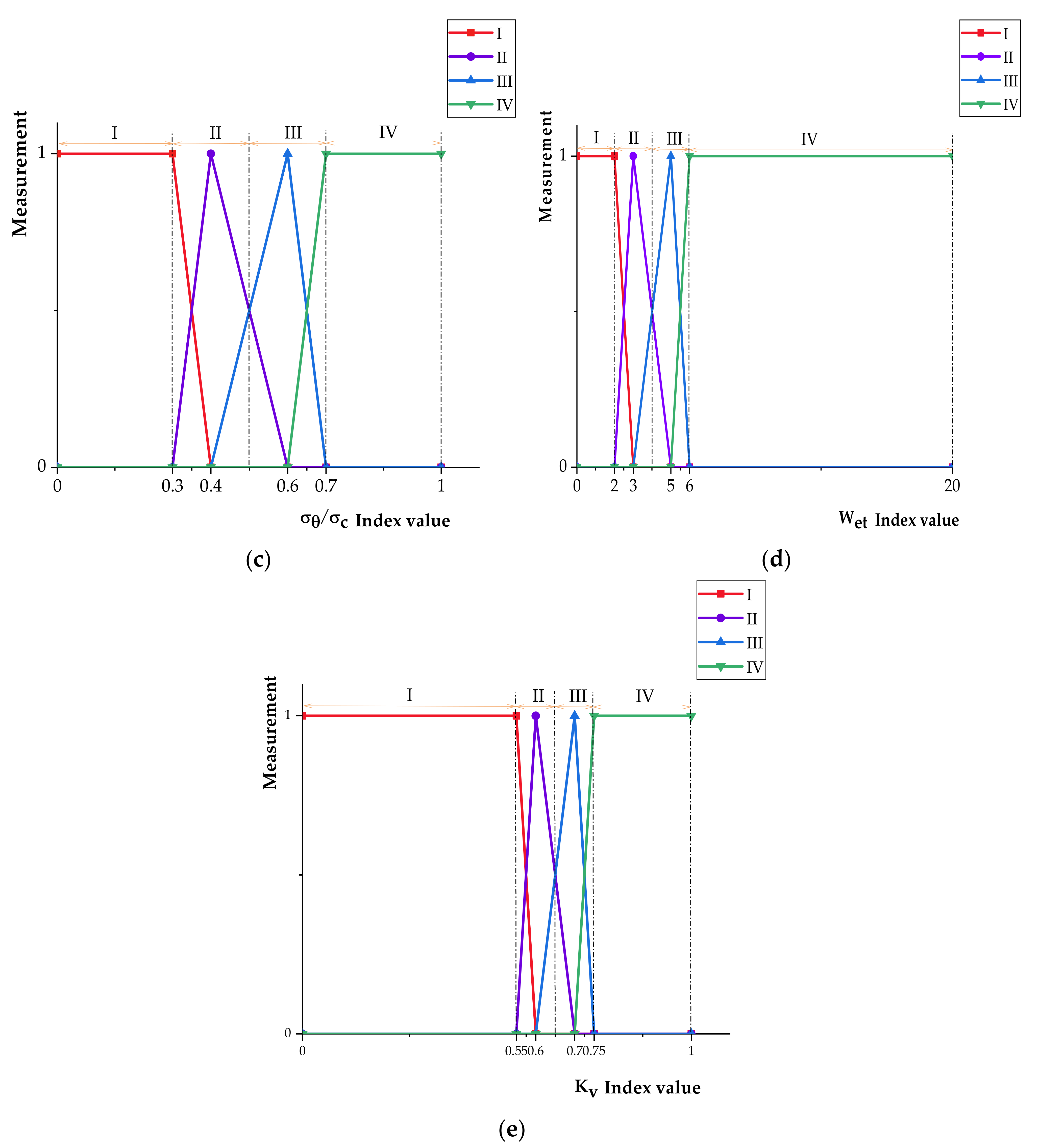
4.2.1. The Indexes of the Rockburst and Intensity Classification Standard

The prediction of rockburst intensity is based on the study of the mechanism of rockburst occurrence. The mechanism and induced conditions for the occurrence of rockburst are still unclear, generally focusing on stress indexes and rock property parameters as the main objects of study. From the many research results [3,4,46,64,65,66,67,68], the stress indexes of rockburst prediction are mainly uniaxial compressive strength of rock ${\sigma }_c$, shear compression ratio of rock ${\sigma }_{\theta }/{\sigma }_c$, compression-tension ratio of rock ${\sigma }_c/{\sigma }_t$, and elastic deformation coefficient of rock $W_{et}$. Rock property parameters are mainly studied for the integrity coefficient of rock $K_v$. In this study, five indexes were selected as indexes for predicting rockburst intensity. By consulting the relevant literature, the single index of rockburst intensity classification criteria are listed as shown in

Table 2. Single index classification standard for rockburst intensity.

Classification	Behavior	${\mathit{\sigma }}_{\mathit{c}}$ [64,65,66,67,68]	${\mathit{\sigma }}_{\mathit{c}}/{\mathit{\sigma }}_{\mathit{t}}$ [64,65,66,67,68]	${\mathit{\sigma }}_{\mathit{\theta }}/{\mathit{\sigma }}_{\mathit{c}}$ [64,65,66,67,68]	${\mathit{W}}_{\mathit{e}\mathit{t}}$ [64,65,66,67,68]	${\mathit{K}}_{\mathit{v}}$ [64,65,66,67,68]
I	No rockburst	0~80	40~50	0~0.3	0~2	0~0.55
II	Low rockburst	80~120	26.7~40	0.3~0.5	2~4	0.55~0.65
III	Medium rockburst	120~180	14.5~26.7	0.5~0.7	4~6	0.65~0.75
IV	Heavy rockburst	180~320	10~14.5	0.7~1.0	6~20	0.75~1.0

, and the single index measurement is shown in Figure 2.

4.2.2. Calculation of Comprehensive Attribute Measures for Case Samples

In order to verify the accuracy of the game theory and improved maximum entropy-attribute measure interval model for predicting rockburst intensity, 20 groups of typical rockburst cases in the world were selected as samples [4,31,32,33,34,35,69,70], and the data of the cases are listed as shown in

Table 3. Actual data for the rockburst intensity index of samples.

Sample	Actual Data for Rockburst Indexes
	${\mathit{\sigma }}_{\mathit{c}}$	${\mathit{\sigma }}_{\mathit{c}}/{\mathit{\sigma }}_{\mathit{t}}$	${\mathit{\sigma }}_{\mathit{\theta }}/{\mathit{\sigma }}_{\mathit{c}}$	${\mathit{W}}_{\mathit{e}\mathit{t}}$	${\mathit{K}}_{\mathit{v}}$
1	148.4	17.5	0.45	5.1	0.68
2	181	21.7	0.42	4.5	0.67
3	150	27.8	0.23	3.9	0.59
4	165	17.5	0.38	4.5	0.56
5	115	23	0.10	4.7	0.52
6	170	15	0.53	6.5	0.7
7	180	21.7	0.39	5	0.73
8	78.7	29.7	0.41	3.3	0.64
9	140	26.9	0.44	5.5	0.78
10	120	18.5	0.81	3.8	0.68
11	115	23	0.10	5.7	0.34
12	82.4	17.5	0.54	6.6	0.61
13	236	28.4	0.38	5	0.58
14	130	19.7	0.38	5	0.69
15	170	15.04	0.53	9	0.82
16	140	17.5	0.77	5.5	0.86
17	175	24.14	0.36	5	0.92
18	180	21.69	0.42	5	0.87
19	180	21.69	0.32	5	0.79
20	130	21.67	0.38	5	0.78

according to the selected indexes for predicting rockburst intensity. Sample 1 was used for model validation, and the calculation process for the remaining 19 groups of samples was consistent with that of Sample 1 and is presented in the analysis of results.

(1)

Construction of the relative affiliation matrix

According to Equation (2) and Table 2, the classification matrix of sample 1 is presented as follows $E$:

$$E=\left[\begin{array}{lllll}\hfill & I\hfill & II\hfill & III\hfill & IV\hfill \\ {\sigma }_c\hfill & \left[0,80\right]\hfill & \left[80,120\right]\hfill & \left[120,180\right]\hfill & \left[180,320\right]\hfill \\ {\sigma }_c/{\sigma }_t\hfill & \left[40,50\right]\hfill & \left[26.7,40\right]\hfill & \left[14.5,26.7\right]\hfill & \left[10,14.5\right]\hfill \\ {\sigma }_{\theta }/{\sigma }_c\hfill & \left[0,0.3\right]\hfill & \left[0.3,0.5\right]\hfill & \left[0.5,0.7\right]\hfill & \left[0.7,1\right]\hfill \\ W_{et}\hfill & \left[0,2\right]\hfill & \left[2,4\right]\hfill & \left[4,6\right]\hfill & \left[6,20\right]\hfill \\ K_v\hfill & \left[0,0.55\right]\hfill & \left[0.55,0.65\right]\hfill & \left[0.65,0.75\right]\hfill & \left[0.75,1\right]\hfill \end{array}\right]$$

(31)

According to the index values of Sample 1 and the single index measure function in Figure 2, the lower boundary standard matrix $A$ and the upper boundary standard matrix $B$ are, respectively, transformed into the corresponding relative affiliation matrices $\underset{¯}{R_1}$ and $\overline{R_1}$ as follows:

$$\underset{¯}{R_1}=\left[\begin{array}{ccccc}& I& II& III& IV\\ {\sigma }_c& 0& 0.44& 0.67& 1\\ {\sigma }_c/{\sigma }_t& 0& 0.44& 0.85& 1\\ {\sigma }_{\theta }/{\sigma }_c& 0& 0.43& 0.71& 1\\ W_{et}& 0& 0.33& 0.67& 1\\ K_v& 0& 0.73& 0.87& 1\end{array}\right] \overline{R_1}=\left[\begin{array}{ccccc}& I& II& III& IV\\ {\sigma }_c& 0& 0.17& 0.42& 1\\ {\sigma }_c/{\sigma }_t& 0& 0.28& 0.66& 1\\ {\sigma }_{\theta }/{\sigma }_c& 0& 0.29& 0.57& 1\\ W_{et}& 0& 0.11& 0.22& 1\\ K_v& 0& 0.22& 0.44& 1\end{array}\right]$$

(32)

Following Equations (6)–(9) and the actual data of the rock burst index for sample 1, the relative affiliation matrices $\underset{¯}{F_1}$ and $\overline{F_1}$ of the actual measured values of sample 1 with respect to the lower boundary standard matrix $A$ and the upper boundary standard matrix $B$ were calculated as follows:

$$\underset{¯}{F_1}=\left[\begin{array}{cc}{\sigma }_c& 0.82\\ {\sigma }_c/{\sigma }_t& 0.75\\ {\sigma }_{\theta }/{\sigma }_c& 0.64\\ W_{et}& 0.85\\ K_v& 0.91\end{array}\right] \overline{F_1}=\left[\begin{array}{cc}{\sigma }_c& 0.29\\ {\sigma }_c/{\sigma }_t& 0.92\\ {\sigma }_{\theta }/{\sigma }_c& 0.21\\ W_{et}& 0.17\\ K_v& 0.29\end{array}\right]$$

(33)

(2)

Combined weights of the indexes

Assuming that the set of indicator values obtained by the AHP method is $W1=\left\{W1.11,W1.12,\dots ,W1.45\right\}$ and the set of indicator values obtained by the CRITIC method is $W2=\left\{W2.11,W2.12,\dots ,W2.45\right\}$, the combination weights can be obtained from Equation (30) as ${\omega }^{*}={\delta }^{*}{}_1{\omega }_1^T+{\delta }^{*}{}_2{\omega }_2^T$, and there is a set of equations reflecting the relationship between the set of indicators and ${\delta }_i$ is as follows:

$$\left\{\begin{array}{l}{\delta }_1{\omega }_1{\omega }_1^T+{\delta }_2{\omega }_1{\omega }_2^T={\omega }_1{\omega }_1^T\\ {\delta }_2{\omega }_2{\omega }_1^T+{\delta }_2{\omega }_2{\omega }_2^T={\omega }_2{\omega }_2^T\end{array}\right.$$

(34)

By calculating this, ${\delta }_1=0.8198$ and ${\delta }_2=0.2064$ are obtained. Normalising ${\delta }_1$ and ${\delta }_2$ results in ${\delta }^{*}{}_1=0.7989$ and ${\delta }^{*}{}_2=0.2011$. The weights of the rock burst indexes are shown in

Table 4. Index weights for rockburst intensity.

Indexes	AHP	CRITIC	Game Theory
${\sigma }_c$	0.112	0.235	0.137
${\sigma }_c/{\sigma }_t$	0.257	0.223	0.250
${\sigma }_{\theta }/{\sigma }_c$	0.221	0.192	0.215
$W_{et}$	0.288	0.168	0.264
$K_v$	0.122	0.182	0.134

.

(3)

Calculation of attribute measurement intervals

The upper boundary attribute measure and lower boundary attribute measure for sample 1 are calculated using Equations (13), (32), and (33):

$$\left.\begin{array}{l}\underset{¯}{{\tau }_{11}}=0.00084\hspace{1em}\overline{{\tau }_{11}}=0.06692\\ \underset{¯}{{\tau }_{12}}=0.07357\hspace{1em}\overline{{\tau }_{12}}=0.40387\\ \underset{¯}{{\tau }_{13}}=0.68162\hspace{1em}\overline{{\tau }_{13}}=0.52041\\ \underset{¯}{{\tau }_{14}}=0.24398\hspace{1em}\overline{{\tau }_{14}}=0.00881\end{array}\right\}$$

(35)

Next, from Equation (14), the comprehensive attribute measure for sample 1 is calculated as follows:

$$\left.\begin{array}{l}{\tau }_{11}=0.03388\\ {\tau }_{12}=0.23872\\ {\tau }_{13}=0.60102\\ {\tau }_{14}=0.12641\end{array}\right\}$$

(36)

4.2.3. Determination of Rockburst Intensity Class

According to the description in Section 2.4, the partition set $C_i$ for each class is set as follows:

$$\left.\begin{array}{l}{C}_1=\left[1,0,0,0\right]\\ C_2=\left[0,1,0,0\right]\\ C_3=\left[0,0,1,0\right]\\ C_4=\left[0,0,0,1\right]\end{array}\right\}=C_i$$

(37)

Then, the results of the Euclidean distance calculation for sample 1 are shown below:

$$\left.\begin{array}{l}{d}_{c_{11}}=\sqrt{{(0.03388-1)}^2+{(0.23872-0)}^2+{(0.60102-0)}^2+{(0.12641-0)}^2}=1.16944\\ d_{c_{12}}=\sqrt{{(0.03388-0)}^2+{(0.23872-1)}^2+{(0.60102-0)}^2+{(0.12641-0)}^2}=0.97872\\ d_{c_{13}}=\sqrt{{(0.03388-0)}^2+{(0.23872-0)}^2+{(0.60102-1)}^2+{(0.12641-0)}^2}=0.48301\\ d_{c_{14}}=\sqrt{{(0.03388-0)}^2+{(0.23872-0)}^2+{(0.60102-0)}^2+{(0.12641-1)}^2}=1.08744\end{array}\right\}$$

(38)

Comparing the distance results for each class yields: $d_{C_{13}}<d_{C_{12}}<d_{C_{14}}<d_{C_{11}}$, therefore the comprehensive attribute measure is closest to Class III, predicting the intensity class for Sample 1 rockburst index conditions to be III.

4.3. Analysis of Results

(1)

Analysis for reasonableness of indexes

According to the weights of the three assignment methods listed in Table 4, the weights of the five indexes reflecting the rock burst intensity are plotted as shown in Figure 3. Analysis of the distribution of the index weights in the graph reveals the following results:

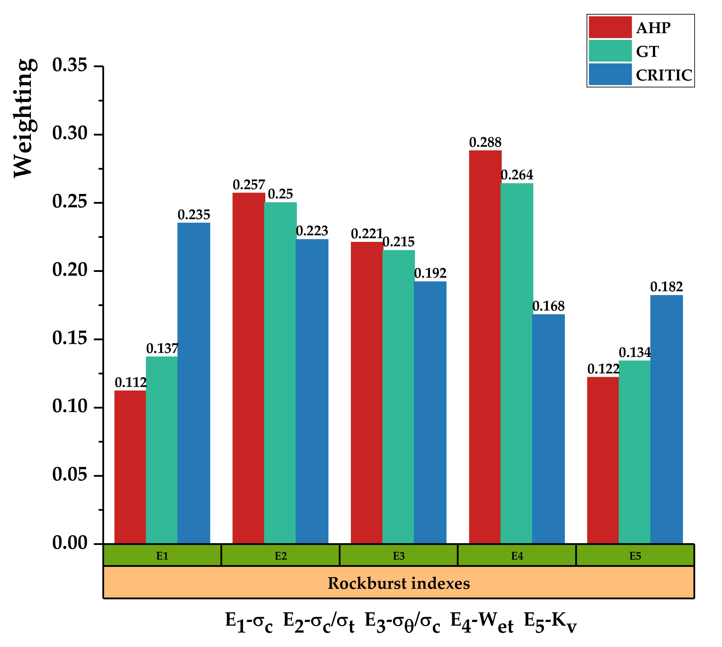
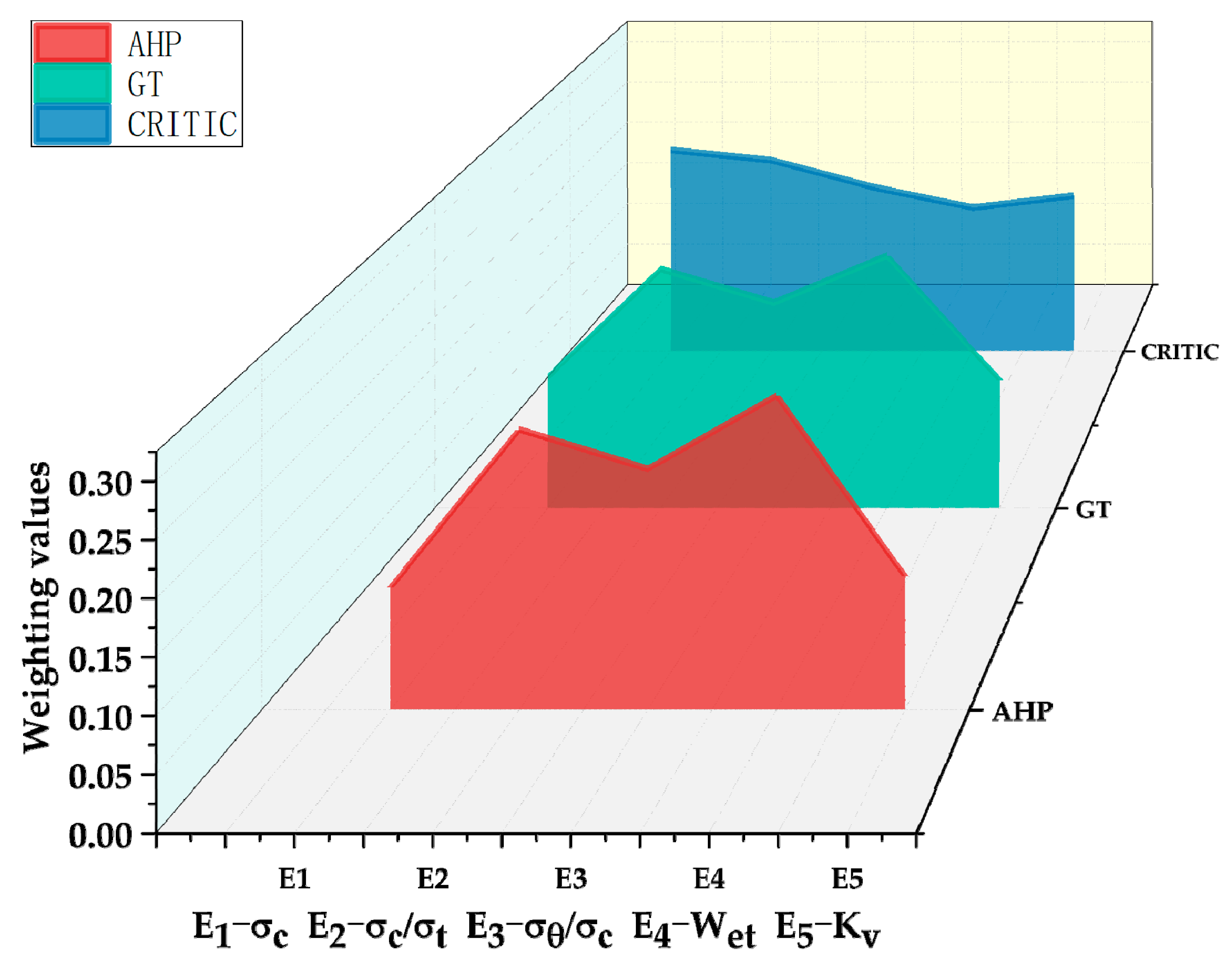
• The difference between subjective weights and objective weights for the same index is large, suggesting that a single weighting method is not scientific in the study of rockburst prediction. This difference could significantly affect the accuracy of the prediction results.
• The different focus of weighting in the Analytic Hierarchy Process and CRITIC methods leads to a significant difference in the extent to which information is used in the weighting process.
• Based on game theory, the combined weights balance the shortcomings of the two single weighting methods, and Figure 4 shows that the overall distribution of the combined weights is more even, taking into account both experts’ experience and objective data information.

(2)

Comparison with other model results

According to the model steps of Sample 1, the remaining 19 sets of rockburst case data are calculated. The game theory and an improved maximum entropy-attribute measure interval model for predicting rockburst intensity (abbreviated in tables and figures as the IME-AMI model) are compared with the fuzzy comprehensive evaluation model result, matter-element extension analysis model result, uncertainty measurement model result, and the actual situation for validation, as shown in

Table 5. Statistics on the predicted result of the case sample.

Sample	Actual Class	Predicted Result (Rockburst Intensity Class)
		IME-AMI Model	Fuzzy Comprehensive Evaluation	Matter-Element Extension Analysis	Uncertainty Measurement Model
1	III	III	III	III	III
2	III	III	III	III	III
3	I	II Δ	II	I	II Δ
4	III	III	Not unique Δ	II Δ	III
5	I	II~III Δ	I	I	II Δ
6	III~IV	III •	III~IV	III •	III~IV
7	III	III	III	III	III
8	II	II	III Δ	III Δ	II
9	III	III	III~IV •	IV Δ	IV Δ
10	III	III	III~IV •	III	III
11	I	III Δ	I	I	I
12	III	III	III~IV •	III	II Δ
13	III	III	III	III	II Δ
14	III	III	III	III	III
15	III	III	III	III~IV •	III
16	III	III	IV Δ	III~IV •	IV Δ
17	III	III	III	III	III
18	III	III	III	No result Δ	III
19	III	III	III	III	III
20	III	III	III	No result Δ	III

In the table, Δ indicates a misjudgement and • indicates an inaccurate judgement.

.

Calculating the accurate judgments, misjudgments, and inaccurate judgments of each model in predicting rockburst intensity is shown in

Table 6. Rockburst prediction situation.

Sample	IME-AMI Model	Fuzzy Comprehensive Evaluation	Matter-Element Extension Analysis	Uncertainty Measurement Model
Accurate (1.0)	16	14	12	14
Inaccurate (0.5)	1	3	3	0
Misjudged (0)	3	3	5	6
Accuracy	80%	70%	60%	70%

. The game theory and an improved maximum entropy-attribute measure interval model for predicting rockburst intensity present better results in terms of accuracy, with 80% accuracy of prediction results for 20 sets of samples; 70% accuracy of prediction results for a fuzzy comprehensive evaluation model; 60% accuracy of prediction results for a matter-element extension analysis model; and 70% accuracy of prediction results for the uncertainty measurement model. The model in this paper has a higher accuracy rate, with more cases accurately judged than other models, and the number of inaccurate and misjudged cases is kept at a low level, indicating that this rockburst intensity model is more accurate and reliable in application. For both inaccurate and misjudged cases, the predicted rockburst results of this model are higher than the actual classes, which means more guaranteed safety if rockburst accidents are prevented according to the predicted results of this model, as shown in Figure 5.

5. Conclusions

(1)

By using the maximum entropy-attribute measure interval model for predicting rockburst intensity, the greyness and ambiguity of index data are eliminated to the greatest extent. Establishing a correspondence between the prediction of rockburst intensity and the partition set of attribute measures, enabling the unification of rockburst prediction and intensity class. Using a compromise decision coefficient integrates the upper and lower boundary of the attribute measure, avoiding the roughness of the numerical interval in the form of the comprehensive attribute measure.

(2)

Starting from the principles of measure theory, the Euclidean distance formula is used to improve the attribute measure recognition mode, and the new measure recognition mode overcomes the shortcomings of the original confidence criterion and improves the accuracy.

(3)

By studying the mechanism of rockburst and typical cases around the world, five indexes (uniaxial compressive strength ${\sigma }_c$, shear compression ratio ${\sigma }_{\theta }/{\sigma }_c$, compression-tension ratio ${\sigma }_c/{\sigma }_t$, elastic deformation coefficient $W_{et}$, and integrity coefficient $K_v$) are identified for the prediction of rockburst intensity. Establishing the measure matrix of indexes and partition set of classes, makes the indexes fit the model better. By balancing the shortcomings of the subjective weights of the Analytic Hierarchy Process and the objective weights of the CRITIC with game theory, the final combined weights take into account the advantages of both types of single index weighting methods.

(4)

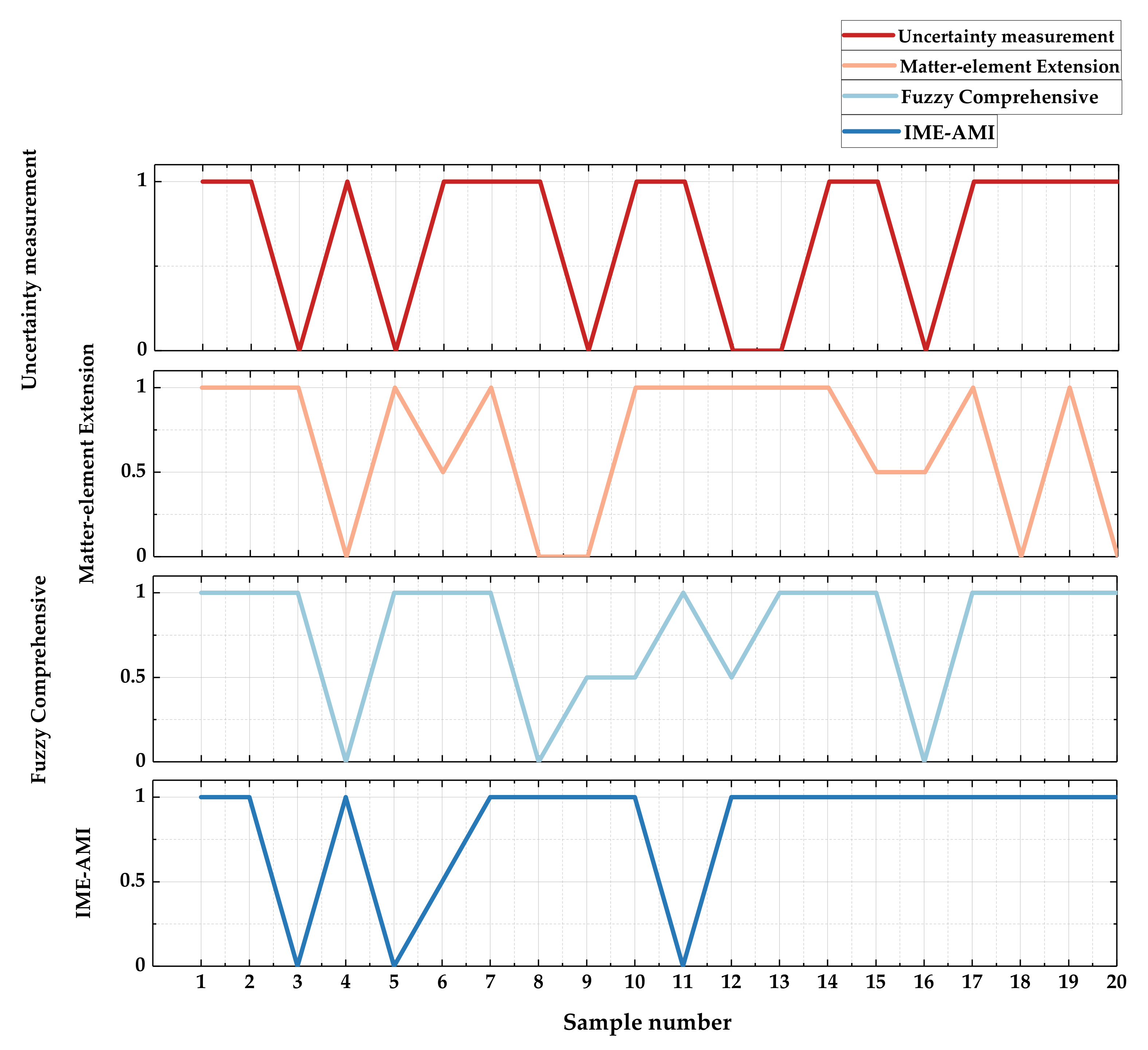
Selecting 20 sets of typical rockburst cases in the world, the results of the game theory and an improved maximum entropy-attribute measure interval model for predicting rockburst intensity are compared with the results of three analytical rockburst prediction models, confirming that the present model is better than the other three models both in terms of accuracy and applicability.

References

1. Cai, W.; Bai, X.; Si, G.; Cao, W.; Gong, S.; Dou, L. A Monitoring Investigation into Rock Burst Mechanism Based on the Coupled Theory of Static and Dynamic Stresses. Rock Mech. Rock Eng. 2020, 53, 5451–5471. [Google Scholar] [CrossRef]
2. Zhao, W.; Qin, C.; Xiao, Z.; Chen, W. Characteristics and contributing factors of major coal bursts in longwall mines. Energy Sci. Eng. 2022, 10, 1314–1327. [Google Scholar] [CrossRef]
3. Yin, X.; Liu, Q.S.; Wang, X.Y.; Huang, X. Prediction model of rockburst intensity classification based on combined weighting and attribute interval recognition theory. Meitan Xuebao/J. China Coal Soc. 2020, 45, 3772–3780. (In Chinese) [Google Scholar] [CrossRef]
4. Wu, S.L.; Yang, S.; Huo, L. Prediction of rock burst intensity based on unascertained measure-intuitionistic fuzzy set. Chin. J. Rock Mech. Eng. 2020, 39, 2930–2939. (In Chinese) [Google Scholar] [CrossRef]
5. Gong, F.Q.; Pan, J.F.; Jiang, Q. The difference analysis of rock burst and coal burst and key mechanisms of deep engineering geological hazards. J. Eng. Geol. 2021, 29, 933–961. (In Chinese) [Google Scholar] [CrossRef]
6. Zhang, W.D.; Ma, T.H.; Tang, C.N.; Tang, L.X. Research on characteristics of rockburst and rules of microseismic monitoring at diversion tunnels in Jinping II hydropower station. Chin. J. Rock Mech. Eng. 2014, 33, 339–348. [Google Scholar] [CrossRef]
7. Feng, G.L.; Feng, X.T.; Xiao, Y.X.; Yao, Z.B.; Hu, L.; Niu, W.J.; Li, T. Characteristic microseismicity during the development process of intermittent rockburst in a deep railway tunnel. Int. J. Rock Mech. Min. Sci. 2019, 124, 104135. [Google Scholar] [CrossRef]
8. Gu, S.; Chen, C.; Jiang, B.; Ding, K.; Xiao, H. Study on the Pressure Relief Mechanism and Engineering Application of Segmented Enlarged-Diameter Boreholes. Sustainability 2022, 14, 5234. [Google Scholar] [CrossRef]
9. Kaiser, P.K.; Moss, A. Deformation-based support design for highly stressed ground with a focus on rockburst damage mitigation. J. Rock Mech. Geotech. Eng. 2022, 14, 50–66. [Google Scholar] [CrossRef]
10. Farhadian, H. A new empirical chart for rockburst analysis in tunnelling: Tunnel rockburst classification (TRC). Int. J. Min. Sci. Technol. 2021, 31, 603–610. [Google Scholar] [CrossRef]
11. Zhou, J.; Li, X.; Mitri, H.S. Evaluation method of rockburst: State-of-the-art literature review. Tunn. Undergr. Space Technol. 2018, 81, 632–659. [Google Scholar] [CrossRef]
12. Afraei, S.; Shahriar, K.; Madani, S.H. Statistical assessment of rock burst potential and contributions of considered predictor variables in the task. Tunn. Undergr. Space Technol. 2018, 72, 250–271. [Google Scholar] [CrossRef]
13. Zhou, J.; Li, X.; Shi, X. Long-term prediction model of rockburst in underground openings using heuristic algorithms and support vector machines. Saf. Sci. 2012, 50, 629–644. [Google Scholar] [CrossRef]
14. Cook, N.G.W. A note on rockbursts considered as a problem of stability. J. South. Afr. Inst. Min. Metall. 1965, 65, 437–446. [Google Scholar]
15. Cook, N.G.W.; Hoek, E.; Pretorius, J.P.; Ortlepp, W.D.; Salamon, H.D.G. Rock mechanics applied to study of rock bursts. J. South. Afr. Inst. Min. Metall. 1966, 66, 435–528. [Google Scholar]
16. Liu, Z.; Shao, J.; Xu, W.; Meng, Y. Prediction of rock burst classification using the technique of cloud models with attribution weight. Nat. Hazards 2013, 68, 549–568. [Google Scholar] [CrossRef]
17. Russenes, B.F. Analysis of Rock Spalling for Tunnels in Steep Valley Sides; Norwegian Institute of Technology: Trondheim, Norway, 1974. [Google Scholar]
18. He, M.; Zhang, Z.; Zhu, J.; Li, N.; Li, G.; Chen, Y. Correlation between the rockburst proneness and friction characteristics of rock materials and a new method for rockburst proneness prediction: Field demonstration. J. Pet. Sci. Eng. 2021, 205, 108997. [Google Scholar] [CrossRef]
19. Chen, X.; Sun, J.; Zhang, J.; Chen, Q. Judgment indexes and classification criteria of rock-burst with the extension judgment method. China Civ. Eng. J. 2009, 42, 82–88. [Google Scholar]
20. Lee, S.M.; Park, B.S.; Lee, S.W. Analysis of rockbursts that have occurred in a waterway tunnel in Korea. Int. J. Rock Mech. Min. Sci. 2004, 41, 911–916. [Google Scholar] [CrossRef]
21. Zhang, J.J.; Fu, B.J. Rockburst and its criteria and control. Chin. J. Rock Mech. Eng. 2008, 27, 2034–2042. [Google Scholar]
22. Shang, Y.J.; Zhang, J.J.; Fu, B.J. Analyses of three parameters for strain mode rockburst and expression of rockburst potential. Chin. J. Rock Mech. Eng. 2013, 32, 1520–1527. [Google Scholar]
23. Sharan, S.K. A finite element perturbation method for the prediction of rock burst. Comput. Struct. 2007, 85, 1304–1309. [Google Scholar] [CrossRef]
24. Jiang, Q.; Feng, X.T.; Xiang, T.B.; Su, G.S. Rockburst characteristics and numerical simulation based on a new energy index: A case study of a tunnel at 2500 m depth. Bull. Eng. Geol. Environ. 2010, 69, 381–388. [Google Scholar] [CrossRef]
25. Lu, A.H.; Mao, X.B.; Liu, H.S. Physical simulation of rock burst induced by stress waves. J. China Univ. Min. Technol. 2008, 18, 401–405. [Google Scholar] [CrossRef]
26. Wang, Y.H.; Li, W.D.; Li, Q.G.; Xu, Y.; Tan, G.H. Method of fuzzy comprehensive evaluations for rockburst prediction. J. Rock Mech. Eng. 1998, 5, 15–23. (In Chinese) [Google Scholar]
27. Qin, S.W.; Chen, J.P.; Wang, Q.; Qiu, D.H. Research on rockburst prediction with extenics evaluation based on rough set. In Proceedings of the 13th International Symposium on Rockburst and Seismicity in Mines, Dalian, China, 21–23 August 2009; pp. 937–944. [Google Scholar]
28. Jiong, W.; Peng, L.; Lei, M.; He, M.C. A Rockburst Proneness Evaluation Method Based on Multidimensional Cloud Model Improved by Control Variable Method and Rockburst Database. Lithosphere 2022, 2021, 5354402. [Google Scholar] [CrossRef]
29. Wang, M.; Liu, Q.; Wang, X.; Shen, F.; Jin, J. Prediction of Rockburst Based on Multidimensional Connection Cloud Model and Set Pair Analysis. Int. J. Geomech. 2020, 20, 04019147. [Google Scholar] [CrossRef]
30. Wang, J.; Huang, M.; Guo, J. Rock Burst Evaluation Using the CRITIC Algorithm-Based Cloud Model. Front. Phys. 2021, 8, 593701. [Google Scholar] [CrossRef]
31. Gong, F.Q.; Li, X.B.; Lin, H. Model of Distance Discriminant Analysis for Rockburst Prediction in Tunnel Engineering and Its Application. China Railw. Sci. 2007, 4, 25–28. (In Chinese) [Google Scholar]
32. Yin, X.; Liu, Q.; Pan, Y.; Huang, X.; Wu, J.; Wang, X. Strength of Stacking Technique of Ensemble Learning in Rockburst Prediction with Imbalanced Data: Comparison of Eight Single and Ensemble Models. Nat. Resour. Res. 2021, 30, 1795–1815. [Google Scholar] [CrossRef]
33. Zhou, J.; Chen, C.; Du, K.; Jahed Armaghani, D.; Li, C. A new hybrid model of information entropy and unascertained measurement with different membership functions for evaluating destressability in burst-prone underground mines. Eng. Comput. 2022, 38, 381–399. [Google Scholar] [CrossRef]
34. Zhou, K.P.; Yun LI, N.; Deng, H.W.; Li, J.L.; Liu, C.J. Prediction of rock burst classification using cloud model with entropy weight. Trans. Nonferrous Met. Soc. China 2016, 26, 1995–2002. [Google Scholar] [CrossRef]
35. Shi, X.Z.; Zhou, J.; Dong, L.; Hu, H.Y.; Wang, H.Y.; Chen, S.R. Application of unascertained measurement model to prediction of classification of rockburst intensity. Chin. J. Rock Mech. Eng. 2010, 29, 2720–2726. [Google Scholar]
36. Chang-Ping, W. Application of attribute synthetic evaluation system in prediction of possibility and classification of rockburst. Eng. Mech. 2008, 25, 153–158. [Google Scholar]
37. Chen, H.J.; Li, X.B.; Zhang, Y. Study on application of set pair analysis method to prediction of rockburst. J. Univ. South China 2008, 22, 10–14. [Google Scholar]
38. Gao, W. Prediction of rock burst based on ant colony clustering algorithm. Chin. J. Geotech. Eng. 2010, 32, 874–880. (In Chinese) [Google Scholar]
39. Chen, B.R.; Feng, X.T.; Li, Q.P.; Luo, R.Z.; Li, S. Rock Burst Intensity Classification Based on the Radiated Energy with Damage Intensity at Jinping II Hydropower Station, China. Rock Mech. Rock Eng. 2015, 48, 289–303. [Google Scholar] [CrossRef]
40. Qin, C.; Zhao, W.; Zhong, K.; Chen, W. Prediction of longwall mining-induced stress in roof rock using LSTM neural network and transfer learning method. Energy Sci. Eng. 2022, 10, 458–471. [Google Scholar] [CrossRef]
41. Cichy, T.; Prusek, S.; Świątek, J.; Apel, D.B.; Pu, Y. Use of Neural Networks to Forecast Seismic Hazard Expressed by Number of Tremors Per Unit of Surface. Pure Appl. Geophys. 2020, 177, 5713–5722. [Google Scholar] [CrossRef]
42. Afraei, S.; Shahriar, K.; Madani, S.H. Developing intelligent classification models for rock burst prediction after recognizing significant predictor variables, Section 1: Literature review and data preprocessing procedure. Tunn. Undergr. Space Technol. 2019, 83, 324–353. [Google Scholar] [CrossRef]
43. Gong, F.Q.; Li, X.B.; Zhang, W. Rockburst prediction of underground engineering based on Bayes discriminant analysis method. Rock Soil Mech. 2010, 31, 370–377. [Google Scholar]
44. Li, D.; Liu, Z.; Armaghani, D.J.; Xiao, P.; Zhou, J. Novel Ensemble Tree Solution for Rockburst Prediction Using Deep Forest. Mathematics 2022, 10, 787. [Google Scholar] [CrossRef]
45. Guo, J.; Guo, J.; Zhang, Q.; Huang, M. Research on Rockburst Classification Prediction Based on BP-SVM Model. IEEE Access 2022, 10, 50427–50447. [Google Scholar] [CrossRef]
46. Liang, W.Z.; Zhao, G.Y. A review of long-term and short-term rockburst risk evaluations in deep hard rock. J. Rock Mech. Eng. 2022, 41, 19–39. (In Chinese) [Google Scholar] [CrossRef]
47. Wang, D.; Zhu, Y. POME-based fuzzy optimal evaluation model of water environment. J. Hohai Univ. 2002, 30, 56–60. (In Chinese) [Google Scholar]
48. Martyushev, L.M. Maximum entropy production principle: History and current status. Physics-Uspekhi 2021, 64, 558–583. [Google Scholar] [CrossRef]
49. Deng, J.; Li, S.; Jiang, Q.; Chen, B. Probabilistic analysis of shear strength of intact rock in triaxial compression: A case study of Jinping II project. Tunn. Undergr. Space Technol. 2021, 111, 103833. [Google Scholar] [CrossRef]
50. Jia, Z.; Zhao, L.; Fan, Z. High-quality substation project evaluation based on attribute measurement interval theory. Power Autom. Equip. 2012, 32, 67–71. (In Chinese) [Google Scholar]
51. Tao, Y.; Xue, Y.; Zhang, Q.; Yang, W.; Li, B.; Zhang, L.; Qu, C.; Zhang, K. Risk Assessment of Unstable Rock Masses on High-Steep Slopes: An Attribute Recognition Model. Soil Mech. Found. Eng. 2021, 58, 175–182. [Google Scholar] [CrossRef]
52. Xu, Z.; Cai, N.; Li, X.; Xian, M.; Dong, T. Risk assessment of loess tunnel collapse during construction based on an attribute recognition model. Bull. Eng. Geol. Environ. 2021, 80, 6205–6220. [Google Scholar] [CrossRef]
53. Chen, S.Y.; Yu, X.F. Relative membership grade theory and its application in assessing groundwater quality. J. Liaoning Univ. Eng. Technol. 2003, 22, 691–694. (In Chinese) [Google Scholar]
54. Zou, Q.; Zhou, J.; Zhou, C.; Chen, S.; Song, L.; Guo, J.; Liu, Y. Flood disaster risk analysis based on principle of maximum entropy and attribute interval recognition theory. Adv. Water Sci. 2012, 23, 323–333. (In Chinese) [Google Scholar] [CrossRef]
55. Qin, S.W.; Lv, J.F.; Chen, J.P.; Chen, J.J.; Ma, Z.J.; Cao, R.G.; Liu, X.; Zhai, J.J. Risk evaluation of mountain tunnel collapse based on maximum entropy principle and attribute interval recognition theory. People’s Changjiang 2017, 48, 91–96. (In Chinese) [Google Scholar] [CrossRef]
56. Zhou, X.W.; Wang, L.P.; Zhang, C.K. A Fuzzy Assessment Model Based on Maximum Entropy for River Water Quality Recoverability. China Rural Water Conserv. Hydropower 2008, 1, 23–25. (In Chinese) [Google Scholar]
57. Xiao, H.; Wang, M.; Xi, X. A Consistency Check Method for Trusted Hesitant Fuzzy Sets with Confidence Levels Based on a Distance Measure. Complexity 2020, 2020, 9762695. [Google Scholar] [CrossRef]
58. Aggarwal, E.; Mohanty, B.K. An Algorithmic-based Multi-attribute Decision Making Model under Intuitionistic Fuzzy Environment. J. Intell. Fuzzy Syst. 2022, 42, 5537–5551. [Google Scholar] [CrossRef]
59. Saaty, T.L.; Kearns, K.P. The analytic hierarchy process. In Analytical Planning: The Organization of System; Pergamon Press: Oxford, UK, 1985. [Google Scholar]
60. Vashishtha, S.; Ramachandran, M. Multicriteria evaluation of demand side management (DSM) implementation strategies in the Indian power sector. Energy 2006, 31, 2210–2225. [Google Scholar] [CrossRef]
61. Mir, M.A.; Ghazvinei, P.T.; Sulaiman, N.M.N.; Basri, N.E.A.; Saheri, S.; Mahmood, N.Z.; Jahan, A.; Begum, R.A.; Aghamohammadi, N. Application of TOPSIS and VIKOR improved versions in a multi criteria decision analysis to develop an optimized municipal solid waste management model. J. Environ. Manag. 2016, 166, 109–115. [Google Scholar]
62. Opricovic, S. Multicriteria optimization of civil engineering systems. Fac. Civ. Eng. Belgrade 1998, 2, 5–21. [Google Scholar]
63. He, H.; Xing, R.; Han, K.; Yang, J. Environmental risk evaluation of overseas mining investment based on game theory and an extension matter element model. Sci. Rep. 2021, 11, 16364. [Google Scholar] [CrossRef]
64. Gong, F.; Wang, Y.; Wang, Z.; Pan, J.; Luo, S. A new crition of coal burst proneness based on the residual elastic energy index. Int. J. Min. Sci. Technol. 2021, 31, 11. [Google Scholar] [CrossRef]
65. Wu, G.S.; Yu, W.J.; Zuo, J.P.; Li, C.Y.; Li, J.H.; Du, S.H. Experimental investigation on rockburst behavior of the rock-coal-bolt specimen under different stress conditions. Sci. Rep. 2020, 10, 7556. [Google Scholar] [CrossRef] [PubMed]
66. Shukla, R.; Khandelwal MKankar, P.K. Prediction and Assessment of Rock Burst Using Various Meta-heuristic Approaches. Min. Metall. Explor. 2021, 38, 1375–1381. [Google Scholar] [CrossRef]
67. Li, Z.; Xue, Y.; Li, S.; Qiu, D.; Zhang, L.; Zhao, Y.; Zhou, B. Rock burst risk assessment in deep-buried underground caverns: A novel analysis method. Arab. J. Geosci. 2020, 13, 388. [Google Scholar] [CrossRef]
68. Yang, Y.; Zhu, J. A new model for classified prediction of rockburst and its application. Mei T’an Hsueh Pao (J. China Coal Soc.) 2000, 25, 169–172. [Google Scholar]
69. Guo, J.; Zhang, W.X.; Zhao, Y. A multidimensional cloud model for rockburst prediction. Chin. J. Rock Mech. Eng. 2018, 37, 1199–1206. (In Chinese) [Google Scholar]
70. Bai, Y.F.; Deng, J.; Dong, L.J.; Li, X. FDA model of rock burst prediction and its application in deep hard rock engineering. Chin. J. Cent. South Univ. Sci. Technol. 2009, 40, 1417–1422. (In Chinese) [Google Scholar]
Figure 1. Model framework for predicting rockburst intensity.
Mathematics 10 02551 g001
Figure 2. Single index measurement function for rockburst. (a) Measurements of rock uniaxial compressive strength. (b) Measurements of rock compres-sion-tension ratio. (c) Measurements of rock shear compression ratio. (d) Measurements of rock elastic deformation coefficient. (e) Measurements of rock integrity coefficient.
Mathematics 10 02551 g002aMathematics 10 02551 g002b
Figure 3. Index weight distribution of rockburst intensity.
Mathematics 10 02551 g003
Figure 4. Visual comparison of index weights.
Mathematics 10 02551 g004
Figure 5. Comparison of prediction results of different models.
Mathematics 10 02551 g005