
Theoretical Bounds on the Number of Tests in Noisy Threshold Group Testing Frameworks

Department of Convergence Software, Mokpo National University, Muan 58554, Korea
Mathematics 2022, 10(14), 2508; https://doi.org/10.3390/math10142508
Submission received: 9 June 2022
/
Revised: 15 July 2022
/
Accepted: 15 July 2022
/
Published: 19 July 2022
(This article belongs to the Special Issue Probability and Stochastic Processes with Applications to Communications, Systems and Networks)
Abstract
:We consider a variant of group testing (GT) models called noisy threshold group testing (NTGT), in which when there is more than one defective sample in a pool, its test result is positive. We deal with a variant model of GT where, as in the diagnosis of COVID-19 infection, if the virus concentration does not reach a threshold, not only do false positives and false negatives occur, but also unexpected measurement noise can reverse a correct result over the threshold to become incorrect. We aim to determine how many tests are needed to reconstruct a small set of defective samples in this kind of NTGT problem. To this end, we find the necessary and sufficient conditions for the number of tests required in order to reconstruct all defective samples. First, Fano’s inequality was used to derive a lower bound on the number of tests needed to meet the necessary condition. Second, an upper bound was found using a MAP decoding method that leads to giving the sufficient condition for reconstructing defective samples in the NTGT problem. As a result, we show that the necessary and sufficient conditions for the successful reconstruction of defective samples in NTGT coincide with each other. In addition, we show a trade-off between the defective rate of the samples and the density of the group matrix which is then used to construct an optimal NTGT framework.
MSC:
68Q011. Introduction
Group Testing (GT) is a underdetermined problem in [1], and numerous methods have been developed to solve their problems. GT has become relevant in various problems including probabilistic approaches. The expansion of compressive sensing goes back to the fundamental idea of GT because it is an effort to find sparse signals [2,3]. Recently, academia has begun using the GT method as on vital approach to finding confirmed COVID-19 cases, showing this field’s potential importance in these uncertain times [4,5].
The first study for GT was proposed by Dorfman [1]. The background to the emergence of GT is that a large project was conducted in the United States to find soldiers with syphilis during World War II. Syphilis testing of inviduals involves taking a blood sample, then analyzing that to produce a positive or negative result for syphilis in that patient. The syphilis testing carried out at the time was very inefficient since it took a lot of time and money to test all the soldiers one by one [3]. After all, if N soldiers are individually tested for syphilis, N tests are required. Note that the number of soldiers infected with syphilis is very small compared to the total number of soldiers. That is why it is probably inefficient to test every soldier for syphilis one by one, and why the GT technique emerged. The initial GT model was performed in the following way [1]. Several soldiers’ blood samples were randomly selected, and the blood was put into a pool and mixed. Then, the blood pool was checked to see if it activated to syphilis or not. A positive result indicates that at least one of the soldiers in the pool was infected with syphilis. A negative result, on the other hand, indicates that all soldiers in the pool were free of syphilis. GT is attractive because the number of tests can be drastically reduced in the case of fewer soldiers infected with syphilis. After these beginnings, GT has mainly been studied with two different approaches, each forming a field of research of its own. One these fields is how to generate GT models. That is, it is a method of selecting samples to be included in one test pool. The second area is to reconstruct defective samples with as few tests as possible. GT loses its benefits if the requirement for a large number of retests leads to as many tests as the number of tests for individual screening.
For GT, various models have been proposed in consideration of how the test results express positive and negative results and the presence or absence of noise. In general, GT’s test results told us to see if the pool under being tested contains one or more defective samples. That is, a positive or negative result indicates whether at least one of the defective samples in the pool are present. The model called quantitative GT [3] is a generalization framework of GT. The test result of quantitative GT indicates the number of defective samples in the test pool. There is also another GT model called Threshold Group Testing (TGT) [6]. In the TGT model, a test result of a pool is positive or negative as in conventional GT schemes. However, unlike the conventional GT model, the positive result occurs only when the number of defective samples in the pool is greater than a given threshold. Otherwise, the test outcome is negative. The TGT model is used because it can represent situations in which the test result can be different depending on whether it is high or low, such as the COVID-19 virus concentration. A modified GT model in which measurement noise causes false negatives or false positives is also considered.
TGT problems have been dealt with in various fields such as construction of TGT models [7], theoretical analysis of performance [8], and efficient model design [9,10]. However, there have been no studies so far to quantify how much measurement noise affects performance of TGT models. In this paper, we consider a Noisy Threshold Group Testing (NTGT) model. We provide guidelines for designing a NTGT model that is robust and reliable to measurement noise. To this end, a lower bound on the number of tests is derived using Fano’s inequality. We show the trade-off relationship between the sparsity of the group matrix and the defective rate of the signal. And we obtain an upper bound on the probability of an error using the MAP decoding method. We show necessary and sufficient conditions on the number of tests required for finding a set of given defective samples using the lower and upper bounds.
2. Related Work
We look through previous studies and their significance to GT. Then, we will classify each type of problem related to current approaches to GT and consider the issues surrounding these problems. The study of GT first began in 1943 [1]. Dorfman made an effort to find a small number of syphilis-infected soldiers. Dorfman performed the GT with the following procedure. When testing for syphilis, all the soldiers were divided into various groups that were equal in size, then individual testing was only performed on soldiers from the groups that had recoded positive test results. In [1], the optimal group size for a given total number of samples and defective rate was summarized and presented. Later, Sterrett improved the performance by slightly modifying the existing GT method [11]. The main idea of Sterrett’s approach is that once the first positive result is obtained, the remaining untested individuals are put in one large grouped and tested. Other than that, there is no difference between Sterrett’s method and Dorfman’s. If there is a low infection rate, Sterrett’s method is more efficient because most of the samples are normal. A more general GT has been presented in [12], in which several algorithms were developed for finding defective samples when no infection rate exists. The paper [12] also provided a link between information theory and GT, introduced a new application of GT, and discussed the generalization of GT.
GT is classified based on types of defective sample distributions and decoding approaches. A probabilistic model uses the assumption that a defective sample is generated from a given probability distribution. On the other hand, the combinatorial model is an attempt to find defective samples without knowledge of probability distributions [13,14]. A typical example of this model is the minmax algorithm [15]. In [16], the results of improved performance in the combinatorial model were presented. Looking at other classes, the adaptive case is a model in which samples to be included in one pool are not independent of the results of previous tests. The samples to be used for the next round are changed each time based on the results of previous tests. Specifically, the method of selecting samples to be included in the next pool is optimized by using the results obtained from previous tests. Conversely, in the non-adaptive model, all tests are performed at the same time by a sample selection process defined in advance. So in this model, every test is independent of each other. This model offers the advantage of being able to test simultaneously regardless of the test order. When predetermined multiple steps are used, the non-adaptive model is extended to multi-stage models [1,17]. In fact, although the adaptive model has more constraints in GT design than the non-adaptive model, the adaptive model generally outperforms the non-adaptive model [3]. However, the recent research in [18] showed limitations in improving the performance of the adaptive model. Non-adaptive GTs are more efficient if all tests are being performed at the same time.
We now look at the significance of certain recent studies on noisy GT. The work in [19] showed the information-theoretic performance of GT with and without measurement noise. Several studies have recently showed interesting and significant performance. In [17], the proposed algorithms uses positive rates in the group to be included for each sample. In this case, if it is greater than the set value, the sample is considered as defective. This approach does not lead to optimal performance in all domains, but it follows a scaling law for a specific domain. In [19], there is separate testing for signals, and all of the group testing is carried out while still considering each sample. That is, although no individual testing is performed, samples use a binary value such as positive or negative. In the case of samples affected by symmetric noise, it was shown that the minimum number of tests reduces to a proportional to of the optimal information-theoretic bounds for identifying any K defectives samples in a population of N samples [19].
In [20,21], for noisy addition, GT algorithms were presented using message passing and linear programming. Although it does not guarantee optimal performance for decoding complexity, the algorithm proposed in [22] is capable of realistic runtime in terms of that case of a large population. Although many studies have been performed on the noiseless version of GT models, it has been considered as an assumption that the test results are always pure. But this is not realistic. In addition, most of the noisy GT approaches to deal with measurement noise were performed by considering the symmetric noise model such as binary symmetric channel mentioned in channel coding theory. The symmetric noise model referred to in this paper assumes that the test results have the same probability of occurrence of false negatives and false positives. However, asymmetric noise models are more natural than symmetric ones in various applications. For example, data forensics in [23] is an example of using noisy GT models where it identifies to see if recoded files are changed.
3. Noisy Threshold Group Testing Framework
3.1. Problem Statement
We define our NTGT problem. Let be the input expressed as a binary vector of size N, , . For , is the i-th element of . is expressed in binary to identify either a defective sample or a normal sample. In other words, if the i-th sample is defective, , otherwise . Throughout this work, we assume that has the following probability,
where is the defective sample rate, and is a dummy variable. In this case, the defective sample rate is less than 0.5, 0 0.5, which is considered a small value for GT problems.
As mentioned earlier, one of the key points in the GT problems is to determine which samples to participate in a pool. In this paper, samples to be included in the pool are selected using a non-adaptive model. We use a matrix as a more concise way to define the samples to be included in the pool. Let be the group matrix which has M rows and N columns as denoted , where M is the number of tests in the NTGT model. Note that we aim for a small M as the number of tests required to reconstruct the signal . When the j-th test includes i-th sample and performs GT, it is expressed as . Otherwise, . Whether i-th sample is included in the j-th test and performs GT, is expressed as a binary value, i.e., 0 or 1, of each element of the group matrix. Although the d-Separable matrix and the d-Disjunct matrix [3] were used to design the group matrix, the approach of randomly selecting the elements of the group matrix is also known to be a good design method [3]. For and , is identically independent distributed as follows:
where denotes the sparsity of the group matrix and the range of is . As increases, the density of the group matrix also increases. Conversely, as they get smaller, increasingly sparse group matrices are designed. It should be noted that the computational complexity of the GT framework also increases when a group matrix is constructed from a large . Therefore, it is necessary to design GT frameworks with as low as possible the sparsity of group matrices while improving the reconstruction performance. We will consider how the relationship between and affects the number of tests for signal reconstruction.
The reason we are considering the NTGT model is as follows. Consider a model that could be used for the diagnosis of COVID-19 infection. There are cases in which the COVID-19 test showed false positive or false negative results when the concentration of the virus was low or contaminated. The current diagnosis of COVID-19 infection is positive when the virus concentration is above a certain level. During the incubation period or early stage of infection, the virus concentration is low, and false negative results may be obtained. In addition, even if the COVID-19 infection is confirmed using a precise and accurate diagnostic method, the result is sometimes reversed due to unexpected measurement noise. Throughout this work, a NTGT model suited to these challenges is considered. In other words, we consider the best approach to a TGT scheme where positive and negative cases occur by the quatitative concentration, and we consider an additive noise model because measurement noise can reverse the results. In a recent study [24], for the diagnosis of COVID-19 infection, false positives and false negatives were reported to be between 0.1% and 4.5%, respectively. Next, we obtain lower and upper performance bounds on the NTGT model in Section 4 and Section 5.
TGT is different from conventional GT models. In conventional GT, if at least one defective sample exists in one test, the output is positive without measurement noise. However, TGT is positive when there is a number of defective samples greater than the predefined threshold T. For example, means that a positive result occurs only when there are at least three defective samples in the pool. Once there is only one defective sample in the pool, its result would be negative. In other words, the result in the pool becomes positive only when it is above T for TGT models, also whether it is negative or positive in the diagnosis of COVID-19 infection depends on whether the virus concentration is high or low. The conventional GT uses . The following (3) presents an output for a TGT model. Let be the result of the j-th test pool, which does not suffer from noise, where indicates a positive result and 0 for a negative result, , .
Through this paper, we consider the NTGT framework with measurement noise. Assume a model whose results can be flipped due to the measurement noise. is the pure result of the pool test, and its result converts from positive to negative and vice versa due to additive noise. For the NTGT model, the additive noise is defined as follows:
where is the measurement noise, and we assume all are independent of each other. Therefore, the j-th output in the NTGT model can be written as
where the symbol ⊕ denotes the logical operation XOR. We denote and .
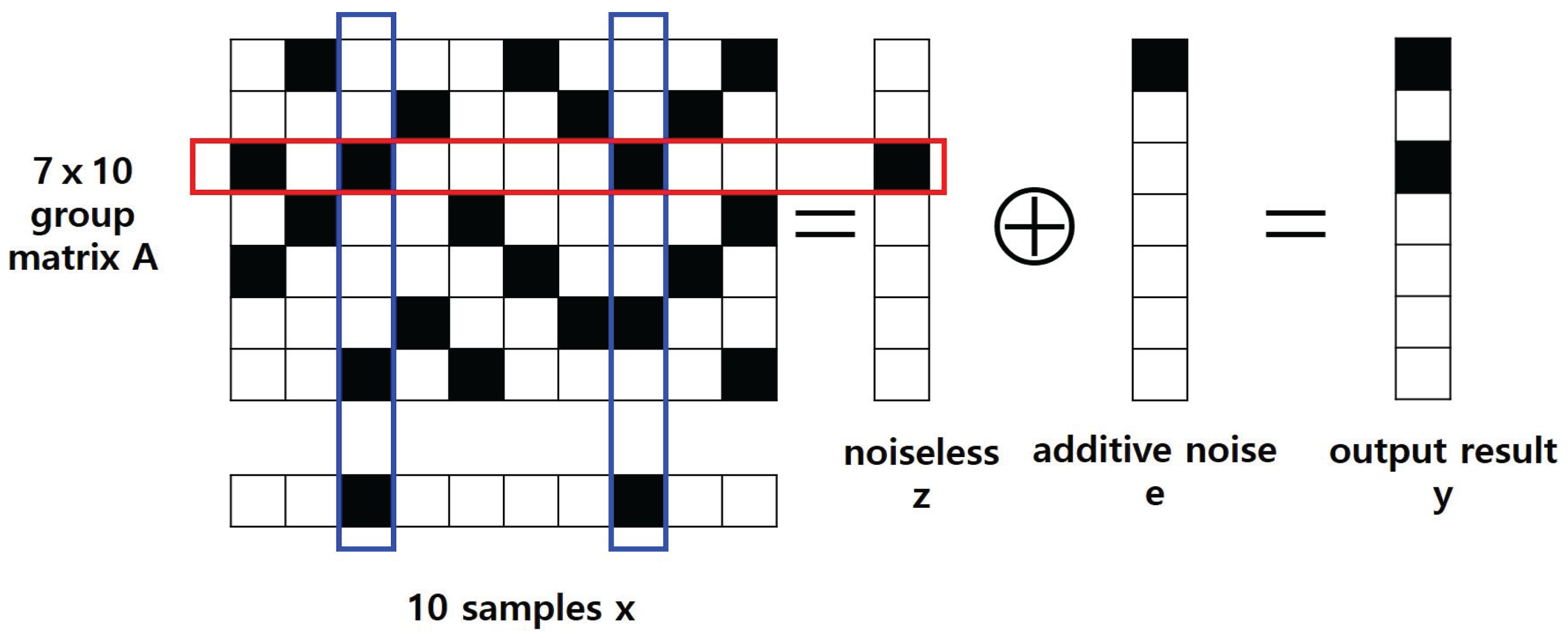
Figure 1 shows an example of this NTGT. In this example, two samples out of ten are defective, which is realized from (1). As shown in Figure 1, the number of tests is 7, . The group matrix is constructed by (2) mentioned above. For noiseless version, the vector is with . In the third test only, the number of defective samples becomes two, and the test result is positive. When additive noise is added as defined in (4), the output is .
3.2. Decoding
We use a maximum a posteriori (MAP) method to reconstruct a signal in the NTGT.
The posteriori probability in (6) is as follows:
The last line of (7) is obtained using independent conditions, while the conditional probability is an indicator function that satisfies the following condition:
We define an error event if from (6) is not the same as the true realization of . In other words, the probability of an error is expressed as .
3.3. Bounds for Group Testing Schemes
Now consider the number of tests on successful decoding in the conventional GT models. The number of tests required to identify K defective samples out of all N samples for an adaptive GT algorithm with perfect reconstruction denotes as . Moreover, for the case of a non-adaptive model, the number of tests is defined as . The number of tests N required for individual testing is greater than . Adaptive GT models require less or equal number of tests than those of non-adaptive GTs because they check the results of previous tests and perform the next tests, . Even if the number of defective samples is one, at least one test must be performed, . Therefore, the number of tests has a wide range as follows:
From an information-theoretic bound, the minimum number of tests M for a GT framework with a sample space is obtained as [3],
where denotes the sample space. In addition, an information-theoretic performance is presented even for a GT framework with small error probability. It is expressed as an upper bound of the error probability for the number of tests required for successful decoding. This GT algorithm performs in such a way as the following bound on successful probability for decoding of defective samples [25]:
In the past half century, many studies on GT models have been performed, and among them, well-known and important GT algorithms are introduced next. The first one to be considered is the binary splitting algorithm [3]. This algorithm solves the existing GT problems efficiently and is applicable to the adaptive GT models. So far, the reason this algorithm is used for GT problems is because of its simplicity and good performance. The number of tests required to reconstruct defective samples using the binary splitting algorithm is known through the following bounds:
where is the number of samples to be included for one test, and p is a uniquely determined nonnegative integer conditioning .
Next, the definite defectives algorithm [26] is considered. This algorithm is suitable for non-adaptive GT models because an unknown input signal can be reconstructed using all of the test results at the same time through an iterative process. The feature of the definite defectives algorithm is attractive in that it can eliminate false negatives that may occur during the reconstruction process. As a result, the use of the definite defectives algorithm is more useful in applications where false negatives are sensitive or should not be present. For given N and K, the definite defective algorithm has the following lower bound for the number of tests M required for identifying defective samples if it is allowed an error rate of ,
4. Necessary Condition for Complete Recovery
4.1. Lower Bound
In this section, we take into account a necessary condition for the number of tests required to identify defective samples in the NTGT model. We obtain the necessary condition using Fano’s inequality theorem [27] presented in information theory. Fano’s inequality is mainly exploited in channel coding theory, and describes the connection between error probability and entropy. In addition, in [28], the authors reviewed GT problems comprehensively and in-depth from an information theory perspective. The lower bound on the probability of an error is obtained by considering Fano’s inequality theorem. From this lower bound, we are lead to the necessary condition for the number of tests to find all defective samples for the NTGT model. We first explain Fano’s inequality theorem before deriving the necessary condition.
Theorem 1
(Fano’s inequality [27]). Suppose there are random variables A and B of finite size. If the decoding function Φ that finds A by considering B is used, the following inequality holds:
where is the probability of an error for the decoding function Φ, and the conditional entropy is defined as follows:
where and are the joint probability and conditional probability, respectively.
In the NTGT problem, we are able to obtain a lower bound on the probability of an error. This lower bound shows the minimum number of tests required to reconstruct an unknown signal, regardless of which decoding function is used. In this paper, our lower bound is a variant of the results obtained in [8]. Compared to [8], this work obtains the lower bound taking into account the measurement noise. However, the overall procedure of derivation is similar to each other because it uses Fano’s inequality theorem.
Theorem 2
Proof of Theorem 2.
Let be the estimated signal of found using the decoding function. Considering the following process in terms of a Markov chain, we can say . Then, the following inequality is satisfied,
Further, from Fano’s inequality described in (14), the conditional entropy is bounded by
Then, the probability of error is bounded in terms of the conditional entropy and the total number of samples N,
It needs to tackle the conditional entropy . Let us divide and expand the following conditional entropy in more detail:
where is mutual information, and equality (a) comes from the fact that and are independent of each other. Note that the smaller the term on the right side of (19), the lower the minimum value of the probability of error. This means that the conditional entropy, , should be small as possible. As a result, on the last line of the right side in (20), the conditional entropy should be large; conversely, the conditional entropy should be small.
To do this, let us find the maximum and minimum values of the two conditional entropies, respectively.
where the first inequality is due to the definition of conditional entropy, and the last inequality comes from the fact that the result is either 0 or 1, values are independent of each other, and the maximum binary entropy is 1 in the case that . Next, we take into account the other conditional entropy which is minimized,
where the second equality comes from how the randomness of vanishes if and are known, the last equality being due to the independent events of . Using (21) and (22), (20) can be rewritten as
Finally, if (19) is changed to satisfy the condition where is a small, positive value and , the following condition holds:
This completes the proof of Theorem 2. □
4.2. Construction of Noisy Threshold Group Testing
We now consider the result obtained from Theorem 2. First, Theorem 2 can be expressed as the ratio of the number of tests to the total number of samples as follows:
It is advantageous to use the NTGT framework until the point N and M are equal. Otherwise, when , individual testing becomes more effective than GT. This shows that NTGT can theoretically be used under the following noise conditions:
To design an NTGT framework, how to construct a group matrix is important. The key to this is shown in the proof of Theorem 2. Looking carefully at the conditions under which the inequality of conditional entropy holds in (21), the maximum conditional entropy is obtained when the following conditions are satisfied: . This means that the NTGT system should be designed so that the output has an equal probability of being 0 or 1. Since and are independent of each other, the probability of an output of 0 is as follows:
As shown in (27), it can be seen that there is a trade-off between and . In other words, to reconstruct a sparse signal, a high-density group matrix needs to be generated and used. Conversely, if the signal is not sparse, the group matrix should be designed with low density.
5. Sufficient Condition for Average Performance
5.1. Upper Bound
Now we prove there is an upper bound on the probability of errors from the MAP decoding used in NTGT. We divide the proof of the upper bound into two parts: one considers the definition of the error event and the other part formulates the probability of errors.
We rewrite the a posteriori probability.
Note that both and are given and known. Using MAP decoding, we estimate with (28)
An error event occurs if there is a feasible vector , such that
where comes from (3), and comes from a realization from (4). When given , , and , we have one vector , such that . Then we can rewrite (30).
Therefore, an error event becomes equivalent to there existing a pair such that
So far, we have defined the error event and now we will derive an upper bound on the probability of error. When given and , we let be the conditional error probability. We have an average error probability as follows:
We now introduce two typical sets that were defined in [27] (Ch.3.1). Let and be typical sets of and with respect to and as defined in (1) and (4). For any positive number and sufficiently large numbers of N and M, the two typical sets are defined as
and
Now we define the space of the pair with respect to the two typical sets. Let and be the sets for the pair such that
and
where is the joint typical set for the pair , since and are independent.
Theorem 3
Proof of Theorem 3.
The probability of error is bounded as
where (a) is due to , and (b) comes from the following,
This is because is randomly generated as defined in (2); then we can define the following event as
The conditional error probability is the probability of the union of all the events in (43) with respect to all pairs that satisfy (32). Thus, the conditional error probability in (33) can be rewritten as
Using the union bound in (41), we have the following bound:
where is the indicator function, such that .
The indicator function is bounded [29] (Ch. 5.6) for .
For in (47), we have the following bound:
In (50), we find the following probability depending on the number of nonzero elements and :
where each row is independent. Given this, we define the following probability:
We can divide in (52) into two parts. If ,
Otherwise,
where
The maximum for by looking at and from the fact that in (54) is concave with respect to and . Therefore, its bound is
As the probability of error is less than 1, the exponent term on the right side of (57) is bounded by
Then, the ratio of M to N is
This completes the proof of Theorem 3. □
5.2. Discussion for Necessary and Sufficient Conditions
In this section, we discuss the results obtained from Theorems 2 and 3. The result from Theorem 2 allows us to solve the lower bound in the NTGT problem using Fano’s inequality. The minimum number of tests required to recover all defective samples with probability out of N samples is also obtained. In other words, Theorem 2 is a necessary condition for any probability of error to be smaller than . Conversely, Theorem 3 leads to the upper bound on the probability of an error using the MAP decoding method. This condition refers to the upper bound on performance and is the sufficient condition to allow us to reconstruct defective samples.
We show that the results of Theorems 2 and 3 coincide with each other. Finding and presenting the necessary and sufficient conditions for the number of tests required in the NTGT problem is significant for TGT. In addition, as shown in (27) above, a system design method for NTGT was proposed so that the probability that a test result is 0 and the probability that it is 1 are the same depending on threshold T.
6. Conclusions
In this paper, we considered a NTGT problem where the test result is positive when the number of defective samples in a pool equals or greater than a certain threshold. Recently, when performing GT for the diagnosis COVID-19 infection, if the sample’s virus concentration did not sufficiently reach the threshold, false positives or false negatives can occur, so in this work we dealt with this TGT framework. In addition, a noise model was added in case pure results were flipped due to unexpected measurement noise. We took into account how many tests were needed to successfully reconstruct a small defective sample with the NTGT problem. To this end, we aimed to find the necessary and sufficient conditions for the number of tests required. For the necessary condition, we obtained the lower bound on the number of tests using Fano’s inequality theorem. Next, the upper bound on performance defined by the probability of error was derived using the MAP decoding method. This result leads to the sufficient condition for identifying all defective samples in the NTGT problem. In this paper, we have shown that the necessary and sufficient conditions are consistent with the NTGT framework. In addition, we presented that the relationship between the defective rate of the input signal and the sparsity of the group matrix should be considered to design an optimal NTGT system.
Funding
National Research Foundation of Korea: NRF-2020R1I1A3071739.
Institutional Review Board Statement
Not applicable.
Informed Consent Statement
Not applicable.
Data Availability Statement
Not applicable.
Conflicts of Interest
The authors declare no conflict of interest.
References
- Dorfman, R. The Detection of Defective Members of Large Populations. Ann. Math. Stat. 1943, 14, 436–440. [Google Scholar] [CrossRef]
- Donoho, D.L. Compressed Sensing. IEEE Trans. Inf. Theory 2006, 52, 1289–1306. [Google Scholar] [CrossRef]
- Du, D.-Z.; Hwang, F.-K. Pooling Designs and Nonadaptive Group Testing: Important Tools for DNA Sequencing; World Scientific: Singapore, 2006. [Google Scholar]
- Verdun, C.M.; Fuchs, T.; Harar, P.; Elbrächter, D.; Fischer, D.S.; Berner, J.; Grohs, P.; Theis, F.J.; Krahmer, F. Group Testing for SARS-CoV-2 Allows for Up to 10-Fold Efficiency Increas across Realistic Scenarios and Testing Strategies. Front. Public Health 2021, 9, 583377. [Google Scholar] [CrossRef] [PubMed]
- Mutesa, L.; Ndishimye, P.; Butera, Y.; Souopgui, J.; Uwineza, A.; Rutayisire, R.; Ndoricimpaye, E.L.; Musoni, E.; Rujeni, N.; Nyatanyi, T.; et al. A pooled testing strategy for identifying SARS-CoV-2 at low prevalence. Nature 2021, 589, 276–280. [Google Scholar] [CrossRef] [PubMed]
- Damaschke, P. Threshold group testing. Gen. Theory Inf. Transf. Comb. LNCS 2006, 4123, 707–718. [Google Scholar]
- Bui, T.V.; Kuribayashi, M.; Cheraghchi, M.; Echizen, I. Efficiently Decodable Non-Adaptive Threshold Group Testing. IEEE Trans. Inf. Theory 2019, 65, 5519–5528. [Google Scholar] [CrossRef] [Green Version]
- Seong, J.-T. Theoretical Bounds on Performance in Threshold Group Testing. Mathematics 2020, 8, 637. [Google Scholar] [CrossRef] [Green Version]
- Chen, H.; Bonis, A.D. An almost optimal algorithm for generalized threshold group testing with inhibitors. J. Comput. Biol. 2011, 18, 851–864. [Google Scholar] [CrossRef] [PubMed]
- De Marco, G.; Jurdzinski, T.; Rozanski, M.; Stachowiak, G. Subquadratic non-adaptive threshold group testing. Fundam. Comput. Theory 2017, 111, 177–189. [Google Scholar]
- Sterrett, A. On the Detection of Defective Members of Large Populations. Ann. Math. Stat. 1957, 28, 1033–1036. [Google Scholar] [CrossRef]
- Sobel, M.; Groll, P.A. Group testing to eliminate efficiently all defectives in a binomial sample. Bell Syst. Tech. J. 1959, 38, 1179–1252. [Google Scholar] [CrossRef]
- Allemann, A. An Efficient Algorithm for Combinatorial Group Testing. In Information Theory, Combinatorics, and Search Theory; Lecture Notes in Computer Science; Springer: Berlin/Heidelberg, Germany, 2013; Volume 7777. [Google Scholar]
- Srivastava, J.N. A Survey of Combinatorial Theory; North Holland Publishing Co.: Amsterdam, The Netherlands, 1973. [Google Scholar]
- Riccio, L.; Colbourn, C.J. Sharper bounds in adaptive group testing. Taiwan. J. Math. 2000, 4, 669–673. [Google Scholar] [CrossRef]
- Leu, M.-G. A note on the Hu–Hwang–Wang conjecture for group testing. ANZIAM J. 2008, 49, 561–571. [Google Scholar] [CrossRef] [Green Version]
- Chan, C.L.; Che, P.H.; Jaggi, S.; Saligrama, V. Non-adaptive probabilistic group testing with noisy measurements: Near-optimal bounds with efficient algorithms. In Proceedings of the 49th Annual Allerton Conference on Communication, Control, and Computing, Monticello, IL, USA, 28–30 September 2011. [Google Scholar]
- Atia, G.K.; Saligrama, V. Boolean Compressed Sensing and Noisy Group Testing. IEEE Trans. Inf. Theory 2012, 58, 1880–1901. [Google Scholar] [CrossRef] [Green Version]
- Malyutov, M. The separating property of random matrices. Math. Notes Acad. Sci. USSR 1978, 23, 84–91. [Google Scholar] [CrossRef]
- Sejdinovic, D.; Johnson, O. Note on noisy group testing: Asymptotic bounds and belief propagation reconstruction. In Proceedings of the 48th Annual Allerton Conference on Communication, Control, and Computing, Monticello, IL, USA, 29 September–1 October 2010. [Google Scholar]
- Malioutov, D.; Malyutov, M. Boolean compressed sensing: LP relaxation for group testing. In Proceedings of the IEEE International Conference on Acoustics, Speech and Signal Processing (ICASSP), Kyoto, Japan, 25–30 March 2012. [Google Scholar]
- Bondorf, S.; Chen, B.; Scarlett, J.; Yu, H.; Zhao, Y. Sublinear-time non-adaptive group testing with O(k log n) tests via bit-mixing coding. IEEE Trans. Inf. Theory 2021, 67, 1559–1570. [Google Scholar] [CrossRef]
- Goodrich, M.T.; Atallah, M.J.; Tamassia, R. Indexing information for data forensics. In Proceedings of the Third International Conference on Applied Cryptography and Network Security, New York, NY, USA, 7–10 June 2005. [Google Scholar]
- Mistry, D.A.; Wang, J.Y.; Moeser, M.E.; Starkey, T.; Lee, L.Y. A systematic review of the sensitivity and specificity of lateral flow devices in the detection of SARS-CoV-2. BMC Infect. Dis. 2021, 21, 828. [Google Scholar] [CrossRef] [PubMed]
- Baldassini, L.; Johnson, O.; Aldridge, M. The capacity of adaptive group testing. In Proceedings of the IEEE International Symposium on Information Theory, Istanbul, Turkey, 7–12 July 2013. [Google Scholar]
- Aldridge, M.; Baldassini, L.; Johnson, O. Group Testing Algorithms: Bounds and Simulations. IEEE Trans. Inf. Theory 2014, 60, 3671–3687. [Google Scholar] [CrossRef] [Green Version]
- Cover, T.M.; Thomas, J.A. Elements of Information Theory; Wiley: Hoboken, NJ, USA, 2009. [Google Scholar]
- Aldridge, M.; Johnson, O.; Scarlett, J. Group Testing: An Information Theory Perspective. Found. Trends Commun. Inf. Theory 2019, 15, 196–392. [Google Scholar] [CrossRef] [Green Version]
- Gallager, R. Information Theory and Reliable Communication; John Wiley and Sons: Hoboken, NJ, USA, 1968. [Google Scholar]
Figure 1.
One example of NTGT where M = 7, N = 10, T = 2, the black boxes denotes 1 s, and white ones 0 s.
Figure 1.
One example of NTGT where M = 7, N = 10, T = 2, the black boxes denotes 1 s, and white ones 0 s.

Publisher’s Note: MDPI stays neutral with regard to jurisdictional claims in published maps and institutional affiliations. |
© 2022 by the author. Licensee MDPI, Basel, Switzerland. This article is an open access article distributed under the terms and conditions of the Creative Commons Attribution (CC BY) license (https://creativecommons.org/licenses/by/4.0/).
Share and Cite
MDPI and ACS Style
Seong, J.-T. Theoretical Bounds on the Number of Tests in Noisy Threshold Group Testing Frameworks. Mathematics 2022, 10, 2508. https://doi.org/10.3390/math10142508
AMA Style
Seong J-T. Theoretical Bounds on the Number of Tests in Noisy Threshold Group Testing Frameworks. Mathematics. 2022; 10(14):2508. https://doi.org/10.3390/math10142508
Chicago/Turabian StyleSeong, Jin-Taek. 2022. "Theoretical Bounds on the Number of Tests in Noisy Threshold Group Testing Frameworks" Mathematics 10, no. 14: 2508. https://doi.org/10.3390/math10142508
Note that from the first issue of 2016, this journal uses article numbers instead of page numbers. See further details here.