
Likelihood Inference for Copula Models Based on Left-Truncated and Competing Risks Data from Field Studies


Abstract
:1. Introduction
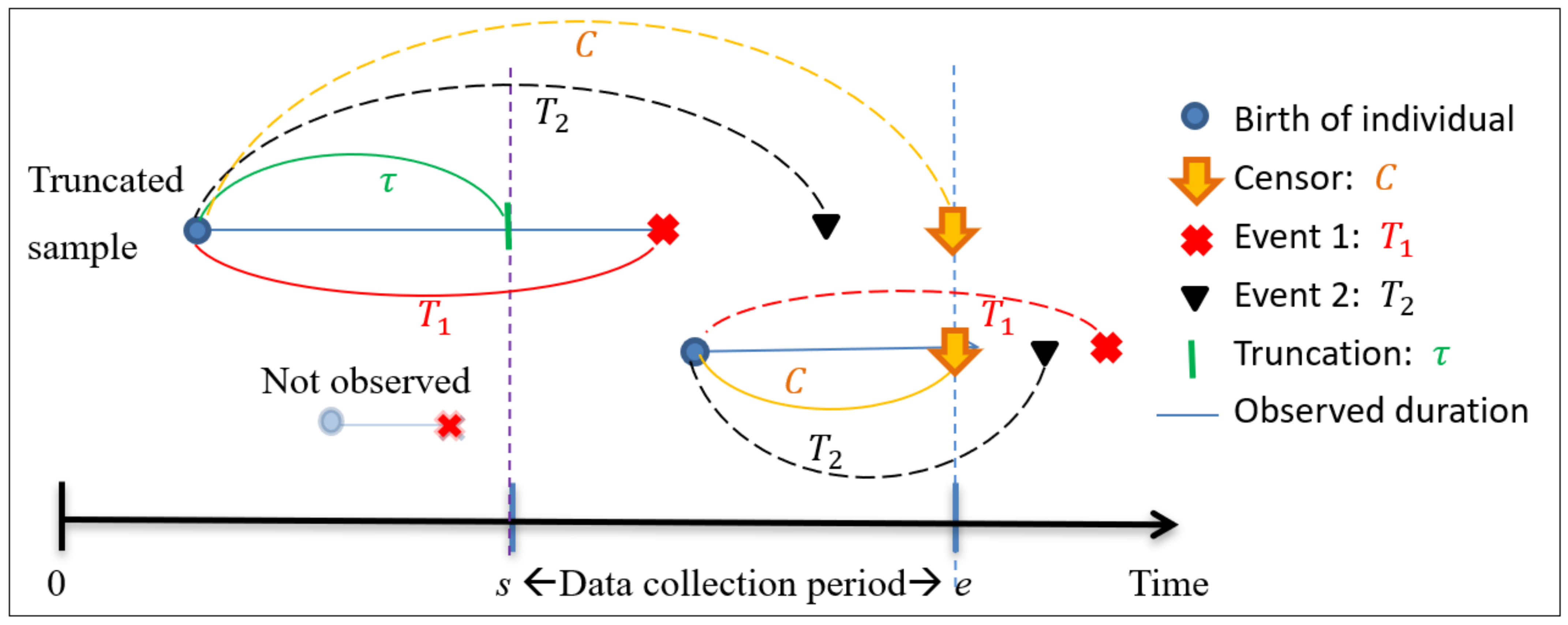
2. Left-Truncation and Competing Risks
- ,
- ,
- .
3. Proposed Methods
3.1. Copula Model for Competing Risks
3.2. Likelihood Function
- (i)
- if and ,
- (ii)
- if ,
- (iii)
- if ,
- (iv)
- if and ,
- (v)
- if ,
- (vi)
- if .
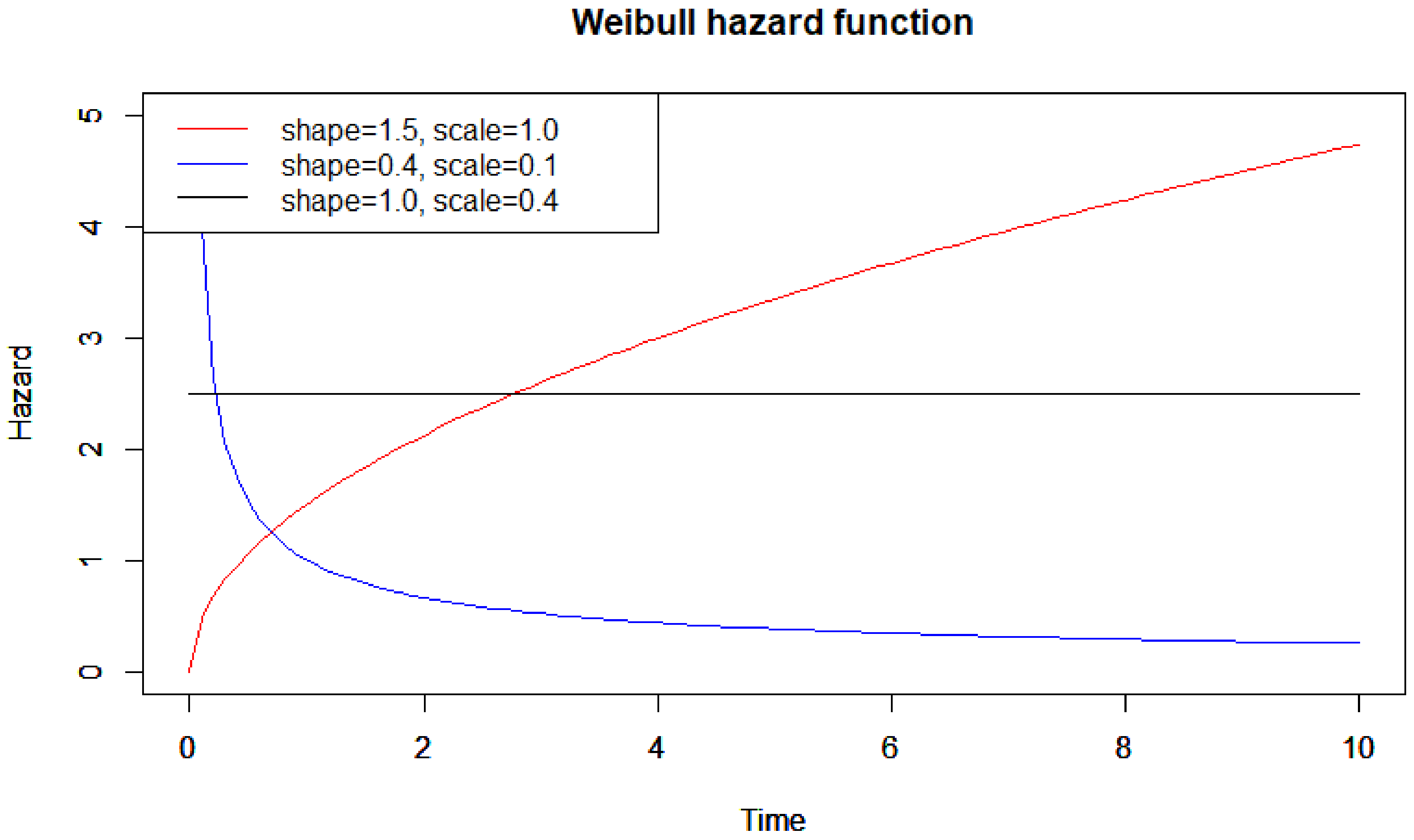
3.3. Weibull Model
4. Simulation Studies
4.1. Simulation Settings
- (a)
- Decreasing hazard: ; ; ,
- (b)
- Constant hazard: ; ; ,
- (c)
- Increasing hazard: ; ; .
4.2. Simulation Results
5. Data Analysis
6. Conclusions and Future Work
Supplementary Materials
Author Contributions
Funding
Institutional Review Board Statement
Informed Consent Statement
Data Availability Statement
Acknowledgments
Conflicts of Interest
Appendix A. Likelihood for the Gamma Model
Appendix B. Likelihood for the Lognormal Model
References
- Hong, Y.; Meeker, W.Q.; McCalley, J.D. Prediction of remaining life of power transformers based on left truncated and right censored lifetime data. Ann. Appl. Stat. 2009, 3, 857–879. [Google Scholar] [CrossRef] [Green Version]
- Emura, T.; Michimae, H. Left-truncated and right-censored field failure data: Review of parametric analysis for reliability. Qual. Reliab. Eng. Int. 2022. [Google Scholar] [CrossRef]
- Klein, J.P.; Moeschberger, M.L. Survival Analysis Techniques for Censored and Truncated Data; Springer: New York, NY, USA, 2003. [Google Scholar]
- Wang, L.; Lio, Y.; Tripathi, Y.M.; Dey, S.; Zhang, F. Inference of dependent left-truncated and right-censored competing risks data from a general bivariate class of inverse exponentiated distributions. Statistics 2022, 56, 347–374. [Google Scholar] [CrossRef]
- Lawless, J.F. Statistical Models and Methods for Lifetime Data, 2nd ed.; Wiley & Sons: Hoboken, NJ, USA, 2003. [Google Scholar]
- Li, Q.; Li, D.; Huang, B.; Jiang, Z.E.M.; Ma, J. Failure analysis for truncated and fully censored lifetime data with a hierarchical grid algorithm. IEEE Access 2020, 8, 34468–34480. [Google Scholar] [CrossRef]
- Jiang, W.; Ye, Z.; Zhao, X. Reliability estimation from left-truncated and right-censored data using splines. Stat Sin. 2020, 30, 845–875. [Google Scholar]
- Dörre, A. Semiparametric likelihood inference for heterogeneous survival data under double truncation based on a Poisson birth process. Jpn. J. Stat. Data Sci. 2021, 4, 1203–1226. [Google Scholar] [CrossRef]
- Dörre, A.; Huang, C.Y.; Tseng, Y.K.; Emura, T. Likelihood-based analysis of doubly-truncated data under the location-scale and AFT model. Comp. Stat. 2021, 36, 375–408. [Google Scholar] [CrossRef]
- Balakrishnan, N.; Mitra, D. Likelihood inference for lognormal data with left truncation and right censoring with an illustration. J. Stat. Plan Inf. 2011, 141, 3536–3553. [Google Scholar] [CrossRef]
- Balakrishnan, N.; Mitra, D. Left truncated and right censored Weibull data and likelihood inference with an illustration. Comp. Stat. Data Anal. 2012, 56, 4011–4025. [Google Scholar] [CrossRef]
- Balakrishnan, N.; Mitra, D. Some further issues concerning likelihood inference for left truncated and right censored lognormal data. Comm. Stat. Simul Comp. 2014, 43, 400–416. [Google Scholar] [CrossRef]
- Balakrishnan, N.; Mitra, D. Likelihood inference based on left truncated and right censored data from a gamma distribution. IEEE Trans. Reliab. 2013, 62, 679–688. [Google Scholar] [CrossRef]
- Balakrishnan, N.; Mitra, D. EM-based likelihood inference for some lifetime distributions based on left truncated and right censored data and associated model discrimination. S. Afr. Stat. J. 2014, 48, 125–171. [Google Scholar]
- Emura, T.; Shiu, S. Estimation and model selection for left-truncated and right-censored lifetime data with application to electric power transformers analysis. Commun. Stat. Simul. 2016, 45, 3171–3189. [Google Scholar]
- Ranjan, R.; Sen, R.; Upadhyay, S.K. Bayes analysis of some important lifetime models using MCMC based approaches when the observations are left truncated and right censored. Reliab. Eng. Syst. Saf. 2021, 214, 107747. [Google Scholar] [CrossRef]
- Mitra, D.; Kundu, D.; Balakrishnan, N. Likelihood analysis and stochastic EM algorithm for left truncated right censored data and associated model selection from the Lehmann family of life distributions. Jpn. J. Stat. Data Sci. 2021, 4, 1019–1048. [Google Scholar] [CrossRef]
- Mitra, D.; Balakrishnan, N. Statistical inference based on left truncated and interval censored data from log-location-scale family of distributions. Comm. Stat. Simul. Comp. 2021, 50, 1073–1093. [Google Scholar] [CrossRef]
- Zheng, M.; Klein, J.P. A self-consistent estimator of marginal survival functions based on dependent competing risk data and an assumed copula. Commun. Stat. Theory Methods 1994, 23, 2299–2311. [Google Scholar] [CrossRef]
- Zheng, M.; Klein, J.P. Estimates of marginal survival for dependent competing risks based on an assumed copula. Biometrika 1995, 82, 127–138. [Google Scholar] [CrossRef]
- Escarela, G.; Carriere, J.F. Fitting competing risks with an assumed copula. Stat. Methods Med. Res. 2003, 12, 333–349. [Google Scholar] [CrossRef]
- Emura, T.; Shih, J.H.; Ha, I.D.; Wilke, R.A. Comparison of the marginal hazard model and the sub-distribution hazard model for competing risks under an assumed copula. Stat. Methods Med. Res. 2020, 29, 2307–2327. [Google Scholar] [CrossRef]
- Wang, Y.C.; Emura, T.; Fan, T.H.; Lo, S.M.; Wilke, R.A. Likelihood-based inference for a frailty-copula model based on competing risks failure time data. Qual. Reliab. Eng. Int. 2020, 36, 1622–1638. [Google Scholar] [CrossRef]
- De Uña-Álvarez, J.; Veraverbeke, N. Copula-graphic estimation with left-truncated and right-censored data. Statistics 2017, 51, 387–403. [Google Scholar] [CrossRef]
- Shih, J.H.; Emura, T. Likelihood-based inference for bivariate latent failure time models with competing risks under the generalized FGM copula. Comput. Stat. 2018, 33, 1293–1323. [Google Scholar] [CrossRef]
- Kundu, D.; Mitra, D.; Ganguly, A. Analysis of left truncated and right censored competing risks data. Comp. Stat. Data Anal. 2017, 108, 12–26. [Google Scholar] [CrossRef]
- Wu, K.; Wang, L.; Yan, L.; Lio, Y. Statistical inference of left truncated and right censored data from Marshall–Olkin bivariate Rayleigh distribution. Mathematics 2021, 9, 2703. [Google Scholar] [CrossRef]
- Shuto, S.; Amemiya, T. Sequential Bayesian inference for Weibull distribution parameters with initial hyperparameter optimization for system reliability estimation. Reliab. Eng. Syst. Saf. 2022, 224, 108516. [Google Scholar] [CrossRef]
- Bouwmeester, J.; Menicucci, A.; Gill, E.K.A. Improving CubeSat reliability: Subsystem redundancy or improved testing? Reliab. Eng. Syst. Saf. 2022, 220, 108288. [Google Scholar] [CrossRef]
- Wu, C.W.; Lee, A.H.; Liu, S.W. A repetitive group sampling plan based on the lifetime performance index under gamma distribution. Qual. Reliab. Eng. Int. 2022, 38, 2049–2064. [Google Scholar] [CrossRef]
- Nelsen, R.B. An Introduction to Copulas, 2nd ed.; Springer: Berlin/Heidelberg, Germany, 2006. [Google Scholar]
- Shih, J.H.; Emura, T. Bivariate dependence measures and bivariate competing risks models under the generalized FGM copula. Stat. Pap. 2019, 60, 1101–1118. [Google Scholar] [CrossRef]
- Peng, M.; Xiang, L.; Wang, S. Semiparametric regression analysis of clustered survival data with semi-competing risks. Comp. Stat. Data Anal. 2018, 124, 53–70. [Google Scholar] [CrossRef]
- Wu, M.; Shi, Y.; Zhang, C. Statistical analysis of dependent competing risks model in accelerated life testing under progressively hybrid censoring using copula function. Commun. Stat. Simul. Comput. 2017, 46, 4004–4017. [Google Scholar] [CrossRef]
- Chesneau, C. Theoretical study of some angle parameter trigonometric copulas. Modelling 2022, 3, 140–163. [Google Scholar] [CrossRef]
- Susam, S.O. A multi-parameter Generalized Farlie-Gumbel-Morgenstern bivariate copula family via Bernstein polynomial. Hacet. J. Math. Stat. 2022, 51, 618–631. [Google Scholar] [CrossRef]
- Ota, S.; Kimura, M. Effective estimation algorithm for parameters of multivariate Farlie–Gumbel–Morgenstern copula. Jpn. J. Stat. Data Sci. 2021, 4, 1049–1078. [Google Scholar] [CrossRef]
- Ghosh, S.; Sheppard, L.W.; Holder, M.T.; Loecke, T.D.; Reid, P.C.; Bever, J.D.; Reuman, D.C. Copulas and their potential for ecology. In Advances in Ecological Research; Academic Press: Cambridge, MA, USA, 2020; Volume 62, pp. 409–468. [Google Scholar]
- Shih, J.H.; Konno, Y.; Chang, Y.T.; Emura, T. Estimation of a common mean vector in bivariate meta-analysis under the FGM copula. Statistics 2019, 53, 673–695. [Google Scholar] [CrossRef]
- Shih, J.H.; Konno, Y.; Chang, Y.T.; Emura, T. Copula-based estimation methods for a common mean vector for bivariate meta-analyses. Symmetry 2022, 14, 186. [Google Scholar] [CrossRef]
- Zhuang, H.; Diao, L.; Grace, Y.Y. A Bayesian nonparametric mixture model for grouping dependence structures and selecting copula functions. Econom. Stat. 2022, 22, 172–189. [Google Scholar] [CrossRef]
- Emura, T.; Hsu, J.H. Estimation of the Mann–Whitney effect in the two-sample problem under dependent censoring. Comp. Stat. Data Anal. 2020, 150, 106990. [Google Scholar] [CrossRef]
- Alves, M.I.F.; Neves, C. Extreme Value Distributions. Int. Encycl. Stat. Sci. 2011, 2, 493–496. [Google Scholar]
- Grimshaw, S.D. Computing maximum likelihood estimates for the generalized Pareto distribution. Technometrics 1993, 35, 185–191. [Google Scholar] [CrossRef]
- Akhter, Z.; Almetwally, E.M.; Chesneau, C. On the Generalized Bilal Distribution: Some Properties and Estimation under Ranked Set Sampling. Axioms 2022, 11, 173. [Google Scholar] [CrossRef]
- Emura, T.; Sofeu, C.L.; Rondeau, V. Conditional copula models for correlated survival endpoints: Individual patient data meta-analysis of randomized controlled trials. Stat. Method Med. Res. 2021, 30, 2634–2650. [Google Scholar] [CrossRef] [PubMed]
- Yang, Q.; He, H.; Lu, B.; Song, X. Mixture additive hazards cure model with latent variables: Application to corporate default data. Comp. Stat. Data Anal. 2022, 167, 107365. [Google Scholar] [CrossRef]
- Emura, T.; Nakatochi, M.; Matsui, S.; Michimae, H.; Rondeau, V. Personalized dynamic prediction of death according to tumour progression and high-dimensional genetic factors: Meta-analysis with a joint model. Stat. Method Med. Res. 2018, 27, 2842–2858. [Google Scholar] [CrossRef] [PubMed]
- Emura, T.; Michimae, H.; Matsui, S. Dynamic risk prediction via a joint frailty-copula model and IPD meta-analysis: Building web applications. Entropy 2022, 24, 589. [Google Scholar] [CrossRef] [PubMed]
- Kawakami, R.; Michimae, H.; Lin, Y.H. Assessing the numerical integration of dynamic prediction formulas using the exact expressions under the joint frailty-copula model. Jpn. J. Stat. Data Sci. 2021, 4, 1293–1321. [Google Scholar] [CrossRef]
- Noughabi, M.S.; Kayid, M. Bivariate quantile residual life: A characterization theorem and statistical properties. Stat. Pap. 2019, 60, 2001–2012. [Google Scholar] [CrossRef]
- Kayid, M.; Shafaei Noughabi, M.; Abouammoh, A.M. A nonparametric estimator of bivariate quantile residual life model with application to tumor recurrence data set. J. Classificat. 2020, 37, 237–253. [Google Scholar] [CrossRef]
- Zheng, R.; Najafi, S.; Zhang, Y. A recursive method for the health assessment of systems using the proportional hazards model. Reliab. Eng. Syst. Saf. 2022, 221, 108379. [Google Scholar] [CrossRef]
- Meeker, W.Q.; Hahn, G.J. A comparison of accelerated test plans to estimate the survival probability at a design stress. Technometrics 1978, 20, 245–247. [Google Scholar] [CrossRef]
- Ling, M.H. Optimal constant-stress accelerated life test plans for one-shot devices with components having exponential lifetimes under gamma frailty models. Mathematics 2022, 10, 840. [Google Scholar] [CrossRef]
- Michimae, H.; Emura, T. Bayesian ridge estimators based on copula-based joint prior distributions for regression coefficients. Comput. Stat. 2022. [Google Scholar] [CrossRef]


| True Model | Fitted Model | Event 1 | Event 2 | ||
|---|---|---|---|---|---|
| = 0.4 | = 0.1 | = 0.4 | = 0.1 | ||
| Indep. () | Indep. () | 0.406 (0.006) | 0.099 (−0.001) | 0.403 (0.003) | 0.100 (−0.000) |
| Clayton () | 0.441 (0.041) | 0.113 (0.011) | 0.437 (0.037) | 0.112 (0.012) | |
| Clayton ( MLE) | 0.457 (0.057) | 0.149 (0.049) | 0.455 (0.055) | 0.149 (0.049) | |
| Clayton ( PMLE) | 0.412 (0.012) | 0.101 (0.001) | 0.408 (0.008) | 0.101 (0.001) | |
| Clayton () | Indep. () | 0.375 (−0.025) | 0.090 (−0.010) | 0.379 (−0.021) | 0.089 (−0.011) |
| Clayton () | 0.404 (0.004) | 0.100 (−0.000) | 0.408 (0.008) | 0.100 (−0.000) | |
| Clayton ( MLE) | 0.426 (0.026) | 0.132 (0.032) | 0.428 (0.028) | 0.132 (0.032) | |
| Clayton ( PMLE) | 0.382 (−0.018) | 0.092 (−0.008) | 0.385 (−0.015) | 0.091 (−0.009) | |
| = 1.0 | = 0.4 | = 1.0 | = 0.4 | ||
| Indep. () | Indep. () | 1.003 (0.003) | 0.398 (−0.002) | 1.001 (0.001) | 0.401 (0.001) |
| Clayton () | 1.133 (0.133) | 0.557 (0.157) | 1.131 (0.131) | 0.559 (0.159) | |
| Clayton ( MLE) | 1.082 (0.082) | 0.630 (0.230) | 1.081 (0.081) | 0.631 (0.231) | |
| Clayton ( PMLE) | 1.109 (0.109) | 0.425 (0.025) | 1.107 (0.107) | 0.428 (0.028) | |
| Clayton () | Indep. () | 0.869 (−0.131) | 0.298 (−0.102) | 0.869 (−0.131) | 0.300 (−0.101) |
| Clayton () | 1.002 (0.002) | 0.399 (−0.001) | 1.001 (0.001) | 0.400 (0.000) | |
| Clayton ( MLE) | 0.952 (−0.048) | 0.470 (0.070) | 0.951 (−0.049) | 0.471 (0.071) | |
| Clayton ( PMLE) | 0.934 (−0.066) | 0.313 (−0.087) | 0.934 (−0.066) | 0.314 (−0.086) | |
| = 1.5 | = 1.0 | = 1.5 | = 1.0 | ||
| Indep. () | Indep. () | 1.500 (−0.000) | 1.002 (0.002) | 1.501 (0.001) | 1.001 (0.001) |
| Clayton () | 1.684 (0.184) | 1.575 (0.575) | 1.685 (0.185) | 1.574 (0.574) | |
| Clayton ( MLE) | 1.642 (0.142) | 1.225 (0.225) | 1.643 (0.143) | 1.223 (0.223) | |
| Clayton ( PMLE) | 1.671 (0.171) | 1.193 (0.193) | 1.672 (0.172) | 1.191 (0.191) | |
| Clayton () | Indep. () | 1.315 (−0.185) | 0.666 (−0.334) | 1.316 (−0.184) | 0.665 (−0.335) |
| Clayton () | 1.502 (0.001) | 1.002 (0.002) | 1.503 (0.003) | 1.002 (0.002) | |
| Clayton ( MLE) | 1.496 (−0.004) | 0.991 (−0.009) | 1.496 (−0.004) | 0.990 (−0.010) | |
| Clayton ( PMLE) | 1.426 (−0.073) | 0.747 (−0.025) | 1.426 (−0.073) | 0.746 (−0.253) | |
| True Model | Fitted Model | Event 1 | Event 2 | ||
|---|---|---|---|---|---|
| = 0.4 | = 0.1 | = 0.4 | = 0.1 | ||
| 0.00186 | 0.00017 | 0.00170 | 0.00017 | ||
| 0.00374 | 0.00035 | 0.00335 | 0.00036 | ||
| Clayton ( MLE) | 0.00517 | 0.00320 | 0.00498 | 0.00321 | |
| Clayton ( PMLE) | 0.00204 | 0.00018 | 0.00184 | 0.00017 | |
| 0.00229 | 0.00025 | 0.00221 | 0.00028 | ||
| 0.00195 | 0.00018 | 0.00207 | 0.00020 | ||
| Clayton ( MLE) | 0.00261 | 0.00178 | 0.00274 | 0.00178 | |
| Clayton ( PMLE) | 0.00210 | 0.00022 | 0.00204 | 0.00025 | |
| = 1.0 | = 0.4 | = 1.0 | = 0.4 | ||
| 0.00111 | 0.00093 | 0.00111 | 0.00087 | ||
| 0.01847 | 0.02621 | 0.01799 | 0.02673 | ||
| Clayton ( MLE) | 0.00115 | 0.07285 | 0.01124 | 0.07301 | |
| Clayton ( PMLE) | 0.01323 | 0.00175 | 0.01266 | 0.00184 | |
| 0.01831 | 0.01095 | 0.01814 | 0.01066 | ||
| 0.00102 | 0.00090 | 0.00088 | 0.00081 | ||
| Clayton ( MLE) | 0.00629 | 0.01394 | 0.00622 | 0.01385 | |
| Clayton ( PMLE) | 0.00575 | 0.00828 | 0.00560 | 0.00803 | |
| = 1.5 | = 1.0 | = 1.5 | = 1.0 | ||
| 0.00229 | 0.00346 | 0.00244 | 0.00314 | ||
| 0.03547 | 0.33575 | 0.03570 | 0.33428 | ||
| Clayton ( MLE) | 0.02966 | 0.08040 | 0.02991 | 0.08363 | |
| Clayton ( PMLE) | 0.03181 | 0.04223 | 0.03254 | 0.04108 | |
| 0.03659 | 0.11357 | 0.03642 | 0.11415 | ||
| 0.00193 | 0.00300 | 0.00179 | 0.00297 | ||
| Clayton ( MLE) | 0.00294 | 0.00875 | 0.00282 | 0.00867 | |
| Clayton ( PMLE) | 0.00830 | 0.00664 | 0.00808 | 0.06680 | |
| True Par. | True Model | Fitted Model | ||||
|---|---|---|---|---|---|---|
| Indep. () | Indep. () | 0.00369 | 0.00186 | 0.00114 | 0.00096 | |
| Clayton () | 0.00614 | 0.00374 | 0.00261 | 0.00240 | ||
| Clayton ( MLE) | 0.00706 | 0.00517 | 0.00404 | 0.00417 | ||
| Clayton ( PMLE) | 0.00412 | 0.00204 | 0.00122 | 0.00104 | ||
| Clayton () | Indep. () | 0.00394 | 0.00229 | 0.00174 | 0.00145 | |
| Clayton () | 0.00404 | 0.00195 | 0.00134 | 0.00094 | ||
| Clayton ( MLE) | 0.00408 | 0.00261 | 0.00215 | 0.00180 | ||
| Clayton ( PMLE) | 0.00382 | 0.00209 | 0.00153 | 0.00122 | ||
| Indep. () | Indep. () | 0.00239 | 0.00111 | 0.00073 | 0.00053 | |
| Clayton () | 0.01950 | 0.01847 | 0.01738 | 0.01743 | ||
| Clayton ( MLE) | 0.01295 | 0.00115 | 0.00955 | 0.00927 | ||
| Clayton ( PMLE) | 0.00147 | 0.01323 | 0.01204 | 0.01179 | ||
| Clayton () | Indep. () | 0.01967 | 0.01831 | 0.01818 | 0.01800 | |
| Clayton () | 0.00195 | 0.00102 | 0.00065 | 0.00047 | ||
| Clayton ( MLE) | 0.00678 | 0.00629 | 0.00728 | 0.00720 | ||
| Clayton ( PMLE) | 0.00717 | 0.00575 | 0.00543 | 0.00523 | ||
| Indep. () | Indep. () | 0.00457 | 0.00229 | 0.00161 | 0.00110 | |
| Clayton () | 0.03838 | 0.03547 | 0.03474 | 0.03482 | ||
| Clayton ( MLE) | 0.03402 | 0.02966 | 0.02840 | 0.02907 | ||
| Clayton ( PMLE) | 0.03612 | 0.03181 | 0.03141 | 0.03109 | ||
| Clayton () | Indep. () | 0.03807 | 0.03659 | 0.03572 | 0.03527 | |
| Clayton () | 0.00394 | 0.00193 | 0.00127 | 0.00091 | ||
| Clayton ( MLE) | 0.00605 | 0.00294 | 0.00179 | 0.00129 | ||
| Clayton ( PMLE) | 0.01083 | 0.008300. | 0.00729 | 0.00676 |
| True Model | Fitted Model | = 0.4 | = 0.1 | = 0.4 | = 0.1 | ||||
|---|---|---|---|---|---|---|---|---|---|
| SD | SE | SD | SE | SD | SE | SD | SE | ||
| 0.043 | 0.042 | 0.013 | 0.013 | 0.041 | 0.042 | 0.013 | 0.013 | ||
| 0.046 | 0.044 | 0.015 | 0.014 | 0.044 | 0.044 | 0.014 | 0.014 | ||
| Clayton ( PMLE) | 0.044 | 0.043 | 0.013 | 0.013 | 0.042 | 0.042 | 0.013 | 0.013 | |
| 0.041 | 0.043 | 0.012 | 0.012 | 0.042 | 0.043 | 0.013 | 0.012 | ||
| 0.044 | 0.044 | 0.013 | 0.014 | 0.045 | 0.044 | 0.014 | 0.014 | ||
| Clayton ( PMLE) | 0.042 | 0.043 | 0.012 | 0.013 | 0.043 | 0.043 | 0.013 | 0.013 | |
| = 1.0 | = 0.4 | = 1.0 | = 0.4 | ||||||
| SD | SE | SD | SE | SD | SE | SD | SE | ||
| 0.033 | 0.033 | 0.030 | 0.029 | 0.033 | 0.033 | 0.029 | 0.029 | ||
| 0.029 | 0.028 | 0.038 | 0.035 | 0.028 | 0.028 | 0.036 | 0.035 | ||
| Clayton ( PMLE) | 0.036 | 0.034 | 0.034 | 0.031 | 0.036 | 0.034 | 0.033 | 0.031 | |
| 0.035 | 0.035 | 0.024 | 0.024 | 0.033 | 0.035 | 0.024 | 0.024 | ||
| 0.032 | 0.031 | 0.030 | 0.029 | 0.030 | 0.031 | 0.029 | 0.029 | ||
| Clayton ( PMLE) | 0.037 | 0.036 | 0.026 | 0.025 | 0.035 | 0.036 | 0.025 | 0.025 | |
| = 1.5 | = 1.0 | = 1.5 | = 1.0 | ||||||
| SD | SE | SD | SE | SD | SE | SD | SE | ||
| 0.048 | 0.049 | 0.059 | 0.058 | 0.049 | 0.049 | 0.056 | 0.058 | ||
| 0.040 | 0.040 | 0.075 | 0.076 | 0.040 | 0.040 | 0.073 | 0.076 | ||
| Clayton ( PMLE) | 0.051 | 0.050 | 0.071 | 0.067 | 0.053 | 0.050 | 0.068 | 0.067 | |
| 0.049 | 0.050 | 0.043 | 0.043 | 0.049 | 0.050 | 0.042 | 0.043 | ||
| 0.044 | 0.043 | 0.055 | 0.055 | 0.042 | 0.043 | 0.055 | 0.055 | ||
| Clayton ( PMLE) | 0.054 | 0.051 | 0.050 | 0.048 | 0.052 | 0.051 | 0.049 | 0.048 | |
(Index) | (Install) | (End) | (Truncation) | Event | (Truncation Time) | (Failure Time) |
|---|---|---|---|---|---|---|
| 1 | 1961 | 1996 | 0 | 2 | 19 | 35 |
| 2 | 1964 | 1985 | 0 | 1 | 16 | 21 |
| 3 | 1962 | 2007 | 0 | 2 | 18 | 45 |
| 4 | 1962 | 1986 | 0 | 2 | 18 | 24 |
| 5 | 1961 | 1992 | 0 | 2 | 19 | 31 |
| : | : | : | : | : | : | : |
| 30 | 1963 | 1994 | 0 | 1 | 17 | 31 |
| 31 | 1987 | 2008 | 1 | 0 | Undefined | 21 |
| 32 | 1980 | 2008 | 1 | 0 | Undefined | 28 |
| 33 | 1988 | 2008 | 1 | 0 | Undefined | 20 |
| 34 | 1985 | 2008 | 1 | 0 | Undefined | 23 |
| : | : | : | : | : | : | : |
| 100 | 1989 | 2008 | 1 | 0 | Undefined | 19 |
| ; Shape | ; Scale | ; Shape | ; Scale | logL | ||
|---|---|---|---|---|---|---|
| * | - | 2.82 (0.61) | 6.93 (5.24) | 2.79 (0.39) | 15.77 (7.73) | −8.984 |
| - | 3.18 (0.65) | 12.86 (10.56) | 2.88 (0.40) | 18.74 (9.29) | −9.024 | |
| - | 3.68 (0.57) | 33.12 (22.90) | 2.93 (0.38) | 21.93 (10.19) | −9.389 | |
| - | 3.39 (0.40) | 35.97 (16.21) | 2.92 (0.35) | 24.65 (10.64) | −9.239 | |
| MLE | 0.004 (0.11) | 2.82 (0.60) | 6.96 (5.16) | 2.79 (0.39) | 15.79 (7.70) | −8.983 |
| PMLE () | 0.402 | 3.12 (0.65) | 11.57 (9.42) | 2.87 (0.40) | 18.31 (9.10) | −9.008 |
| PMLE () | 1.853 | 3.66 (0.59) | 31.57 (22.44) | 2.93 (0.38) | 21.73 (10.15) | −9.384 |
| PMLE () | 8.179 | 3.38 (0.40) | 35.77 (16.07) | 2.92 (0.35) | 24.67 (10.63) | −9.238 |
| Results of [26] | - | 2.80 (-) | 6.76 (-) | 2.80 (-) | 15.93 (-) | - |
Publisher’s Note: MDPI stays neutral with regard to jurisdictional claims in published maps and institutional affiliations. |
© 2022 by the authors. Licensee MDPI, Basel, Switzerland. This article is an open access article distributed under the terms and conditions of the Creative Commons Attribution (CC BY) license (https://creativecommons.org/licenses/by/4.0/).
Share and Cite
Michimae, H.; Emura, T. Likelihood Inference for Copula Models Based on Left-Truncated and Competing Risks Data from Field Studies. Mathematics 2022, 10, 2163. https://doi.org/10.3390/math10132163
Michimae H, Emura T. Likelihood Inference for Copula Models Based on Left-Truncated and Competing Risks Data from Field Studies. Mathematics. 2022; 10(13):2163. https://doi.org/10.3390/math10132163
Chicago/Turabian StyleMichimae, Hirofumi, and Takeshi Emura. 2022. "Likelihood Inference for Copula Models Based on Left-Truncated and Competing Risks Data from Field Studies" Mathematics 10, no. 13: 2163. https://doi.org/10.3390/math10132163