
An Improved Arithmetic Optimization Algorithm for Numerical Optimization Problems


Abstract
:1. Introduction
2. Preliminaries
2.1. Nonlinear Equation Systems
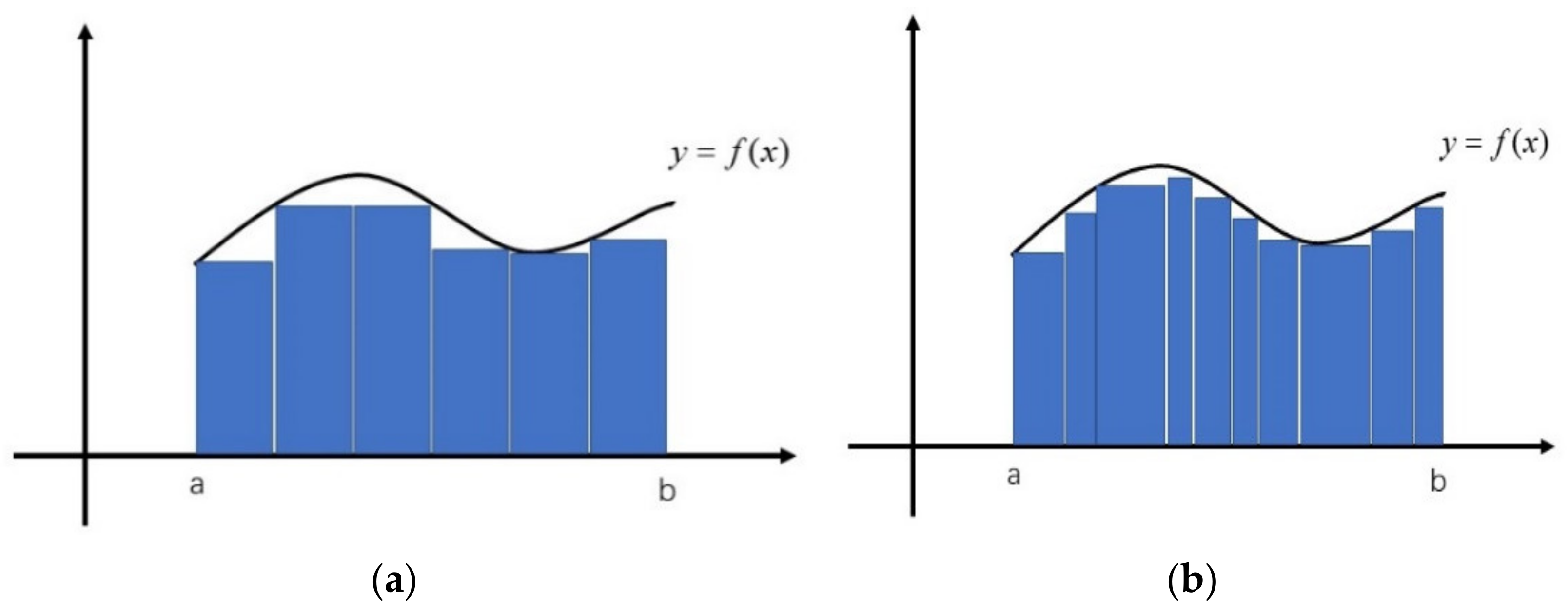
2.2. Numerical Integration
- (1)
- Randomly initialize the population in the search space S.
- (2)
- Arrange each individual in the integral interval in ascending order. The integral interval has n(n = D + 2) nodes and n − 1 segments. Calculate the distance hi between two adjacent nodes and the function f(xk) value of each node, then calculate the function value corresponding to the D + 2 nodes and the function value of the middle node of each subsection. Find the minimum value wj and the maximum value Wj (j = 1, 2, …, D + 1) among the function values of the left endpoint, middle node, and right endpoint of each subsection.
- (3)
- Calculate fitness value. .
- (4)
- Update individuals through an optimization algorithm.
- (5)
- Repeat step 4 until reaching the stop condition.
- (6)
- Get the accuracy and integral values.
- (1)
- Randomly initialize the population in the search space S.
- (2)
- Arrange each individual in the integral interval in ascending order. The integral interval has n(n = D + 2) nodes and n − 1 segments. Calculate the distance hi between two adjacent nodes and the function f(xk) value of each node and then bring them into Equation (5).
- (3)
- Calculate the fitness value by Equation (6).
- (4)
- Update individuals through an optimization algorithm.
- (5)
- Repeat step 4 until reaching the stop condition.
- (6)
- Get the accuracy and integral values.
2.3. The Arithmetic Optimization Algorithm (AOA)
2.3.1. Initialization Phase
2.3.2. Exploration Phase
2.3.3. Exploitation Phase
| Algorithm 1 AOA |
| 1. Set up the initial parameters α, μ. 2. Initialize the population randomly. 3. for t = 1: T 4. Calculate the fitness function and select the best solution. 5. Update the MOA (using Equation (8)) and MOP (using Equation (10)). 6. for i = 1: N 7. for j = 1: Dim 8. Generate the random values between [0, 1] (r1, r2, r3) 9. if r1 > MOA 10. if r2 > 0.5 11. Update the position of the individual by Equation (9). 12. else 13. Update the position of the individual by Equation (9). 14. end 15. else 16. if r3 > 0.5 17. Update the position of the individual by Equation (11). 18. else 19. Update the position of the individual by Equation (11). 20. end 21. end 22. end 23. end 24. t = t + 1 25. end 26. Return the best solution (x). |
3. Our Proposed IAOA
3.1. Motivation for Improving the AOA
3.2. Population Control Mechanism
3.2.1. The First Subpopulation
3.2.2. The Second Subpopulation
3.2.3. The Third Subpopulation
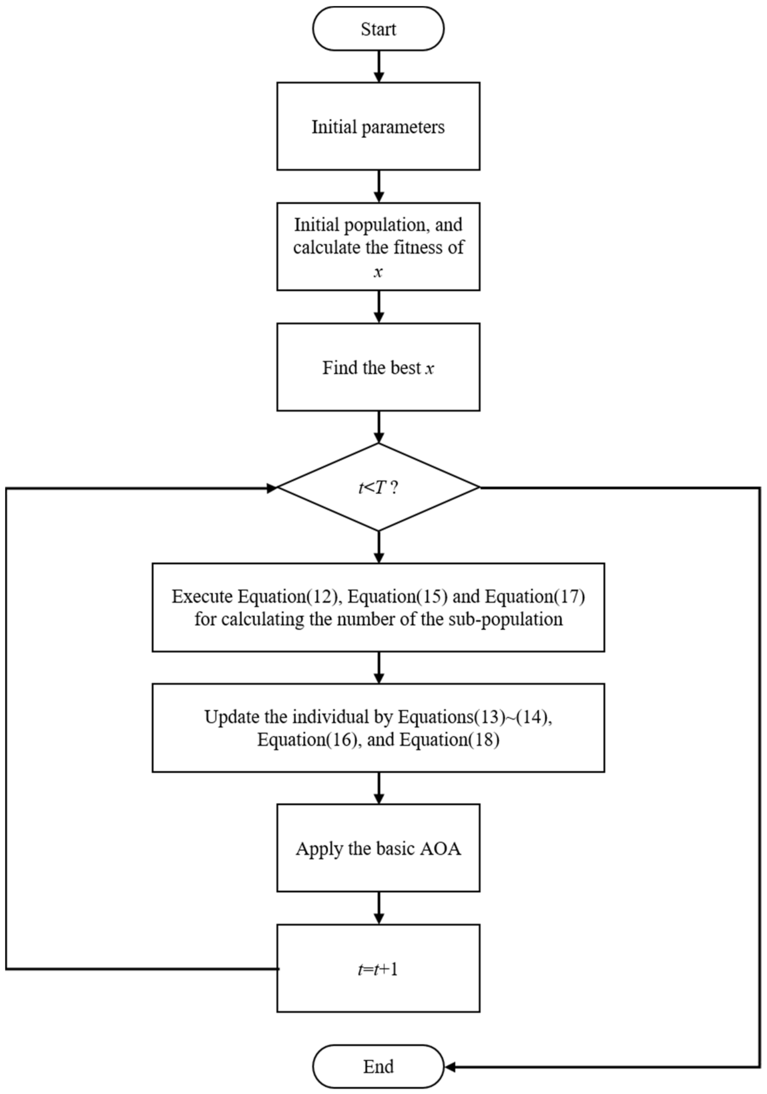
| Algorithm 2 IAOA |
| 1. Set up the initial parameters α, μ. 2. Initialize the population randomly. 3. for t = 1: T 4. Calculate the fitness function and select the best solution. 5. Calculate the number of the first subpopulation by Equation (12). 6. Update the first subpopulation by Equations (13) and (14). 7. Calculate the number of the second subpopulation by Equation (15). 8. Update the second subpopulation by Equation (16). 9. Calculate the number of the third subpopulation by Equation (17). 10. Update the third subpopulation by Equation (18). 11. Update the MOA (using Equation (8)) and MOP (using Equation (10)). 12. for i = 1: N 13. for j = 1: Dim 14. Generate the random values between [0, 1] (r1, r2, r3) 15. if r1 > MOA 16. if r2 > 0.5 17. Update the position of the individual by Equation (9). 18. else 19. Update the position of the individual by Equation (9). 20. end 21. else 22. if r3 > 0.5 23. Update the position of the individual by Equation (11). 24. else 25. Update the position of the individual by Equation (11). 26. end 27. end 28. end 29. end 30. t = t + 1 31. end 32. Return the best solution (x). |
4. Numerical Experiments and Analysis
4.1. Parameter Settings
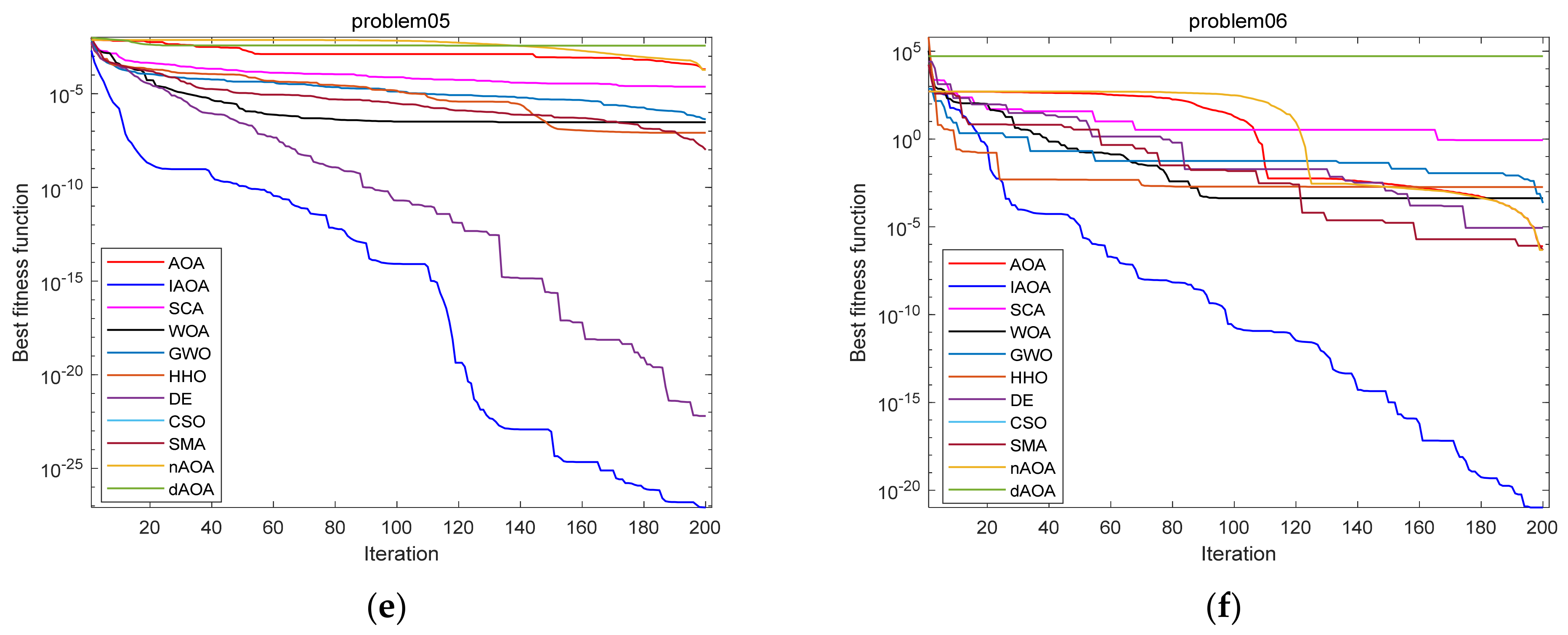
4.2. Application in Solving NESs
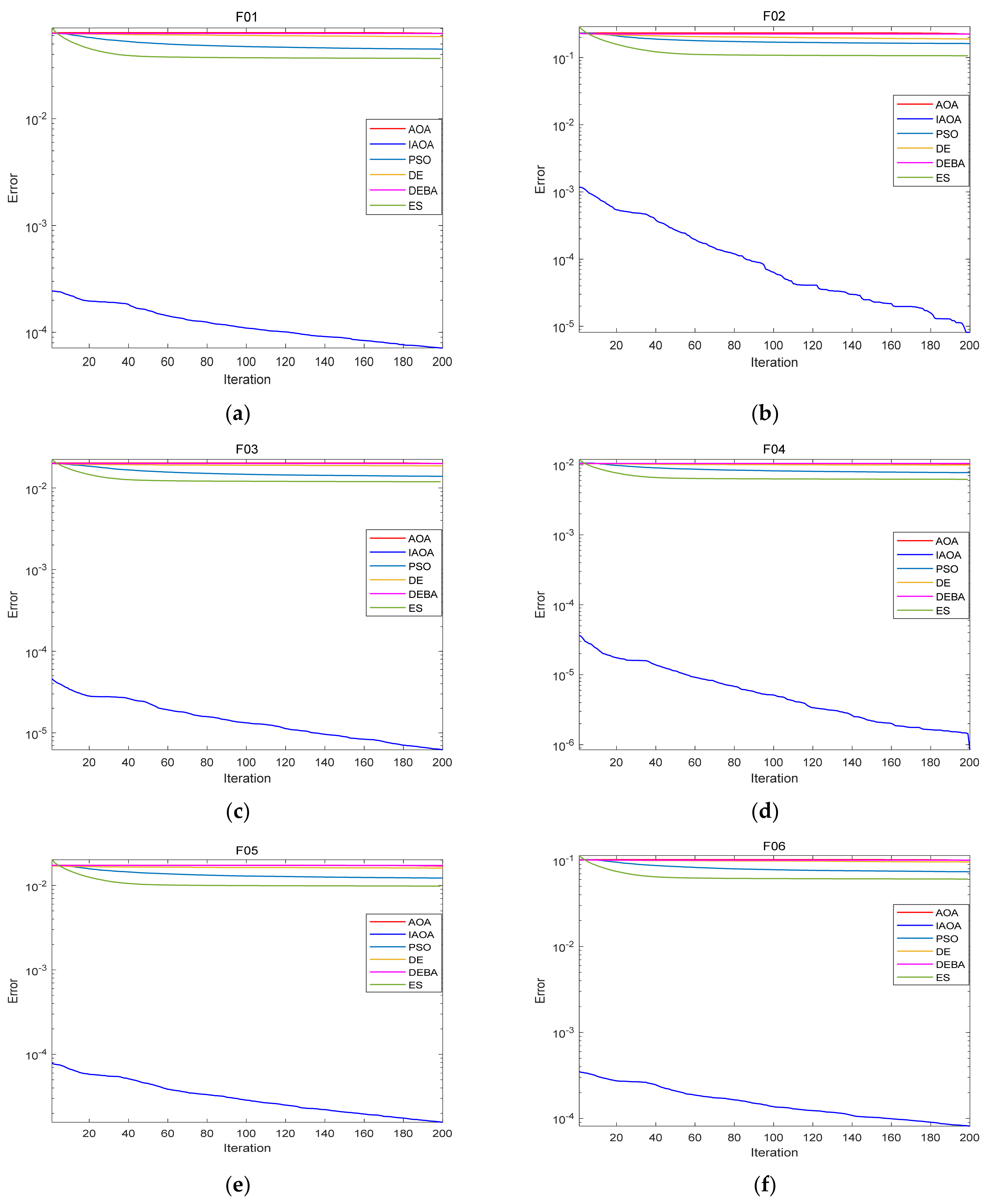
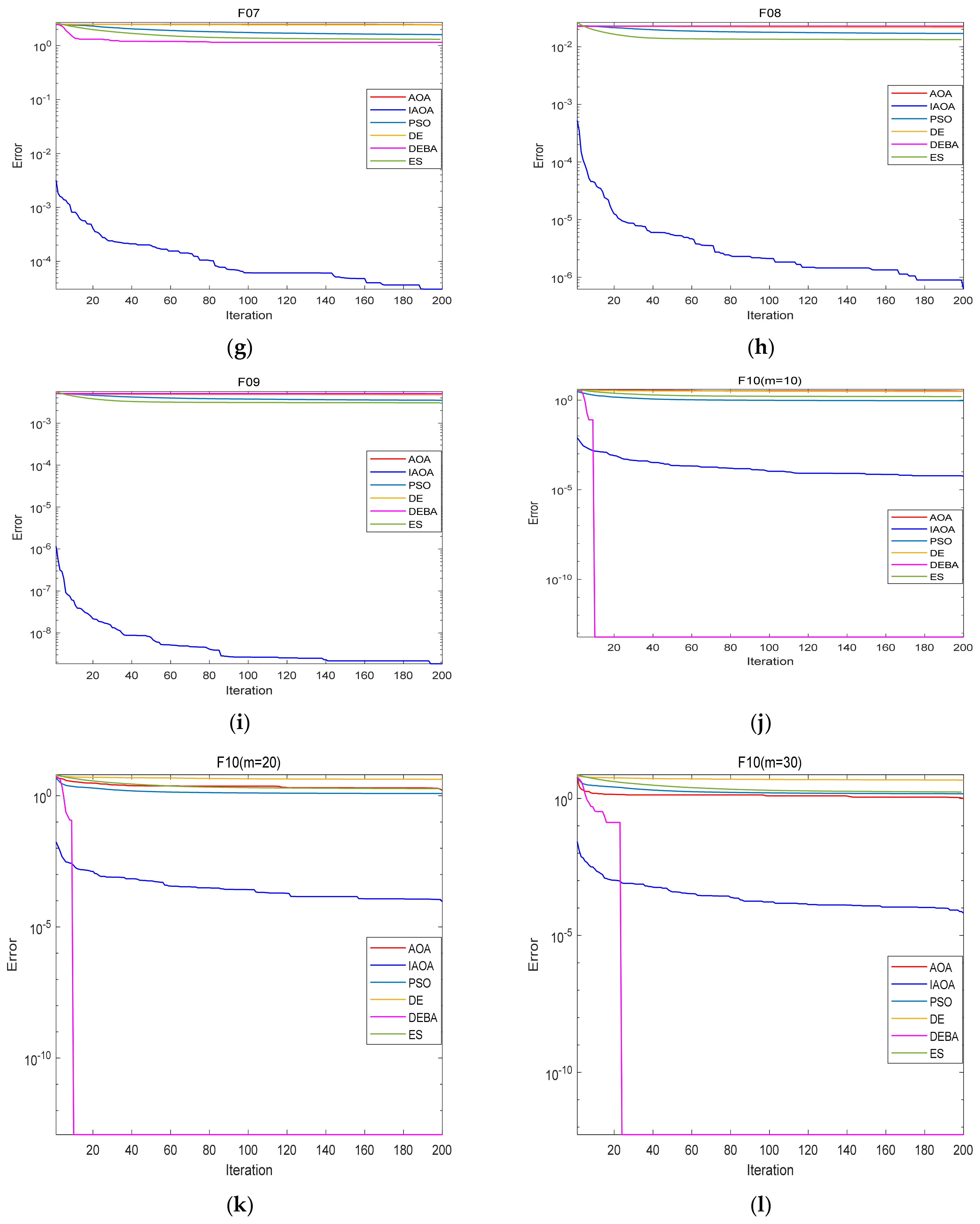
4.3. Numerical Integration
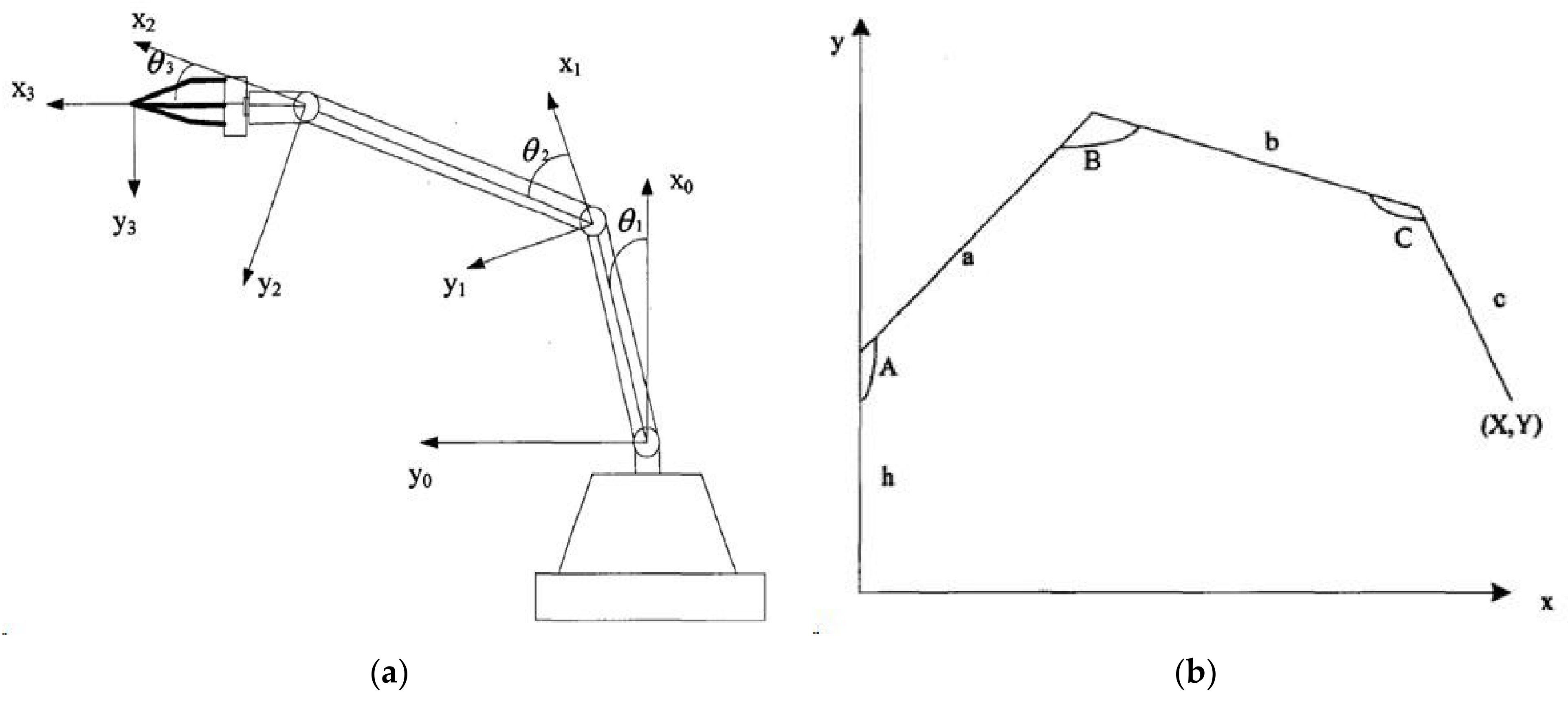
4.4. Sovling Engineering Problem
5. Conclusions and Future Works
Author Contributions
Funding
Institutional Review Board Statement
Informed Consent Statement
Data Availability Statement
Conflicts of Interest
References
- Broyden, C.G. A class of methods for solving nonlinear simultaneous equations. Math. Comput. 1965, 19, 577–593. [Google Scholar] [CrossRef]
- Ramos, H.; Monteiro, M.T.T. A new approach based on the newton’s method to solve systems of nonlinear equations. J. Comput. Appl. Math. 2017, 318, 3–13. [Google Scholar] [CrossRef]
- Hueso, J.L.; Martínez, E.; Torregrosa, J.R. Modified newton’s method for systems of nonlinear equations with singular Jacobian. J. Comput. Appl. Math. 2009, 224, 77–83. [Google Scholar] [CrossRef] [Green Version]
- Luo, Y.Z.; Tang, G.J.; Zhou, L.N. Hybrid approach for solving systems of nonlinear equations using chaos optimization and quasi-newton method. Appl. Soft Comput. 2008, 8, 1068–1073. [Google Scholar] [CrossRef]
- Karr, C.L.; Weck, B.; Freeman, L.M. Solutions to systems of nonlinear equations via a genetic algorithm. Eng. Appl. Artif. Intell. 1998, 11, 369–375. [Google Scholar] [CrossRef]
- Ouyang, A.J.; Zhou, Y.Q.; Luo, Q.F. Hybrid particle swarm optimization algorithm for solving systems of nonlinear equations. In Proceedings of the 2009 IEEE International Conference on Granular Computing, Nanchang, China, 17–19 August 2009; pp. 460–465. [Google Scholar]
- Jaberipour, M.; Khorram, E.; Karimi, B. Particle swarm algorithm for solving systems of nonlinear equations. Comput. Math. Appl. 2011, 62, 566–576. [Google Scholar] [CrossRef] [Green Version]
- Pourjafari, E.; Mojallali, H. Solving nonlinear equations systems with a new approach based on invasive weed optimization algorithm and clustering. Swarm Evol. Comput. 2012, 4, 33–43. [Google Scholar] [CrossRef]
- Jia, R.M.; He, D.X. Hybrid artificial bee colony algorithm for solving nonlinear system of equations. In Proceedings of the 2012 Eighth International Conference on Computational Intelligence and Security, Guangzhou, China, 17–18 November 2012; pp. 56–60. [Google Scholar]
- Ren, H.M.; Wu, L.; Bi, W.H.; Argyros, I.K. Solving nonlinear equations system via an efficient genetic algorithm with symmetric and harmonious individuals. Appl. Math. Comput. 2013, 219, 10967–10973. [Google Scholar] [CrossRef]
- Cai, R.Z.; Yue, G.L. A novel firefly algorithm of solving nonlinear equation group. Appl. Mech. Mater. 2013, 389, 918–923. [Google Scholar]
- Abdollahi, M.; Isazadeh, A.; Abdollahi, D. Imperialist competitive algorithm for solving systems of nonlinear equations. Comput. Math. Appl. 2013, 65, 1894–1908. [Google Scholar] [CrossRef]
- Hirsch, M.J.; Pardalos, P.M.; Resende, M.G.C. Solving systems of nonlinear equations with continuous GRASP. Nonlinear Anal. Real World Appl. 2009, 10, 2000–2006. [Google Scholar] [CrossRef]
- Sacco, W.F.; Henderson, N. Finding all solutions of nonlinear systems using a hybrid metaheuristic with fuzzy clustering means. Appl. Soft Comput. 2011, 11, 5424–5432. [Google Scholar] [CrossRef]
- Gong, W.Y.; Wang, Y.; Cai, Z.H.; Yang, S. A weighted bi-objective transformation technique for locating multiple optimal solutions of nonlinear equation systems. IEEE Trans. Evol. Comput. 2017, 21, 697–713. [Google Scholar] [CrossRef] [Green Version]
- Ariyaratne, M.K.A.; Fernando, T.G.I.; Weerakoon, S. Solving systems of nonlinear equations using a modified firefly algorithm (MODFA). Swarm Evol. Comput. 2019, 48, 72–92. [Google Scholar] [CrossRef]
- Gong, W.Y.; Wang, Y.; Cai, Z.H.; Wang, L. Finding multiple roots of nonlinear equation systems via a repulsion-based adaptive differential evolution. IEEE Trans. Syst. Man Cybern. Syst. 2020, 50, 1499–1513. [Google Scholar] [CrossRef] [Green Version]
- Ibrahim, A.M.; Tawhid, M.A. A hybridization of differential evolution and monarch butterfly optimization for solving systems of nonlinear equations. J. Comput. Des. Eng. 2019, 6, 354–367. [Google Scholar] [CrossRef]
- Liao, Z.W.; Gong, W.Y.; Wang, L. Memetic niching-based evolutionary algorithms for solving nonlinear equation system. Expert Syst. Appl. 2020, 149, 113–261. [Google Scholar] [CrossRef]
- Ning, G.Y.; Zhou, Y.Q. Application of improved differential evolution algorithm in solving equations. Int. J. Comput. Intell. Syst. 2021, 14, 199. [Google Scholar] [CrossRef]
- Rizk-Allah, R.M. A quantum-based sine cosine algorithm for solving general systems of nonlinear equations. Artif. Intell. Rev. 2021, 54, 3939–3990. [Google Scholar] [CrossRef]
- Ji, J.Y.; Man, L.W. An improved dynamic multi-objective optimization approach for nonlinear equation systems. Inf. Sci. 2021, 576, 204–227. [Google Scholar] [CrossRef]
- Turgut, O.E.; Turgut, M.S.; Coban, M.T. Chaotic quantum behaved particle swarm optimization algorithm for solving nonlinear system of equations. Comput. Math. Appl. 2014, 68, 508–530. [Google Scholar] [CrossRef]
- Zhou, Y.Q.; Zhang, M.; Zhao, B. Numerical integration of arbitrary functions based on evolutionary strategy method. Chin. J. Comput. 2008, 21, 196–206. [Google Scholar]
- Wei, X.Q.; Zhou, Y.Q. Research on numerical integration method based on particle swarm optimization. Microelectron. Comput. 2009, 26, 117–119. [Google Scholar]
- Wei, X.X.; Zhou, Y.Q.; Lan, X.L. Research on a numerical integration method based on functional networks. Comput. Sci. 2009, 36, 224–226. [Google Scholar]
- Deng, Z.X.; Huang, F.D.; Liu, X.J. A differential evolution algorithm for solving numerical integration problems. Comput. Eng. 2011, 37, 206–207. [Google Scholar]
- Xiao, H.H.; Duan, Y.M. Application of improved bat algorithm in numerical integration. J. Intell. Syst. 2014, 9, 364–371. [Google Scholar]
- Szczepanski, R.; Kaminski, M.; Tarczewski, T. Auto-tuning process of state feedback speed controller applied for two-mass system. Energies 2020, 13, 3067. [Google Scholar] [CrossRef]
- Hu, H.B.; Hu, Q.B.; Lu, Z.Y.; Xu, D. Optimal PID controller design in PMSM servo system via particle swarm optimization. In Proceedings of the 31st Annual Conference of IEEE Industrial Electronics Society, IECON 2005, Raleigh, NC, USA, 6–10 November 2005; p. 5. [Google Scholar]
- Szczepanski, R.; Tarczewski, T.; Niewiara, L.J.; Stojic, D. Isdentification of mechanical parameters in servo-drive system. In Proceedings of the 2021 IEEE 19th International Power Electronics and Motion Control Conference (PEMC), Gliwice, Poland, 25–29 April 2021; pp. 566–573. [Google Scholar]
- Liu, L.; Cartes, D.A.; Liu, W. Particle Swarm Optimization Based Parameter Identification Applied to PMSM. In Proceedings of the 2007 American Control Conference, New York, NY, USA, 9–13 July 2007; pp. 2955–2960. [Google Scholar]
- Szczepanski, R.; Tarczewski, T. Global path planning for mobile robot based on artificial bee colony and Dijkstra’s algorithms. In Proceedings of the 2021 IEEE 19th International Power Electronics and Motion Control Conference (PEMC), Gliwice, Poland, 25–29 April 2021; pp. 724–730. [Google Scholar]
- Brand, M.; Masuda, M.; Wehner, N.; Yu, X.H. Ant colony optimization algorithm for robot path planning. In Proceedings of the 2010 International Conference on Computer Design and Applications, Qinhuangdao, China, 25–27 June 2010; pp. 436–440. [Google Scholar]
- Szczepanski, R.; Erwinski, K.; Tejer, M.; Bereit, A.; Tarczewski, T. Optimal scheduling for palletizing task using robotic arm and artificial bee colony algorithm. Eng. Appl. Artif. Intell. 2022, 113, 104976. [Google Scholar] [CrossRef]
- Kolakowska, E.; Smith, S.F.; Kristiansen, M. Constraint optimization model of a scheduling problem for a robotic arm in automatic systems. Robot. Auton. Syst. 2014, 62, 267–280. [Google Scholar] [CrossRef]
- Abualigah, L.; Diabat, A.; Mirjalili, S.; Abd Elaziz, M.; Gandomi, A.H. The arithmetic optimization algorithm. Comput. Methods Appl. Mech. Eng. 2021, 376, 113609. [Google Scholar] [CrossRef]
- Premkumar, M.; Jangir, P.; Kumar, D.S.; Sowmya, R.; Alhelou, H.H.; Abualigah, L.; Yildiz, A.R.; Mirjalili, S. A new arithmetic optimization algorithm for solving real-world multi-objective CEC-2021 constrained optimization problems: Diversity analysis and validations. IEEE Access 2021, 9, 84263–84295. [Google Scholar] [CrossRef]
- Bansal, P.; Gehlot, K.; Singhal, A.; Gupta, A. Automatic detection of osteosarcoma based on integrated features and feature selection using binary arithmetic optimization algorithm. Multimed. Tools Appl. 2022, 81, 8807–8834. [Google Scholar] [CrossRef]
- Agushaka, J.O.; Ezugwu, A.E. Advanced arithmetic optimization algorithm for solving mechanical engineering design problems. PLoS ONE 2021, 16, e0255703. [Google Scholar]
- Abualigah, L.; Diabat, A.; Sumari, P.; Gandomi, A. A novel evolutionary arithmetic optimization algorithm for multilevel thresholding segmentation of COVID-19 CT images. Processes 2021, 9, 1155. [Google Scholar] [CrossRef]
- Xu, Y.P.; Tan, J.W.; Zhu, D.J.; Ouyang, P.; Taheri, B. Model identification of the proton exchange membrane fuel cells by extreme learning machine and a developed version of arithmetic optimization algorithm. Energy Rep. 2021, 7, 2332–2342. [Google Scholar] [CrossRef]
- Izci, D.; Ekinci, S.; Kayri, M.; Eker, E. A novel improved arithmetic optimization algorithm for optimal design of PID controlled and Bode’s ideal transfer function-based automobile cruise control system. Evol. Syst. 2021, 13, 453–468. [Google Scholar] [CrossRef]
- Khatir, S.; Tiachacht, S.; Thanh, C.L.; Ghandourah, E.; Mirjalili, S.; Wahab, M.A. An improved artificial neural network using arithmetic optimization algorithm for damage assessment in FGM composite plates. Compos. Struct. 2021, 273, 114–287. [Google Scholar] [CrossRef]
- Viswanathan, G.M.; Afanasyev, V.; Buldyrev, S.; Murphy, E.J.; Prince, P.A.; Stanley, H.E. Lévy flight search patterns of wandering albatrosses. Nature 1996, 381, 413–415. [Google Scholar] [CrossRef]
- Humphries, N.E.; Queiroz, N.; Dyer, J.R.; Pade, N.G.; Musyl, M.K.; Schaefer, K.M.; Fuller, D.W.; Brunnschweiler, J.M.; Doyle, T.K.; Houghton, J.D.; et al. Environmental context explains Lévy and Brownian movement patterns of marine predators. Nature 2010, 465, 1066–1069. [Google Scholar] [CrossRef] [Green Version]
- Mirjalili, S. A sine cosine Algorithm for solving optimization problems. Knowl. Based Syst. 2016, 96, 120–133. [Google Scholar] [CrossRef]
- Mirjalili, S.; Lewis, A. The whale optimization algorithm. Adv. Eng. Softw. 2016, 95, 51–67. [Google Scholar] [CrossRef]
- Mirjalili, S.; Mirjalili, S.M.; Lewis, A. Grey wolf optimizer. Adv. Eng. Softw. 2014, 69, 46–61. [Google Scholar] [CrossRef] [Green Version]
- Heidari, A.A.; Mirjalili, S.; Faris, H.; Aljarah, I.; Mafarja, M.; Chen, H. Harris hawks optimization: Algorithm and applications. Future Gener. Comput. Syst. 2019, 97, 849–872. [Google Scholar] [CrossRef]
- Li, S.M.; Chen, H.L.; Wang, M.J.; Heidari, A.A.; Mirjalili, S. Slime mould algorithm: A new method for stochastic optimization. Future Gener. Comput. Syst. 2020, 111, 300–323. [Google Scholar] [CrossRef]
- Price, K.V. Differential evolution: A fast and simple numerical optimizer. In Proceedings of the North American Fuzzy Information Processing, Berkeley, CA, USA, 19–22 June 1996; pp. 524–527. [Google Scholar]
- Gandomi, A.H.; Yang, X.S.; Alavi, A.H. Cuckoo search algorithm: A metaheuristic approach to solve structural optimization problems. Eng. Comput. 2013, 29, 17–35. [Google Scholar] [CrossRef]
- Grosan, C.; Abraham, A. A new approach for solving nonlinear equations systems. IEEE Trans. Syst. Man Cybern. Part A Syst. Hum. 2008, 38, 698–714. [Google Scholar] [CrossRef]
- Floudas, C.A. Recent advances in global optimization for process synthesis, design and control: Enclosure of all solutions. Comput. Chem. Eng. 1999, 23, S963–S973. [Google Scholar] [CrossRef]
- Nikkhah-Bahrami, M.; Oftadeh, R. An effective iterative method for computing real and complex roots of systems of nonlinear equations. Appl. Math. Comput. 2009, 215, 1813–1820. [Google Scholar] [CrossRef]
- Ding, X. Robot Control Research; Zhejiang University Press: Hangzhou, China, 2006; pp. 37–38. [Google Scholar]
- Xiang, Z.H.; Zhou, Y.Q.; Luo, Q.F.; Wen, C. PSSA: Polar coordinate salp swarm algorithm for curve design problems. Neural Process Lett. 2020, 52, 615–645. [Google Scholar] [CrossRef]


| Variable | Algorithms | |||
|---|---|---|---|---|
| AOA | IAOA | SCA | WOA | |
| x1 | 0.006361583402960 | 0.257838650825518 | 0.186732591196869 | 0.260832096649832 |
| x2 | 0.005731653837062 | 0.381098185347242 | 0.399818814038728 | 0.381680691118263 |
| x3 | 0.010586282003880 | 0.278742562628776 | 0.008959145137085 | 0.258353295805450 |
| x4 | 0.002593989505334 | 0.200665586275865 | 0.227237103605413 | 0.215307146397956 |
| x5 | 0.033520558095432 | 0.445255928027431 | 0.003829239926320 | 0.448797960971748 |
| x6 | 0.076424218265631 | 0.149188813621332 | 0.185905381801968 | 0.147397359179682 |
| x7 | 0.038862694473151 | 0.432010769672038 | 0.368813050526818 | 0.442390776062597 |
| x8 | −0.000004007877210 | 0.073406152818720 | 0.037739989370997 | 0.137586270569043 |
| x9 | 0.029054432130685 | 0.345966262513093 | 0.206476235144125 | 0.342058064566263 |
| x10 | 0.013690425703394 | 0.427324518269459 | 0.363350844915327 | 0.401475021739693 |
| f | 8.45665838921712 × 10⁻¹ | 4.73405913551646 × 10⁻¹⁰ | 1.22078391539763 × 10⁻¹ | 9.59544885085295 × 10⁻⁴ |
| Variable | Algorithms | |||
| GWO | HHO | DE | CSO | |
| x1 | 0.256851024248810 | 0.324317023967532 | 2.000000000000000 | 0.089951372914250 |
| x2 | 0.383565743620699 | 0.303967192642514 | 1.948157453190990 | 0.309487131659014 |
| x3 | 0.278312335483674 | 0.216191961411362 | 2.000000000000000 | 0.456410156556233 |
| x4 | 0.198737300040942 | 0.305260974230829 | 1.815308511546580 | 0.356392775439902 |
| x5 | 0.446311619177502 | 0.325255783591842 | 2.000000000000000 | 0.476086684751138 |
| x6 | 0.145894138632280 | 0.223020351676054 | 2.000000000000000 | 0.078921332097133 |
| x7 | 0.145894138632280 | 0.323185143014029 | 2.000000000000000 | 0.499580490394335 |
| x8 | −0.007832029555062 | 0.327973609353822 | 1.915762141824520 | 0.197756675883883 |
| x9 | 0.343654620394334 | 0.333430854648433 | 2.000000000000000 | 0.228228833675487 |
| x10 | 0.425902664080806 | 0.324142888370713 | 2.000000000000000 | 0.470195948900759 |
| f | 1.25544451911646 × 10⁻³ | 7.79220329211044 × 10⁻² | 7.96261500819178 × 10⁻² | 6.61705221934444 × 10⁻² |
| Variable | Algorithms | |||
| SMA | nAOA | dAOA | ||
| x1 | 0.249900132290417 | 0.035430633051580 | 1.840704485033870 | |
| x2 | 0.375428314977531 | 0.053983062784772 | 1.213421005935260 | |
| x3 | 0.272448580296318 | 0.072735305166021 | 1.203555993641700 | |
| x4 | 0.199698265955405 | 0.021399042985613 | −0.393935624266822 | |
| x5 | 0.425934189445810 | 0.064655913970964 | −0.249476549706985 | |
| x6 | 0.057699959645613 | 0.012570281350831 | 0.459915310960444 | |
| x7 | 0.431865275874618 | 0.057639809639213 | −0.675754718182326 | |
| x8 | 0.015005640000641 | 0.005520004765830 | −0.895856414267328 | |
| x9 | 0.347986992756388 | 0.041229484511092 | 0.359139808282465 | |
| x10 | 0.415304164782275 | 0.079595719921909 | 1.529188120361250 | |
| f | 4.47411205566240 × 10⁻³ | 6.74563715208325 × 10⁻¹ | 1.91503507134915 | |
| Variable | Algorithms | |||
|---|---|---|---|---|
| AOA | IAOA | SCA | WOA | |
| x1 | 0.040781958181860 | 0.042124781715274 | 0.000000000000000 | 0.041561373108785 |
| x2 | 0.268625655728691 | 0.061754610138946 | 0.266593748985495 | 0.268697327813652 |
| f | 2.01752031872803 × 10⁻⁷ | 9.24446373305873 × 10⁻³⁴ | 8.82826387279195 × 10⁻⁵ | 6.92247231102962 × 10⁻⁹ |
| Variable | Algorithms | |||
| GWO | HHO | DE | CSO | |
| x1 | 0.265622854930434 | 0.267855297066815 | 0.266589101862370 | 0.266620164671422 |
| x2 | 0.178718146817611 | 0.458749279058429 | 0.327275026016101 | 0.178514261126008 |
| f | 1.13985864694418 × 10⁻⁷ | 6.55986405733090 × 10⁻⁸ | 1.31654979128584 × 10⁻¹⁸ | 1.49504500886345 × 10⁻⁹ |
| Variable | Algorithms | |||
| SMA | nAOA | dAOA | ||
| x1 | 0.021419624272050 | 0.000000000000000 | 0.236558250181286 | |
| x2 | 0.048075232460874 | 0.719124811309122 | 0.508933311549167 | |
| f | 2.89316821274146 × 10⁻⁵ | 3.07109081317222 × 10⁻⁵ | 3.22387407689191 × 10⁻⁴ | |
| Variable | Algorithms | |||
|---|---|---|---|---|
| AOA | IAOA | SCA | WOA | |
| x1 | 1.990744078311880 | −0.947268146986263 | −0.225974226141413 | −1.424482905343090 |
| x2 | 0.220001522814532 | −0.785020015568289 | 1.245763361231140 | −0.543544840817441 |
| f | 5.61739095968327 × 10⁻³ | 4.02151576372412 × 10⁻³² | 7.95691890654021 × 10⁻⁴ | 1.06331568826728 × 10⁻³ |
| Variable | Algorithms | |||
| GWO | HHO | DE | CSO | |
| x1 | −1.794053112053940 | −1.495480498807310 | −1.791308474954350 | −0.212779003619775 |
| x2 | −0.303905803005920 | −0.420394691864127 | 0.301889327351144 | −1.257141525856050 |
| f | 2.77808608355359 × 10⁻⁵ | 6.12298193031725 × 10⁻⁵ | 1.84881969881973 × 10⁻⁹ | 6.26348225916795 × 10⁻⁷ |
| Variable | Algorithms | |||
| SMA | nAOA | dAOA | ||
| x1 | −1.791387180972800 | −1.475077261850100 | −1.580085715978880 | |
| x2 | −0.302157020359872 | −0.454673564762598 | 0.4651484d76848022 | |
| f | 5.47910691165820 × 10⁻⁸ | 2.17709293383390 × 10⁻⁴ | 5.12705019470938 × 10⁻² | |
| Variable | Algorithms | |||
|---|---|---|---|---|
| AOA | IAOA | SCA | WOA | |
| x1 | −0.000266868453558 | −0.000000091835793 | −0.120898772911816 | −0.310246574315981 |
| x2 | −0.000267036157051 | 0.000013971597535 | 0.491167568359585 | 0.467564824328878 |
| x3 | −0.000267036274281 | 0.000030454051416 | 10.000000000000000 | 1.071469773086650 |
| x4 | 0.000000025430197 | 0.000010000404353 | −0.178108600809833 | −0.404219784214681 |
| x5 | −0.000267039311495 | 0.000011275918099 | 5.423242568753400 | 3.552125620609660 |
| x6 | −0.000267036127224 | 0.000000019800029 | −0.049710980654501 | −1.834136698070800 |
| x7 | 0.000000000091855 | −0.000000000138437 | 0.445662462511328 | 0.286050311387620 |
| x8 | 0.000267036101457 | −0.000000454282127 | −10.000000000000000 | −2.931846497771810 |
| x9 | 0.000267033832224 | 0.000000000736505 | −0.144419405019169 | −4.812450845354100 |
| x10 | 0.000267043884482 | −0.000002006069864 | −0.518105971932846 | 3.756426716000660 |
| f | 1.08498006397337 × 10⁻⁹ | 7.03339003909689 × 10⁻¹⁶ | 4.13237426374674 × 10⁻¹ | 6.47066501369328 × 10⁻¹ |
| Variable | Algorithms | |||
| GWO | HHO | DE | CSO | |
| x1 | 0.044653752694561 | −0.000047703379713 | 0.160723693838569 | −0.009650846541198 |
| x2 | −0.259567674882923 | 0.000075691075249 | 0.431923139718368 | 0.147278561202585 |
| x3 | −1.777013199398760 | −0.000029713372367 | 0.072922517980119 | −3.148557575646470 |
| x4 | 0.042606334458592 | −0.000050184914825 | 0.447403957744849 | −0.512428980703464 |
| x5 | −4.935286036663600 | 0.000033675529531 | −0.197972459731190 | −4.175819684412100 |
| x6 | −8.146156623785810 | 0.000067989452634 | 1.490110445009050 | −7.123183974281880 |
| x7 | −0.108125274969201 | 0.000031288762826 | 0.472265426079125 | 1.268663892956760 |
| x8 | 1.747052457418910 | 0.000048491290536 | 0.509493705510866 | 3.198230908839320 |
| x9 | −0.311997778279745 | 0.000063892452193 | 1.142101578993260 | −4.763105818868310 |
| x10 | 8.430357427064680 | −0.000123055431652 | −2.110335475212350 | 9.463108408596410 |
| f | 7.56734706927375 × 10⁻³ | 6.11971561041781 × 10⁻¹⁰ | 9.87501536049260 × 10⁻¹ | 2.18295386757873 |
| Variable | Algorithms | |||
| SMA | nAOA | dAOA | ||
| x1 | −0.000000000028677 | 0.000020144848903 | −0.934997016811202 | |
| x2 | 0.000014644312649 | −0.000060200695401 | −1.295640443505010 | |
| x3 | 0.000038790339140 | −0.000020118018817 | −5.634966911723890 | |
| x4 | −0.000000000221797 | −0.000060200956330 | −4.825343892476190 | |
| x5 | 0.000000055701981 | −0.000020122803817 | 0.269511140973028 | |
| x6 | −0.000000030051237 | −0.000020134693956 | −7.253398121182340 | |
| x7 | 0.000000595936232 | 0.000020123341500 | 7.557747336452660 | |
| x8 | −0.000000000025333 | 0.000020925519435 | −5.520361069927860 | |
| x9 | 0.000000799504725 | 0.000043615727680 | −4.709534880735350 | |
| x10 | 0.000000000012983 | 0.000020120622373 | 8.954470788407880 | |
| f | 1.30095438660555 × 10⁻¹⁰ | 1.50696700666871 × 10⁻⁹ | 2.07190542503982 × 10² | |
| Variable | Algorithms | |||
|---|---|---|---|---|
| AOA | IAOA | SCA | WOA | |
| x1 | 0.371964486871792 | 0.500000000000000 | 0.471178994397267 | 0.503978268408352 |
| x2 | 2.990337880814430 | 3.141592653589790 | 3.118271172186020 | 3.142976305563530 |
| f | 1.89048835343036 × 10⁻⁴ | 1.85873810048745 × 10⁻²⁸ | 3.41504906318340 × 10⁻⁵ | 2.00099014478417 × 10⁻⁷ |
| Variable | Algorithms | |||
| GWO | HHO | DE | CSO | |
| x1 | 0.495722089382004 | 0.503332577729795 | 0.299448692445072 | 0.500482294032500 |
| x2 | 3.143566564341090 | 3.142753305279310 | 2.836927770362990 | 3.142098043614560 |
| f | 1.12835512797232 × 10⁻⁶ | 1.16071617155615 × 10⁻⁷ | 6.25300383824133 × 10⁻²³ | 2.13609775136897 × 10⁻⁸ |
| Variable | Algorithms | |||
| SMA | nAOA | dAOA | ||
| x1 | 0.298949061647857 | 0.354640044143990 | 2.956994389007600 | |
| x2 | 2.835691250750600 | 2.956994389007600 | 1.890717921128260 | |
| f | 1.05189651760469 × 10⁻⁸ | 1.59376404093113 × 10⁻⁴ | 3.65946616757579 × 10⁻³ | |
| Variable | Algorithms | |||
|---|---|---|---|---|
| AOA | IAOA | SCA | WOA | |
| x1 | 0.953663829653960 | −0.779548045079158 | 11.147659127176500 | 1.516510183032980 |
| x2 | 0.663112382731748 | −0.779548045079158 | 0.900762400732728 | 0.694394649388567 |
| x3 | 0.729782844271910 | −0.779548045079158 | 0.919816117314499 | 10.556407054559600 |
| f | 3.35330112498813 × 10⁻¹ | 1.00553388370096 × 10⁻²⁰ | 2.75666643131973 | 8.65817545834561 |
| Variable | Algorithms | |||
| GWO | HHO | DE | CSO | |
| x1 | 0.781303537791760 | −0.782460718139219 | −0.779277448448367 | −0.765447632695953 |
| x2 | 0.777872878718449 | −0.789339702437282 | −0.779700789186745 | −0.784775197498564 |
| x3 | 0.779780469890485 | −0.766810453292313 | −0.780020611467694 | −0.735052686517780 |
| f | 5.49159538279891 × 10⁻⁴ | 1.00882211687459 × 10⁻² | 6.71295836563811 × 10⁻⁶ | 2.92512803990831 × 10⁻¹ |
| Variable | Algorithms | |||
| SMA | nAOA | dAOA | ||
| x1 | −0.779731780102931 | −0.437772635064718 | −1.056395480177350 | |
| x2 | −0.779371556451744 | −7.659741643877890 | 6.893981344148980 | |
| x3 | −0.779303513685515 | −2.620897335617900 | −1.876924860155790 | |
| f | 1.03517116885362 × 10⁻⁵ | 1.49720612584788 | 2.61017698945353 × 10⁴ | |
| Algorithms | Systems of Nonlinear Equations | ||||||
|---|---|---|---|---|---|---|---|
| problem01 | problem02 | problem03 | problem04 | problem05 | problem06 | ||
| AOA | best | 7.02711 × 10⁻¹ | 1.20198 × 10⁻⁸ | 8.30574 × 10⁻¹² | 2.99534 × 10⁻¹⁰ | 5.32587 × 10⁻⁶ | 1.60969 × 10⁻⁸ |
| worst | 9.05980 × 10⁻¹ | 7.47231 × 10⁻⁷ | 9.55457 × 10⁻³ | 3.58264 × 10⁻⁹ | 5.96026 × 10⁻⁴ | 1.00599 × 10 | |
| mean | 8.45666 × 10⁻¹ | 2.01752 × 10⁻⁷ | 3.18486 × 10⁻⁴ | 1.08498 × 10⁻⁹ | 1.89049 × 10⁻⁴ | 3.35330 × 10⁻¹ | |
| std | 4.40686 × 10⁻² | 1.78065 × 10⁻⁷ | 1.74442 × 10⁻³ | 8.49280 × 10⁻¹⁰ | 1.40374 × 10⁻⁴ | 1.83668 | |
| p-value | 3.01986 × 10⁻¹¹ | 1.01490 × 10⁻¹¹ | 1.07516 × 10⁻¹¹ | 3.01986 × 10⁻¹¹ | 1.49399 × 10⁻¹¹ | 3.01230 × 10⁻¹¹ | |
| IAOA | best | 1.05462 × 10⁻¹⁰ | 0.00000 | 4.93038 × 10⁻³² | 2.97972 × 10⁻¹⁹ | 0.00000 | 1.81191 × 10⁻³⁰ |
| worst | 1.25230 × 10⁻⁹ | 3.08149 × 10⁻³³ | 2.09541 × 10⁻³¹ | 5.52546 × 10⁻¹⁵ | 5.57614 × 10⁻²⁷ | 2.98754 × 10⁻¹⁹ | |
| mean | 4.73406 × 10⁻¹⁰ | 9.24446 × 10⁻³⁴ | 7.27231 × 10⁻³² | 7.03339 × 10⁻¹⁶ | 1.85874 × 10⁻²⁸ | 1.00553 × 10⁻²⁰ | |
| std | 2.84371 × 10⁻¹⁰ | 1.43626 × 10⁻³³ | 4.02152 × 10⁻³² | 1.22291 × 10⁻¹⁵ | 1.01806 × 10⁻²⁷ | 5.45273 × 10⁻²⁰ | |
| SCA | best | 4.64629 × 10⁻² | 1.20156 × 10⁻⁸ | 8.29788 × 10⁻⁶ | 7.08592 × 10⁻⁴ | 7.53679 × 10⁻⁹ | 1.19890 × 10⁻¹ |
| worst | 2.98744 × 10⁻¹ | 8.60445 × 10⁻⁴ | 3.13588 × 10⁻³ | 2.83503 | 2.00649 × 10⁻⁴ | 3.29896 × 10 | |
| mean | 1.22078 × 10⁻¹ | 8.82826 × 10⁻⁵ | 5.47683 × 10⁻⁴ | 4.13237 × 10⁻¹ | 3.41505 × 10⁻⁵ | 2.75667 | |
| std | 5.72692 × 10⁻² | 2.61875 × 10⁻⁴ | 7.59630 × 10⁻⁴ | 6.58494 × 10⁻¹ | 4.69615 × 10⁻⁵ | 6.25475 | |
| p-value | 3.01986 × 10⁻¹¹ | 1.01490 × 10⁻¹¹ | 1.07516 × 10⁻¹¹ | 3.01986 × 10⁻¹¹ | 1.49399 × 10⁻¹¹ | 3.01230 × 10⁻¹¹ | |
| WOA | best | 1.87873 × 10⁻⁴ | 6.72146 × 10⁻¹⁴ | 6.18945 × 10⁻¹³ | 4.04945 × 10⁻⁶ | 2.16928 × 10⁻¹¹ | 1.76476 × 10⁻⁵ |
| worst | 5.56233 × 10⁻³ | 1.30541 × 10⁻⁷ | 4.48907 × 10⁻² | 4.99725 | 4.78904 × 10⁻⁶ | 7.91148 × 10 | |
| mean | 9.59545 × 10⁻⁴ | 6.92247 × 10⁻⁹ | 4.26773 × 10⁻³ | 6.47067 × 10⁻¹ | 2.00099 × 10⁻⁷ | 8.65818 | |
| std | 1.06419 × 10⁻³ | 2.49080 × 10⁻⁸ | 1.24385 × 10⁻² | 1.07197 | 8.71177 × 10⁻⁷ | 2.24136 × 10 | |
| p-value | 3.01986 × 10⁻¹¹ | 1.01490 × 10⁻¹¹ | 1.07516 × 10⁻¹¹ | 3.01986 × 10⁻¹¹ | 1.49399 × 10⁻¹¹ | 3.01230 × 10⁻¹¹ | |
| GWO | best | 2.65480 × 10⁻⁶ | 2.31886 × 10⁻¹² | 1.77817 × 10⁻⁸ | 1.01688 × 10⁻⁶ | 2.21126 × 10⁻⁹ | 9.05730 × 10⁻⁵ |
| worst | 6.59898 × 10⁻³ | 1.73256 × 10⁻⁶ | 9.94266 × 10⁻² | 5.57604 × 10⁻² | 1.70979 × 10⁻⁵ | 1.58625 × 10⁻³ | |
| mean | 1.25544 × 10⁻³ | 1.13986 × 10⁻⁷ | 3.33932 × 10⁻³ | 7.56735 × 10⁻³ | 1.12836 × 10⁻⁶ | 5.49160 × 10⁻⁴ | |
| std | 2.25868 × 10⁻³ | 4.16137 × 10⁻⁷ | 1.81481 × 10⁻² | 1.36923 × 10⁻² | 3.33417 × 10⁻⁶ | 3.69947 × 10⁻⁴ | |
| p-value | 3.01986 × 10⁻¹¹ | 1.01490 × 10⁻¹¹ | 1.07516 × 10⁻¹¹ | 3.01986 × 10⁻¹¹ | 1.49399 × 10⁻¹¹ | 3.01230 × 10⁻¹¹ | |
| HHO | best | 2.03768 × 10⁻² | 8.99794 × 10⁻³¹ | 4.93038 × 10⁻³² | 1.21192 × 10⁻¹¹ | 7.70372 × 10⁻³⁴ | 3.83242 × 10⁻⁵ |
| worst | 1.33302 × 10⁻¹ | 1.91904 × 10⁻⁶ | 5.78702 × 10⁻⁴ | 1.00491 × 10⁻⁹ | 3.34700 × 10⁻⁶ | 7.08247 × 10⁻² | |
| mean | 7.79220 × 10⁻² | 6.55986 × 10⁻⁸ | 4.12782 × 10⁻⁵ | 6.11972 × 10⁻¹⁰ | 1.16072 × 10⁻⁷ | 1.00882 × 10⁻² | |
| std | 2.90524 × 10⁻² | 3.50117 × 10⁻⁷ | 1.19896 × 10⁻⁴ | 2.78236 × 10⁻¹⁰ | 6.10656 × 10⁻⁷ | 1.45023 × 10⁻² | |
| p-value | 3.01986 × 10⁻¹¹ | 1.01490 × 10⁻¹¹ | 5.56066 × 10⁻⁸ | 3.01986 × 10⁻¹¹ | 1.30542 × 10⁻¹⁰ | 3.01230 × 10⁻¹¹ | |
| DE | best | 6.05782 × 10⁻³ | 8.15969 × 10⁻²⁸ | 2.49399 × 10⁻²⁰ | 2.59514 × 10⁻¹ | 2.59615 × 10⁻³¹ | 4.23182 × 10⁻¹¹ |
| worst | 9.69921 × 10⁻¹ | 1.19322 × 10⁻¹⁷ | 5.91181 × 10⁻⁷ | 2.58615 | 6.37964 × 10⁻²² | 1.17012 × 10⁻⁴ | |
| mean | 7.96262 × 10⁻² | 1.31655 × 10⁻¹⁸ | 3.33313 × 10⁻⁸ | 9.87502 × 10⁻¹ | 6.25300 × 10⁻²³ | 6.71296 × 10⁻⁶ | |
| std | 2.40157 × 10⁻¹ | 2.91169 × 10⁻¹⁸ | 1.26981 × 10⁻⁷ | 6.21653 × 10⁻¹ | 1.66035 × 10⁻²² | 2.15862 × 10⁻⁵ | |
| p-value | 3.01986 × 10⁻¹¹ | 1.01490 × 10⁻¹¹ | 1.07516 × 10⁻¹¹ | 3.01986 × 10⁻¹¹ | 6.22236 × 10⁻¹¹ | 3.01230 × 10⁻¹¹ | |
| CSO | best | 2.82411 × 10⁻² | 7.30711 × 10⁻¹¹ | 2.92752 × 10⁻⁹ | 6.03864 × 10⁻¹ | 2.67109 × 10⁻¹⁰ | 2.27267 × 10⁻² |
| worst | 1.34962 × 10⁻¹ | 7.15408 × 10⁻⁹ | 2.57784 × 10⁻⁶ | 4.34942 | 1.32416 × 10⁻⁷ | 1.31894 | |
| mean | 6.61705 × 10⁻² | 1.49505 × 10⁻⁹ | 6.53698 × 10⁻⁷ | 2.18295 | 2.13610 × 10⁻⁸ | 2.92513 × 10⁻¹ | |
| std | 2.71383 × 10⁻² | 1.66707 × 10⁻⁹ | 5.69101 × 10⁻⁷ | 1.05318 | 3.36401 × 10⁻⁸ | 3.41112 × 10⁻¹ | |
| p-value | 3.01986 × 10⁻¹¹ | 1.01490 × 10⁻¹¹ | 1.07516 × 10⁻¹¹ | 3.01986 × 10⁻¹¹ | 1.49399 × 10⁻¹¹ | 3.01230 × 10⁻¹¹ | |
| SMA | best | 5.18988 × 10⁻⁴ | 1.26496 × 10⁻⁷ | 2.37253 × 10⁻¹¹ | 2.08208 × 10⁻¹¹ | 6.22359 × 10⁻¹¹ | 3.95601 × 10⁻⁷ |
| worst | 1.17331 × 10⁻² | 2.46549 × 10⁻⁴ | 5.80093 × 10⁻⁷ | 2.89907 × 10⁻¹⁰ | 5.94920 × 10⁻⁸ | 4.75099 × 10⁻⁵ | |
| mean | 4.47411 × 10⁻³ | 2.89317 × 10⁻⁵ | 5.98652 × 10⁻⁸ | 1.30095 × 10⁻¹⁰ | 1.05190 × 10⁻⁸ | 1.03517 × 10⁻⁵ | |
| std | 3.00476 × 10⁻³ | 5.64857 × 10⁻⁵ | 1.28713 × 10⁻⁷ | 7.25135 × 10⁻¹¹ | 1.30068 × 10⁻⁸ | 1.04158 × 10⁻⁵ | |
| p-value | 3.01986 × 10⁻¹¹ | 1.01490 × 10⁻¹¹ | 1.07516 × 10⁻¹¹ | 3.01986 × 10⁻¹¹ | 1.49399 × 10⁻¹¹ | 3.01230 × 10⁻¹¹ | |
| nAOA | best | 4.73537 × 10⁻¹ | 1.16733 × 10⁻⁹ | 3.11364 × 10⁻¹² | 3.28064 × 10⁻¹⁰ | 2.13953 × 10⁻⁵ | 7.56334 × 10⁻⁸ |
| worst | 7.39125 × 10⁻¹ | 9.06936 × 10⁻⁴ | 8.22290 × 10⁻¹ | 2.69391 × 10⁻⁹ | 4.30978 × 10⁻⁴ | 4.49162 × 10 | |
| mean | 6.74564 × 10⁻¹ | 3.07109 × 10⁻⁵ | 2.77064 × 10⁻² | 1.50697 × 10⁻⁹ | 1.59376 × 10⁻⁴ | 1.49721 | |
| std | 5.68300 × 10⁻² | 1.65502 × 10⁻⁴ | 1.50077 × 10⁻¹ | 6.31248 × 10⁻¹⁰ | 7.06193 × 10⁻⁵ | 8.20053 | |
| p-value | 3.01986 × 10⁻¹¹ | 1.01490 × 10⁻¹¹ | 1.07516 × 10⁻¹¹ | 3.01986 × 10⁻¹¹ | 1.49399 × 10⁻¹¹ | 3.01230 × 10⁻¹¹ | |
| dAOA | best | 2.01052 × 10⁻¹ | 8.99368 × 10⁻⁹ | 2.54429 × 10⁻⁴ | 3.09426 × 10⁻¹⁰ | 5.69606 × 10⁻⁶ | 8.50407 × 10⁻⁴ |
| worst | 6.87872 | 1.28121 × 10⁻³ | 4.68145 × 10⁻¹ | 9.87499 × 10² | 1.56431 × 10⁻² | 3.78263 × 10⁵ | |
| mean | 1.91504 | 3.22387 × 10⁻⁴ | 6.56368 × 10⁻² | 2.07191 × 10² | 3.65947 × 10⁻³ | 2.61018 × 10⁴ | |
| std | 2.16147 | 3.20053 × 10⁻⁴ | 1.21675 × 10⁻¹ | 2.92259 × 10² | 5.26309 × 10⁻³ | 8.07193 × 10⁴ | |
| p-value | 3.01986 × 10⁻¹¹ | 1.01490 × 10⁻¹¹ | 1.07516 × 10⁻¹¹ | 3.01986 × 10⁻¹¹ | 1.49399 × 10⁻¹¹ | 3.01230 × 10⁻¹¹ | |
| Integrations | Details | Range |
|---|---|---|
| F01 | [0, 2] | |
| F02 | [0, 2] | |
| F03 | [0, 2] | |
| F04 | [0, 2] | |
| F05 | [0, 2] | |
| F06 | [0, 2] | |
| F07 | [0, 48] | |
| F08 | [0, 3] | |
| F09 | [0, 1] | |
| F10 | [0, 2] |
| Methods | Integrations | ||
|---|---|---|---|
| F01 | F02 | F03 | |
| R-method | 2.000 | 2.000 | 2.828 |
| T-method | 4.000 | 16.000 | 3.236 |
| S-method | 2.667 | 6.667 | 2.964 |
| H-method | 2.830 | 7.066 | 3.048 |
| FN [26] | 2.667 | 6.3995 | 2.95789 |
| MBFES [24] | 2.659 | 6.338 | 2.956 |
| ES [24] | 2.666 | 6.398 | 2.9577 |
| DEBA [28] | 2.66698573 | 6.401201 | 2.958169 |
| PSO [25] | 2.666 | 6.398 | 2.9578 |
| DE [27] | 2.667 | 6.3995 | 2.958 |
| AOA | 2.61006134 | 6.20147125 | 2.94004382 |
| IAOA | 2.66661710 | 6.40000000 | 2.95788286 |
| Exact | 2.66666667 | 6.40000000 | 2.95788572 |
| Methods | Integrations | ||
|---|---|---|---|
| F04 | F05 | F06 | |
| R-method | 1.000 | 1.683 | 5.437 |
| T-method | 1.333 | 0.909 | 8.389 |
| S-method | 1.111 | 1.425 | 6.421 |
| H-method | 1.112 | 1.452 | 6.691 |
| FN [26] | 1.0986 | 1.416 | 6.389 |
| MBFES [24] | 1.090 | 1.419 | 6.390 |
| ES [24] | 1.098 | 1.416 | 6.388 |
| DEBA [28] | 1.098754 | 1.416082 | 6.388921 |
| PSO [25] | 1.0985 | 1.416 | 6.3887 |
| DE [27] | 1.099 | 1.416 | 6.389 |
| AOA | 1.08923818 | 1.40101546 | 6.29531692 |
| IAOA | 1.09861229 | 1.41613957 | 6.38901606 |
| Exact | 1.09861229 | 1.41614684 | 6.38905610 |
| Methods | Integrations | ||
|---|---|---|---|
| F07 | F08 | F09 | |
| R-method | 52.13975183 | 1.51349542 | 0.77782078 |
| T-method | 62.43737140 | 1.61179305 | 0.74621972 |
| S-method | 117.61490334 | 2.48720505 | 0.74683657 |
| H-method | 58.99776108 | 1.56164258 | 0.75403569 |
| FN [26] | 58.4705 | 1.54604 | 0.746823 |
| MBFES [24] | 58.48828 | 1.5455 | 0.74652 |
| ES [24] | 58.47065 | 1.5459805 | 0.74683 |
| DEBA [28] | 58.470505372351 | 1.5460388345767 | 0.7468269544604 |
| PSO | 56.80139775 | 1.52897330 | 0.74328459 |
| DE | 56.04598085 | 1.52425900 | 0.74202909 |
| AOA | 56.17497970 | 1.52641514 | 0.74223182 |
| IAOA | 58.47046915 | 1.54603603 | 0.74682413 |
| Exact | 58.47046915 | 1.54603603 | 0.74682413 |
| Methods | Integrations | ||
|---|---|---|---|
| F10 (m = 10) | F10 (m = 20) | F10 (m = 30) | |
| G32 | −0.6340207 | −1.2092524 | −1.5822272 |
| 2n × L5 | −0.55875940 | −0.27789620 | −0.18508448 |
| H-method | −0.21043575 | 0.17309499 | −0.02945756 |
| MBFES [24] | −0.68134052 | −0.37280425 | −0.17305621 |
| ES [24] | −0.65034080 | −0.30583435 | −0.23556815 |
| DEBA | −0.63466518 | −0.31494663 | −0.20967248 |
| PSO | −1.50150183 | −1.33949737 | −1.10170197 |
| DE [27] | −0.63982173 | −0.31035906 | −0.21438251 |
| AOA | −3.07253909 | −0.56489050 | −0.42642997 |
| IAOA | −0.63466518 | −0.31494663 | −0.20967248 |
| Exact | −0.63466518 | −0.31494663 | −0.20967248 |
| Algorithms | Integrations | ||||||
|---|---|---|---|---|---|---|---|
| F01 | F02 | F03 | F04 | F05 | F06 | ||
| AOA | best | 5.660532 × 10⁻² | 1.985287 × 10⁻¹ | 1.784189 × 10⁻² | 9.374106 × 10⁻³ | 1.513137 × 10⁻² | 9.373918 × 10⁻² |
| worst | 6.785842 × 10⁻² | 2.466178 × 10⁻¹ | 2.112411 × 10⁻² | 1.103594 × 10⁻² | 1.827849 × 10⁻² | 1.105054 × 10⁻¹ | |
| mean | 6.196485 × 10⁻² | 2.238141 × 10⁻¹ | 1.970905 × 10⁻² | 1.041648 × 10⁻² | 1.679104 × 10⁻² | 1.013200 × 10⁻¹ | |
| std | 2.473863 × 10⁻³ | 1.277362 × 10⁻² | 6.790772 × 10⁻⁴ | 4.381854 × 10⁻⁴ | 7.886715 × 10⁻⁴ | 3.985235 × 10⁻³ | |
| IAOA | best | 4.956295 × 10⁻⁵ | 0.000000 | 2.855397 × 10⁻⁶ | 0.000000 | 7.267277 × 10⁻⁶ | 4.004088 × 10⁻⁵ |
| worst | 1.070986 × 10⁻⁴ | 9.632589 × 10⁻⁶ | 1.471988 × 10⁻⁵ | 7.241931 × 10⁻⁶ | 3.035345 × 10⁻⁵ | 1.136393 × 10⁻⁴ | |
| mean | 7.267766 × 10⁻⁵ | 9.617999 × 10⁻⁷ | 6.357033 × 10⁻⁶ | 1.274560 × 10⁻⁶ | 1.595556 × 10⁻⁵ | 7.989662 × 10⁻⁵ | |
| std | 1.561025 × 10⁻⁵ | 2.672207 × 10⁻⁶ | 2.828416 × 10⁻⁶ | 1.942626 × 10⁻⁶ | 5.989208 × 10⁻⁶ | 2.032255 × 10⁻⁵ | |
| PSO [25] | best | 3.966996 × 10⁻² | 1.282142 × 10⁻¹ | 1.263049 × 10⁻² | 6.772669 × 10⁻³ | 1.115352 × 10⁻² | 6.495427 × 10⁻² |
| worst | 5.467546 × 10⁻² | 1.880821 × 10⁻¹ | 1.614274 × 10⁻² | 9.112184 × 10⁻³ | 1.385859 × 10⁻² | 9.718717 × 10⁻² | |
| mean | 4.406724 × 10⁻² | 1.593799 × 10⁻¹ | 1.405265 × 10⁻² | 7.745239 × 10⁻³ | 1.208230 × 10⁻² | 7.327404 × 10⁻² | |
| std | 3.262431 × 10⁻³ | 1.528260 × 10⁻² | 9.707823 × 10⁻⁴ | 6.532329 × 10⁻⁴ | 7.146743 × 10⁻⁴ | 6.698801 × 10⁻³ | |
| DE [27] | best | 5.444535 × 10⁻² | 1.776272 × 10⁻¹ | 1.740389 × 10⁻² | 9.410606 × 10⁻³ | 1.537737 × 10⁻² | 9.229490 × 10⁻² |
| worst | 6.223208 × 10⁻² | 1.992612 × 10⁻¹ | 1.943564 × 10⁻² | 1.043440 × 10⁻² | 1.668422 × 10⁻² | 1.003285 × 10⁻¹ | |
| mean | 5.887766 × 10⁻² | 1.887098 × 10⁻¹ | 1.881844 × 10⁻² | 1.003350 × 10⁻² | 1.606658 × 10⁻² | 9.665791 × 10⁻² | |
| std | 1.717478 × 10⁻³ | 5.056921 × 10⁻³ | 4.230737 × 10⁻⁴ | 2.412656 × 10⁻⁴ | 3.636407 × 10⁻⁴ | 1.886442 × 10⁻³ | |
| DEBA [28] | best | 5.858312 × 10⁻² | 1.958779 × 10⁻¹ | 1.797733 × 10⁻² | 9.632554 × 10⁻³ | 1.541447 × 10⁻² | 9.078063 × 10⁻² |
| worst | 6.805128 × 10⁻² | 2.566962 × 10⁻¹ | 2.194973 × 10⁻² | 1.144459 × 10⁻² | 1.824156 × 10⁻² | 1.096576 × 10⁻¹ | |
| mean | 6.306158 × 10⁻² | 2.287206 × 10⁻¹ | 2.005007 × 10⁻² | 1.048558 × 10⁻² | 1.700868 × 10⁻² | 1.008133 × 10⁻¹ | |
| std | 2.059708 × 10⁻³ | 1.384008 × 10⁻² | 8.428458 × 10⁻⁴ | 4.319549 × 10⁻⁴ | 7.193521 × 10⁻⁴ | 4.457879 × 10⁻³ | |
| ES [24] | best | 3.634854 × 10⁻² | 1.053634 × 10⁻¹ | 1.178783 × 10⁻² | 6.152581 × 10⁻³ | 9.742411 × 10⁻³ | 6.028495 × 10⁻² |
| worst | 3.704455 × 10⁻² | 1.076016 × 10⁻¹ | 1.197536 × 10⁻² | 6.272540 × 10⁻³ | 9.921388 × 10⁻³ | 6.120127 × 10⁻² | |
| mean | 3.662145 × 10⁻² | 1.064150 × 10⁻¹ | 1.189432 × 10⁻² | 6.206519 × 10⁻³ | 9.813727 × 10⁻³ | 6.070549 × 10⁻² | |
| std | 1.618502 × 10⁻⁴ | 4.726931 × 10⁻⁴ | 4.687831 × 10⁻⁵ | 2.718416 × 10⁻⁵ | 4.560503 × 10⁻⁵ | 2.303572 × 10⁻⁴ | |
| Algorithms | Integrations | ||||||
|---|---|---|---|---|---|---|---|
| F07 | F08 | F09 | F10 (m = 10) | F10 (m = 20) | F10 (m = 30) | ||
| AOA | best | 2.295489 | 1.962088 × 10⁻² | 4.592313 × 10⁻³ | 2.437873 | 2.499438 × 10⁻¹ | 2.167574 × 10⁻¹ |
| worst | 2.524012 | 2.400262 × 10⁻² | 5.421672 × 10⁻³ | 3.611012 | 3.429053 | 3.115022 | |
| mean | 2.424997 | 2.226327 × 10⁻² | 5.031127 × 10⁻³ | 3.225836 | 1.617425 | 9.721188 × 10⁻¹ | |
| std | 5.634089 × 10⁻² | 1.017542 × 10⁻³ | 2.167135 × 10⁻⁴ | 2.620454 × 10⁻¹ | 9.081448 × 10⁻¹ | 7.417795 × 10⁻¹ | |
| IAOA | best | 0.000000 | 0.000000 | 0.000000 | 0.000000 | 0.000000 | 0.000000 |
| worst | 4.285648 × 10⁻⁴ | 9.665730 × 10⁻⁶ | 7.650313 × 10⁻⁹ | 4.941453 × 10⁻⁴ | 8.932970 × 10⁻⁴ | 4.121824 × 10⁻⁴ | |
| mean | 5.817808 × 10⁻⁵ | 1.079836 × 10⁻⁶ | 1.094646 × 10⁻⁹ | 6.843408 × 10⁻⁵ | 9.159354 × 10⁻⁵ | 6.487479 × 10⁻⁵ | |
| std | 9.331558 × 10⁻⁵ | 2.377176 × 10⁻⁶ | 2.051844 × 10⁻⁹ | 1.219906 × 10⁻⁴ | 1.972260 × 10⁻⁴ | 9.370544 × 10⁻⁵ | |
| PSO [25] | best | 1.093717 | 1.499542 × 10⁻² | 3.212480 × 10⁻³ | 5.688245 × 10⁻¹ | 1.024550 | 8.920294 × 10⁻¹ |
| worst | 2.077297 | 2.010782 × 10⁻² | 4.674802 × 10⁻³ | 1.599995 | 1.485451 | 1.953066 | |
| mean | 1.669071 | 1.706272 × 10⁻² | 3.539538 × 10⁻³ | 8.668366 × 10⁻¹ | 1.219538 | 1.489201 | |
| std | 2.419795 × 10⁻¹ | 1.205259 × 10⁻³ | 3.409595 × 10⁻⁴ | 2.759571 × 10⁻¹ | 1.216184 × 10⁻¹ | 2.065585 × 10⁻¹ | |
| DE [27] | best | 2.255785 | 2.091958 × 10⁻² | 4.575317 × 10⁻³ | 2.543013 | 3.461794 | 3.889322 |
| worst | 2.522405 | 2.254710 × 10⁻² | 5.009106 × 10⁻³ | 3.236645 | 4.684467 | 5.201887 | |
| mean | 2.424488 | 2.177702 × 10⁻² | 4.795040 × 10⁻³ | 3.015091 | 4.242609 | 4.687029 | |
| std | 5.766110 × 10⁻² | 4.602533 × 10⁻⁴ | 1.146454 × 10⁻⁴ | 1.967397 × 10⁻¹ | 2.313007 × 10⁻¹ | 2.923496 × 10⁻¹ | |
| DEBA [28] | best | 2.361570 × 10⁻¹ | 2.057410 × 10⁻² | 4.776881 × 10⁻³ | 6.043389 × 10⁻¹⁴ | 1.208677 × 10⁻¹³ | 5.319404 × 10⁻¹³ |
| worst | 2.468831 | 2.474051 × 10⁻² | 5.441200 × 10⁻³ | 6.043389 × 10⁻¹⁴ | 1.208677 × 10⁻¹³ | 5.319404 × 10⁻¹³ | |
| mean | 1.163514 | 2.294436 × 10⁻² | 5.157892 × 10⁻³ | 6.043389 × 10⁻¹⁴ | 1.208677 × 10⁻¹³ | 5.319404 × 10⁻¹³ | |
| std | 6.919695 × 10⁻¹ | 9.765442 × 10⁻⁴ | 1.475304 × 10⁻⁴ | 3.851264 × 10⁻²⁹ | 7.702528 × 10⁻²⁹ | 3.081011 × 10⁻²⁸ | |
| ES [24] | best | 1.298269 | 1.319474 × 10⁻² | 3.051746 × 10⁻³ | 1.460773 | 1.634373 | 1.152204 |
| worst | 1.321623 | 1.341748 × 10⁻² | 3.121709 × 10⁻³ | 1.665912 | 2.355153 | 2.380726 | |
| mean | 1.308546 | 1.331615 × 10⁻² | 3.081151 × 10⁻³ | 1.568781 | 1.869004 | 1.719830 | |
| std | 5.523404 × 10⁻³ | 5.640941 × 10⁻⁵ | 1.521690 × 10⁻⁵ | 4.627499 × 10⁻² | 1.831224 × 10⁻¹ | 2.898513 × 10⁻¹ | |
| Algorithm | Joint Angles | |||
|---|---|---|---|---|
| A2 | B2 | C2 | ||
| IAOA | initial angle | 150 | 132.7026 | 127.0177 |
| Result | 145.7291 | 139.0180 | 123.9864 | |
| Algorithm | Joint Angles | |||
|---|---|---|---|---|
| A2 | B2 | C2 | ||
| PSO | initial angle | 150 | 132.7026 | 127.0177 |
| result | 139.6534 | 68.2235 | 96.4886 | |
| Algorithm | Joint Angles | |||
|---|---|---|---|---|
| A2 | B2 | C2 | ||
| GA | initial angle | 150 | 132.7026 | 127.0177 |
| result | 129.8653 | 118.9625 | 52.6691 | |
| Algorithm | Joint Angles | |||
|---|---|---|---|---|
| A2 | B2 | C2 | ||
| PSSA [58] | initial angle | 150 | 132.7026 | 127.0177 |
| result | 147.1015 | 92.5371 | 89.5116 | |
| Objective Funtions | Algorithms | |||
|---|---|---|---|---|
| IAOA | PSO | GA | PSSA | |
| f | 1.3618 × 10 | 3.0608 × 10⁶ | 3.2329 × 10⁶ | 2.0199 × 10⁵ |
| 13.6176 | 105.3548 | 118.2234 | 80.5701 | |
Publisher’s Note: MDPI stays neutral with regard to jurisdictional claims in published maps and institutional affiliations. |
© 2022 by the authors. Licensee MDPI, Basel, Switzerland. This article is an open access article distributed under the terms and conditions of the Creative Commons Attribution (CC BY) license (https://creativecommons.org/licenses/by/4.0/).
Share and Cite
Chen, M.; Zhou, Y.; Luo, Q. An Improved Arithmetic Optimization Algorithm for Numerical Optimization Problems. Mathematics 2022, 10, 2152. https://doi.org/10.3390/math10122152
Chen M, Zhou Y, Luo Q. An Improved Arithmetic Optimization Algorithm for Numerical Optimization Problems. Mathematics. 2022; 10(12):2152. https://doi.org/10.3390/math10122152
Chicago/Turabian StyleChen, Mengnan, Yongquan Zhou, and Qifang Luo. 2022. "An Improved Arithmetic Optimization Algorithm for Numerical Optimization Problems" Mathematics 10, no. 12: 2152. https://doi.org/10.3390/math10122152