Bistability and Robustness for Virus Infection Models with Nonmonotonic Immune Responses in Viral Infection Systems

Abstract

Recently, bistable viral infection systems have attracted increased attention. In this paper, we study bistability and robustness for virus infection models with nonmonotonic immune responses in viral infection systems. The results show that the existing transcritical bifurcation undergoes backward or forward bifurcation in viral infection models with nonmonotonic immune responses. Our investigation demonstrates that the backward bifurcation threshold is the elite control threshold. When the immune intensity is greater than the elite control threshold, the virus will be under elite control; when the immune intensity is less than the elite control threshold, the virus may rebound. We also give a new definition of robustness to characterize bistable systems.

1. Introduction

Viral infection has always been a major threat to human health, and the human immune system plays a key role in fighting viruses. When a virus first begins to infect the human body, host cells rapidly activate natural killer cells, macrophages and so on, so as to participate in nonspecific immunity. Then, after the virus infects the human body for a period of time, the immune system will activate cytotoxic T lymphocyte (CTL) cells and antibody cells to produce a specific immune response.

In many viral infections, toxicity T lymphocyte (CTL) cells and antibody cells will attack infected cells to destroy the virus. These two kinds of cells play extremely important roles in antiviral responses. There are many mathematical models formulated to study the within-host virus dynamics with and without an immune response in recent studies [1,2,3,4,5,6]. Furthermore, there are many studies considering age-structure [7,8] or reaction-diffusion [9,10] in virus dynamics.

Many studies focus on nonmonotonic functional responses, such as in population models [11,12], virus models with immune response [2,3,4] and epidemic models [13,14]. The general form of nonmonotonic functions named Monod–Haldane functions was given by Andrews [15] in 1968. Recently, Wang et al. [1] used the Monod–Haldane function to model the nonmonotonic immune response in virus dynamics. They investigated and studied three-dimensional and two-dimensional viral infection systems with nonmonotonic immune responses as follows

$$\left\{\begin{array}{c}\frac{dx\left(t\right)}{drt}=s-dx-(1-ϵ)\beta xy\triangleq g_1\hfill \\ \frac{dy\left(t\right)}{dt}=(1-ϵ)\beta xy-ay-pyz\triangleq g_2,\hfill \\ \frac{dz\left(t\right)}{dt}=\frac{cyz}{\alpha +\gamma y+y^2}-bz\triangleq g_3,\hfill \end{array}\right.$$

(1)

and

$$\left\{\begin{array}{c}\frac{dy\left(t\right)}{dt}=ry\left(1-\frac{y}{K}\right)-ay-pyz\triangleq P_2,\hfill \\ \frac{dz\left(t\right)}{dt}=\frac{cyz}{\alpha +\gamma y+y^2}-bz\triangleq Q_2,\hfill \end{array}\right.$$

(2)

where x is the density of activated CD$4^{+}$ T cells, y is the density of infected CD$4^{+}$ T cells and z is the density of immune cells. For system (1), z represents the immune cells stimulated by the viruses at rate $\frac{cyz}{\alpha +\gamma y+y^2}$. Activated CD$4^{+}$ T cells will generate at rate s, die at rate d, and become infected at rate $(1-ϵ)\beta xy$. a and b are the death rates of infected CD$4^{+}$ T cells and immune cells, respectively. Furthermore, $pyz$ is the rate of Infected CD$4^{+}$ T cells killed by immune cells. As for system (2), infected CD$4^{+}$ T cells grow according to the logistic growth rate, with limitations of size K. All parameters in system (1) and (2) are positive and the overall treatment effectiveness $ϵ$ satisfies $0\le ϵ<1$.

The bistability and bifurcation problems in viral dynamics models have attracted the interest and attention of researchers in recent years [1,2,16]. Not only in viral dynamics models, the bifurcation problem has also been considered in other biological models, such as healthcare and epidemic dynamics models [13,14,17,18,19,20,21,22] and population models [12]. The phenomenon of bifurcation indicates the complex dynamic behavior of the model, and different bifurcations make different sense. Thus, it is important to determine the type of bifurcation.

We find that, when we select the immune intensity c as the bifurcation parameter, system (1) and system (2) undergo backward bifurcation and forward bifurcation under some conditions, which will be proven in Section 2. Furthermore, we introduce the definition of robustness for bistable system in Section 3. Lastly, we perform sensitive analysis and numerical simulations in Section 4 and conclude the paper with discussions in Section 5.

2. Bifurcations Analysis

In this section, we prove the existence of backward and forward bifurcation in system (1) and system (2). In fact, backward/forward bifurcation was well studied in [23] for the first time and was also studied in [24]. In the following, we use the method in [23,24] to prove the existence of backward/forward bifurcation.

We first denote $B=\gamma b-c$ and $c_2=\gamma b+2b\sqrt{\alpha }$. Then, for system (1) and (2), we give some thresholds, and the basic reproduction number $R_0$ gives the average number of infections transmitted by a single infected individual among fully susceptible individuals. To find the $R_0^{\left(1\right)}$ of system (1), we follow the next-generation matrix method proposed by van den Driessche and Watmough [23]. Thus, for system (1), let $\mathcal{X}={(x,y,z)}^T$ and rewrite system (1) as $\frac{d\mathcal{X}}{dt}=\mathbb{F}-\mathbb{V}$, where $\mathbb{F}$ is the rate at which new infections occur, and $\mathbb{V}$ is all other traffic inside and outside of each compartments. Thus, we have

$$\mathbb{F}=\left[\begin{array}{c}0\\ (1-ϵ)\beta xy\\ 0\end{array}\right]$$

and

$$\mathbb{V}=\left[\begin{array}{c}-s+dx+(1-ϵ)\beta xy\\ ay+pyz\\ -\frac{cyz}{\alpha +\gamma y+y^2}+bz\end{array}\right]$$

the system (1) always admits an infection-free equilibrium $E_0^{\left(1\right)}=(x_0,0,0),$ where $x_0=\frac{s}{d}$. Then, the Jacobian matrices of $\mathbb{F}$ and $\mathbb{V}$ at $E_0^{\left(1\right)}$ are given by

$${\mathbb{DF}}_{E_0^{\left(1\right)}}=\left[\begin{array}{ccc}0& 0& 0\\ 0& (1-ϵ)\beta x_0& 0\\ 0& 0& 0\end{array}\right]$$

and

$${\mathbb{DV}}_{E_0^{\left(1\right)}}=\left[\begin{array}{ccc}d& (1-ϵ)\beta x_0& 0\\ 0& a& 0\\ 0& 0& b\end{array}\right],$$

The form of the next generation matrix is

$$\mathbb{F}{\mathbb{V}}^{-1}=\left[\begin{array}{ccc}0& 0& 0\\ 0& \frac{s\beta (1-ϵ)}{ad}& 0\\ 0& 0& 0\end{array}\right].$$

Now, according to Theorem 2 in [23], the spectral radius $\rho$ of the matrix $\mathbb{F}{\mathbb{V}}^{-1}$ is the maximum eigenvalue of $\mathbb{F}{\mathbb{V}}^{-1}$, which gives the basic reproduction number $R_0^{\left(1\right)}$ of the system (1). Thus, we obtain $R_0^{\left(1\right)}=\frac{s\beta (1-ϵ)}{ad}$. In addition, we also denote the other thresholds as follows

$$R_c^{\left(1\right)}=1+\frac{\beta (1-ϵ)}{d}\sqrt{\alpha },$$

$$\begin{array}{c}\hfill R_{*}^{1\pm }=\frac{(1-ϵ)\beta s-ad}{(1-ϵ)\beta a{y}_{*}^{1\pm }},c_1^{**}=\gamma b+b{y}_1^{\left(1\right)}+\frac{\alpha b}{y_1^{\left(1\right)}}\end{array}$$

and the equilibria $E_1^{\left(1\right)}=(x_1^{\left(1\right)},y_1^{\left(1\right)},0)$, $E_{*}^{1\pm }=(x_{*}^{1\pm },y_{*}^{1\pm },z_{*}^{1\pm }),$ where

$$\begin{array}{c}\hfill x_1^{\left(1\right)}=\frac{a}{\beta (1-ϵ)},y_1^{\left(1\right)}=\frac{d(R_0^{\left(1\right)}-1)}{\beta (1-ϵ)}\end{array}$$

and

$$\begin{array}{c}\hfill x_{*}^{1\pm }=\frac{s}{(1-ϵ)\beta y_{*}^{1\pm }+d},y_{*}^{1\pm }=\frac{-B\pm \sqrt{B^2-4\alpha b^2}}{2b},z_{*}^{1\pm }=\frac{(1-ϵ)\beta a{y}_{*}^{1\pm }(R_{*}^{1\pm }-1)}{p[(1-ϵ)\beta y_{*}^{1\pm }+d]}.\end{array}$$

As for system (2), Using the same method in [23], we can find

$$F_1=\left[\begin{array}{cc}r& 0\\ 0& 0\end{array}\right],V_1=\left[\begin{array}{cc}a& 0\\ 0& b\end{array}\right],$$

and the next generation matrix of system (2) is

$$F_1{V}_1^{-1}=\left[\begin{array}{cc}\frac{r}{a}& 0\\ 0& 0\end{array}\right].$$

Thus, the basic reproduction number of system (2) is $R_0^{\left(2\right)}=\frac{r}{a}$. Then, we denote the other thresholds

$$R_c^{\left(2\right)}=1+\frac{\sqrt{\alpha }r}{Ka},$$

$$\begin{array}{c}\hfill R_{*}^{2\pm }=\frac{r}{a}\left(1-\frac{y_{*}^{2\pm }}{K}\right),c_2^{**}=\gamma b+b{y}_1^{\left(2\right)}+\frac{\alpha b}{y_1^{\left(2\right)}}\end{array}$$

and the equilibria $E_1^{\left(2\right)}=(y_1^{\left(2\right)},0)$ and $E_{*}^{2\pm }=(y_{*}^{2\pm },z_{*}^{2\pm }),$ where

$$\begin{array}{c}\hfill y_1^{\left(2\right)}=\frac{Ka}{r}(R_0^{\left(2\right)}-1)\end{array}$$

and

$$\begin{array}{c}\hfill y_{*}^{2\pm }=\frac{-B\pm \sqrt{B^2-4\alpha b^2}}{2b},z_{*}^{2\pm }=\frac{a}{p}(R_{*}^{2\pm }-1).\end{array}$$

These thresholds were introduced in [1], and the stability of the equilibria in system (1) and (2) has also been analyzed, which can be concluded from

Table 1. The stabilities of the equilibria and the behaviors of system (1) in the case that $R_0^{\left(1\right)}>1$.

	${\mathit{E}}_1^{\left(1\right)}$	${\mathit{E}}_{*}^{1-}$	${\mathit{E}}_{*}^{1+}$	System (1)
$1<R_0^{\left(1\right)}<R_c^{\left(1\right)},$$0<c<c_1^{**}$	LAS	—	—	Converges to $E_1^{\left(1\right)}$
$1<R_0^{\left(1\right)}<R_c^{\left(1\right)},$$c_1^{**}<c$	US	LAS	—	Converges to $E_{*}^{1-}$
$R_0^{\left(2\right)}>R_c^{\left(1\right)}>1$, $0<c<c_2$	LAS	—	—	Converges to $E_1^{\left(1\right)}$
$R_0^{\left(2\right)}>R_c^{\left(1\right)}>1,$$c_2<c<c_1^{**}$	LAS	LAS	US	Bistable
$R_0^{\left(2\right)}>R_c^{\left(1\right)}>1,$$c>c_1^{**}$	US	LAS	—	Converges to $E_{*}^{1-}$

and

Table 2. The stabilities of the equilibria and the behaviors of system (2) in the case that $R_0^{\left(2\right)}>1$.

	${\mathit{E}}_1^{\left(2\right)}$	${\mathit{E}}_{*}^{2-}$	${\mathit{E}}_{*}^{2+}$	System (2)
$1<R_0^{\left(2\right)}<R_c^{\left(2\right)},$$0<c<c_2^{**}$	GAS	—	—	Converges to $E_1^{\left(2\right)}$
$1<R_0^{\left(2\right)}<R_c^{\left(2\right)},$$c_2^{**}<c$	US	GAS	—	Converges to $E_{*}^{2-}$
$R_0^{\left(2\right)}{R}_c^{\left(2\right)}>1$, $0<c<c_2$	GAS	—	—	Converges to $E_1^{\left(2\right)}$
$R_0^{\left(2\right)}>R_c^{\left(2\right)}>1,$$c_2<c<c_2^{**}$	GAS	GAS	US	Bistable
$R_0^{\left(2\right)}>R_c^{\left(2\right)}>1,$$c>c_2^{**}$	US	GAS	—	Converges to $E_{*}^{2-}$

. Where GAS represents global asymptotic stability, LAS represents local asymptotic stability, US represents instability, and—represents that the equilibrium does not exist.

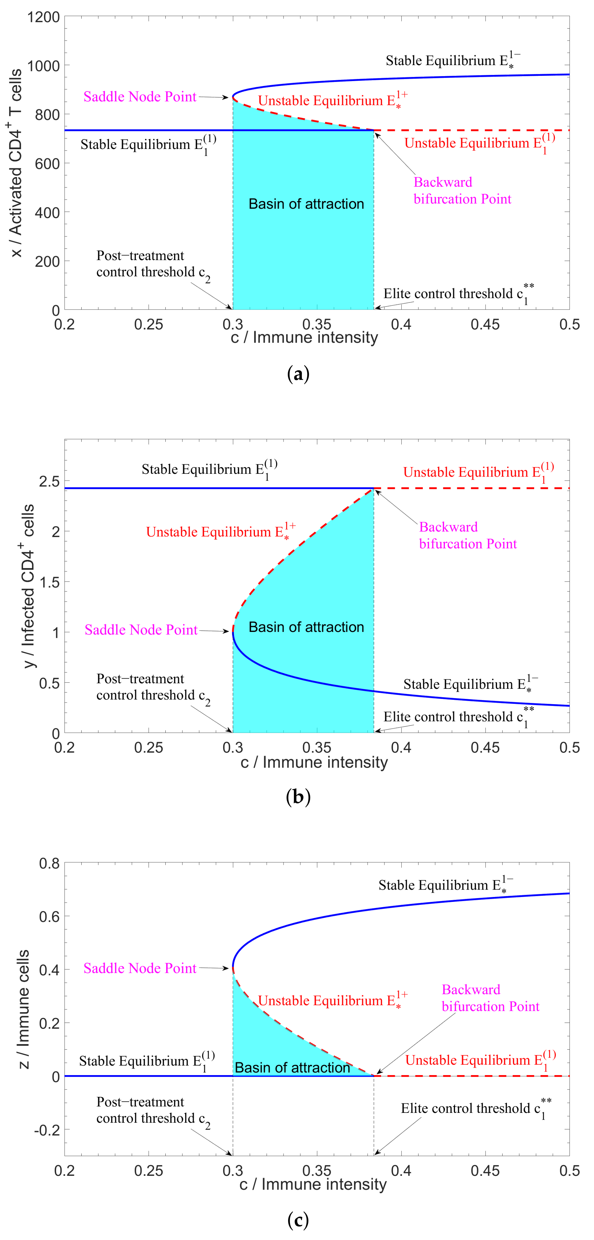
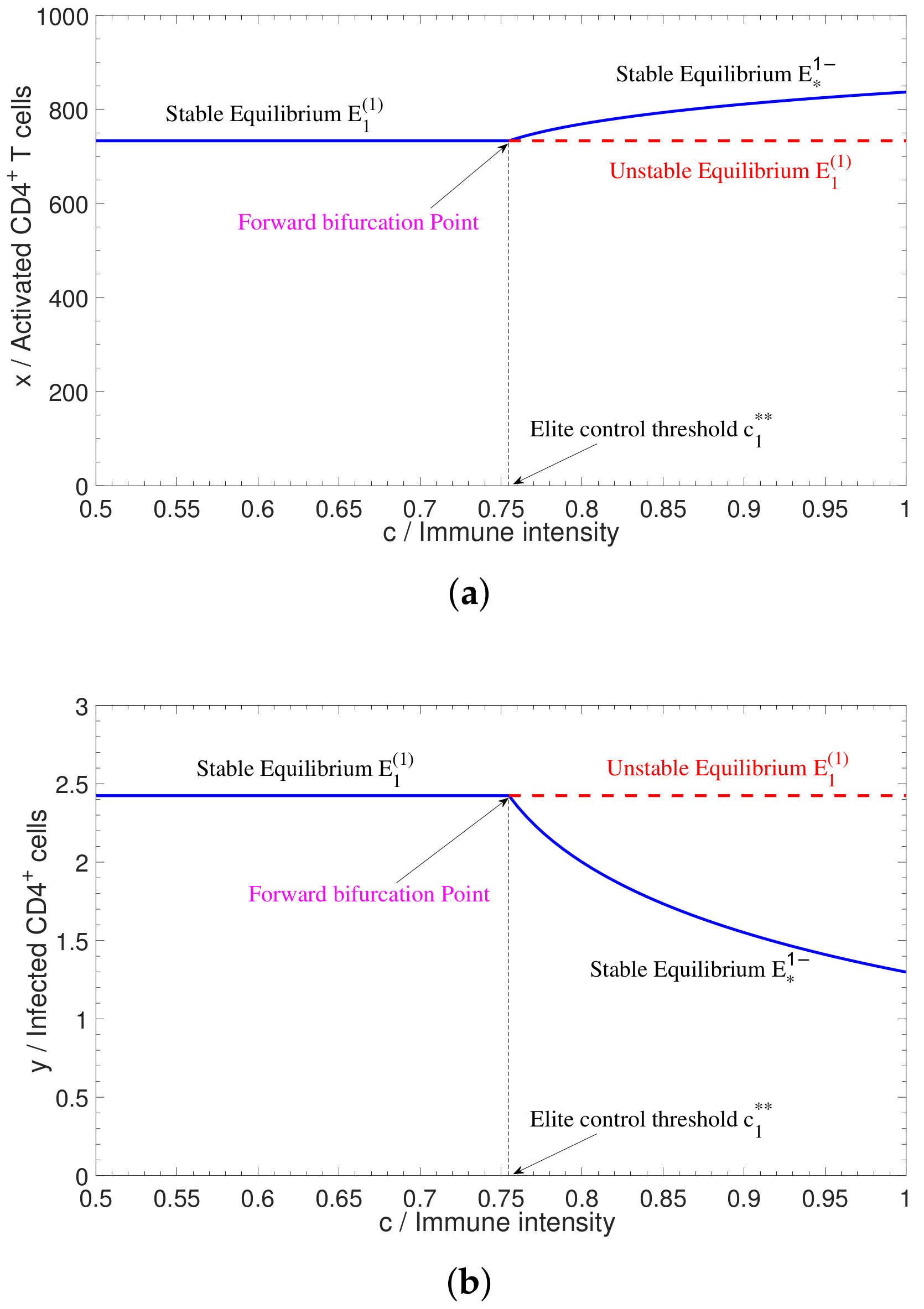
2.1. Bifurcations in Three-Dimensional Model

In this section, we prove the existence of backward and forward bifurcations in system (1) using the theorem developed by Castillo-Chavez and Song [24]. From the results in [1], let $\tilde{E}$ be any arbitrary equilibrium of system (1). The Jacobian matrix associated with system (1) is

$$J_1=\left[\begin{array}{ccc}-d-\beta (1-ϵ)y& -\beta (1-ϵ)x& 0\\ \beta (1-ϵ)y& \beta (1-ϵ)x-a-pz& -py\\ 0& \frac{c\alpha z-cz{y}^2}{{(\alpha +\gamma y+y^2)}^2}& \frac{cy}{\alpha +\gamma y+y^2}-b\end{array}\right].$$

The characteristic equation of the linearized system of (1) at $\tilde{E}$ is given by $\parallel \lambda I-J_1\parallel =0$.

Theorem 1.

If $R_0^{\left(1\right)}>R_c^{\left(1\right)}>1$ and $c=c_1^{**}$, then system (1) undergoes a backward bifurcation at $E_1^{\left(1\right)}$. Here, c is the bifurcation parameter.

Proof. 

From Theorem 3.10 in [1], we know that $Det\left[J_{E_1^{\left(1\right)}}\right]=0$ and zero is a simple eigenvalue of $J_{E_1^{\left(1\right)}}$. Here, $J=J_1$. Let $v={(v_1,v_2,v_3)}^T$ and $w=(w_1,w_2,w_3)$ denote the right eigenvector and the left eigenvector of $J_{E_1^{\left(1\right)}}$ corresponding to the zero eigenvalue, respectively. Then, we can find a right eigenvector associated with zero eigenvalue, given by

$$v={\left(1,\frac{-d-\beta (1-ϵ)y_1^{\left(1\right)}}{\beta (1-ϵ)x_1^{\left(1\right)}},\frac{\beta (1-ϵ)}{p}\right)}^T.$$

The left eigenvector is given by $w=(0,0,1)$ from Theorem 3.10 in [1]. Let $(x,y,z)=(x_1,x_2,x_3)$ and $G={(g_1,g_2,g_3)}^T$. From the proof of Theorem 3.10 [1], we have

$$\begin{array}{ccc}\hfill D{G}_c(E_1^{\left(1\right)};c_1^{**})v& \triangleq & \left[\begin{array}{c}\sum _{i=1}^3{v}_i\frac{{\partial }^2{g}_1}{\partial x_i\partial c}(E_1^{\left(1\right)},c_1^{**})\\ \sum _{i=1}^3{v}_i\frac{{\partial }^2{g}_2}{\partial x_i\partial c}(E_1^{\left(1\right)},c_1^{**})\\ \sum _{i=1}^3{v}_i\frac{{\partial }^2{g}_3}{\partial x_i\partial c}(E_1^{\left(1\right)},c_1^{**})\end{array}\right]\hfill \\ & =& {\left[\begin{array}{ccc}0& 0& 0\\ 0& 0& 0\\ 0& \frac{(\alpha -y^2)z}{{(\alpha +\gamma y+y^2)}^2}& \frac{y}{\alpha +\gamma y+y^2}\end{array}\right]}_{(E_1^{\left(1\right)};c_1^{**})}\left[\begin{array}{c}1\\ \frac{-d-\beta (1-ϵ)y_1^{\left(1\right)}}{\beta (1-ϵ)x_1^{\left(1\right)}}\\ \frac{\beta (1-ϵ)}{p}\end{array}\right]\hfill \\ & =& \left[\begin{array}{c}0\\ 0\\ \frac{\beta (1-ϵ)y_1^{\left(1\right)}}{p\left(\alpha +\gamma y_1^{\left(1\right)}+{\left(y_1^{\left(1\right)}\right)}^2\right)}\end{array}\right],\hfill \end{array}$$

$$\begin{array}{cc}\hfill D^{2}G(E_1^{\left(1\right)};c_1^{**})(v,v)& \triangleq \left[\begin{array}{c}\sum _{i,j=1}^3{v}_i\frac{{\partial }^2{g}_1}{\partial x_i\partial x_j}(E_1^{\left(1\right)},c_1^{**})\\ \sum _{i,j=1}^3{v}_i\frac{{\partial }^2{g}_2}{\partial x_i\partial x_j}(E_1^{\left(1\right)},c_1^{**})\\ \sum _{i,j=1}^3{v}_i\frac{{\partial }^2{g}_3}{\partial x_i\partial x_j}(E_1^{\left(1\right)},c_1^{**})\end{array}\right]\hfill \\ & ={\left[\begin{array}{c}\frac{2(d+\beta (1-ϵ\left)y\right)}{x}\\ 0\\ \frac{-2cz(3\alpha y+\alpha \gamma -y^3)}{{(\alpha +\gamma y+y^2)}^3}\frac{{(d+\beta (1-ϵ)y)}^2}{{\left(\beta (1-ϵ)x\right)}^2}-\frac{2c(\alpha -y^2)(d+\beta (1-ϵ)y)}{p{(\alpha +\gamma y+y^2)}^{2}x}\end{array}\right]}_{(E_1^{\left(1\right)};c_1^{**})}\hfill \\ & =\left[\begin{array}{c}\frac{2\left(d+\beta (1-ϵ)y_1^{\left(1\right)}\right)}{x_1^{\left(1\right)}}\\ 0\\ -\frac{2c_1^{**}\left(\alpha -{\left(y_1^{\left(1\right)}\right)}^2\right)\left(d+\beta (1-ϵ)y_1^{\left(1\right)}\right)}{p{\left(\alpha +\gamma y_1^{\left(1\right)}+{\left(y_1^{\left(1\right)}\right)}^2\right)}^2{x}_1^{\left(1\right)}}\end{array}\right].\hfill \end{array}$$

Therefore,

$$\begin{array}{cc}\hfill b& =w·\left[D{G}_c(E_1^{\left(1\right)};c_1^{**})v\right]=\frac{\beta (1-ϵ)y_1^{\left(1\right)}}{p\left(\alpha +\gamma y_1^{\left(1\right)}+{\left(y_1^{\left(1\right)}\right)}^2\right)},\hfill \\ \hfill a& =w·\left[D^{2}G(E_1^{\left(1\right)};c_1^{**})(v,v)\right]=-\frac{2c_1^{**}\left(\alpha -{\left(y_1^{\left(1\right)}\right)}^2\right)\left(d+\beta (1-ϵ)y_1^{\left(1\right)}\right)}{p{\left(\alpha +\gamma y_1^{\left(1\right)}+{\left(y_1^{\left(1\right)}\right)}^2\right)}^2{x}_1^{\left(1\right)}}.\hfill \end{array}$$

We know that, when $R_0^{\left(1\right)}>R_c^{\left(1\right)}$ and $c=c_1^{**}$, we have $y_1^{\left(1\right)}>\sqrt{\alpha }$ from [1]. Then, $b>0$ and $\alpha -{\left(y_1^{\left(1\right)}\right)}^2<0$, implying that $a>0$. Therefore, according to Corollary 4.1 in [24], both a and b are positive, implying that system (1) undergoes a backward bifurcation at $c=c_1^{**}$. Here, c is the bifurcation parameter.  □

Remark 1.

Suppose $R_0^{\left(1\right)}>R_c^{\left(1\right)}>1$. From Table 3 in [24], we can see that, when the vertical axis represents z (Immune cells) and x (Activated CD$4^{+}$ T cells), the bifurcation diagrams are drawn in Figure 1a,c. Considering Remark 1 in [24], if we choose

$$v={\left(-1,\frac{d+\beta (1-ϵ)y_1^{\left(1\right)}}{\beta (1-ϵ)x_1^{\left(1\right)}},-\frac{\beta (1-ϵ)}{p}\right)}^{T}andw=\left(0,0,-\frac{p}{\beta (1-ϵ)}\right),$$

then we can find $a<0$ and $b>0$ by calculation. Thus, when the vertical axis represents y (Infected CD$4^{+}$ T cells), the bifurcation diagram is drawn in Figure 1b.

When $1<R_0^{\left(1\right)}<R_c^{\left(1\right)}$, there also exists forward bifurcation in system (1), which will be proven in the following.

Theorem 2.

If $1<R_0^{\left(1\right)}<R_c^{\left(1\right)}$ and $c=c_1^{**}$, then system (1) undergoes a forward bifurcation at $E_1^{\left(1\right)}$. Here, c is the bifurcation parameter.

Proof. 

We know that, when $1<R_0^{\left(1\right)}<R_c^{\left(1\right)}$ and $c=c_1^{**}$, $y_1^{\left(1\right)}<\sqrt{\alpha }$ from [1]. Then, we can find that

$$b=\frac{\beta (1-ϵ)y_1^{\left(1\right)}}{p\left(\alpha +\gamma y_1^{\left(1\right)}+{\left(y_1^{\left(1\right)}\right)}^2\right)}>0$$

and

$$a=-\frac{2c_1^{**}\left(\alpha -{\left(y_1^{\left(1\right)}\right)}^2\right)\left(d+\beta (1-ϵ)y_1^{\left(1\right)}\right)}{p{\left(\alpha +\gamma y_1^{\left(1\right)}+{\left(y_1^{\left(1\right)}\right)}^2\right)}^2{x}_1^{\left(1\right)}}<0.$$

Therefore, according to Theorem 4.1 in [24], we know that, when $a<0$ and $b>0$, system (1) undergoes a forward bifurcation at $c=c_1^{**}$. Here, c is the bifurcation parameter.  □

Remark 2.

Suppose $1<R_0^{\left(1\right)}<R_c^{\left(1\right)}$. From Table 3 in [24], we can see that the vertical axis represents z (Immune cells) and x (Activated CD$4^{+}$ T cells) in the bifurcation diagrams plotted in Figure 2a,c. Considering Remark 1 in [24], if we choose

$$v={\left(-1,\frac{d+\beta (1-ϵ)y_1^{\left(1\right)}}{\beta (1-ϵ)x_1^{\left(1\right)}},-\frac{\beta (1-ϵ)}{p}\right)}^T\mathrm{and}w=\left(0,0,-\frac{p}{\beta (1-ϵ)}\right),$$

then we can find $a>0$ and $b>0$. Thus, when the vertical axis represents y (Infected CD$4^{+}$ T cells), the bifurcation diagram is plotted in Figure 2b.

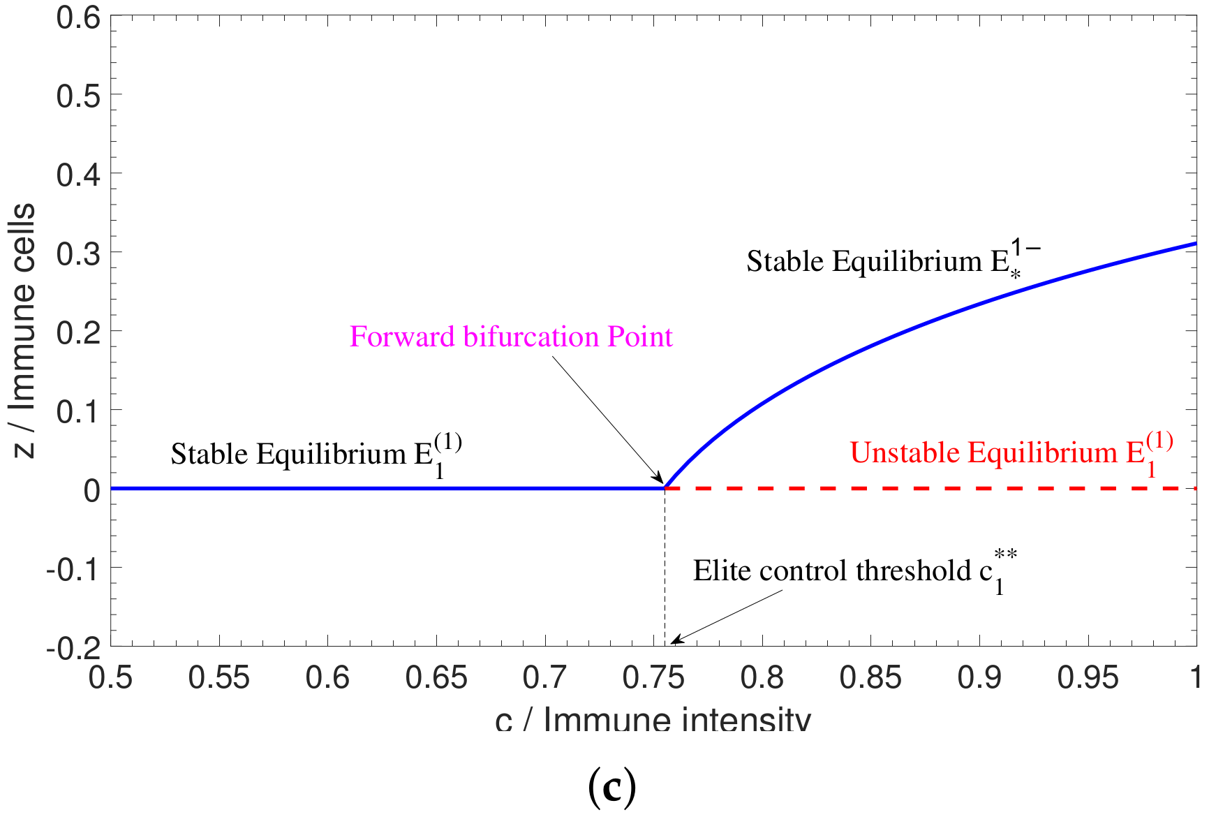
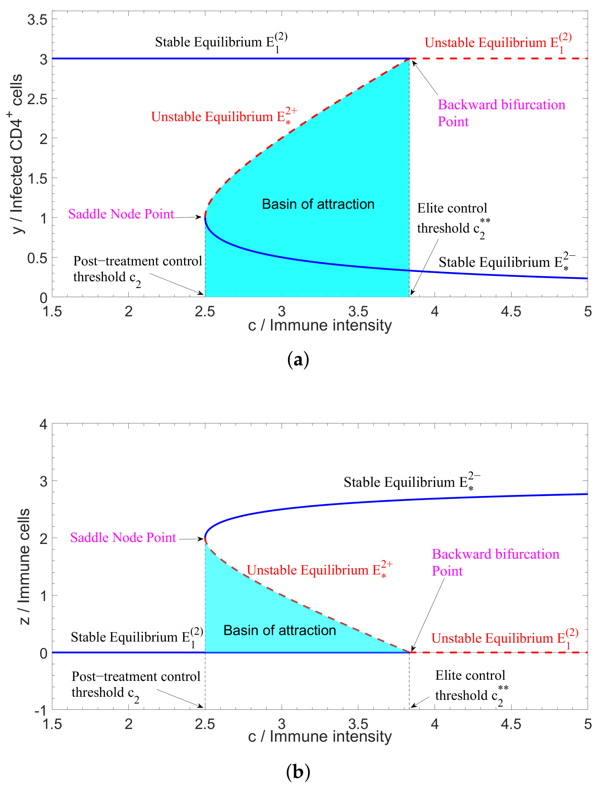
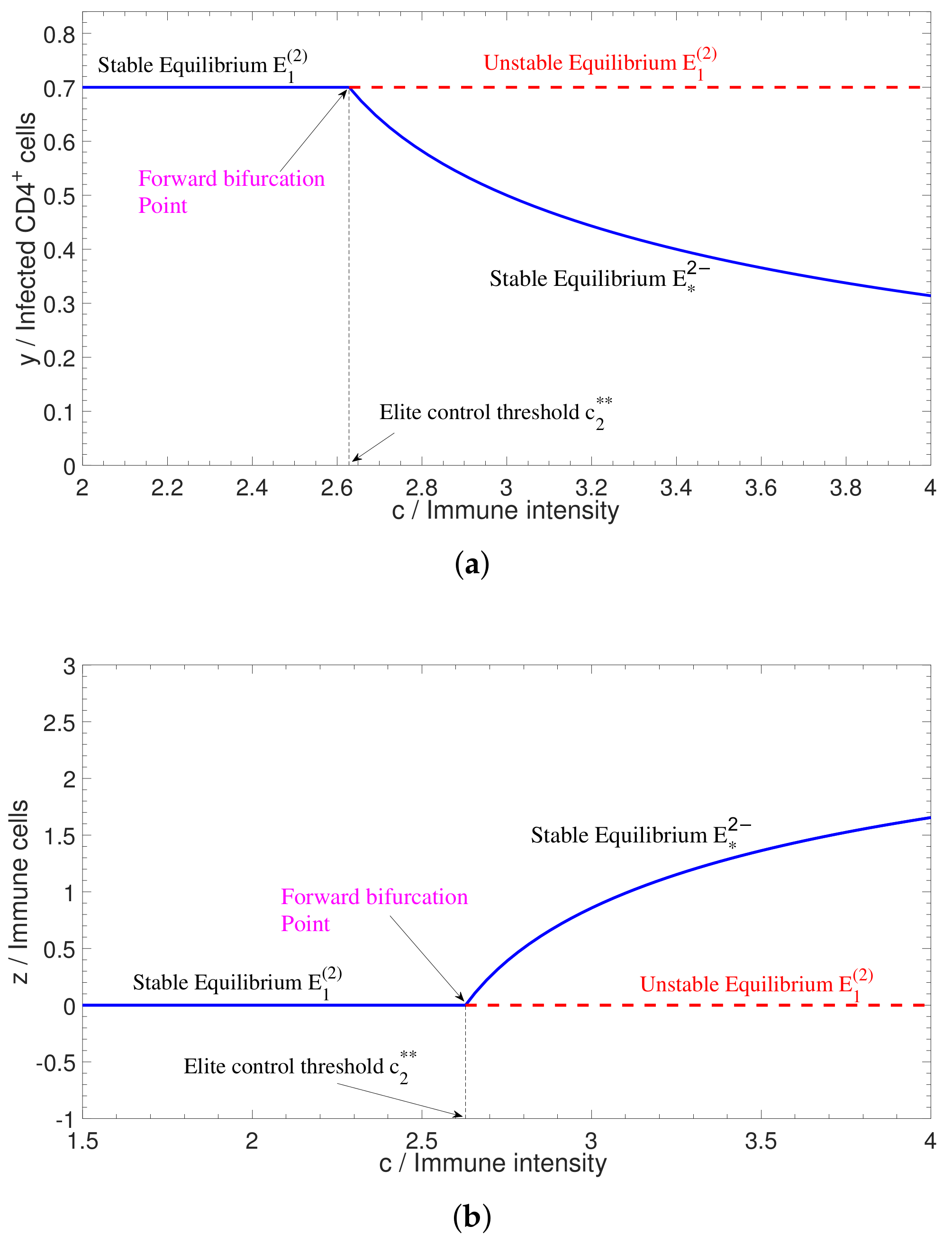
2.2. Bifurcations in Two-Dimensional Model

In this section, we use the same method to prove the existence of backward bifurcation in system (2). From the results in [1], let $\tilde{E}$ be any arbitrary equilibrium of system (2). The Jacobian matrix associated with the system (2) is

$$J_2=\left[\begin{array}{cc}r-a-\frac{2\gamma }{K}y-pz& -py\\ \frac{(\alpha -y^2)cz}{{(\alpha +\gamma y+y^2)}^2}& \frac{cy}{\alpha +\gamma y+y^2}-b\end{array}\right].$$

The characteristic equation of the linearized system of (2) at $\tilde{E}$ is given by $\parallel \lambda I-J_2\parallel =0$.

Theorem 3.

If $R_0^{\left(2\right)}>R_c^{\left(2\right)}>1$ and $c=c_2^{**}$, then system (2) undergoes a backward bifurcation at $E_1^{\left(2\right)}$. Here, c is the bifurcation parameter.

Proof. 

From Theorem 5.11 in [1], we know that $Det\left[J_{E_1^{\left(2\right)}}\right]=0$ and zero is a simple eigenvalue of $J_{E_1^{\left(2\right)}}$. Here, $J=J_2$. Let $\xi ={({\xi }_1,{\xi }_2)}^T$ and $\theta =({\theta }_1,{\theta }_2)$ denote the right eigenvector and left eigenvector of $J_{E_1^{\left(2\right)}}$ corresponding to the zero eigenvalue, respectively. Then, the right eigenvector associated with 0 eigenvalue is $\xi ={(-\frac{pK}{r},1)}^T$, and the left eigenvector $\theta$ is $\theta =(0,1)$. Let $F={(P_2,Q_2)}^T$. From the proof of Theorem 5.11 in [1], we can find

$$\begin{array}{ccc}\hfill D{F}_c(E_1^{\left(2\right)};c_2^{**})\xi & =& \left[\begin{array}{cc}0& 0\\ \frac{(\alpha -y^2)z}{{(\alpha +\gamma y+y^2)}^2}& \frac{y}{\alpha +\gamma y+y^2}\end{array}\right]{\left[\begin{array}{c}-\frac{pK}{r}\\ 1\end{array}\right]}_{(E_1^{\left(2\right)};c_2^{**})}\hfill \\ & =& \left[\begin{array}{c}0\\ \frac{y_1^{\left(2\right)}}{\alpha +\gamma y_1^{\left(2\right)}+{\left(y_1^{\left(2\right)}\right)}^2}\end{array}\right]\hfill \end{array}$$

and

$$\begin{array}{ccc}\hfill D^{2}F(E_1^{\left(2\right)};c_2^{**})(\xi ,\xi )& =& {\left[\begin{array}{c}0\\ \frac{-2cz(3\alpha y+\alpha \gamma -y^3)}{{(\alpha +\gamma y+y^2)}^3}-\frac{2c\gamma (\alpha -y^2)}{pK{(\alpha +\gamma y+y^2)}^2}\end{array}\right]}_{(E_1^{\left(2\right)};c_2^{**})}\hfill \\ & =& \left[\begin{array}{c}0\\ -\frac{2\gamma c_2^{**}{(\alpha -(y_1^{\left(2\right)})}^2)}{{(\alpha +\gamma y_1^{\left(2\right)}+{\left(y_1^{\left(2\right)}\right)}^2)}^{2}pK}\end{array}\right].\hfill \end{array}$$

Therefore,

$$\begin{array}{cc}\hfill b=& \theta ·\left[D{F}_c(E_1^{\left(2\right)};c_2^{**})\xi \right]=\frac{y_1^{\left(2\right)}}{\alpha +\gamma y_1^{\left(2\right)}+{\left(y_1^{\left(2\right)}\right)}^2},\hfill \\ \hfill a=& \theta ·\left[D^{2}F(E_1^{\left(2\right)};c_2^{**})(v,v)\right]=-\frac{2pK{c}_2^{**}pK\left(\alpha -{\left(y_1^{\left(2\right)}\right)}^2\right)}{r{\left(\alpha +\gamma y_1^{\left(2\right)}+{\left(y_1^{\left(2\right)}\right)}^2\right)}^2}.\hfill \end{array}$$

We know that, when $R_0^{\left(2\right)}>R_c^{\left(2\right)}>1$ and $c=c_2^{**}$, we have $y_1^{\left(2\right)}>\sqrt{\alpha }$ from [1]. Thus, it is clear that $b>0$ and $\alpha -{\left(y_1^{\left(2\right)}\right)}^2<0$ implying that $a>0$. Therefore, according to Corollary 4.1 in [24], both a and b are positive, implying that system (2) undergoes a backward bifurcation at $c=c_1^{**}$. Here, c is the bifurcation parameter.  □

Remark 3.

Suppose $R_0^{\left(2\right)}>R_c^{\left(2\right)}$. From Table 3 in [24], we can see that, when the vertical axis represents z (Immune cells), the bifurcation diagram is plotted in Figure 3b. Considering Remark 1 in [24], if we choose $\xi ={(1,-\frac{r}{pK})}^T$ and $\theta =(0,-\frac{pK}{r})$, then we can find $a<0$ and $b>0$ by calculation. Thus, the vertical axis represents y (Infected CD$4^{+}$ T cells) in the bifurcation diagram plotted in Figure 3a.

Theorem 4.

If $1<R_0^{\left(2\right)}<R_c^{\left(2\right)}$ and $c=c_2^{**}$, then system (2) undergoes a forward bifurcation at $E_1^{\left(2\right)}$. Here, c is the bifurcation parameter.

Proof. 

We use the same method as Theorem 2 and the results in Theorem 3. When $1<R_0^{\left(2\right)}<R_c^{\left(2\right)}$ and $c=c_2^{**}$, we have $y_1^{\left(2\right)}>\sqrt{\alpha }$, then

$$b=\frac{y_1^{\left(2\right)}}{\alpha +\gamma y_1^{\left(2\right)}+{\left(y_1^{\left(2\right)}\right)}^2}>0$$

and

$$a=-\frac{2pK{c}_2^{**}pK\left(\alpha -{\left(y_1^{\left(2\right)}\right)}^2\right)}{r{\left(\alpha +\gamma y_1^{\left(2\right)}+{\left(y_1^{\left(2\right)}\right)}^2\right)}^2}<0.$$

Therefore, according to Theorem 4.1 in [24], we know that, when $a<0$ and $b>0$, system (2) undergoes a forward bifurcation at $c=c_2^{**}$. Here, c is the bifurcation parameter.  □

Remark 4.

Suppose $1<R_0^{\left(2\right)}<R_c^{\left(2\right)}$. From Table 3 in [24], we can see that the vertical axis represents z (Immune cells), and the bifurcation diagram is plotted in Figure 4b. Considering Remark 1 in [24], if we choose $\xi ={(1,-\frac{r}{pK})}^T$ and $\theta =(0,-\frac{pK}{r})$, then we can find $a>0$ and $b>0$ by calculation. Thus, the vertical axis represents y (Infected CD$4^{+}$ T cells), and the bifurcation diagram is plotted in Figure 4a.

3. Robustness for Bistable System

When a system with backward bifurcation is bistable, it has two basins of attraction. Robustness is one of the fundamental characteristics of biological systems. A general definition of the robustness for biological systems can be used: robustness, the ability to maintain performance in the face of perturbations and uncertainty, is a long-recognized key property of living systems [25].

According to the general definition, we propose the definition of robustness for bistable systems, which is measured by the area of the basin of attraction, namely the definite integral of positive steady solution curve on the bistable interval. The robustness corresponding to x, y and z for bistable system (1) can be calculated by

$$\begin{array}{ccc}\hfill R_x^{\left(1\right)}& =& {\int }_{c_2}^{c_1^{**}}{x}_{*}^{1+}dc\hfill \\ & =& {\int }_{c_2}^{c_1^{**}}\frac{s}{(1-ϵ)\beta y_{*}^{1+}+d}dc,\hfill \\ \hfill R_y^{\left(1\right)}& =& {\int }_{c_2}^{c_1^{**}}{y}_{*}^{1+}dc\hfill \\ & =& {\int }_{c_2}^{c_1^{**}}\frac{c-\gamma b\pm \sqrt{{(\gamma b-c)}^2-4\alpha b^2}}{2b}dc,\hfill \\ \hfill R_z^{\left(1\right)}& =& {\int }_{c_2}^{c_1^{**}}{z}_{*}^{1+}dc.\hfill \end{array}$$

As shown in Figure 1, the area covered by cyan denotes $R_x^{\left(1\right)}$(a), $R_y^{\left(1\right)}$(b) and $R_z^{\left(1\right)}$(c), the robustness for bistable system (1) corresponding to x, y and z, respectively. Here, we use the default parameter in Table 3, and we can calculate $R_x^{\left(1\right)}\approx 65.5722$, $R_y^{\left(1\right)}\approx 0.1553$ and $R_z^{\left(1\right)}\approx 0.0126$.

Using the same method, we can define the robustness corresponding to y and z for bistable system (2) as follows

$$\begin{array}{ccc}\hfill R_y^{\left(2\right)}& =& {\int }_{c_2}^{c_2^{**}}{y}_{*}^{2+}dc\hfill \\ & =& {\int }_{c_2}^{c_2^{**}}\frac{c-\gamma b\pm \sqrt{{(\gamma b-c)}^2-4\alpha b^2}}{2b}dc,\hfill \\ \hfill R_z^{\left(2\right)}& =& {\int }_{c_2}^{c_2^{**}}{z}_{*}^{2+}dc.\hfill \end{array}$$

Then, the area covered by cyan in Figure 3 denotes $R_y^{\left(2\right)}$(a) and $R_z^{\left(2\right)}$(b), the robustness for bistable system (2) corresponding to y and z, respectively. Here, we use the default parameter in

Table 4. Description and values of the parameters in model (2).

Symbol	Description	Value	Reference
r	Growth rate of infected cells	$6{\mathrm{day}}^{-1}$	–
K	Environmental carrying capacity of infected cells	–	–
a	Death rate of cells	$3{\mathrm{day}}^{-1}$	–
p	Killing rate of infected CD$4^{+}$ T cells by immune cells	$1{\mathrm{day}}^{-1}$	–
c	immune intensity	$3{\mathrm{day}}^{-1}$	–
$\alpha$	Constant in nonmonotonic immune response	1 cells/μL	–
$\gamma$	Constant in nonmonotonic immune response	1 cells/μL	–
b	Death rate of immune cells	$1{\mathrm{day}}^{-1}$	–

, and we can calculate $R_y^{\left(2\right)}\approx 2.9014$ and $R_z^{\left(2\right)}\approx 1.0986$.

When the system has some parameter and initial value perturbations, if the parameter and initial values are always in one basin of attraction, then the system will maintain its performance. However, if the parameter and initial values change the basin of attraction to another due to the perturbations, then the system will appear to have a regime shift and change the original performance. Thus, the larger the attraction is, the more difficult to find a regime shift. Considering systems (1) and (2), we can think of robustness $R_x^{\left(1\right)}$, $R_y^{\left(1\right)}\left(R_y^{\left(2\right)}\right)$ and $R_z^{\left(1\right)}\left(R_z^{\left(2\right)}\right)$ as the difficulty of virus rebound, the greater $R_y^{\left(1\right)}\left(R_y^{\left(2\right)}\right)$ is, the better robustness for bistable system, and then the tumor cells have greater difficulty in rebounding. However, the greater $R_x^{\left(1\right)}$ and $R_z^{\left(1\right)}\left(R_z^{\left(2\right)}\right)$ are, the easier the system to be in the steady state of high virus load—that is, the virus can rebound more easily.

4. Sensitive Analysis and Numerical Simulations

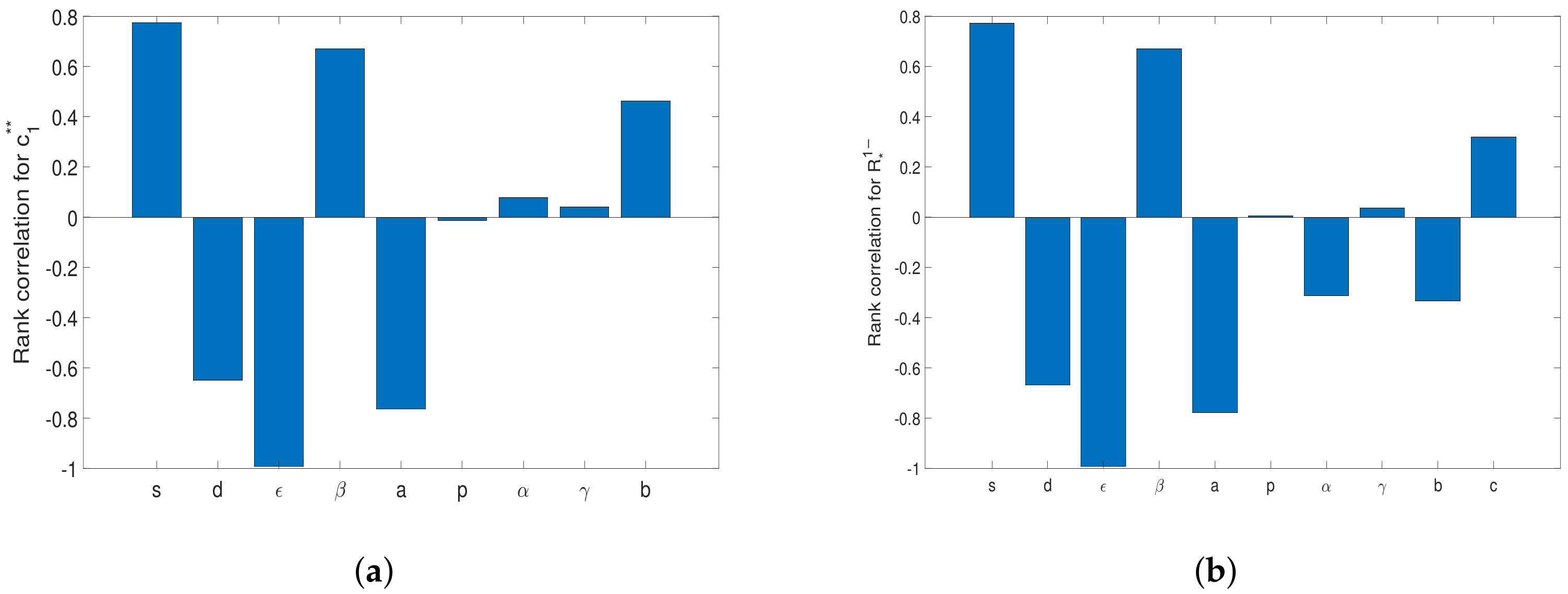
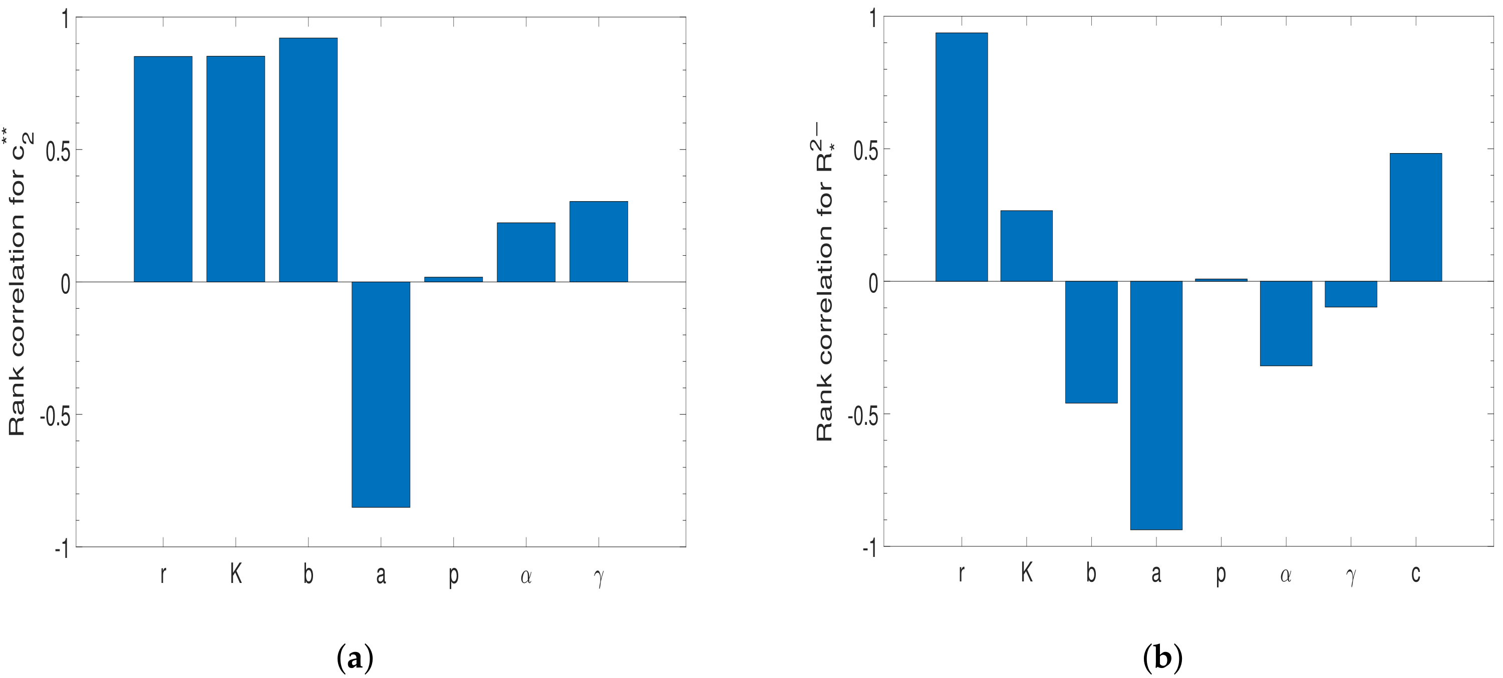
4.1. Sensitive Analysis

Sensitive analysis is an important method to test the influence of parameter variations on system dynamics [26]. In the following, we conduct sensitive analysis with the aim of revealing the relationship between the elite control threshold and the basic immune reproduction number and system parameters in our model (1) and model (2). Here, we use Latin hypercube sampling (LHS) and partial rank correlation coefficients (PRCCs) [27,28] to test the dependence of $c_1^{**}$, $c_2^{**}$ and $R_{*}^{1-}$, $R_{*}^{2-}$. As a statistical sampling method, LHS provides an efficient analysis of parameter variations across simultaneous uncertainty ranges in each parameter [27].

PRCC, on the other hand, shows the level of significance for each parameter. The PRCC is obtained using the rank transformed LHS matrix and output matrix [28]. We performed 4000 simulations per run and used a uniform distribution function to test for the significance of PRCCs for all parameters with wide ranges. When $\left|PRCC\right|>0.4$, there was a significant correlation between the input parameters and output variables. For $\left|PRCC\right|\in (0.2,0.4]$, the correlations were moderate. When $\left|PRCC\right|\in [0,0.2]$, we had weak correlations.

The PRCC results in Figure 5 illustrate the dependence of $c_1^{**}$ and $R_{*}^{1-}$ on each parameter in system (1). Furthermore, Figure 6 illustrates the dependence of $c_2^{**}$ and $R_{*}^{2-}$ on each system parameter in system (2).

From Figure 5 for system model (1), we notice that the generated rate of CD$4^{+}$ T cells s, the death rate of CD$4^{+}$ T cells d, the infected rate $\beta$, the treatment rate $ϵ$, the death rate of infected cells a and the death rate of immune cells b have significant influences on the exile control threshold $c_1^{**}$; and the generated rate of CD$4^{+}$ T cells s, the death rate of CD$4^{+}$ T cells d, the infected rate $\beta$, the treatment rate $ϵ$ and the death rate of infected cells a have significant influences on the basic immune reproduction number $R_{*}^{1-}$. From Figure 6 for system model (2), the growth rate of infected cells r, the environmental capacity K, the death rate of immune cells b and the death rate of infected cells a have significant influences on the exile control threshold $c_2^{**}$; and the growth rate of infected cells r, the death rate of immune cells b, the death rate of infected cells a and the immune intensity c have significant influences on the basic immune reproduction number $R_{*}^{2-}$.

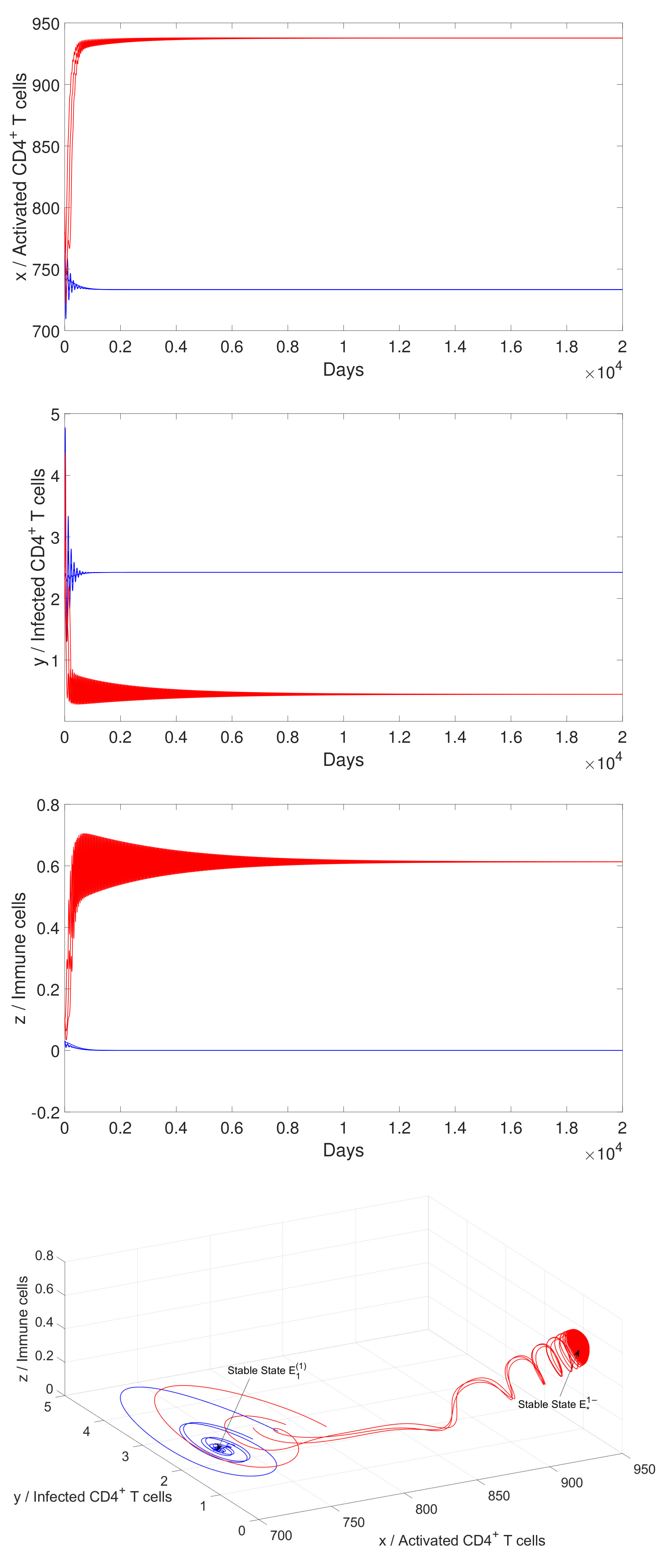
4.2. Numerical Simulation

In this section, we perform numerical simulations to verify our analytical results. We perform numerical simulations for system (1) using the default parameters in Table 3.

Table 3. Description and values of the parameters in model (1).

Symbol	Description	Value	Reference
s	Production rate of CD$4^{+}$ T cells	10 cells/μL/day	[29]
d	Death rate of CD$4^{+}$ T cells	$0.01{\mathrm{day}}^{-1}$	[29]
$ϵ$	Drug efficacy	0.9	–
$\beta$	Infection rate of CD$4^{+}$ T cells	0.015 cells/μL/day	[6]
a	Death rate of infected cells	$1.1{\mathrm{day}}^{-1}$	–
p	Killing rate of infected CD$4^{+}$ T cells by immune cells	$0.5{\mathrm{day}}^{-1}$	–
c	immune intensity	$0.3{\mathrm{day}}^{-1}$	–
$\alpha$	Constant in nonmonotonic immune response	1 cells/μL	–
$\gamma$	Constant in nonmonotonic immune response	1 cells/μL	–
b	Death rate of immune cells	$0.1{\mathrm{day}}^{-1}$	–

Table 3. Description and values of the parameters in model (1).

Symbol	Description	Value	Reference
s	Production rate of CD$4^{+}$ T cells	10 cells/μL/day	[29]
d	Death rate of CD$4^{+}$ T cells	$0.01{\mathrm{day}}^{-1}$	[29]
$ϵ$	Drug efficacy	0.9	–
$\beta$	Infection rate of CD$4^{+}$ T cells	0.015 cells/μL/day	[6]
a	Death rate of infected cells	$1.1{\mathrm{day}}^{-1}$	–
p	Killing rate of infected CD$4^{+}$ T cells by immune cells	$0.5{\mathrm{day}}^{-1}$	–
c	immune intensity	$0.3{\mathrm{day}}^{-1}$	–
$\alpha$	Constant in nonmonotonic immune response	1 cells/μL	–
$\gamma$	Constant in nonmonotonic immune response	1 cells/μL	–
b	Death rate of immune cells	$0.1{\mathrm{day}}^{-1}$	–

Then, the thresholds $R_0^{\left(1\right)}\approx 1.3636$, $c_2=0.3$ and $c_1^{**}\approx 0.3837$. In this case, when we choose $c_2<c=0.37<c_1^{**}$ and different initial values, both the immune-free equilibrium $E_1^{\left(1\right)}$ and the positive equilibrium $E_{*}^{1-}$ are stable (see Figure 7), and system (1) appears bistable. When we choose $c=0.65>c_1^{**}$ and different initial values, only the positive equilibrium $E_{*}^{1-}$ is stable (see Figure 8). If we choose $\alpha =10$ cells/μL, then $R_0^{\left(1\right)}\approx 1.3636$, $R_c^{\left(1\right)}\approx 1.4743>R_0^{\left(1\right)}$, $c_2=0.3$ and $c_1^{**}\approx 0.7549$. In this case, when we choose $c=0.8>c_1^{**}$ and different initial values, only the immune-free equilibrium $E_1^{\left(1\right)}$ is stable (see Figure 9). When we choose $c=0.7<c_1^{**}$ and different initial values, only the positive equilibrium $E_{*}^{1-}$ is stable (see Figure 10). Figure 7, Figure 8, Figure 9 and Figure 10 verify the results in Figure 1 and Figure 2.

We perform numerical simulations for system (2). We use the default parameters in Table 4.

If we choose $K=6$ cells/μL, then the thresholds $R_0^{\left(2\right)}=2$, $R_c^{\left(2\right)}\approx 1.3333<R_0^{\left(2\right)}$, $c_2=2.5$, and $c_2^{**}\approx 3.8333$. In this case, when we choose $c_2<c=3<c_2^{**}$ and different initial values, both the immune-free equilibrium $E_1^{\left(2\right)}$ and the positive equilibrium $E_{*}^{2-}$ are stable (see Figure 11a). When we choose $c=4>c_1^{**}$ and different initial values, only the positive equilibrium $E_{*}^{2-}$ is stable (see Figure 11b). If we choose K = 1.4 cells/μL and different initial values, then $R_0^{\left(2\right)}=2$, $R_c^{\left(2\right)}\approx 2.4286>R_0^{\left(2\right)}$, $c_2^{**}\approx 2.6286$. In this case, when we choose $c=2.5<c_2^{**}$ and different initial values, only the immune-free equilibrium $E_1^{\left(2\right)}$ is stable (see Figure 12a). When we choose $c=2.7>c_1^{**}$ and different initial values, only the positive equilibrium $E_{*}^{2-}$ is stable (see Figure 12b). Figure 11 and Figure 12 verify the results in Figure 3 and Figure 4.

5. Discussion

In this paper, we found that the nonmonotonic immune responses in the viral infection systems in [1] undergo backward and forward bifurcation at the elite control threshold if we select the immune intensity as the bifurcation parameter under different conditions. When the immune intensity is less than the elite control threshold, the viral load will be under control or rebound. Only when the immune intensity is greater than the elite control threshold will the viral load be under elite control. Such concepts can be applied to the dynamics of infection and immunity of EBV, HIV and SARS-CoV2.

The results show that a combination of antiviral therapy and immunotherapy may contribute to the functional cure of HIV, that is, the immune intensity is greater than the elite control threshold through immunotherapy. Then, with long term control of viral replication and low viral load, a functional cure of HIV can be realized. The HIV patients under elite control still need to be cautious and continue to receive immunotherapy. If the immune intensity is less than the post-treatment control threshold, the virus can rebound again.

References

1. Wang, S.; Li, H.; Xu, F. Monotomic and nonmonotonic immune responses in viral infection systems. Discrete Cont. Dyn-B 2022, 27, 141–165. [Google Scholar] [CrossRef]
2. Wang, S.; Xu, F. Thresholds and bistability in virus-immune dynamics. Appl. Math. Lett. 2018, 78, 105–111. [Google Scholar] [CrossRef]
3. Wang, S.; Xu, F.; Rong, L. Bistability analysis of an hiv model with immune response. J. Biol. Syst. 2017, 25, 677–695. [Google Scholar] [CrossRef]
4. Wang, S.; Xu, F. Analysis of an HIV model with post-treatment control. J. Appl. Anal. Comput. 2020, 10, 667–685. [Google Scholar] [CrossRef]
5. Wang, X.; Tan, Y.; Cai, Y.; Wang, K.; Wang, W. Dynamics of a stochastic HBV infection model with cell-to-cell transmission and immune response. Math. Biosci. Eng. 2020, 18, 616–642. [Google Scholar] [CrossRef] [PubMed]
6. Conway, J.; Perelson, A. Post-treatment control of HIV infection. Proc. Natl. Acad. Sci. USA 2015, 112, 5467. [Google Scholar] [CrossRef] [PubMed] [Green Version]
7. Wang, X.; Tan, Y.; Cai, Y.; Wang, K.; Wang, W. Dynamics of a delayed integro-differential HIV infection model with multiple target cells and nonlocal dispersal. Eur. Phys. J. Plus 2021, 136, 117. [Google Scholar]
8. Bi, K.; Chen, Y.; Zhao, S.; Ben-Arieh, D.; Wu, C.H.J. A new zoonotic visceral leishmaniasis dynamic transmission model with age-structure. Chaos Solitons Fractals 2020, 133, 109622. [Google Scholar] [CrossRef]
9. AlAgha, A.; Elaiw, A. Stability of a general reaction-diffusion HIV-1 dynamics model with humoral immunity. Eur. Phys. J. Plus 2019, 134, 390. [Google Scholar] [CrossRef]
10. Wang, W.; Ma, W.; Feng, Z. Dynamics of reaction–diffusion equations for modeling CD4+ T cells decline with general infection mechanism and distinct dispersal rates. Nonlinear Anal. RWA 2020, 51, 102976. [Google Scholar] [CrossRef]
11. Ruan, S.; Xiao, D. Global analysis in a predator-prey system with nonmonotonic function response. SIAM J. Appl. Math. 2000, 61, 1445–1472. [Google Scholar]
12. Wang, S.; Wang, X.; Wu, X. Bifurcation analysis for a food chain model with nonmonotonic nutrition conversion rate of predator to top predator. Int. J. Bifurcat. Chaos 2020, 30, 2050113. [Google Scholar] [CrossRef]
13. Lu, M.; Huang, J.; Ruan, S.; Yu, P. Bifurcation analysis of an SIRS epidemic model with a generalized nonmonotone and saturated incidence rate. J. Differ. Equ. 2019, 267, 1859–1898. [Google Scholar] [CrossRef] [PubMed]
14. Lu, M.; Huang, J.; Ruan, S.; Yu, P. Global dynamics of a susceptible-infectious-recovered epidemic model with a generalized nonmonotone incidence rate. J. Dyn. Differ. Equ. 2020, 33, 1625. [Google Scholar] [CrossRef]
15. Andrews, J.F. A mathematical model for the continuous culture of microorganisms utilizing inhibitory substrates. Biotechnol. Bioeng. 1968, 10, 707–723. [Google Scholar] [CrossRef]
16. Xie, X.; Ma, J.; van den Driessche, P. Backward bifurcation in within-host HIV models. Math. Biosci. 2021, 335, 108569. [Google Scholar] [CrossRef]
17. van den Driessche, P.; Watmough, J. A simple SIS epidemic model with a backward bifurcation. J. Math. Biol. 2000, 40, 525–540. [Google Scholar] [CrossRef]
18. Bi, K.; Chen, Y.; Wu, C.H.J.; Ben-Arieh, D. A memetic algorithm for solving optimal control problems of Zika virus epidemic with equilibriums and backward bifurcation analysis. Commun. Nonlinear Sci. Numer. Simul. 2020, 84, 105176. [Google Scholar] [CrossRef]
19. Chen, Y.; Bi, K.; Zhao, S.; Ben-Arieh, D.; Wu, C.H.J. Modeling individual fear factor with optimal control in a disease-dynamic system. Chaos Solitons Fractals 2017, 104, 531–545. [Google Scholar] [CrossRef]
20. Zhao, S.; Kuang, Y.; Wu, C.H.; Ben-Arieh, D.; Ramalho-Ortigao, M.; Bi, K. Zoonotic visceral leishmaniasis transmission: Modeling, backward bifurcation, and optimal control. J. Math. Biol. 2016, 73, 1525–1560. [Google Scholar] [CrossRef]
21. Bi, K.; Chen, Y.; Wu, C.H.J.; Ben-Arieh, D. Learning-based impulse control with event-triggered conditions for an epidemic dynamic system. Commun. Nonlinear Sci. Numer. Simul. 2022, 108, 106204. [Google Scholar] [CrossRef]
22. Garba, S.M.; Gumel, A.B.; Bakar, M.A. Backward bifurcations in dengue transmission dynamics. Math. Biosci. 2008, 215, 11–25. [Google Scholar] [CrossRef] [PubMed]
23. van den Driessche, P.; Watmough, J. Reproduction numbers and sub-threshold endemic equilibria for compartmental models of disease transmission. Math. Biosci. 2002, 180, 29–48. [Google Scholar] [CrossRef]
24. Castillo-Chavez, C.; Song, B. Dynamical models of tuberculosis and their applications. Math. Biosci. Eng. 2004, 1, 361–404. [Google Scholar] [CrossRef]
25. Kitano, H. Towards a theory of biological robustness. Mol. Syst. Biol. 2007, 3, 137. [Google Scholar] [CrossRef]
26. Xiao, Y.; Tang, S.; Zhou, Y.; Smith, R.; Wu, J.; Wang, N. Predicting the HIV/AIDS epidemic and measuring the effect of mobility in mainland China. J. Theor. Biol. 2013, 317, 271–285. [Google Scholar] [CrossRef]
27. Blower, S.; Dowlatabadi, H. Sensitivity and uncertainty analysis of complex models of disease transmission: An HIV model, as an example. Int. Stat. Rev. 1994, 2, 229–243. [Google Scholar] [CrossRef]
28. Marino, S.; Hogue, I.; Ray, C.; Kirschner, D. A methodology for performing global uncertainty and sensitivity analysis in systems biology. J. Theor. Biol. 2008, 254, 178–196. [Google Scholar] [CrossRef] [Green Version]
29. Bonhoeffer, S.; Rembiszewski, M.; Ortiz, G.; Nixon, D. Risks and benefits of structured antiretroviral drug therapy interruptions in HIV-1 infection. AIDS 2000, 14, 2313–2322. [Google Scholar] [CrossRef]
Figure 1. Bifurcation diagrams of system (1) where the vertical axis represents Activated CD 4 + T cells (see (a)), Infected CD 4 + T cells (see (b)) and Immune cells (see (c)). The parameter values are listed in Table 3. The solid line represents stable equilibria, and the dotted line represents unstable equilibria. The post-treatment control threshold is c 2 0.3 , the elite control threshold is c * * 0.3837 , and the bistable interval is ( 0.3 , 0.3837 ) .
Mathematics 10 02139 g001
Figure 2. Bifurcation diagrams of system (1) where the vertical axis represents Activated CD 4 + T cells (see (a)), Infected CD 4 + T cells (see (b)) and Immune cells (see (c)). The parameter values are listed in Table 3 and α = 10 . The solid line represents stable equilibria, and the dotted line represents unstable equilibria. The elite control threshold is c 1 * * 0.7549 .
Mathematics 10 02139 g002aMathematics 10 02139 g002b
Figure 3. Bifurcation diagrams of system (2) where the vertical axis represents Infected CD 4 + T cells (see (a)) and Immune cells (see (b)). The parameter values are listed in Table 4 and K = 6 cells/μL. The solid line represents stable equilibria, and the dotted line represents unstable equilibria. The post-treatment control threshold is c 2 2.5 , the elite control threshold c 2 * * 3.8333 , and the bistable interval is ( 2.5 , 3.8333 ) .
Mathematics 10 02139 g003
Figure 4. Bifurcation diagrams of system (2) where the vertical axis represents Infected CD 4 + T cells (see (a)) and Immune cells (see (b)). The parameter values are listed in Table 4 and K = 1.4 cells/μL. The solid line represents stable equilibria, and the dotted line represents unstable equilibria. The elite control threshold c 2 * * 2.6286 .
Mathematics 10 02139 g004
Figure 5. Partial rank correlation coefficients illustrating the dependence of c 1 * * (a) and R * 1 (b) for the system (1) on each parameter. The parameter values are listed in Table 3.
Mathematics 10 02139 g005
Figure 6. Partial rank correlation coefficients illustrating the dependence of c 2 * * (a) and R * 2 (b) for the system (2) on each parameter. The parameter values are listed in Table 4.
Mathematics 10 02139 g006
Figure 7. Time histories and trajectories of system (1) with different initial values for c = 0.37 day 1 . E 1 ( 1 ) and E * 1 are stable. System (1) shows the bistable phenomenon. Other parameter values are listed in Table 3.
Mathematics 10 02139 g007
Figure 8. Time histories and trajectories of system (1) with different initial values for c = 0.65 day 1 . Only E * 1 is stable. Other parameter values are listed in Table 3.
Mathematics 10 02139 g008
Figure 9. Time histories and trajectories of system (1) with different initial values for c = 0.7 day 1 . Only E 1 ( 1 ) is stable. Other parameter values are listed in Table 3 and α = 10 .
Mathematics 10 02139 g009
Figure 10. Time histories and trajectories of system (1) with different initial values for c = 0.8 day 1 . Only E * 1 is stable. Other parameter values are listed in Table 3 and α = 10 .
Mathematics 10 02139 g010
Figure 11. Trajectories of system (2) with different initial values for c = 3 day 1 and c = 4 day 1 . When c = 3 day 1 , E 1 ( 2 ) and E * 2 are stable. System (2) shows the bistable phenomenon (see (a)). When c = 4 day 1 , only E * 2 is stable (see (b)). Other parameter values are listed in Table 4 and K = 6 cells/μL.
Mathematics 10 02139 g011
Figure 12. Trajectories of system (2) with different initial values for c = 2.5 day 1 and c = 2.7 day 1 . When c = 2.5 day 1 , only E 1 ( 2 ) is stable (see (a)). When c = 2.7 day 1 , only E * 2 is stable (see (b)). Other parameter values are listed in Table 4 and K = 1.4 cells/μL.
Mathematics 10 02139 g012