Article

A Stochastic Optimization Algorithm to Enhance Controllers of Photovoltaic Systems

1
Research Unit of Photovoltaic, Wind and Geothermal Systems, National Engineering School of Gabès, University of Gabès, Gabès 6029, Tunisia
2
Department of Computer Science, College of Computer Science and Engineering, University of Hail, Hail 1234, Saudi Arabia
3
Department of Industrial Engineering, College of Engineering, University of Hail, Hail 1234, Saudi Arabia
4
Department of Electrical Engineering, College of Engineering, University of Hail, Hail 1234, Saudi Arabia
5
School of Industrial Engineering, Pontificia Universidad Católica de Valparaíso, Valparaíso 2362807, Chile
*
Authors to whom correspondence should be addressed.
Mathematics 2022, 10(12), 2128; https://doi.org/10.3390/math10122128
Submission received: 17 May 2022 / Revised: 12 June 2022 / Accepted: 14 June 2022 / Published: 19 June 2022
(This article belongs to the Section Computational and Applied Mathematics)

Abstract

:
Increasing energy needs, pollution of nature, and eventual depletion of resources have prompted humanity to obtain new technologies and produce energy using clean sources and renewables. In this paper, we design an advanced method to improve the performance of a sliding mode controller combined with control theory for a photovoltaic system. Specifically, we decouple the controlled output of the system from any perturbation source and assess the effectiveness of the results in terms of solution quality, closed-loop control stability, and dynamical convergence of the state variables. This study focuses on the climatic conditions that may affect the behavior of a solar energy plant to supply a motor with the highest possible efficiency and nominal operating conditions. The designed method enables us to obtain an optimal performance by means of advanced control techniques and a slime mould stochastic optimization algorithm. The efficiency and performance of this method are examined based on a benchmark model of a photovoltaic system via numerical analysis and simulation.

1. Introduction

Increasing global energy needs, pollution of nature, and eventual depletion of fossil fuels have prompted humanity to explore new technologies to produce electrical energy using clean sources and renewables, such as solar and wind power [1,2]. However, systems based on wind or solar energies are not stable due to seasonal and daily variations. Indeed, renewable energy systems utilizing a single intermittent source, such as a photovoltaic (PV) system or wind energy, are not stable due to these variations [3,4,5].
PV systems present problems related to nonlinear characteristics and energy production that depends on climatic conditions which are highly random. Therefore, the design of an optimized PV system becomes difficult. Consequently, the development of efficient techniques to overcome these problems is of paramount importance [6,7].
The use of intelligent techniques [8,9,10] is currently experiencing a great boom in complex and ill-defined systems for their modeling, optimization, identification, and control. This is a product of their adaptability to changes in system parameters and their robustness in response to disturbances, as well as to modeling errors.
Intelligent techniques are a viable and efficient solution to the problem of optimizing PV systems [8,9]. The literature shows that these systems and metaheuristic techniques are highly related to each other in several research areas. Indeed, metaheuristic optimization techniques have been implemented in problems of parameter determination for solar PV systems [1]. In addition, they have been utilized in problems of maximum power point tracking techniques for PV plants subjected to partial shading conditions and random disturbances [9,10]. Moreover, they have been used in problems of heuristic operation strategy [4], problems of power control and energy management and storage [6], as well as in problems of advanced control for grid-connected PV systems [1,5]. One can combine analytical and metaheuristic methods to enhance the performance and features of a PV generation source mainly used in a remote area.
Thus, intelligent, innovative methods are of interest and widely employed. Their utilization enables us to improve the efficiency of PV systems and provide better performance than those obtained with classical algorithms. This can be conducted regardless of the variation in climatic conditions (such as sunshine and temperature), even in the most severe and unfavorable cases. One can propose a technique that combines intelligent slime mould optimization (SMO), feedback linearization (FBL), and sliding mode control (SMC) with different architectures and metaheuristic optimization algorithms.
The SMC is one of the techniques that are applied to solve the problem of parametric variation. This controller ensures a zero static error, guarantees a fast response, and obtains a stable, robust system [10,11,12,13]. Its main fields of application are robotics [14,15,16] and control of electric machines [17,18,19,20]. The SMC is considered one of the best ordering approaches for nonlinear systems due to its multiple advantages. They include high precision, fast dynamic response, stability, simplicity of the design and implementation, as well as robustness with respect to variation of internal/external parameters [20,21,22]. However, the SMC has some disadvantages, such as the appearance of chattering caused by the corresponding discontinuous part, which can have a detrimental effect on the actuators. Furthermore, with the SMC, the system is always subject to high control to ensure its convergence to the desired state, which is not desirable [23,24,25,26].
Among the solutions proposed to problems of parametric variation, we can mention the control stated by a sliding mode band limit, which consists of replacing the switching function with a saturation. Nevertheless, this solution is only a special case of the SMC. Hence, there exists an interest in using a control method that combines FBL and SMC to achieve a sturdy and smooth drive.
To obtain the control input, the gains are optimized by an intelligent SMO. The SMO is one of the approaches that have been most explored to improve the capacities of learning systems and combine different systems for the same task. Nonetheless, to the best of our knowledge, the use of a stochastic SMO method for determining the controller gains of a PV system has not been explored until now.
The main objective of this study is to design an advanced approach for solving the problem of improving the efficiency of an SMC combined with FBL control theory in a PV system. Specifically, we decouple the controlled output of the system from any perturbation sources and assess the results’ effectiveness in terms of solution quality, closed-loop control stability, and dynamical convergence of the state variables. We focus on climatic conditions that can affect the behavior of a solar energy plant to extract the maximum power supplied by a PV generator at the highest possible efficiency. This approach allows an optimal performance to be obtained using advanced control techniques and an SMO algorithm. We examine efficiency and performance of this approach utilizing a benchmark model of a PV system via numerical analysis and simulation.
Therefore, the main contributions of the designed approach originate from the benefits of employing the capability of the SMO to have adaptive weights in its process of searching for the global optimum. This impacts the accuracy of the controller gain selection and attenuates the chattering of the SMC. Closed-loop system stability is guaranteed with a well-filtered voltage feeding the motor direct current (DC) pump load.
The novelty of the present work can be summarized in the following points:
(i)
The FBL, used as a main control technique, is implemented to enable high local performance.
(ii)
The SMC technique is then combined with the FBL to attenuate the effects of random and matched disturbances. This combination is expected to improve the dynamic performance of the controlled system.
(iii)
Due to the uncertainties in the model, it is impossible to fully eliminate the disturbances utilizing only the conventional SMC. To overcome this problem, a method associated with an SMO technique is implemented to allow fine-tuning of the controller gains ensuring the efficiency of the PV system as a stand-alone power generator in a remote area.
In terms of PV process benefits, the designed approach aims at preserving the nominal operating condition for the DC motor pump, while considering a varying irradiance during the day coupled with a random environmental disturbance and a matched electric default.
After this introduction, the paper is structured as follows. In Section 2, some elementary characteristics of input–output FBL (I/O FBL) and SMC are presented. In addition, in this section, to strengthen the tracking controller, an advanced nonlinear control strategy that combines I/O FBL and SMC is introduced. In Section 3, the fundamentals of the SMO algorithm are provided. Section 4 is dedicated to the application of the above approaches to a PV system. Concluding remarks and perspectives of our work are given in Section 5.

2. Background and Problem Formulation

2.1. Robust Nonlinear Control Strategy

The basic factors concerning the I/O FBL technique can be found in [27,28,29]. Further information, regarding the structural specifications of this technique, may be sourced by referring to [30,31,32].
Generally, the standard formula of a nonlinear system is expressed as
{ X ˙ = F ( X ) + G ( X )   U + Υ ( X )   D , y = H ( X ) ,
where X   ϵ   n is the state vector; U   ϵ   is the control input; y   ϵ   is the output; D   ϵ   m is the disturbance; F : n n , G : n n , and Υ : m n represent vector fields; and H :   n is a function, with denoting infinitely differentiable functions.
Definition 1 
([30]). The system stated in (1) is assumed to have a local relative degree denoted by r at an operating point X 0 if:
(i)
L G L F k H ( X ) = 0 , for all X around X 0 and for all k < r 1 ;
(ii)
L G L F r 1 H ( X 0 ) 0 ,
where L F k H ( X ) denotes the k-th Lie differential operator of the scalar field H ( X ) with respect to the vector field F ( X ) .
If a system has a finite relative degree, the determination of a state variable coordinate transformation, denoted by Z = Φ ( X ) , is achievable through consecutive differentiations of the output. In the altered coordinates, the system can be formulated in a regular arrangement. When disturbances are not part of the model, the conventional form generates a controllability canonical form given by
{ Z 1 ˙ = Z 2 = L F H ( X ) , Z ˙ 2 = Z 3 = L F 2 H ( X ) , Z ˙ r 1 = Z r = L F r 1 H ( X ) , Z ˙ r = v , Z ˙ i = ϑ ( Z ) ,   r + 1 i n , y = Z 1 = H ( X ) ,
where v defined in (2) is the new control (external) input of the equivalent linear system and Z = [ Π 1 Π 2 ] T , with “T” denoting the transpose of a matrix, Π 1 = [ H ( X ) L F H ( X ) L F 2 H ( X ) L F r 1 H ( X ) ] and Π 2 = [ ψ 1 ( X ) ψ n r ( X ) ] being the dynamic compensator, such that ψ 1 ( X ) , …, ψ n r ( X ) are variables that can be determined by solving the equations stated as
ψ i ( X ) X ,   G ( X ) = L G ψ i ( X ) = 0 ,   i   ϵ   { 1 , , n r } .
The reader can consult [29] for further details on the compensator characteristics.
Note that if r < n , the system seems to decompose into a linear sub-system with dimension r (which is attributable to the I/O performance) and a nonlinear sub-system of dimension n r (whose activity does not have influence over the output). This nonlinear sub-system is considered a zero dynamic linear system.
For a system with a local relative degree to be I/O linearized, it must be at the minimum phase, with the zero dynamics being asymptotically constant. Observe that the configuration of the feedback control law is determined by the characteristics of the problem. To decouple the output from measurable fluctuations [14,33,34,35,36], external inputs are considered, giving rise to the relative degree concept, regarding the disturbances.
Definition 2 
([30]). The relative degree c i of the output y ( t ) , in relation to the disturbance, is expressed as the least integer c i such that
L Υ L F c i 1 H ( X ) 0 .
The array of measurable disturbances can be categorized as follows [14]:
(i)
When c i > r , the impact of the disturbance is not as straightforward as the control input, with c i being given in (4). The entire information from the disturbance is accessible through the system states, and as such, the decoupling of y ( t ) from the disturbance D is rendered unnecessary.
(ii)
When c i = r , the disturbance and control input have a similar influence on the system output, and feedforward performance is essential to perform decoupling.
(iii)
When c i < r , the disturbance influences the output more straightforwardly than the control output. Some form of predictive activity is required to perform disturbance rejection.
It is considered ideal that the output y ( t ) tracks some reference signal. As indicated by the coordinate transformation [27,28,29,30,31,32], the control input U defined in (1) is determined as
U = v L F r H ( X ) L G L F r 1 H ( X ) + T ( X , D ) ,
where T ( X , D ) expressed in (5) is an analytic component (that will be defined in the next theorem) and that serves to decouple the output from the measured disturbances; and υ represents, as mentioned in (2), an external input that can be employed to design precise features for eigenvalues of the closed-loop system. Consequently, this external input is defined as
v = K Z = [ K 1 K n ] Z ,
where K represents the linear controller gain vector. The decoupling function T ( X , D ) is acquired from the principal outcomes [14], which are summarized in the following theorem. Comprehensive outcomes are provided in [14].
Theorem 1 
([14]). Consider the nonlinear system stated in (1) and assume c i to be the relative degree specified in Definition 2. Then, the function T ( X , D )   that facilitates the independence of y ( t ) from D is formulated as
T ( X , D ) = 1 L G L F r 1 H ( X ) k = 0 r c i d k d t k ( L Υ L F r k 1 H ( X ) D ) .
Note that PV modeling involves two main stages. First, the electrical model of the PV cell is devised. Then, second, by an approximation of the values of the different parameters, this model is postulated. Next, we describe the PV models and corresponding formulations of the problems to conduct their optimization.

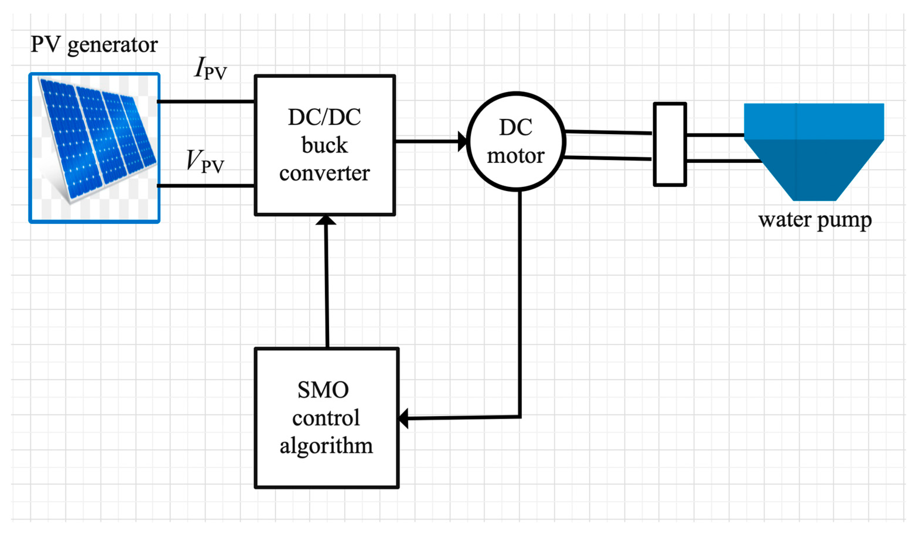
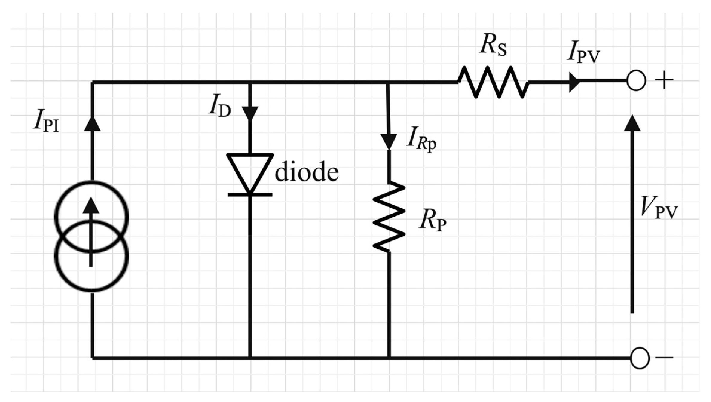
2.2. PV Model Description

In what follows, we present an efficient system for pumping water, which is straightforwardly attached to a PV system. Figure 1 portrays the fundamental block diagram of the examined PV system. This water pumping system comes with a PV generator, a DC/DC buck converter, and a DC motor pump.
Now, we formulate the model of the PV generator. A diode model is frequently utilized to describe the electric behavior of a PV cell (or generator). In this model, an electric generator represents the PV cell. The generator is comparable to a current source parallel to a diode. Like a junction diode, the current–voltage connection is nonlinear in nature [37,38]. It also contains a shunt parallel resistance R P originating from tiny electric shorts through the PN junction of the PV cell and small series resistance R S simulating the internal losses of the PV module. (Note that a PN junction is an interface or a boundary between two semiconductor material types, namely P and N types, inside a semiconductor.) In Figure 2, the Kirchhoff law is applied. The output current I is obtained by the expression stated as
I PV = I PI I D I R P ,
where I PI is the photocurrent, I D is the current of the diode, and I R P is the current flowing in the parallel resistor, which can be computed as
I R P = V PV + R S   I PV R P ,
which is proportional to the saturation current and where V PV represents the PV generator input voltage. An equation formulated as
I D = I SD ( exp ( q ( V PV + R S   I PV ) n   K B   T ) 1 )
expresses the value of this magnitude, where I SD is the reverse saturation single diode current in amperes (A), q is the electron charge (1.6 × 0−19 C), K B is the Boltzmann constant (1.38 × 10⁻²³ J/K), T is the cell temperature in Kelvin degrees (°K), and n is the ideality factor of the diode. Replacing the expressions given in (9) and (10) in (8), we obtain
I PV = I PI I SD ( exp ( q ( V PV + R S   I PV ) n   T   K B   ) 1 ) V PV + R S   I PV R P .
Note that the photocurrent depends mainly on the solar radiation and operating temperature of the cell, as described by
I PI = ( I SC + K I ( T T ref ) ) E E ref ,  
where I SC is the short-circuit current of the cell at standard test conditions (25 °C and 1000 W/m2), K I is the temperature coefficient of the cell short-circuiting current, T ref is the reference temperature of the cell (in °K, with °K = 25 °C + 273), E is the solar radiation in (W/m2), and E ref is the reference insolation of the cell, which is equal to 1000 W/m2. In addition, the cell saturation current varies with the temperature of the cell, which is described as
I SD = I R S ( T T ref ) exp ( q   E G ( T T ref 1 T ) / ( n   K B ) ) ,
where I R S is the reverse saturation current of the PV cell and E G is the gap energy of the semiconductor used in the PV cell (in eV). The reverse saturation current is given by
I R S = I sc exp ( q   V oc n   T   K B   N S ) 1 ,
where V OC is the open-circuit voltage and N S is the number of cells connected in series.
Next, the buck converter model is formulated. The solar generator, which is a nonlinear mechanism, is only capable of delivering maximum power, at precise levels of voltage and current. To compel the delivery of maximum power, from the PV generator to the load, the DC–DC buck converter is integrated between the PV generator and DC motor pump. The PV array presented in Figure 3 is a group of several PV modules electrically connected in series ( N S cells) and in parallel ( N p columns) to generate the required current and voltage. Accordingly, the current–voltage (IV) characteristic equation of a PV module becomes stated as
I PV = N P   I PI N P   I SD ( exp ( q ( V PV N S + R S   I PV N P   ) n   K B   T ) 1 ) N P   V PV N S + R S R P .
Table 1 reports the parameters of the PV module used in this work. The PV and IV characteristics are represented in Figure 4.
The buck converter comprises a power transistor ( S T ) and a free-wheeling diode ( S D ). The power transistor S T is engaged as a switch, which is turned on and off intermittently by an external driver circuit of pulse width modulation. The establishment of the average output voltage is achieved through an expression given by
V A = ρ   V PV ,
where V A is the DC–DC converter voltage, related to armature, that is identical to the system output voltage (DC motor feeding voltage), while ρ is the duty cycle of the switch S T , with 0 < ρ < 1 also being an alterable turn ratio. As deduced from the formula given in (16), control of the output voltage is achievable through alterations in the chopper duty cycle ρ . Note that the pulse width modulation is employed to fluctuate ρ [39,40,41]. The supply power (PV power) is deemed equivalent to the load power if less loss is assumed. Then, we have
V A I A = V PV   I P ,
and
V PV V A = I A   I P = ρ ,
where I A is the armature current. Observe that the expressions stated in (17) and (18) evolve such that the chopper can be regarded as a DC transformer, with an alterable turn ratio ρ , and a PV generator output current I A that supplies the DC motor load.
Next, the model of the DC motor pump is formulated. The DC motor is the simplest form of a permanent magnet machine. Assume that, for each operating point (disregarding the magnetic reaction), the flux remains consistent. With respect to the DC machine model, R and L depict the armature resistance and inductance, respectively. The transference of energy, from the electrical component towards the mechanical component, corresponds to the proportionality between the finite element E a and the angular speed Ω stated as
E A = K B   Ω .
The DC motor propels a centrifugal pump, which, for the purpose of simplification, is expressed as a torque Γ proportional to the angular speed given by
Γ = K T   Ω ,
where K T stated in (20) is a torque constant.

2.3. Nonlinear Control Design

Here, we formulate and synthesize an analytical second-order SMC of a PV water pumping system. The recommended procedure is derived from a state feedback controller, which is centered on a linearizing conversion of the closed-loop system.
The I/O FBL is the basis for the nonlinear controller, which is dependent on differentiations in the output of interest, until the input is straightforwardly linked to an offshoot of the output. This facilitates the commencement of a linearization [27,28].
A differential geometry-based procedure is employed to calculate the control variable (duty cycle of the DC–DC converter) by means of the following:
(i)
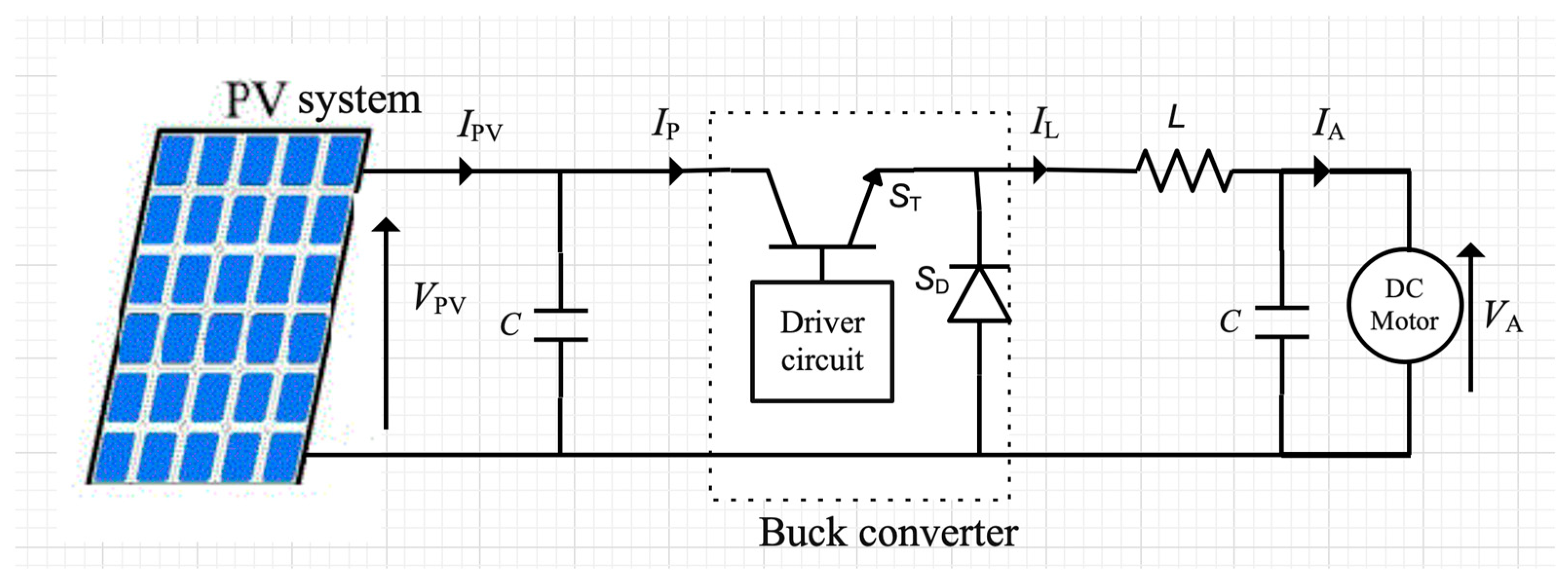
Determining the PV system’s state space equations [38,39] as
{ I ˙ A = V A L K B L Ω R L I A + d 1 ,   Ω ˙ = K B J I A K T + F J Ω d 2 ,   I ˙ L = V A L + V PV L ( U sin ( V A ) ) ,   V ˙ A = I L C V A R   C ,  
where C is a capacitor, L is an inductor, I L is the inductor current, and the mechanical losses are denoted by torques J and F in (21), which indicate the DC machine’s inertia and viscous friction coefficients, respectively; U = ρ ; J is also the motor’s moment of inertia; and d 1 ,   d 2 , and d 3 denote random disturbance vector components.
(ii)
Expressing the system in the conventional standard configuration given by
{ X ˙ = F ( X ) + G ( X )   U + Υ ( X ) D , y = H ( X ) ,  
where X stated in (22) is defined as
X = [ X 1 X 2 X 3 X 4 ] = [ I A Ω I L V A ] ,
which denotes the state vector that considers the motor current, motor angular position, inductance current, and DC motor supply voltage. In addition, we have that
F ( X ) = [ V A L K B L Ω R L I A K B J I A K T + F J Ω   V A L V PV L sin ( V A )   I L C V A R   C   ] ,   G ( X ) = [ 0 0 V PV L 0 ] ,
Υ ( X ) = [ 1 0 0 0 0 1 0 0 0 0 1 0 0 0 0 0 ] , D = [ d 1 d 2 d 3 0 ] ,   U = ρ ,   y = H ( X ) = V A .
(iii)
Stating R = 1.072   Ω and L = 0.05 H , which denote the armature resistance and inductance, as mentioned, respectively; J = 476 × 10 6   kg   m 2 and F = 88 × 10 5   m 2 / s , which denote the DC machine’s inertia and viscous friction coefficients, as also mentioned, respectively; and C = 4000 × 10 6   F , which represents the capacitor, as mentioned.
(iv)
Computing the relative degree r by deriving y up to the point, when the control variable U materializes to equations given by
{ y = V A ,   y ˙ = V ˙ A = I L C V A R   C ,   y ¨ = V ¨ A = 1 L   C V A + V PV L   C U V PV L 2 sin ( V A ) 1 C d 3 1 R   C ( I L C V A R   C ) ,
which is attained from r  = 2 . Note that this approach emphasizes developing a control output that promotes the capacity of the PV system for output trajectory tracking, as well as for disturbance decoupling.
(v)
Expressing the input controller as
U = L   C   v + V A + L R ( I L   C V A R   C ) + L 2   sin ( V A ) V PV + T ( X , D ) ,
where v is the control input.
As the relative degree of disturbance is nil, which is below the system’s relative degree, it follows that the disturbance influences the output more straightforwardly than the control output. This brings the need for some form of predictive activity to perform disturbance rejection. Nevertheless, this control method is hampered by the fact that only local effectiveness is guaranteed. Note that, so far, both modeling defects and parameter variability are not considered. There are indications that this method generates globally vigorous outputs under parametric ambiguity, as well as disturbance upon integration with the sliding mode formalism [14]. In the following section, we delve into control approaches based on the second-order sliding mode (SOSM) technique to achieve a significantly dynamic output tracking quality.

3. Linearization, Sliding Modes, and Control Input Synthesis Methodology

3.1. Input/Output Linearization and Second-Order Sliding Modes

The downside to the control technique recommended above has to do with the fact that only local robustness is assured. In addition, note that, at this point, both modeling inaccuracies and parameter ambiguities are not considered. It is taken for granted that the nonlinear conversion is precisely identified and that all states are obtainable. The recommended technique is expected to bring in more globally vigorous results if it is merged with SMC [11,12,13]. This considers the issue of unmeasured disturbances and states to arrive at a solution for the I/O linearization problem. However, it is known that in a situation where certain disturbances and states are unmeasured, disturbance rejection may not be performed, although bounding of the output may still occur. We recommend that an SOSM technique [10], in a nonlinear approximation framework, is brought into the picture to overcome this problem. This renders the controller to be robust in the presence of unmeasured disturbances, while subduing the distinctive SMC chattering activity of the SMO.
The expression for assuming the sliding surface S to be a differential operator responding to an error function e is stated as
S ( t ) = ( d r 1 e ( t ) d t r 1 + θ r 1 e ( t ) ) ,
where d is the differential operator and θ symbolizes the bandwidth of error dynamics, assessing the system’s operation on the sliding surface, when the system is away from the sliding surface S defined in (25). It is essential that the condition under which the system moves towards, and arrives at the surface, is clearly distinguished. Known as the attractiveness equation or reaching condition, it can be harnessed to directly identify the dynamics of the switching performance. The reaching condition is expressed as
S ˙ ( t ) ϑ | S ( t ) | γ sgn ( S ( t ) ) ,   γ > 0 ,
where “ sgn ” used in (26) denotes the sign function.
When the sliding surface S is distinguished, the requirement involves reaching it with zero speed. Then, the derivative of S with respect to t ,   S ˙ ( t ) namely, in correlation to the surface, ought to be zero. Our recommendation for obtaining ( S ( t ) , S ˙ ( t ) ) = ( 0 , 0 ) is to apply the Lyapunov function stated as
λ ( t ) = γ S ( t ) 2 + φ S ˙ ( t ) 2 ,   γ , φ > 0 .  
To regard the objective accomplished, the assurance that λ ˙ ( t ) , with the function λ defined in (27), is negative must be deemed sufficient by means of
2 ( γ   S ( t ) + φ   S ¨ ( t ) ) < 0 .
Achieving ( S ( t ) , S ˙ ( t ) ) = ( 0 , 0 ) , within a distinguishable time, with predetermined dynamics, is attainable through an alteration in the relation stated in (28) reaching
2 ( γ   S ( t ) + φ S ¨ ( t ) ) ϑ   sgn ( S ( t ) ) ,
where S ¨ ( t ) defined in (28) and (29) denotes the second derivative of S with respect to t .
The focus of this proposal is on using the sliding mode approach to acquire the required values of the unverified states and identify the control formula for the I/O FBL. It is a requirement that the sliding surface must be fixed to stay equivalent to the approximation error. The employment of the system state-space representation, together with the condition formulated in (28), facilitates the establishment of the relationship for the unknown values, that is, unmeasured disturbances or parameter uncertainties.
In the interest of combining SMC and I/O linearization, the surface is defined as a stable linear operator of order r 1 by means of
S = k = 0 r 1 ( d k e ( t ) d t k ) .  
From (25) and (26), the modified control law is obtained as
U = 1 L G L F r 1 H ( x ) [ L F r H ( X ) d r y d ( t ) d t r + k = 0 r 1 ( L F k d k y d ( t ) d t k ) ϑ | S ( t ) | γ sgn ( S ( t ) ) ] .
The formula stated in (31) establishes the relationship between I/O linearization and the sliding mode approach when the error dynamics on the sliding surface is chosen to be linear and time-invariant.

3.2. Implementation of the Disturbance-Free Control Model

The development of a control input that promotes the capacity of the PV system’s desired output to display satisfactory output trajectory tracking, as well as disturbance eradication qualities, represents the purpose of our approach.
The implementation of the state compensator, as expressed in (24), calls for the measurements of the system variable states. Of particular importance are the prevailing requirements, which need to be identified for the I/O FBL control law stated in (24) when producing results. The PV model serves as a monitor for the supply of duty cycle values to the control input. It is essential to note that the disturbance D and the matched disturbance term sin ( V a ) continue to stay unmeasured.
While the disturbance D and term sin ( V a ) are initially considered for the process, they are not applied to the PV model. Furthermore, as the output has already been identified, the information acquired is utilized for the model. Observe that extraction of the manipulated variable signal to the system is performed so that the process and model are supplied with similar inputs. Consequently, the system and model are naturally influenced by bounds over the input.
It is relevant that a pre-ascertained trajectory is assumed by the voltage towards the steady state. Then, a radiance trajectory defined by an intermission is considered. This trajectory, which advances in the form of crenels, portrays a realistic physical behavior of the PV system under study (escalating sunlight irradiation attributed to a sandstorm). The dynamics of the radiance trajectory, in terms of time, is illustrated in Figure 5.
An opening simulation examination considers the state variable responses at the start-up phase. The closed-loop stabilization in the vicinity of the focused equilibrium point, during the employment of the feedback control design stated in (24), is shown in Figure 6. When the measurable disturbance exists, modification is performed solely to the extent of the control law, while the decoupling features render the output unchanged.

3.3. Control Implementation in Presence of Model Disturbances

In the present study, data concerning the disturbance D and matched disturbance term sin ( V a ) , related to the inductor current I L and matched with control input U , are not fully retrievable from the model variables, as the current measurement has not been acquired. Consequently, the decoupling of this unmeasured disturbance is rendered unachievable, without an appropriate determination of the value of the current. This situation increases in complexity when D remains for an extended period, as this compels the steady-state system to move on, as shown in Figure 7.

3.4. Analytic SOSM and Nonlinear Implementation

Next, we perform flawless tracking between the PV system output y ( t ) and reference desired input y d ( t ) , notwithstanding the materialization of the disturbance D . The design of the sliding surface is expressed as
S ( t ) = y d ( t ) y ( t ) + y ˙ d ( t ) y ˙ ( t ) .
The use of the reaching law as defined in (24) delivers a result stated as
U = [ L   C ( y d ( 1 ) ( t ) + K 1 ( y d ( t ) V A ) ) + V A + L R ( I L C V A R   C ) + L 2 sin ( V A ) + 1 C d 3 + ϑ | S ( t ) | γ sgn ( y d ( t ) V A + y ˙ d ( t ) I L C + V A R   C ) ] V PV 1 ,
where y ,   y d , S are defined in (32), and K 1 is the controller gain.
While the SOSM is applied to the approximation error, the PV system is controlled by the I/O linearization law described in (24). The consequential control performance is exhibited in Figure 8.
The stabilization of the PV system state variables, to the desired values, reflects the capabilities of the SOSM to reject the disturbances and improve the robustness in terms of inductor voltage. The total eradication of the disturbing parameter D and the matched disturbance term sin ( V A ) is not performed due to the inaccuracy of the model’s parameters. As such, the calculated value in relation to the voltage, which also affects the SOSM by way of the reaching law, is rendered flawed. Then, some degree of uncertainty, linked to the derivative influencing the switching surface, is detected.
Even when the parameters φ and ϑ are precisely modified, chattering can still occur in the system. To exacerbate the situation, as the reduction in chattering increases, the tracking error among y ( t ) and y d ( t ) increases as well. To determine the optimal controller gains, regarding y ( t ) and y d ( t ) , the reduction of the gap to the sliding surface, a tricky control task, needs to be executed.
The relationship between the SOSM procedure and I/O FBL is made clear through the expression stated in (33), for a situation where the error dynamics, in correspondence to the sliding surface, is linear and time-invariant. In its fundamental form, the sliding mode puts on a display of chattering, corresponding to the control signal, which is unacceptable for most industrial applications. Several procedures have been developed to reduce the occurrence of chattering [14]. A heuristic optimization technique, involving the analytical SOSM-based I/O FBL, is implemented to improve the performance of the control design under investigation. The main goal for this implementation is to deliver an enhanced quality steady-state routine, while lessening the occurrence of chattering, under harsh output desired trajectory circumstances. The implementation of the SMO technique is aimed at diminishing the impact of chattering associated with the SOSM method, as well as improving the efficiency of the technique.

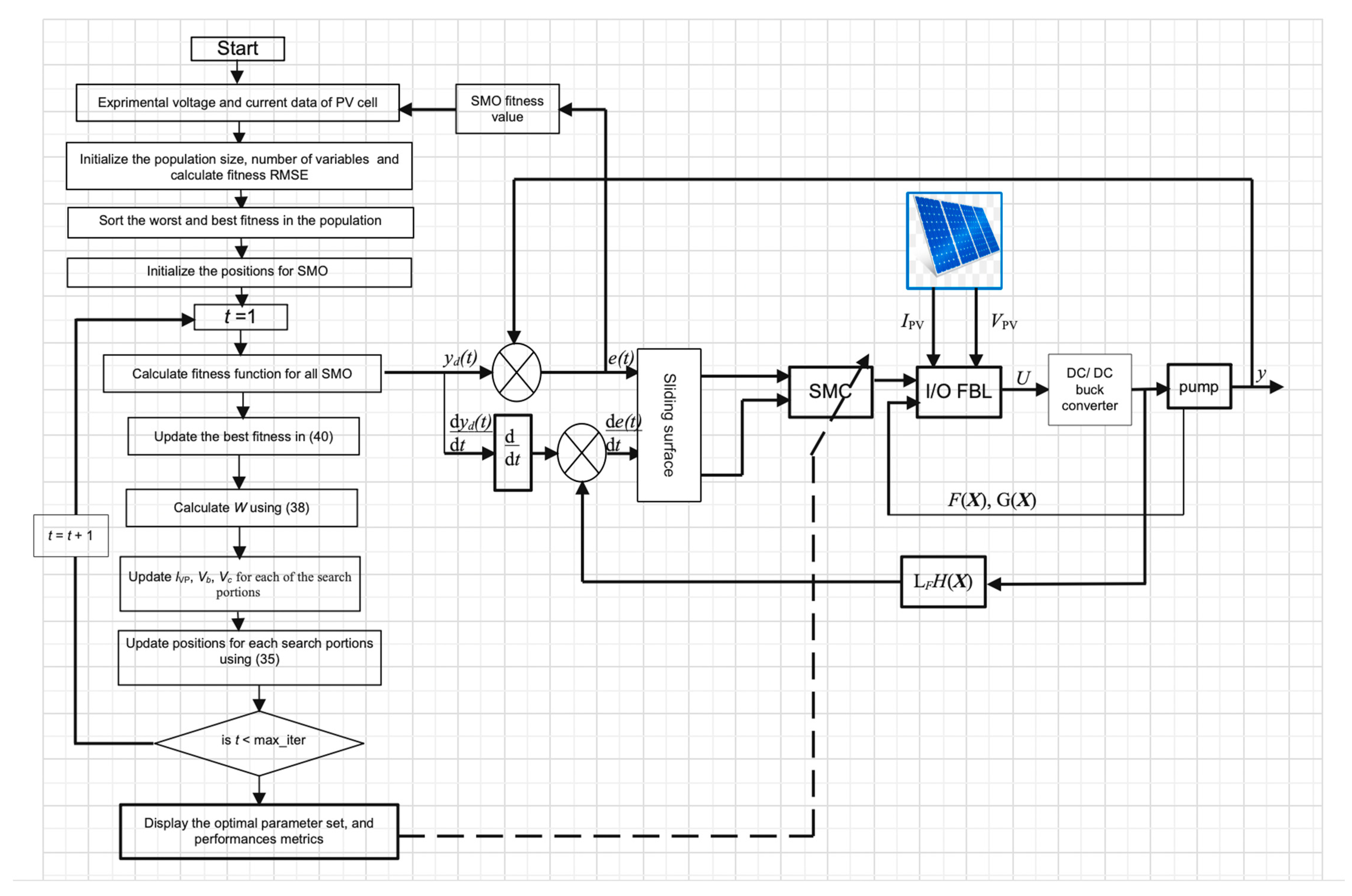
4. Control Design Based on the Slime Mould Algorithm

4.1. Introduction to the Slime Mould Algorithm and Problem Expression

Here, we recommend the application of the SMO stochastic technique to ascertain the PV system’s controller gains. An explanation is also provided on how the values of the solution vector variables are adjusted for the SMO application to the root mean square error (RMSE) [40,41,42,43,44,45,46,47,48,49,50,51,52].
For this investigation, the assumptions of the PV system’s parameter values are depicted in Table 1. As made obvious in the expression stated in (5), nonlinear functions manage the PV system as a function of the system state variables [ I A ,   Ω ,   I L ,   V A ] . Mostly, the solution to these types of systems involves the usage of analytical, numerical, or metaheuristic procedures. The stochastic SMO approach offers exceptional arithmetical modeling of the optimization problem through the utilization of adaptive weights, which is a replication of the procedure for obtaining both positive and negative feedbacks in the propagated wave. The authenticity of PV cell’s parameters, extracted by means of a theoretical model, is assessed by the RMSE between the measured experimental and simulated outputs. The RMSE can be utilized to represent the overall difference between every measured and approximated pair through an expression given by
RMSE = 1 q i = 1 q f ( parameter ) 2 ,
where q is the sample size or the number of experimental data. For the recommended approach, the minimum RMSE according to (34) is considered. The implementation of the SMO technique to approximate the parameters of the model is based on a regulation that is representative of the solution vector in all iterations.

4.2. Fundamentals of the Concept

Developed and introduced in [44], the SMO is a population-centered metaheuristic optimization algorithm originating from the unique natural oscillatory conduct of slime mould. The algorithm is based on the search for the optimal route, towards a solution to the complex optimization problems, using a merger of positive and negative feedbacks, much like the approach of slime mould during the pursuit of food. The mould adjusts its food search maneuvers, based on the quality of the food, in an exceedingly vigorous fashion. The mould is also equipped with the capability to craft a structure resembling an arrangement of veins, which simultaneously links a variety of food sources.
A mathematical imitation of the slime mould behavior, regarding the contraction mode, is stated as [44]
Γ ( i + 1 ) = { Γ b ( i + 1 ) + V b ( W   Γ a ( i ) Γ b ( i ) ) ,   s < l , V c       Γ ( i ) ,   s l ,
where Γ is the slime mould position; V b is a parameter equal to [ c , c ] , with V c linearly decreasing from 1 to 0; Γ b is the individual location with the greatest currently detected aroma concentration; W is the slime mould weight; Γ a and Γ b represent a pair of individuals chosen from the swarm, in an arbitrary mode; and i denotes the current iteration. The variable l defined in (35) is the dynamically altered probability index given as
l = tanh | O ( i ) L F | ,   i { 1 , , n } ,
where O ( i ) signifies the fitness of Γ and L F is the finest (optimal) fitness identified in the prevailing iterative process. Note that V b given in (35) is stated as V b = [ c , c ] , with
c = tanh 1 ( 1 1 / max _ iter ) ,
where max _ iter is the maximum iteration. The slime mould weight is formulated as
W ( smell   index ( i ) ) = { 1 + s   log ( L F s L F W F + 1 ) ,   condition ; 1 s   log ( L F O ( i ) L F W F + 1 ) ,   others ;
where smell   index ( i ) = sort ( O ( i ) ) , that is, the series of fitness values classified (which rises in the minimum value problem); “condition” indicates that O ( i ) is ranked among the first half of the population; s is a random value in the interval [0, 1]; and W F is the least fitness value attained during the prevailing iterative process. The mathematical formula for revising the slime mould position is obtained as
Γ * = { rand ( u b l b ) + l b ,   rand < s ; Γ b ( i + 1 ) + V b ( W   Γ a ( i ) Γ b ( i ) ) ,   s < l ; V c   Γ ( i ) ,   s l ;
where l b and u b are the lower and upper bounds, respectively, and s and “ rand ” denote the random value in the range 0 to 1. The key maneuver that needs to be implemented for an SMO algorithm is the fitness function. The assessment exercise concludes with the determination of the error between y d ( t ) and y ( t ) , as expressed by
P ( t ) = 0 ( y d ( t ) y ( t ) ) 2 d t = 0 e ( t ) 2 d t .

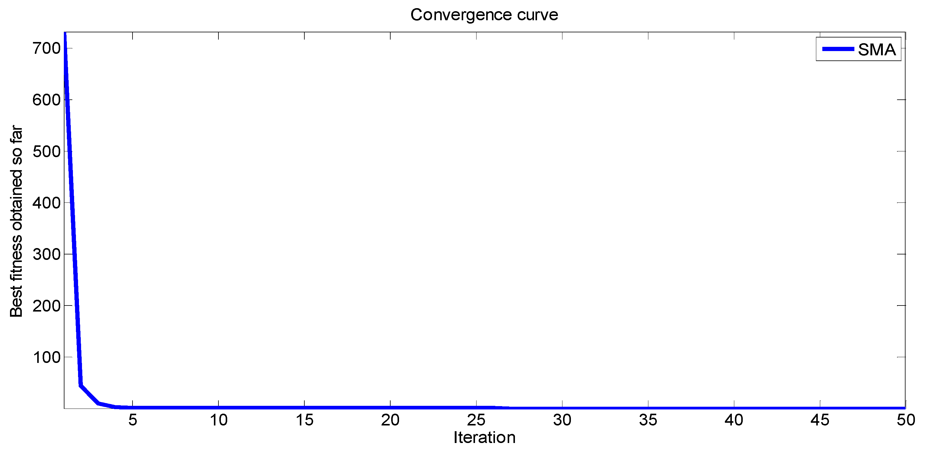
4.3. Algorithm Synthesis

Algorithm 1 summarizes the SMO control strategy as it was designed.
Algorithm 1 SMO control strategy
Step 1: Activate the PV system’s initial population as X ( 0 ) = [ I A ( 0 ) ,   Ω ( 0 ) ,   I L ( 0 ) ,   V A ( 0 ) ] T .
Step 2: Fix the boundaries for all parameters.
Step 3: Establish the fitness function expressed through P = 0 e ( t ) 2 d t .
Step 4: Set the parameter population size of the SMO method and max _ iter .
Step 5: Fix the locations for the slime mould Γ i , for i   { 1 , , n } , as l max _ iter :
  5.1 Compute the fitness function for all the slime mould.
  5.2 Ascertain the function T (X,D) depicted by (7).
  5.3 Calculate the control law expressed by (24).
  5.4 Re-assess for the finest fitness P best = min { 0 e ( t ) 2 d t } .
  5.5 State the weight W by way of (36).
  5.6 Re-evaluate l ,   V b ,   V c for the search portions.
  5.7 Re-detect positions for each of the search portions through (37).
  5.8 Do i = i + 1 .
Step 6: Resume P best = min { 0 e ( t ) 2 d t } .
Step 7: Confirm the control U formulated in (31).

4.4. SMO Control Implementation and Simulation Breakdown

The SMO application to the PV cell variable determination for the models entails the lowering of the RMSE value to its minimum. After each iteration, the cost function is altered for the experimental value from the inductor-voltage characteristic, which requires minimization to acquire the parameters. The efficiency and quickness of the optimization process for ascertaining the parameters of the PV system are determined by the algorithm’s fitness function. The use of the SMO algorithm to vary the fitness function during parameter estimation is depicted in Figure 9. To arrive at the cost function objective, the solution is updated over the iteration. Figure 10 displays the SMO flowchart for the parameter determination and control strategy. The controlled PV system simulation was conducted in a Matlab environment. Table 2 lists the numerical parameter values used. With the SMO technique, the varying gains are regarded as fundamental elements, affecting the algorithm convergence behavior. Table 3 provides the used parameters and settings of the SMO algorithm.
The effectiveness of the stabilizing control design and the vibrant performance of the DC converter are made evident in Figure 11, Figure 12, Figure 13 and Figure 14. Despite the arbitrary environmental disturbances and their unwelcome impact on the system, the supply delivered by the pump is well filtered and comes with high accuracy. To assess effectiveness of the SMO controller, we compare it with several conventional approaches.
Figure 11, Figure 12, Figure 13 and Figure 14 show the superiority of the SMO system in terms of reducing disturbance and chattering, as well as curbing the occurrence of unwanted dynamical behavior. As noted from Figure 15, the unwanted chattering feature was relatively subdued. This is attributed to the combination comprising the SMO module and SMC-based FBL, in which controller gain tuning is carried out unceasingly. The designed procedure has the capacity to surmount the uncertainty problem brought about arbitrary external disturbances to the PV system.
Table 4 illustrates the accuracy of the SMO controller for the advanced K 1 gain tuning stated in (33) and the corresponding control effort. In this table, such past aspects are compared against the conventional I/O FBL control defined in (5), the decoupling I/O FBL established in (24), and the analytical SOSM control as given under the analytical form presented in (33). The SMO technique offers the lowest control effort with its selected accurate controller gain, which confirms the efficiency of the designed technique.
Table 5 confirms the same conclusion regarding the efficiency and superiority of the developed schemes. Indeed, the best accuracy for the RMSE values among the simulation slots is obtained for the SMO method. For tracking control purposes, we conclude that the designed algorithm is efficient in the case of the PV system. Indeed, the dynamics of such a process is relatively slow compared to the required algorithm convergence time.

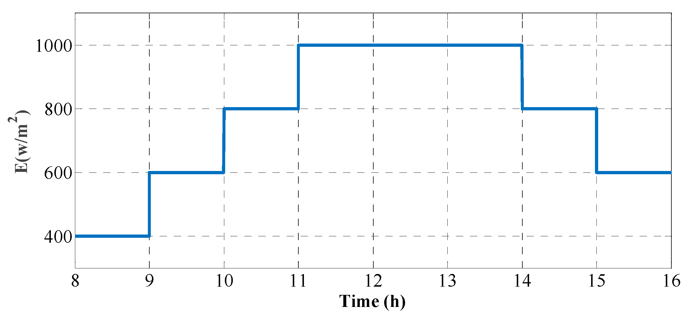
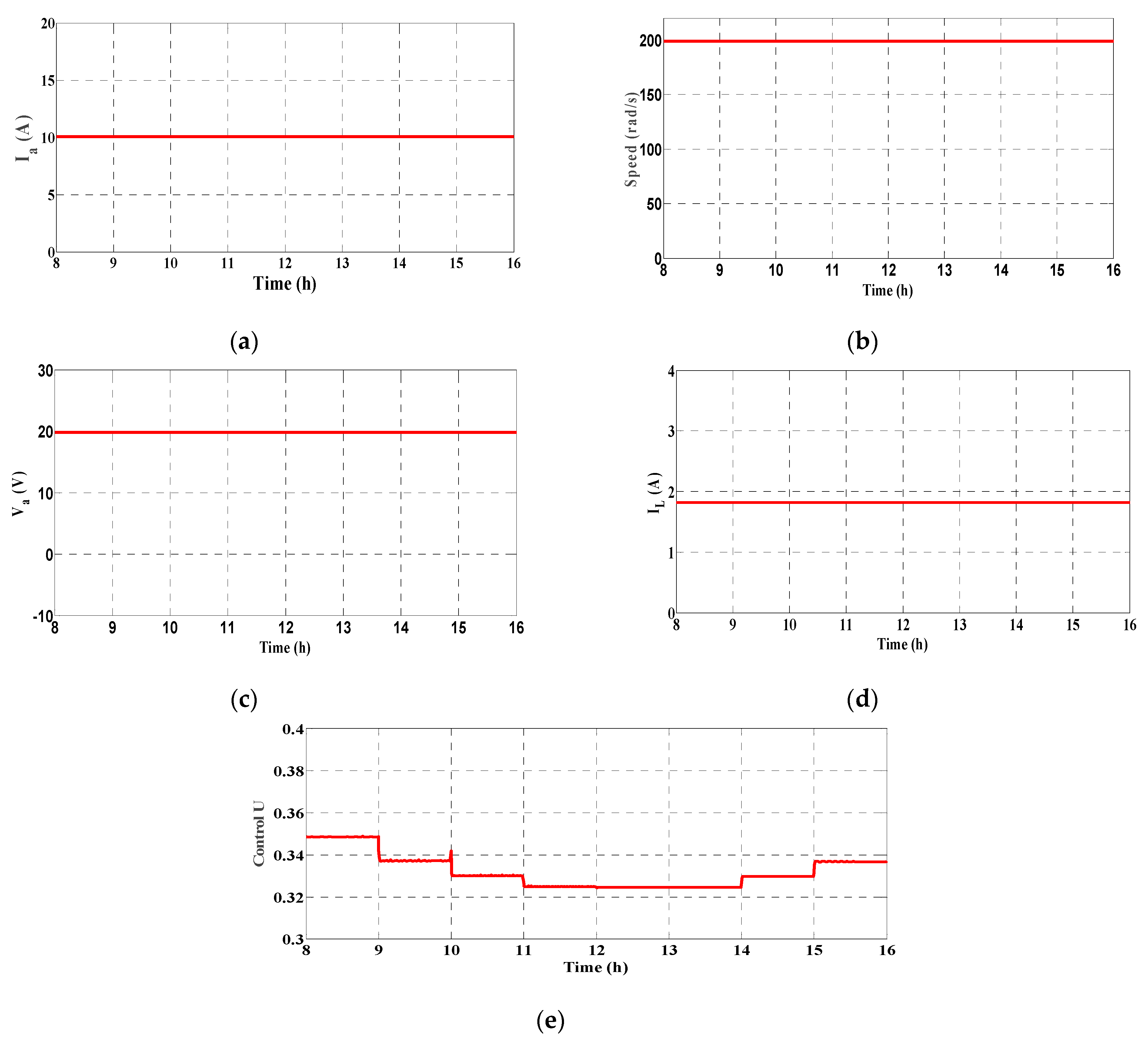
4.5. New Scenario under Natural Irradiance

We ran the entire simulation study by considering a new scenario for the natural irradiance around the value of 1000 W/m2. The experimental results are reported next:
(i)
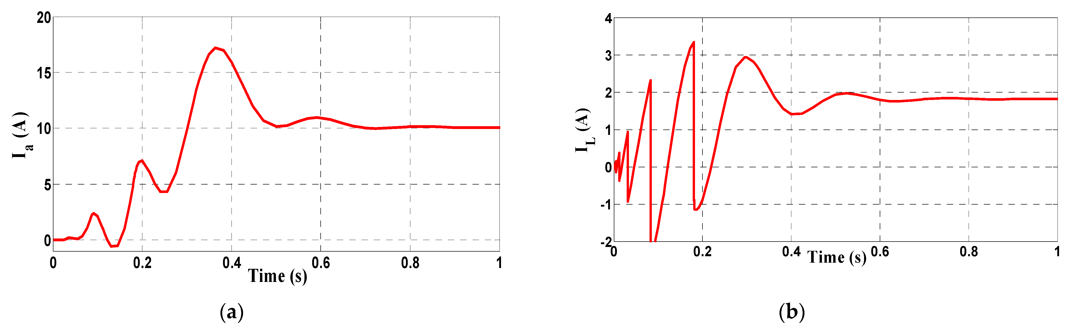
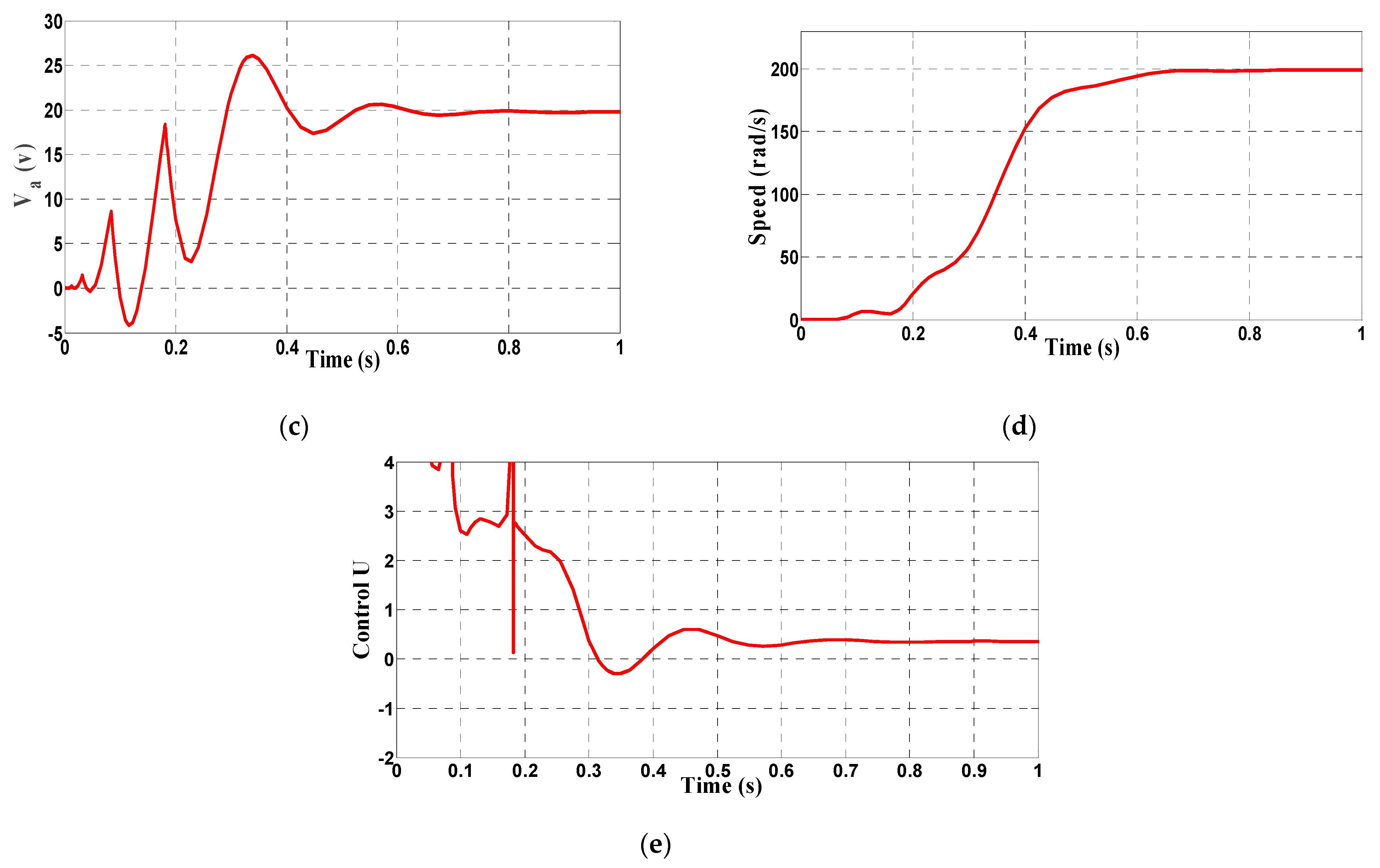
We state clearly that our designed scheme offers satisfactory performance as can be seen in Figure 16.
(ii)
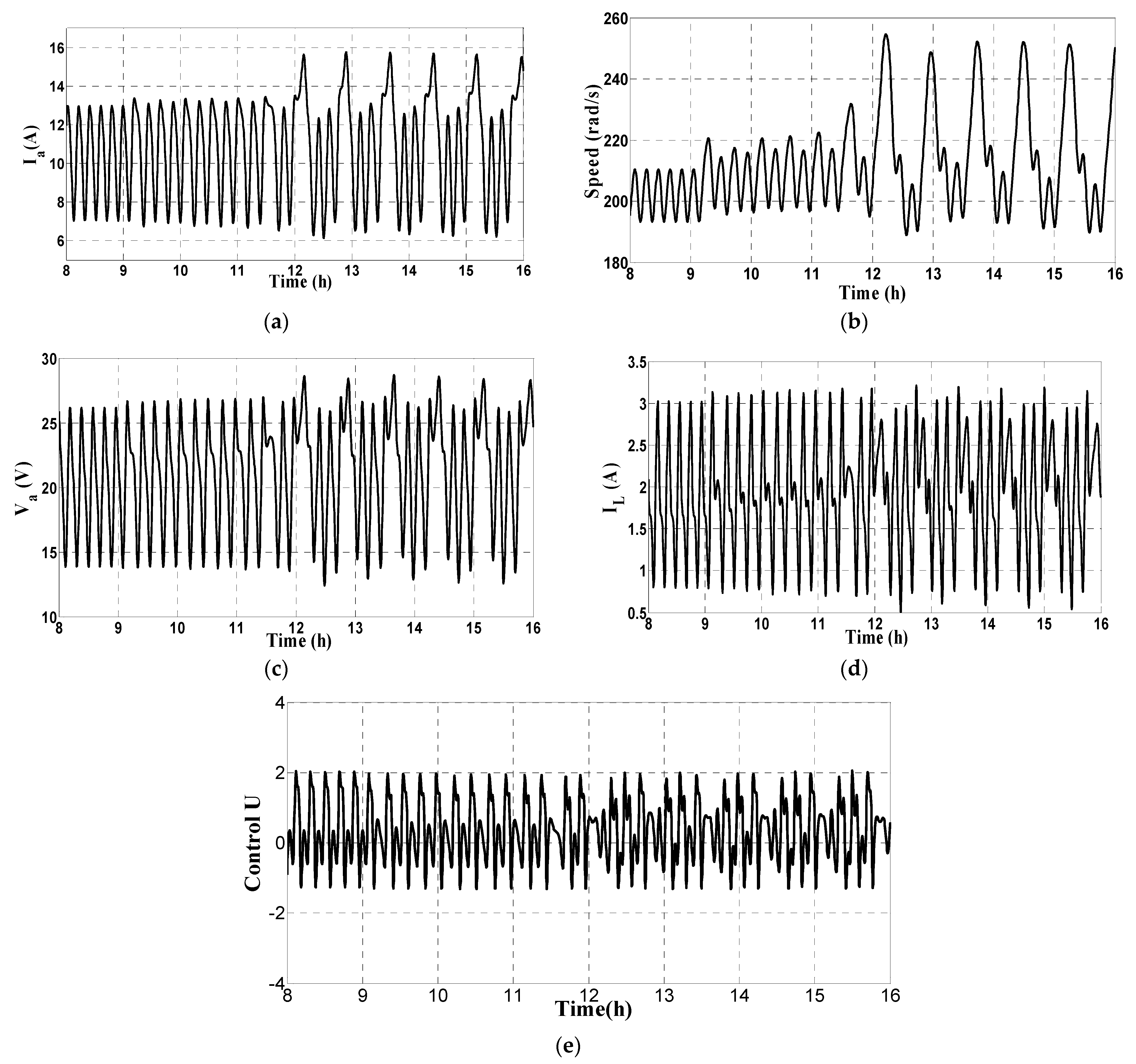
The first study is performed by using the fundamental FBL technique without applying disturbing signals to the closed-loop system. This fact is shown in Figure 17. Notice that FBL provides high performance in stabilizing the controlled system.
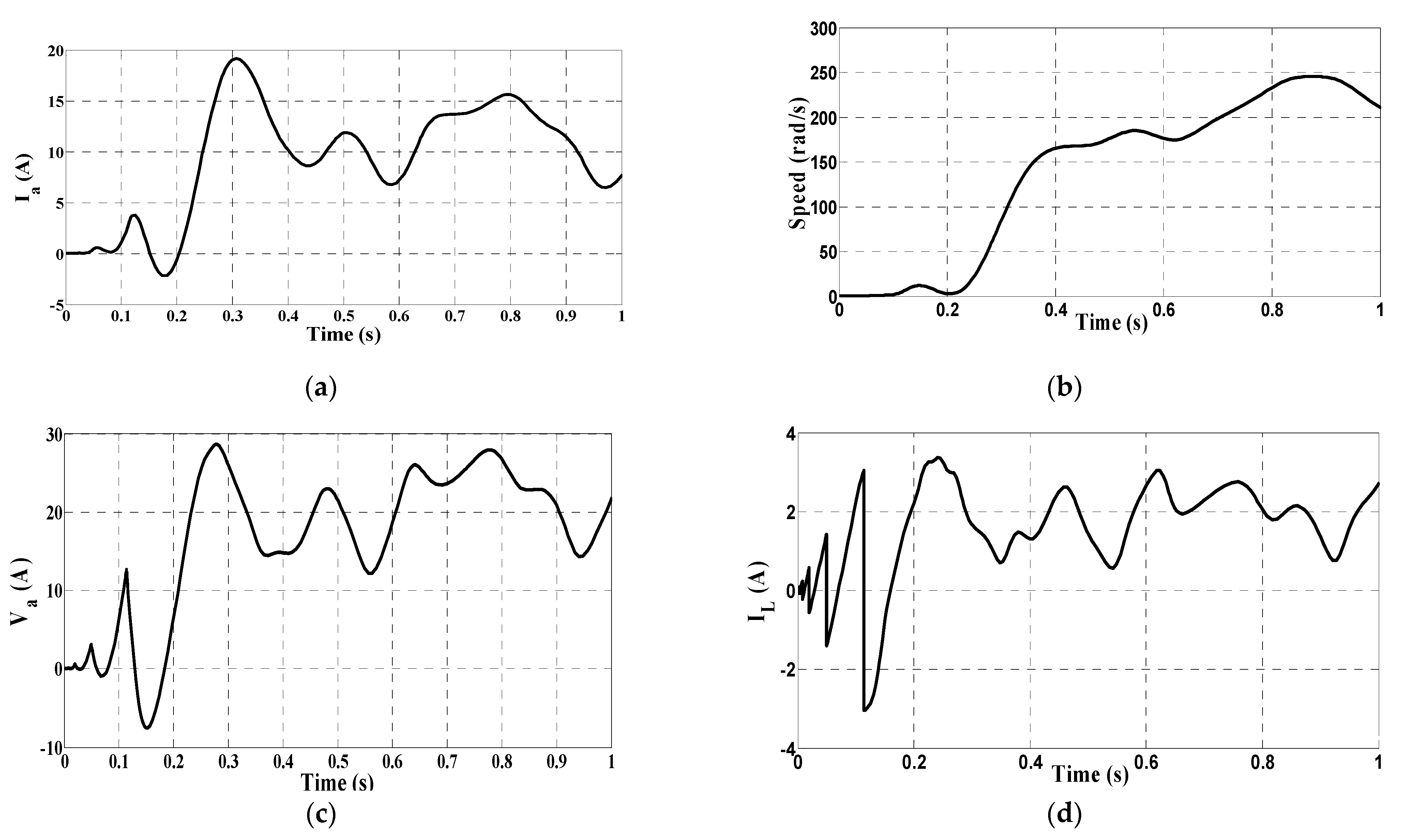
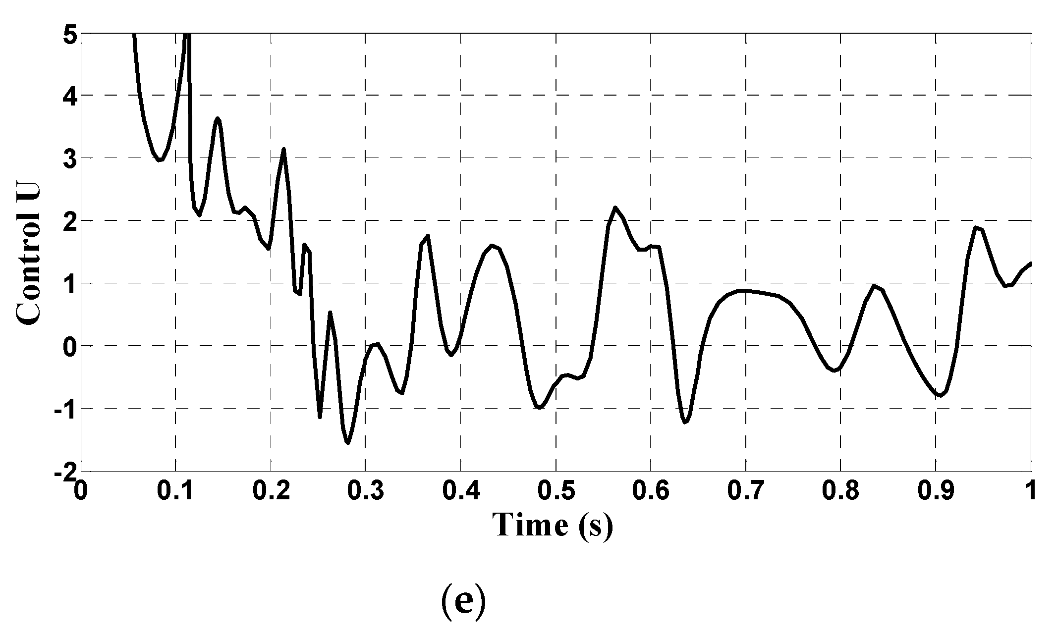
(iii)
The second study is conducted by considering disturbed random and matched signals, as shown in Figure 18. Note that the dynamical performance is highly affected.
(iv)
Observe that, in this new scenario, as expected, the FBL controller totally loses its dynamical performance.
(v)
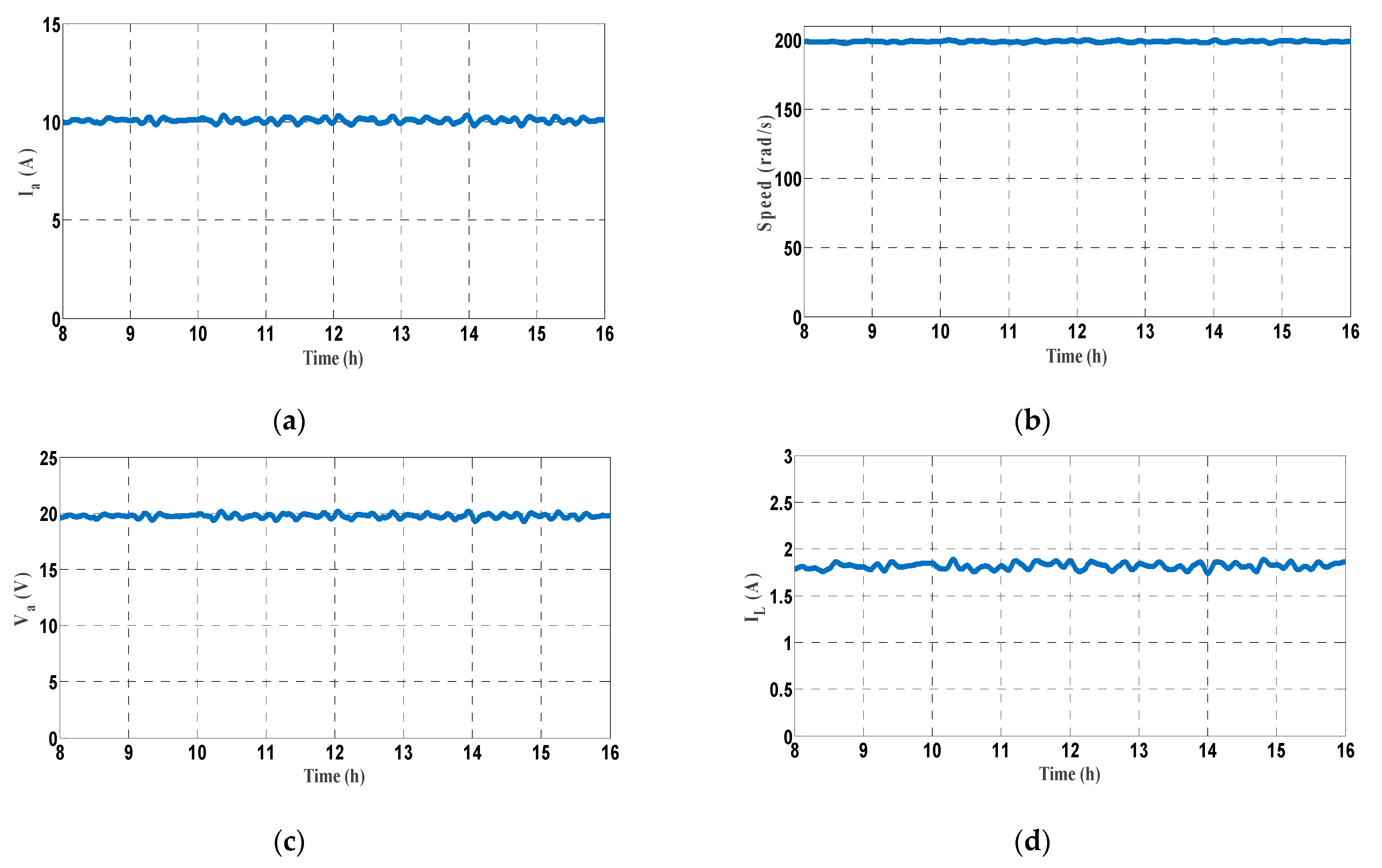
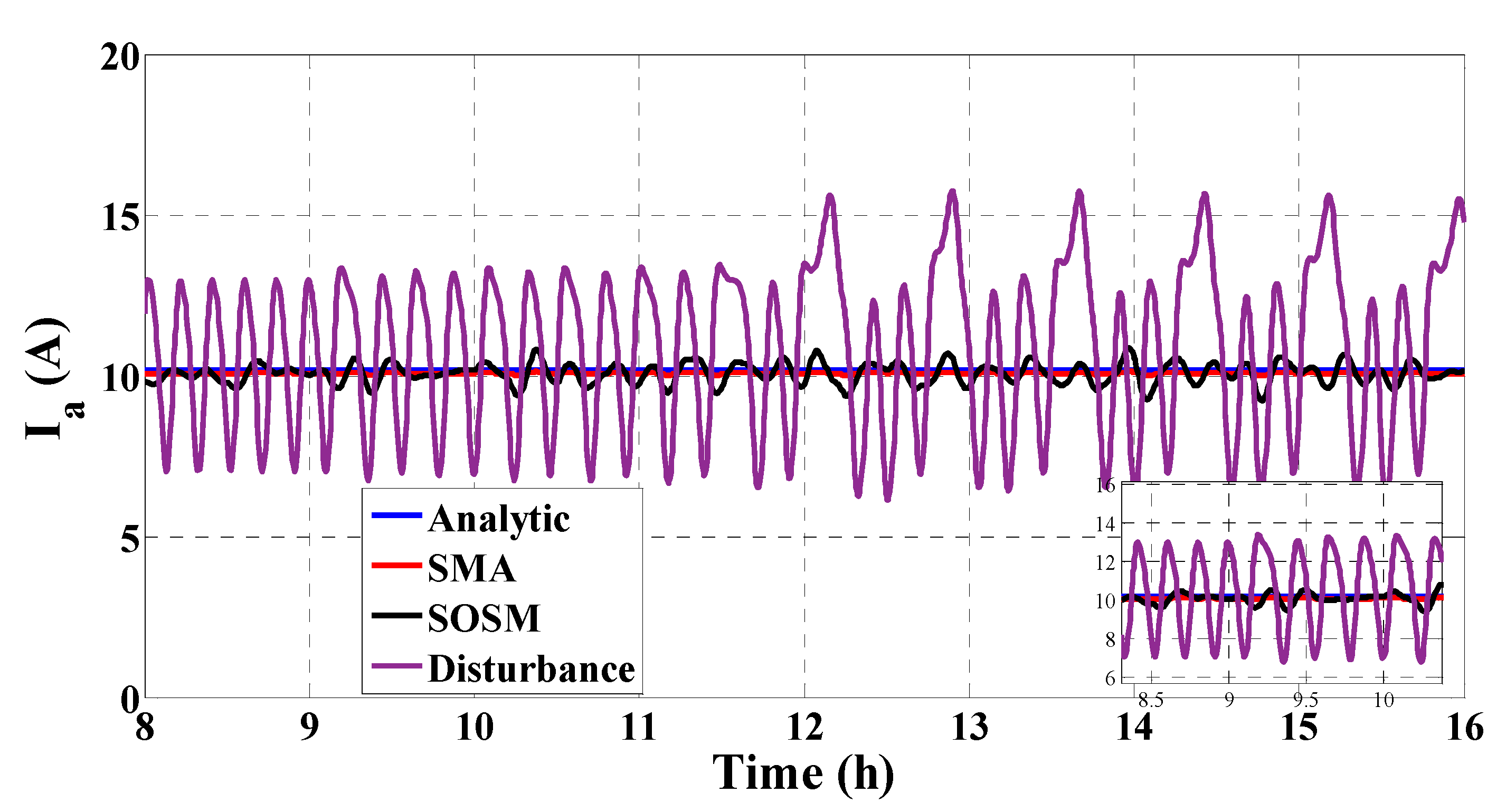
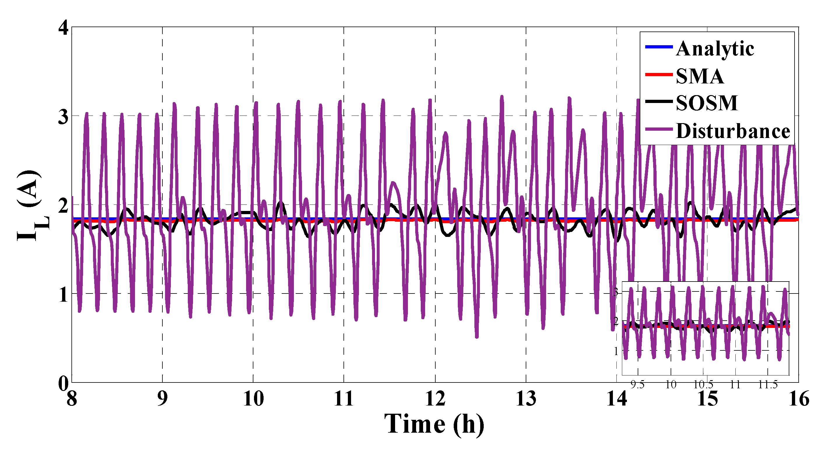
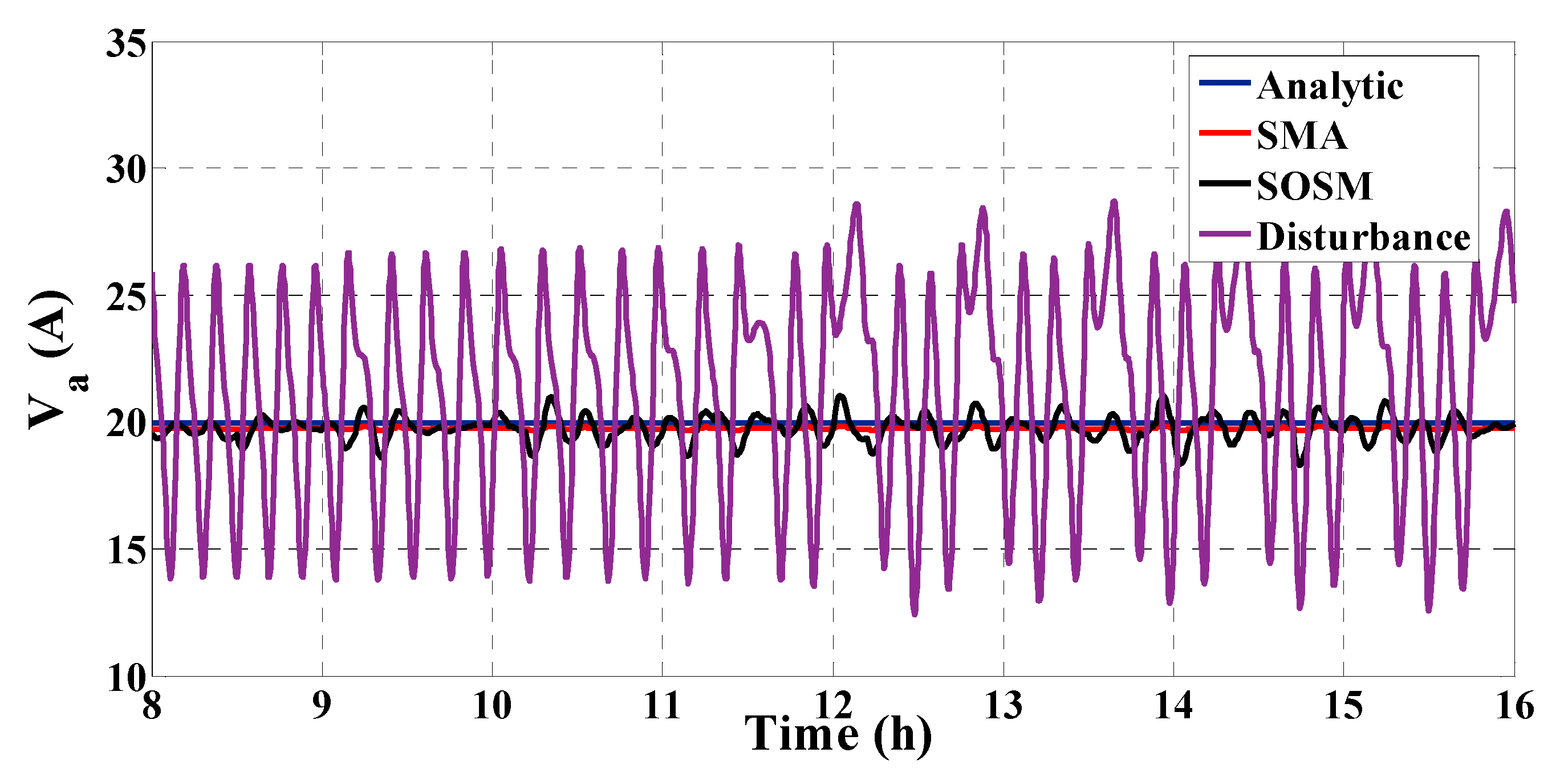
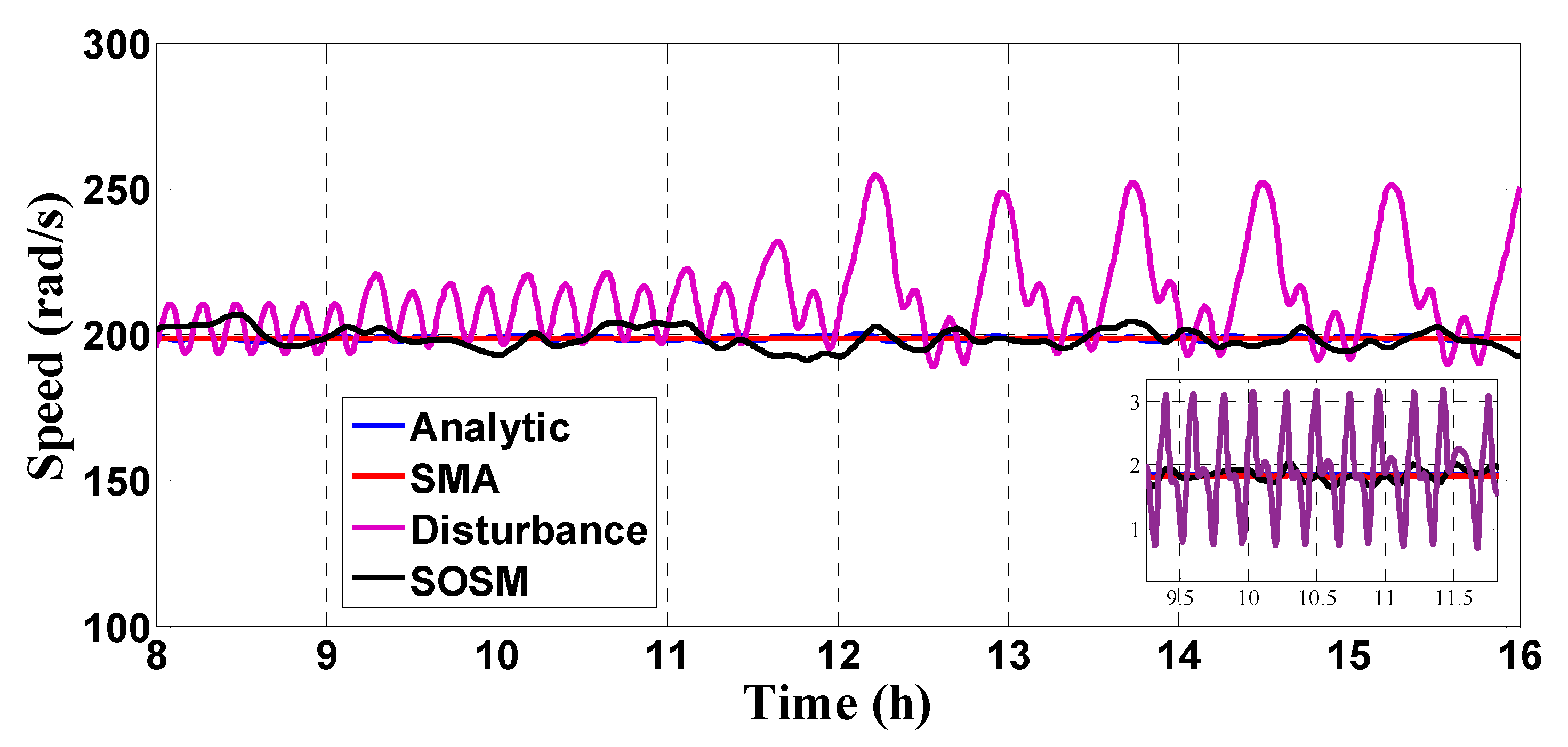
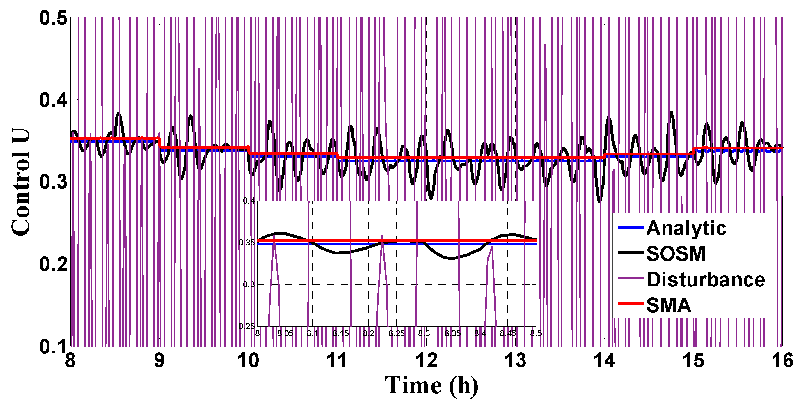
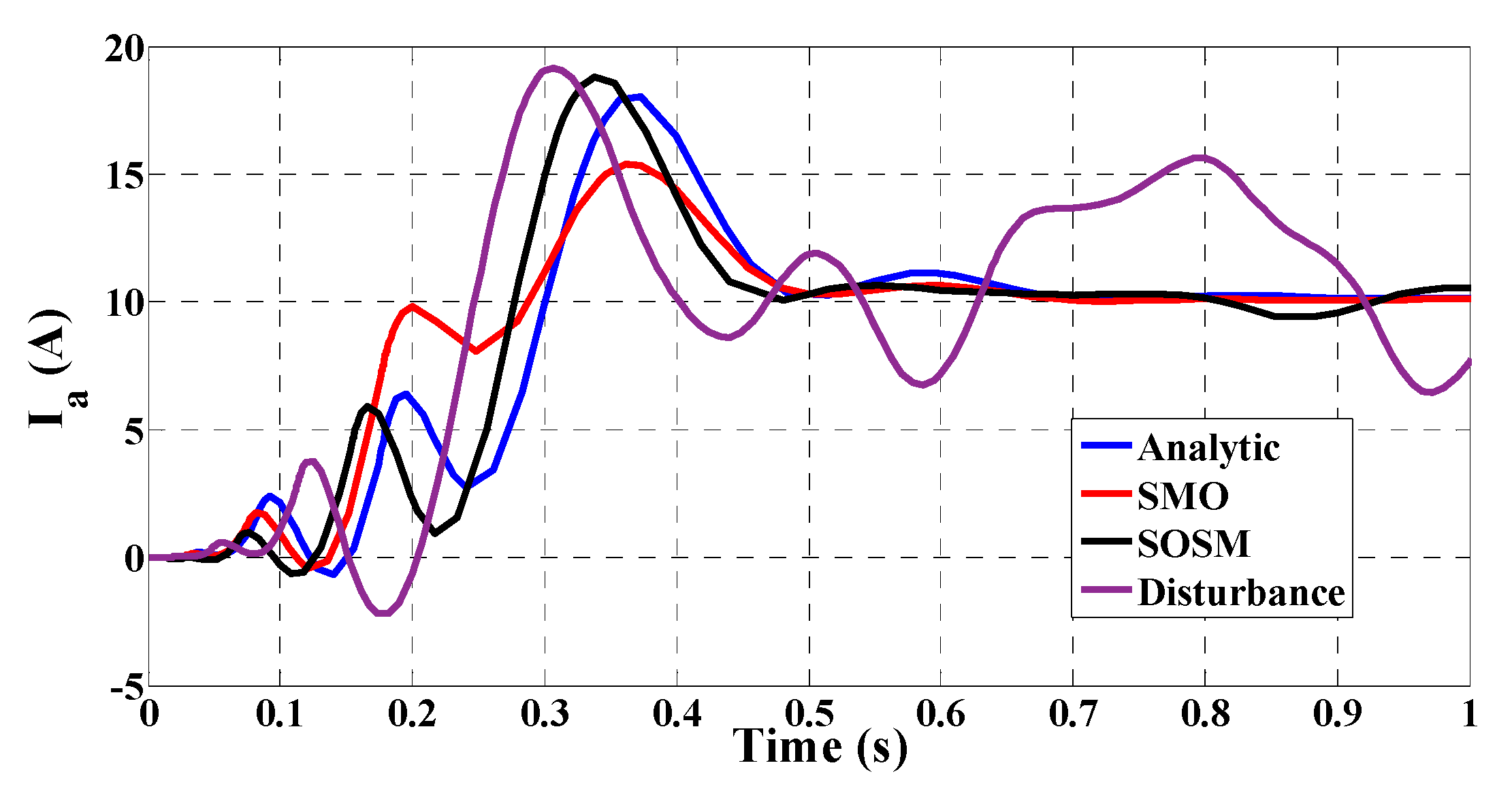
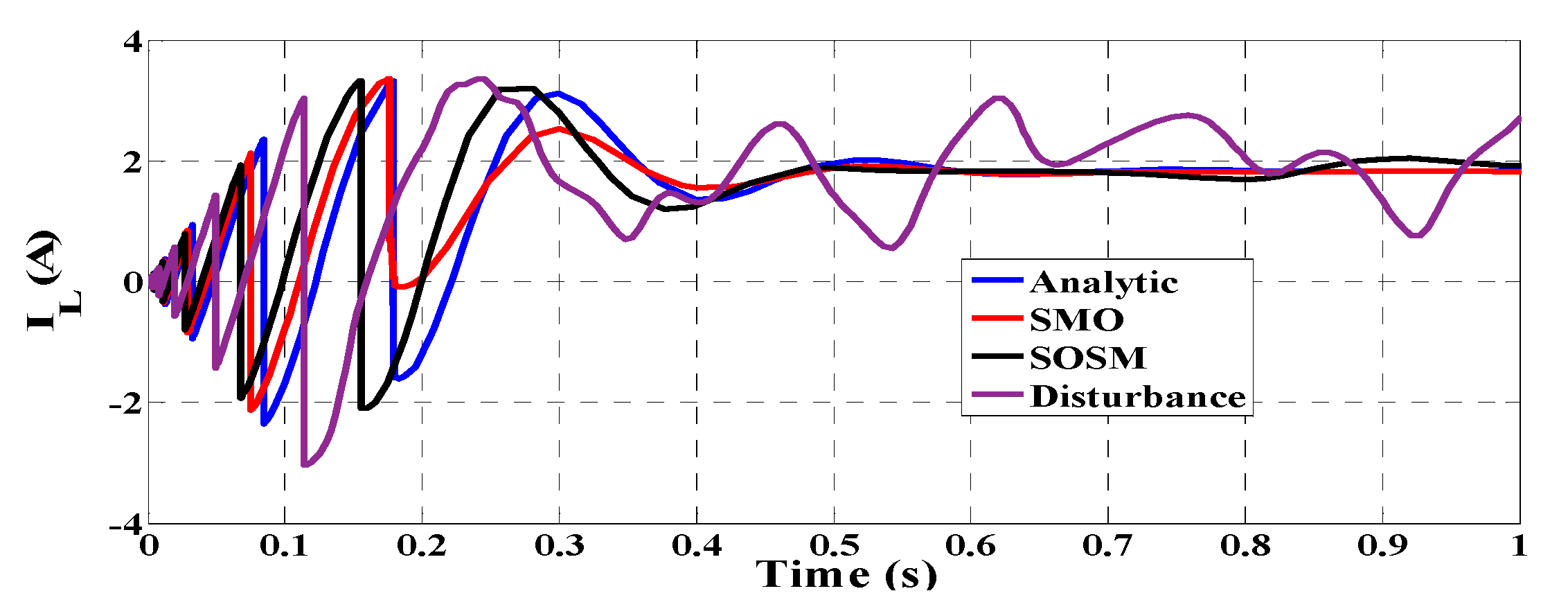
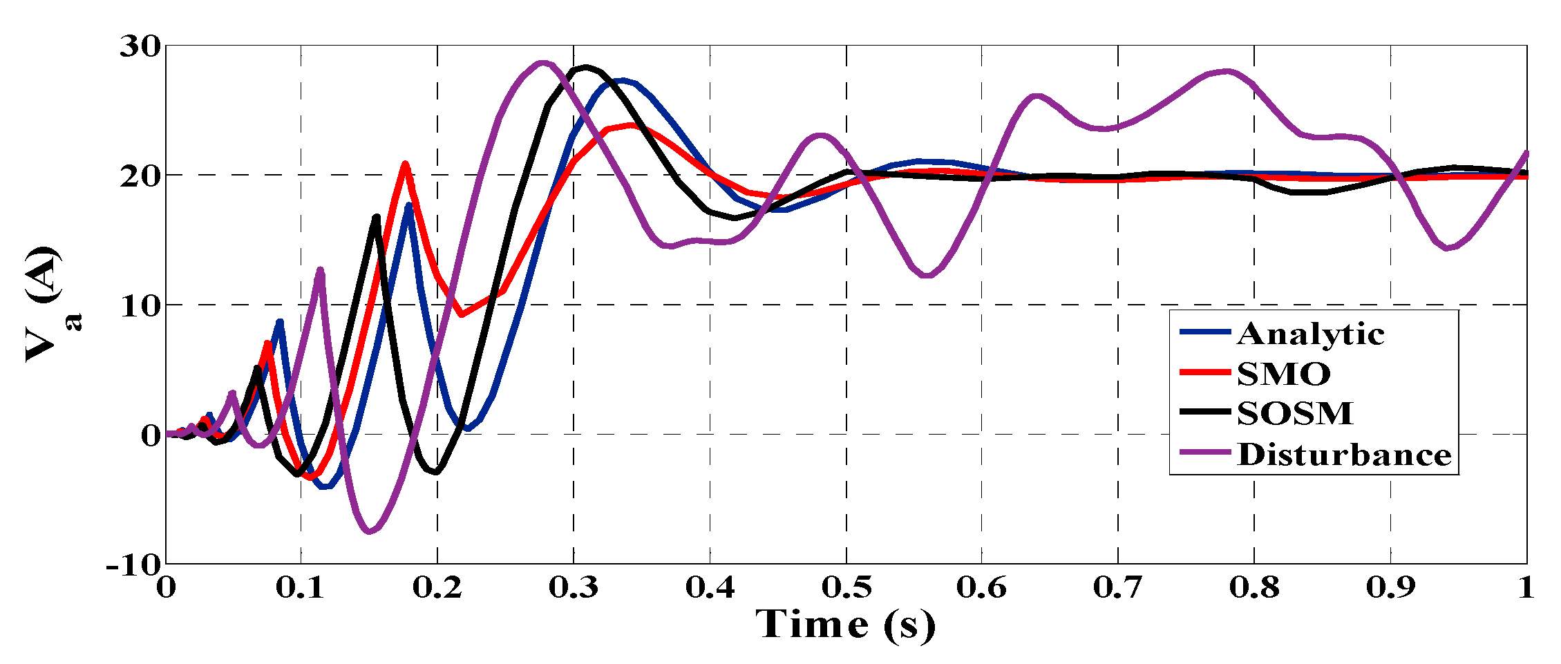
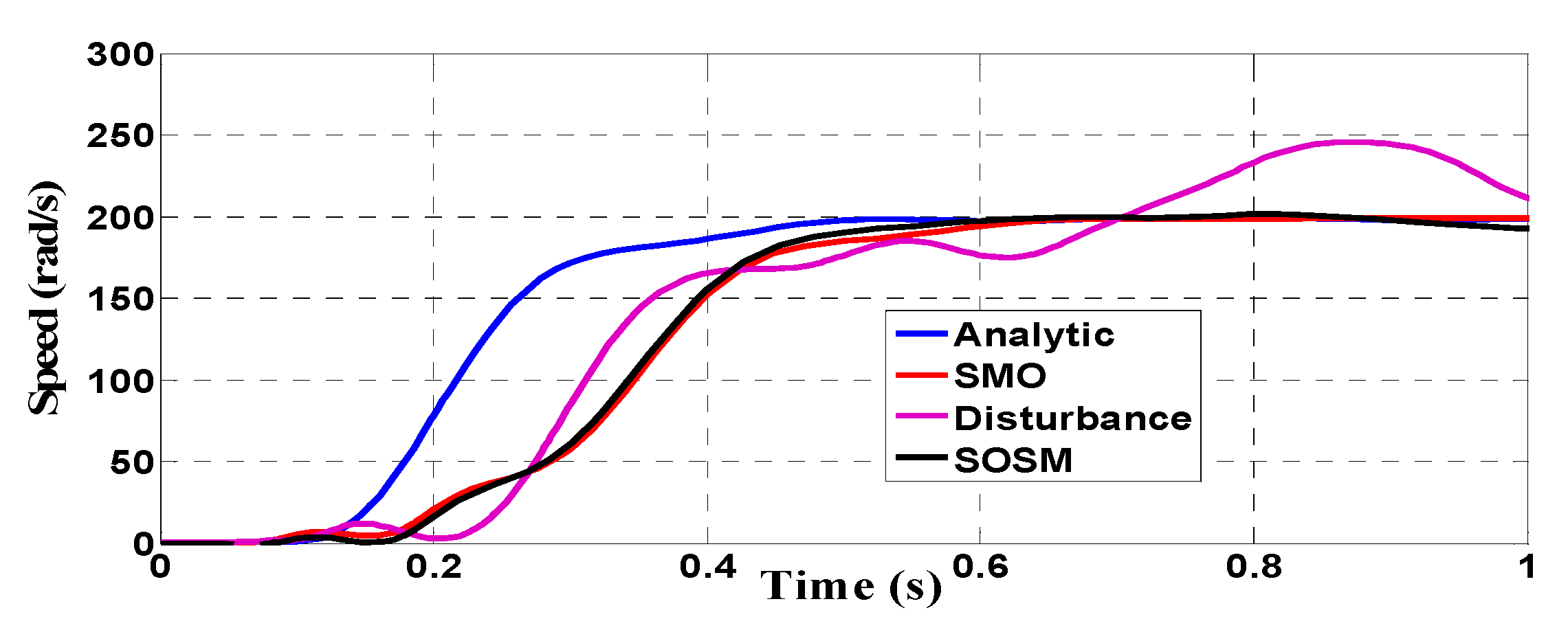
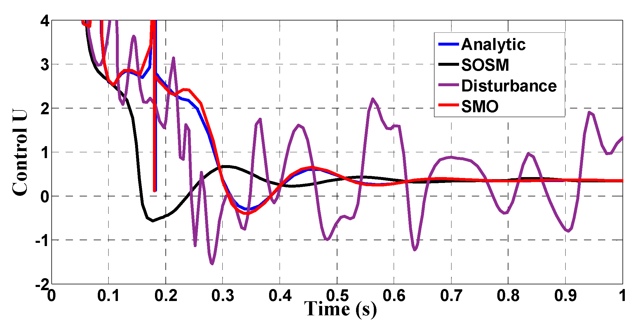
The designed SMO-SMC-FBL scheme developed in this paper is now compared to fundamental FBL (analytic technique ignoring disturbances), SOSM (analytic second-order sliding mode considering disturbance), and FBL (analytic technique considering disturbances). The results are shown in Figure 19, Figure 20, Figure 21, Figure 22 and Figure 23, from where we detect that the superiority of the SMO technique is obvious. Indeed, the global behavior of the controlled system is stable and accurate.
(vi)
Therefore, the steady-state regime is attained in a quite satisfactory way.

5. Conclusions

In this paper, we have proposed an advanced metaheuristic approach that involved second-order sliding mode control in association with feedback linearization. This approach solves control problems related to unspecified state disturbances and parametric uncertainties plaguing the photovoltaic system. The simulation conducted here verified that the input–output feedback linearization fails to ensure a problem-free decoupling of the desired output variable from unmeasured disturbances. Precise determination of the unmeasured states is needed to define the control law ensuring full decoupling. This leads to the recommended incorporation of the feedback linearization method for decoupling the output from disturbance and of a sliding mode control technique for ensuring the robustness of the controller. In addition, this combination has reduced the influence of external disturbances, accelerating the dynamic response to parameter and process modeling uncertainties.
An optimization algorithm was implemented to enhance controllers of photovoltaic systems and to diminish chattering, while the slime mould facilitated adjustments to the gains of the sliding mode, which ensured the stability of the process. Therefore, the general performance of the closed-loop photovoltaic system was significantly enhanced.
Future work should include investigations on the viability of applying the recommended technique in the discrete time domain. While the control structure utilizes a real-time software tool, the consequences of sampling frequency and process delays, derived from the control input, were not precisely stated for this undertaking. Issues concerning input saturation should also be considered for any upcoming work in this area.

Author Contributions

Conceptualization, S.C., H.J., H.A. and V.L.; data curation, S.C. and H.A.; formal analysis, S.C., H.J. and V.L.; investigation, H.J. and M.K.; methodology, S.C., H.J., H.A. and V.L.; software, S.C.; validation, M.K., R.A. and V.L..; visualization, R.A., M.K., H.J. and V.L.; writing—original draft preparation, S.C., H.A., R.A., M.K. and H.J.; writing—review and editing, V.L. All authors have read and agreed to the published version of the manuscript.

Funding

This research was funded by the Research Deanship of Hail University, KSA (Project Number RG-21 127).

Institutional Review Board Statement

Not applicable.

Informed Consent Statement

Not applicable.

Data Availability Statement

Data are available upon request.

Acknowledgments

The authors acknowledge the Research Deanship of Hail University, KSA, for the administrative, financial, and technical support. The authors also thank the Editors and three Reviewers for their constructive comments, which helped to obtain an improved version of the paper.

Conflicts of Interest

The authors declare no conflict of interest.

References

  1. Rekioua, D.; Matagne, E. Optimization of Photovoltaic Power Systems: Modelization, Simulation and Control; Springer: New York, NY, USA, 2012. [Google Scholar]
  2. Alfegi, E.M.A.; Sopian, K.; Othman, M.Y.H.; Yatim, B.B. Transient mathematical model of both side single pass photovoltaic thermal air collector. ARPN J. Eng. Appl. Sci. 2007, 2, 22–26. [Google Scholar]
  3. Xie, W.T.; Dai, Y.J.; Wang, R.Z.; Sumathy, K. Concentrated solar energy applications using Fresnel lenses: A review. Renew. Sustain. Energy Rev. 2011, 15, 2588–2606. [Google Scholar] [CrossRef]
  4. Mokarram, M.; Mokarram, M.J.; Khosravi, M.R.; Saber, A.; Rahideh, A. Determination of the optimal location for constructing solar photovoltaic farms based on multi-criteria decision system and Dempster–Shafer theory. Sci. Rep. 2020, 10, 8200. [Google Scholar] [CrossRef] [PubMed]
  5. Fialho, L.; Melício, V.; Mendes, M.D.; Estanqueiro, A.; Collares-Pereira, M. PV systems linked to the grid: Parameter identification with a heuristic procedure. Sust. Energy Technol. Assess. 2015, 10, 29–39. [Google Scholar] [CrossRef] [Green Version]
  6. Mohamed, N.; Aymen, F.; Ali, Z.M.; Zobaa, A.F.; Aleem, S.H.E.A. Efficient power management strategy of electric vehicles-based hybrid renewable energy. Sustainability 2021, 13, 7351. [Google Scholar] [CrossRef]
  7. Kim, K.; McKay, R.B.; Hoai, N.X. Recursion-based biases in stochastic grammar model genetic programming. IEEE Trans. Evol. Comp. 2016, 20, 81–95. [Google Scholar] [CrossRef]
  8. Chaouch, H.; Charfeddine, S.; Aoun, S.B.; Jerbi, H.; Leiva, V. Multiscale monitoring using machine learning methods: New methodology and an industrial application to a photovoltaic system. Mathematics 2022, 10, 890. [Google Scholar] [CrossRef]
  9. Liu, C.; Luo, Y.; Huang, J.; Liu, Y. A PSO-based MPPT algorithm for photovoltaic systems subject to inhomogeneous insolation. In Proceedings of the 6th International Conference on Soft Computing and Intelligent Systems, and the 13th International Symposium on Advanced Intelligence Systems, Kobe, Japan, 20–24 November 2012; pp. 721–726. [Google Scholar]
  10. Miyatake, M.; Veerachary, M.; Toriumi, F.; Fujii, N.; Ko, H. Maximum power point tracking of multiple photovoltaic arrays: A PSO approach. IEEE Trans. Aerosp. Electron. Syst. 2011, 47, 367–380. [Google Scholar] [CrossRef]
  11. Fernhndez, B.; Hedrick, K. Control of multivariable nonlinear systems by the sliding mode method. Int. J. Control 1987, 46, 1019–1040. [Google Scholar] [CrossRef]
  12. Sira-Ramirez, H. Sliding regimes in general nonlinear systems: A relative degree approach. Int. J. Control 1989, 50, 1487–1506. [Google Scholar] [CrossRef]
  13. Elmali, H.; Olga, N. Robust output tracking control of nonlinear MIMO systems via sliding mode technique. Automatica 1992, 45, 145–151. [Google Scholar] [CrossRef]
  14. Chiacchiarini, H.; Desages, A.C.; Romagnoli, J.A.; Palazoglu, A. Variable structure control with a second-order sliding condition: Application to a steam generator. Automatica 1995, 31, 1157–1168. [Google Scholar] [CrossRef]
  15. Charfeddine, S.; Boudjemline, A.; ben Aoun, S.; Jerbi, H.; Kchaou, M.; Alshammari, O.; Elleuch, Z.; Abbassi, R. Design of a fuzzy optimization control optimization control structure for nonlinear systems: A disturbance-rejection method. Appl. Sci. 2021, 11, 2612. [Google Scholar] [CrossRef]
  16. Han, S.H.; Tran, M.S.; Tran, D.T. Adaptative sliding mode control for a robotic manipulator with unknown friction and unknown control direction. Appl. Sci. 2021, 11, 3919. [Google Scholar] [CrossRef]
  17. Yen, V.T.; Nan, W.Y.; Van Cuong, P. Robust adaptive sliding mode neural networks control for industrial robot manipulators. Int. J. Control Autom. Syst. 2019, 17, 783–792. [Google Scholar] [CrossRef]
  18. Askarzadeh, A.; Dos Santos Coelho, L. Determination of photovoltaic modules parameters at different operating conditions using a novel bird mating optimizer approach. Energy Conv. Manag. 2015, 89, 608–614. [Google Scholar] [CrossRef]
  19. Utkin, V.; Guldner, J.; Shi, J. Sliding Mode Control in Electro-Mechanical Systems; CRC Press: Boca Raton, FL, USA, 2009. [Google Scholar]
  20. Perruquetti, W.; Barbot, J.P. Sliding Mode Control in Engineering; CRC Press: Boca Raton, FL, USA, 2002. [Google Scholar]
  21. Roopaei, M.; Jahromi, M.Z. Chattering-free fuzzy sliding mode control in MIMO uncertain systems. Nonlin. Anal. Theory Meth. Appl. 2009, 71, 4430–4437. [Google Scholar] [CrossRef]
  22. Amer, A.F.; Sallam, E.A.; Elawady, W.M. Adaptive fuzzy sliding mode control using supervisory fuzzy control for 3 DOF planar robot manipulators. Appl. Soft Comput. 2011, 11, 4943–4953. [Google Scholar] [CrossRef]
  23. Jung, S. Improvement of tracking control of a sliding mode controller for robot manipulators by a neural network. Int. J. Control. Autom. Syst. 2018, 16, 937–943. [Google Scholar] [CrossRef]
  24. Lv, Z.; Qiao, L.; Cai, K.; Wang, Q. Big data analysis technology for electric vehicle networks in smart Cities. IEEE Trans. Intell. Transp. Syst. 2021, 22, 1807–1816. [Google Scholar] [CrossRef]
  25. Dizqah, A.M.; Maheri, A.; Busawon, K. An accurate method for the PV model identification based on a genetic algorithm and the interior-point method. Renew. Energy 2014, 72, 212–222. [Google Scholar] [CrossRef] [Green Version]
  26. Le, Q.D.; Kang, H.J. Finite-time fault-tolerant control for a robot manipulator based on synchronous terminal sliding mode control. Appl. Sci. 2020, 10, 2998. [Google Scholar] [CrossRef]
  27. Lee, J.; Chang, P.H.; Jin, M. Adaptive integral sliding mode control with time-delay estimation for robot manipulators. IEEE Trans. Ind. Electron. 2017, 64, 6796–6804. [Google Scholar] [CrossRef]
  28. Charfeddine, S.; Jerbi, H. Trajectory tracking and disturbance rejection for nonlinear periodic process: A gains scheduling design. Iremos 2012, 5, 1075–1083. [Google Scholar]
  29. Charfeddine, S.; Jerbi, H. A survey of nonlinear gain scheduling design control of continuous and discrete time systems. Intern. J. Model. Ident. Control 2013, 19, 203–216. [Google Scholar] [CrossRef]
  30. Charfeddine, S.; Jerbi, H.; Sbita, L. Nonlinear discrete–time gain scheduling control for affine nonlinear polynomial systems. Iremos 2013, 6, 1031–1041. [Google Scholar]
  31. Chaouech, H.; Charfeddine, S.; Ouni, K.; Jerbi, H.; Nabli, L. Intelligent supervision approach based on multilayer neural PCA and nonlinear gain scheduling. Neur. Comp. App. 2019, 31, 1153–1163. [Google Scholar] [CrossRef]
  32. Charfeddine, S.; Jerbi, H. Benchmarking of analytical and advanced nonlinear tracking approaches. J. Eng. Res. 2021, 9, 250–267. [Google Scholar] [CrossRef]
  33. Charfeddine, S.; Jerbi, H. The use of a heuristic optimization method to improve the design of a discrete-time gain scheduling control. Intern. J. Control Aut. Syst. 2021, 19, 1836–1846. [Google Scholar]
  34. Cheng, M.X.; Jiao, X.H. Observer-based adaptive l2 disturbance attenuation control of semi-active suspension with MR damper. Asian J. Control 2017, 19, 346–355. [Google Scholar] [CrossRef]
  35. Gao, F.; Wu, M.; She, J.; Cao, W. Active disturbance rejection in affine nonlinear systems based on equivalent-input disturbance approach. Asian J. Control 2017, 19, 1767–1776. [Google Scholar]
  36. Kayacan, E.; Peschel, J.M.; Chowdhary, G. A self-learning disturbance observer for nonlinear systems in feedback-error learning scheme. Eng. Appl. Artif. Intell. 2017, 62, 276–285. [Google Scholar] [CrossRef] [Green Version]
  37. Sun, T.; Zhang, J.; Pan, Y. Active disturbance rejection control of surface vessels using composite error updated extended state observer. Asian J. Control 2017, 19, 1802–1811. [Google Scholar]
  38. Andoulsi, R.; Mami, A.; Dauphin-Tanguy, G.; Annabi, M. Modelling and simulation by bond graph technique of a DC motor fed from a photovoltaic source via MPPT boost converter. Proc. CSSC 1999, 99, 4181–4187. [Google Scholar]
  39. Andoulssi, R.; Draou, A.; Jerbi, H. Nonlinear control of a photovoltaic water pumping system. Energy Proc. 2013, 42, 328–336. [Google Scholar] [CrossRef] [Green Version]
  40. Abbassi, R.; Boudjemline, A. A numerical-analytical hybrid approach for the identification of SDM solar cell unknown parameters. Eng. Technol. App. Sci. Res. 2018, 8, 2907–2913. [Google Scholar] [CrossRef]
  41. Manar, M.; Hegazy, R.; Mokhtar, A.; Emad, M.A. A new strategy based on slime mould algorithm to extract the optimal model parameters of solar PV panel. Sust. Energy Technol. Assess. 2020, 42, 100849. [Google Scholar]
  42. Yeh, W.C.; Huang, C.L.; Lin, P.; Chen, Z.; Jiang, Y.; Sun, B. Simplex simplified swarm optimization for the efficient optimization of parameter identification for solar cell models. IET Renew. Power. Gen. 2018, 51, 45. [Google Scholar] [CrossRef]
  43. Nunes, H.; Pombo, J.; Bento, P.; Mariano, S.; Calado, M. Collaborative swarm intelligence to estimate PV parameters. Energy Conv. Manag. 2019, 90, 185–866. [Google Scholar] [CrossRef]
  44. Ebrahimi, S.M.; Salahshour, E.; Malekzadeh, M.; Gordillo, F. Parameters identification of PV solar cells and modules using flexible particle swarm optimization algorithm. Energy 2019, 72, 358. [Google Scholar] [CrossRef]
  45. Li, S.; Chen, H.; Wang, M.; Heidari, A.; Mirjalili, S. Slime mould algorithm: A new method for stochastic optimization. Future Gen. Comput. Syst. 2020, 111, 300–323. [Google Scholar] [CrossRef]
  46. Nor, A.K.M.; Pedapati, S.R.; Muhammad, M.; Leiva, V. Overview of explainable artificial intelligence for prognostic and health management of industrial assets based on preferred reporting items for systematic reviews and meta-analyses. Sensors 2021, 21, 8020. [Google Scholar] [CrossRef] [PubMed]
  47. Govind, V.; Sumika, C.; Manpreet, S.; Rajesh, K. Bearing defect identification by swarm decomposition considering permutation entropy measure and opposition-based slime mould algorithm. Measurement 2021, 178, 109389. [Google Scholar]
  48. Palacios, C.A.; Reyes-Suarez, J.A.; Bearzotti, L.A.; Leiva, V.; Marchant, C. Knowledge discovery for higher education student retention based on data mining: Machine learning algorithms and case study in Chile. Entropy 2021, 23, 485. [Google Scholar] [CrossRef] [PubMed]
  49. Apostolidis, G.K.; Hadjileontiadis, L.J. Swarm decomposition: A novel signal analysis using swarm intelligence. Signal Proc. 2017, 132, 40–50. [Google Scholar] [CrossRef]
  50. Mahdi, E.; Leiva, V.; Mara’Beh, S.; Martin-Barreiro, C. A new approach to predicting cryptocurrency returns based on the gold prices with support vector machines during the COVID-19 pandemic using sensor-related data. Sensors 2021, 21, 6319. [Google Scholar] [CrossRef] [PubMed]
  51. Ramirez-Figueroa, J.A.; Martin-Barreiro, C.; Nieto, A.B.; Leiva, V.; Galindo-Villardón, M.P. A new principal component analysis by particle swarm optimization with an environmental application for data science. Stoch. Env. Res. Risk Assess. 2021, 35, 1969–1984. [Google Scholar] [CrossRef]
  52. Miao, Y.; Zhao, M.; Makis, V.; Lin, J. Optimal swarm decomposition with whale optimization algorithm for weak feature extraction from multicomponent modulation signal. Mech. Syst. Signal Process. 2019, 122, 673–691. [Google Scholar] [CrossRef]
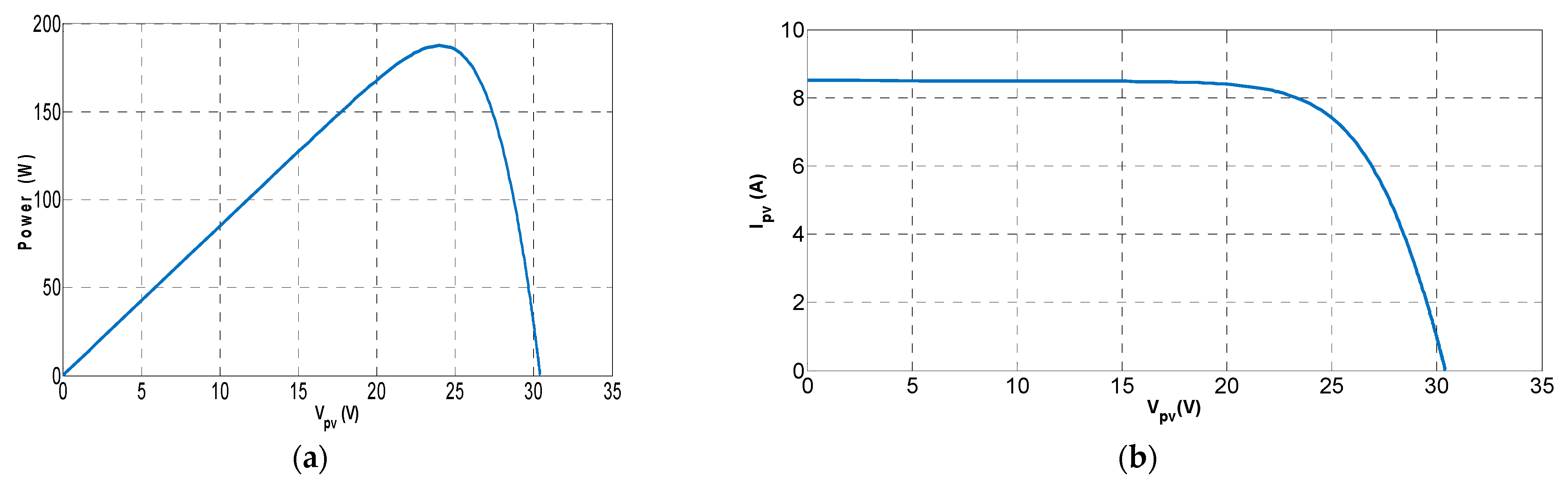
Figure 1. Structure of the studied PV system, where I PV and V PV denote its current and voltage.
Mathematics 10 02128 g001
Figure 2. Electrical equivalent circuit of the PV cell.
Mathematics 10 02128 g002
Figure 3. Electrical scheme of the studied system, where C is a capacitor, L is an inductor, I L is the inductor current, and S T ,   S D are a transistor and a diode of the step-down converter, respectively.
Mathematics 10 02128 g003
Figure 4. PV (a) and IV (b) characteristics of the PV module.
Mathematics 10 02128 g004
Figure 5. PV system’s physical characteristic radiance trajectory simulation.
Mathematics 10 02128 g005
Figure 6. System dynamics using I/O linearization controller for: (a) Motor pump current, (b) motor pump angular speed, (c) motor pump voltage, (d) DC converter inductance current, and (e) control input stabilization.
Mathematics 10 02128 g006
Figure 7. I/O control performance considering unmeasured random and matched disturbances for: (a) Motor pump current, (b) motor pump angular speed, (c) motor pump voltage, (d) DC converter inductance current, (e) control input stabilization.
Mathematics 10 02128 g007
Figure 8. Second-order sliding mode control performance considering unmeasured random and matched disturbances for: (a) Motor pump current, (b) motor pump angular speed, (c) motor pump voltage, (d) DC converter inductance current.
Mathematics 10 02128 g008
Figure 9. Characteristics of the SMO convergence.
Mathematics 10 02128 g009
Figure 10. Block diagram of the SMO-SOSM-I/O FBL controller.
Mathematics 10 02128 g010
Figure 11. Motor pump current under the indicated scheme.
Mathematics 10 02128 g011
Figure 12. Inductance current of the DC converter under the indicated scheme.
Mathematics 10 02128 g012
Figure 13. Motor pump voltage under different circumstances under the indicated scheme.
Mathematics 10 02128 g013
Figure 14. Motor pump angular speed under the indicated scheme.
Mathematics 10 02128 g014
Figure 15. Control signals under the indicated scheme.
Mathematics 10 02128 g015
Figure 16. Simulation of a real profile of the natural irradiance around the value of 1000   W / m 2 .
Mathematics 10 02128 g016
Figure 17. Dynamics of the motor pump with FBL control ignoring disturbances for: (a) Motor pump current, (b) motor pump angular speed. (c) motor pump voltage, (d) DC converter inductance current, (e) control input stabilization.
Mathematics 10 02128 g017aMathematics 10 02128 g017b
Figure 18. Dynamics of the motor pump with FBL control including disturbances for: (a) Motor pump current, (b) motor pump angular speed, (c) motor pump voltage, (d) DC converter inductance current. (e) control input stabilization.
Mathematics 10 02128 g018aMathematics 10 02128 g018b
Figure 19. Motor pump current for the indicated scheme.
Mathematics 10 02128 g019
Figure 20. Inductance current of the DC converter for the indicated scheme.
Mathematics 10 02128 g020
Figure 21. Motor pump voltage for the indicated scheme.
Mathematics 10 02128 g021
Figure 22. Motor pump angular speed for the indicated scheme.
Mathematics 10 02128 g022
Figure 23. Control signal for the indicated scheme..
Mathematics 10 02128 g023
Table 1. PV module parameters.
DescriptionParameter
Power at the maximum power point ( P mpp ) 190   W
Voltage at the maximum power point ( V mpp ) 24.3   V
Current at the maximum power point ( I mpp )7.82 A
Open-circuit voltage ( V OC )30.6 V
Short-circuit current ( I SC )8.5 A
Number of cells per module50
Table 2. PV solar pumping system numerical parameters.
DescriptionValues
PV generator I PH = 4.4   A ;   I S = 52.75 × 10 6 A ; V T = 6.73   V
Capacitor C = 4000 × 10 6   Farad
The identified parameters of the DC motor R = 1.07   Ω ;   L = 0.05   Henry ;   J = 476 × 10 6 kg   × m 2 ;   F = 88 × 10 5   per   unit , K T = 14 × 10 4 ,   K B = 45 × 10 3 per   unit
Table 3. Parameters and settings of the SMO algorithm.
ParametersValues
q 50
W adaptive
V b 1 to 1
V c 1 to 0
Table 4. Controller gain tuning for several control inputs in the irradiance trajectory of Figure 4.
Time Slot(8–9 h)(9–10 h)(10–11 h)(11–14 h)(14–15 h)(15–16 h)
I/O FBL control10.5010.159.348.0010.0111.00
Decoupling I/O FBL10.339.899.228.758.638.10
SOSM control8.007.747.106.687.007.50
SMO control4.353.563.002.883.453.72
Table 5. Values of the RMSE for the indicated aspects.
Time Slot(8–9 h)(9–10 h)(10–11 h)(11–14 h)(14–15 h)(15–16 h)
I/O FBL control11.7510.129.949.018.517.20
Decoupling I/O FBL20.2319.9119.4518.1717.26316.51
SOSM control17.0015.8413.12311.3619.978.85
SMO control109.018.26.0754.973.762
Publisher’s Note: MDPI stays neutral with regard to jurisdictional claims in published maps and institutional affiliations.

