A Compact Parallel Pruning Scheme for Deep Learning Model and Its Mobile Instrument Deployment

Abstract

In the single pruning algorithm, channel pruning or filter pruning is used to compress the deep convolution neural network, and there are still many redundant parameters in the compressed model. Directly pruning the filter will largely cause the loss of key information and affect the accuracy of model classification. To solve these problems, a parallel pruning algorithm combined with image enhancement is proposed. Firstly, in order to improve the generalization ability of the model, a data enhancement method of random erasure is introduced. Secondly, according to the trained batch normalization layer scaling factor, the channels with small contribution are cut off, the model is initially thinned, and then the filters are pruned. By calculating the geometric median of the filters, redundant filters similar to them are found and pruned, and their similarity is measured by calculating the distance between filters. Pruning was done using VGG19 and DenseNet40 on cifar10 and cifar100 data sets. The experimental results show that this algorithm can improve the accuracy of the model, and at the same time, it can compress the calculation and parameters of the model to a certain extent. Finally, this method is applied in practice, and combined with transfer learning, traffic objects are classified and detected on the mobile phone.

1. Introduction

Because of the remarkable achievements of deep neural network in computer vision, it has been widely studied and applied. However, with the increase of depth, its memory occupation and hardware requirements also increase, so its application is limited. To solve these problems, the concept of model compression is put forward. The methods of model compression include low-rank decomposition, quantization, pruning and lightweight network structure, etc. Pruning, as one of the effective methods of model compression, has been widely studied and used. It can reduce the memory consumption of the network model and the amount of calculation under the condition that the accuracy of the model is not significantly reduced or even slightly improved.

It is found that the earlier pruning is to simplify the network by pruning the weight, remove the unimportant neurons, and retrain the network until it converges. The compression model proposed by Han et al. [1] achieved a compression ratio of 35 times on AlexNet. In China, there is also much research on weight pruning. Gong Kaiqiang et al. [2] proposed a neural network compression method based on network pruning combined with tensor decomposition based on statistics, selecting mean and variance as the basis for evaluating the contribution of weight value, which is conducive to the deployment of model in resource-constrained embedded devices. Wang Zhongfeng et al. [3] took gradient as the basis for evaluating the importance of weights, removed the corresponding weights of gradients less than the threshold value in the model, and recovered the loss of model capacity through retraining. However, the pruning of weights will lead to a large number of irregular zeros in the network, the convolution kernel becomes a sparse tensor, and the model tends to be unstructured. Li et al. [4] designed the channel-pruning algorithm. As a structured pruning algorithm, channel pruning measures the importance of convolution kernels by designing standards, and completely cuts off unimportant convolution kernels and their corresponding feature graphs, so that most of the decentralization values will not be cut off and sparse tensors will be left. Liu et al. [5] proposed network slimming, focusing on the scaling factors in the batch normalization layer, and imposing regular constraints on them during training, so that the model can be continuously adjusted to the sparse channel structure in the training. The same point is that the pruned parameters will be permanently removed from the model and will no longer participate in reasoning and training. Although most parameters in the network are redundant, unstructured pruning algorithm will still permanently remove some key parameters. No matter what evaluation criteria are adopted, it is difficult to avoid false pruning, which will inevitably lead to the loss of information. Compared with unstructured pruning algorithms, the purpose of structured pruning is to retain the ability of the pruned part and avoid the reduction of model capacity caused by permanent pruning. The soft filter pruning proposed by He et al. [6] is a typical structured soft pruning algorithm, which allows the truncated convolution kernel to participate in the subsequent iteration update.

However, the uniqueness of the structured pruning algorithm also restricts its ability to compress the network. Because the structured pruning algorithm selects the activated convolution kernel according to the characteristics of the input image, considering that the input image is unknown and the activated convolution kernel is also unknown, the convolution kernel is difficult to permanently remove, which also leads to the network compression ratio being significantly lower than that of the unstructured pruning algorithm. Based on a series of problems existing in structured filter pruning, this paper proposes a parallel pruning algorithm based on image preprocessing, which can effectively further compress and optimize the model. The main work of this paper is as follows:

(1)

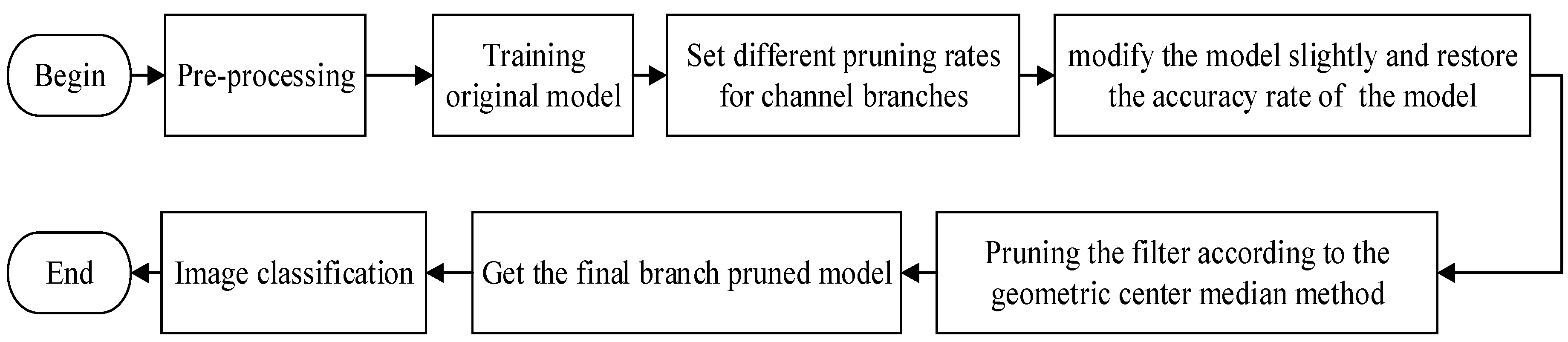
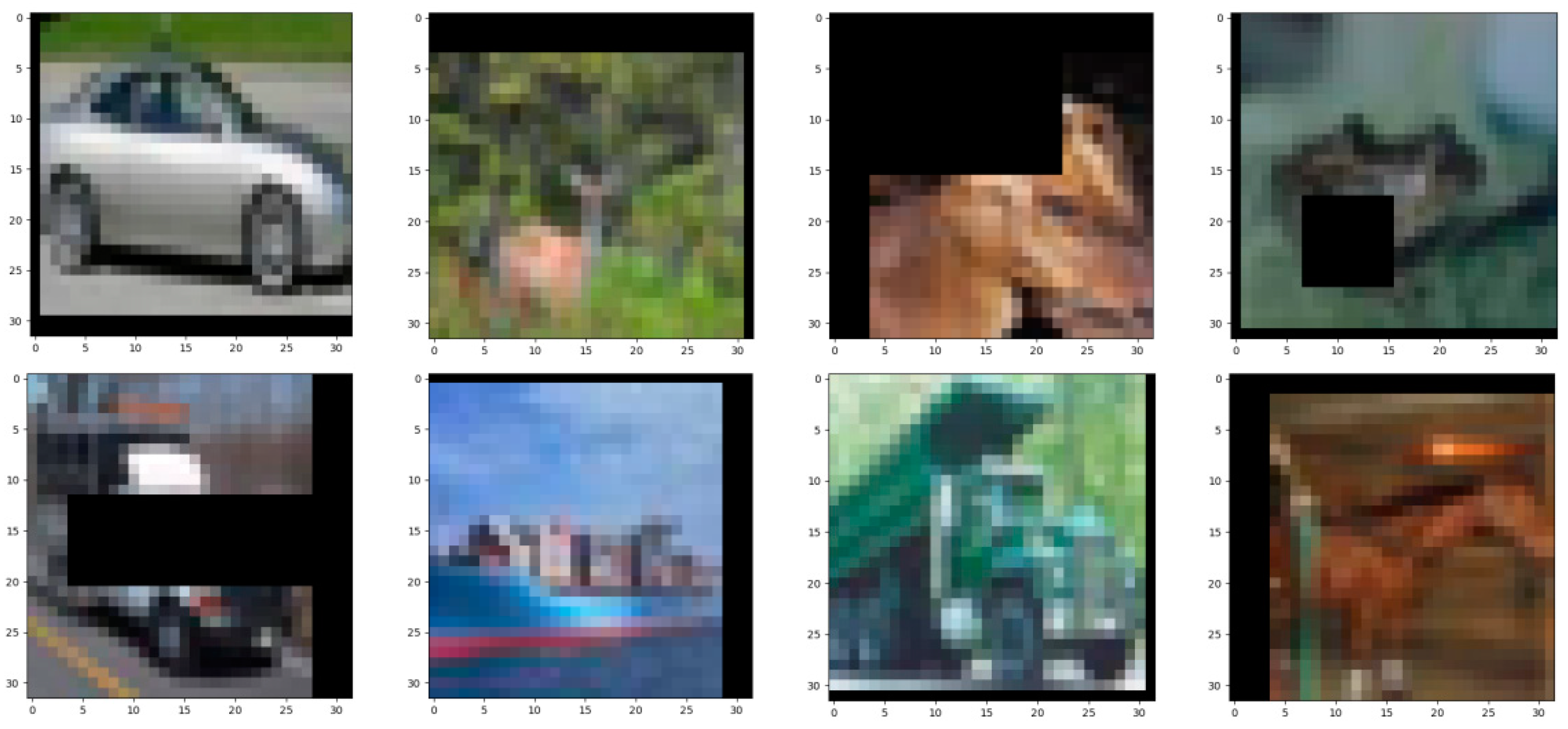
In this paper, the random-erasure algorithm in the image preprocessing method is used to preprocess the data set to obtain images with different occlusion degrees, which further increases the number of training samples, which greatly improves the generalization ability of the network and reduces the risk of over fitting.

(2)

A parallel pruning algorithm combining channel pruning and filter pruning is proposed. Firstly, according to the restriction of compression capacity in structured pruning, the channel pruning method is adopted to permanently remove some parameters in the depth neural network, so as to reduce the amount of calculation and maintain the accuracy of model classification as much as possible. Secondly, in order to obtain a better compression effect, the filter pruning method is used for further compression optimization, and the network is pruned without removing the model parameters.

(3)

Combining the characteristics of channel pruning and filter pruning, the two are organically combined to maintain the balance between the accuracy and complexity of the model. The network compressed by this pruning method is applied to the mobile terminal to realize the classification and real-time target detection of the mobile terminal.

2. Related Work

2.1. Introduction of Deep Convolutional Neural Network

The related research of CNN first started in the 1980s, and the time delay network (TDNN) was the first CNN proposed by researchers. Later, translation-invariant artificial neural network, LeNet, LeNet-5 and so on were successively proposed. The object to be studied in this paper is deep convolutional neural networks (CNNs), which is the deep structure of CNN. Typical deep convolution neural networks include ZFNet, proposed in 2013, VGGNet and GoogLeNet, proposed in 2014, and ResNet, proposed in 2015; then ResNeXt and DenseNet were proposed, and these networks have achieved good results in computer vision tasks. According to the research content of this paper, this paper selects different depths of VGGNet, ResNet and DenseNet for experiments. This paper mainly introduces the related structures of these three networks.

The VGG model is a deep convolutional neural network developed by the Visual Geometry Group of Oxford and Google Company in 2014 [7], which mainly proves that increasing the depth of the network can affect the final performance of the model to a certain extent. There are six different hierarchical structures of VGGNet, but, on the whole, these structures have one thing in common: they all contain five groups of convolution operations, all of which use 3 × 3 convolution kernels, and each group of convolution operations will be followed by a 2 × 2 Maxpool layer and finally three FC (fully connected) layers [8].

VGGNet can be said to be a network developed from AlexNet, and now VGG16 and VGG19 are the most widely used ones. Generally speaking, compared with other networks, the structure of VGGNet is very simple and clear. The whole network uses the same size of convolution kernel (3 × 3) and maximum pool layer (2 × 2). However, there is a problem that VGG will consume more computing resources in the process of using it, and it needs a lot of parameters to learn, which will lead to excessive memory occupation. For example, VGG16 contains 138,340,000 parameters, consumes more than 500 MB of storage space, and just classifying a single picture requires 30.94 billion floating-point operations [9]. In the VGGNet model, most of the parameters are from the first FC layer. However, VGG has three fully connected layers.

Then, in order to solve the problem of network degradation, researchers put forward the deep residual network ResNet in 2015, which solved the problem that the deep network is difficult to train by using the method of cross-level connection to fit the residual term, and increased the number of layers of the network to an unprecedented scale. In PyTorch, five structures of ResNet network are provided. Among them, the residual network with 152 layers needs to update its parameters, which is eight times that of the VGGNet model [10], but the complexity of the network is lower than that of ResNet-152. Moreover, in the image classification competition, ResNet achieved good results.

In ResNet, according to the types of Blocks, these five ResNets with different depths are divided into two categories: one is the residual network based on BasicBlock, that is, the shallow network resnet-18,34, which is composed of BasicBlock; the other is the residual network based on Bottleneck, that is, deep networks Resnet-50,101,152 and even deeper networks, all of which are composed of Bottleneck. Blocks are like building blocks. Several blocks can form each layer in the network, and these layers form the whole network. No matter how deep the ResNet network is, it is composed of four layers [11] (not counting the initial 7 × 7 layers in the network).

DenseNet was proposed in 2017. Instead of improving the network performance from the perspective of increasing the network depth and width, DenseNet looks for a breakthrough from the perspective of features. Using the idea of feature reuse and Bypass setting, DenseNet not only reduces the amount of network parameters and strengthens feature transmission, but also alleviates the gradient decline to a certain extent. When the structure of DenseNet network was first proposed, it was very similar to ResNet. At the beginning, it was a large-scale convolution, followed by a maximum pool, followed by several dense blocks and transition layers, and finally a pool layer and FC layer.

2.2. Image Preprocessing

In the process of image classification and recognition, image preprocessing is the operation before feature extraction, segmentation and matching of input images. The reason why, during training, the image should be preprocessed first is to remove the information in the image that has nothing to do with the extracted features, then repair the real and effective information in the image, enhance the verifiability of the associated information and greatly simplify the data, thus improving the reliability of feature extraction, image segmentation, matching and recognition [12]. In the process of deep network model classification training, on the one hand, with the deepening of the model layers, the model over-learns the details in the training data [13]. On the other hand, although it performs well in the training data set, when a new data set is used to test the network, the effect may be very poor, which leads to poor generalization performance of the model and over-fitting. In order to solve the above problems in the training process, image preprocessing method is used to expand the dataset, and random transformation method is used to increase the number of training samples and improve the generalization ability of the model.

During this period, many image enhancement methods and regularization methods have been proposed, such as random flipping, random cropping, dropout, batchnormal and so on. However, a new problem has arisen. In the uncovered data set, that is, all the targets are clearly visible, and the learned network may obtain higher accuracy; but, the adaptability of the network is limited, and there may be no way to identify those covered objects [14]. Therefore, in order to solve the problem of poor generalization ability of network caused by occlusion, a new image enhancement technology—random-erasure algorithm, referred to as RE—is proposed.

In the process of image preprocessing, the RE algorithm will randomly select the rectangular area to be occluded from the image, and use the random number to erase the pixel value of the selected rectangular area, so as to generate a training set with masking effect, and then train and test it. This method will reduce the risk of good performance in the model training process and poor performance in the test, and make the model stable for masking.

2.3. Network Pruning

As one of the methods of model compression, network pruning is both fast and effective. Generally speaking, pruning can be divided into two categories. One is unstructured pruning. The other is structured pruning, that is, pruning of filters, channels and layers. One of the most important shortcomings of unstructured pruning methods (that is, directly pruning the weights) is that the obtained weight matrix is sparse, and if there is no dedicated hardware or library, it cannot achieve the effect of compression and acceleration. On the contrary, structured pruning is pruning at the level of filters, channels or layers. Because the original convolution structure remains after pruning, it does not need special hardware or library to realize it. Therefore, generally speaking, structured pruning is the most popular pruning method among researchers at present.

According to the way of structured pruning, it can be roughly divided into channel pruning, filter pruning and layer pruning, and channel pruning is the most popular structured pruning, because it runs at the finest level and is still suitable for the traditional deep learning framework. Filter pruning is a higher level of pruning than channel pruning, which will not destroy the structure of the network and can effectively reduce the size of the network.

However, the uniqueness of the structured pruning algorithm just limits its effect of compressing the network. Because the structured pruning algorithm selects the activated convolution kernel according to the characteristics of the input image, considering that the input image is unknown and the activated convolution kernel is also unknown, it is difficult to permanently remove the convolution kernel, which also leads to the obvious lower network compression ratio than the unstructured pruning algorithm. Therefore, relatively speaking, directly pruning the model at the filter level may increase the loss of information and the possibility of false pruning. Based on a series of problems existing in structured filter pruning, this paper proposes a parallel pruning algorithm based on image preprocessing, which organically combines channel pruning with filter pruning, and performs parallel pruning operation on the model from both vertical and horizontal angles to maximize the optimization of model parameters.

2.4. Transfer Learning

In deep learning, it is a very common method to use pre-training model as the beginning of model training. As we all know, the pre-training model is a model that has been trained with large data sets. Usually, these trained models have already consumed huge time cost and calculation cost at the beginning of training, so in the following specific computer vision tasks and natural language processing tasks, there is no need to spend a lot of time and resources to train the models, which brings great convenience to the completion of the tasks. However, the pre-training model also has shortcomings in the use process. The disadvantages are that the model is large, the corresponding calculation amount and parameters are too large, and the structure of the model is fixed. It is difficult to change the network structure, and then there are scenarios that will limit the application of the model. Therefore, in most cases, we usually train the model from scratch. However, due to the limitation of hardware resources, some small data sets are usually used when training models, and the trained models often fail to achieve the expected results. To solve this problem, the concept of transfer learning has been put forward. Learning can transfer the knowledge learned from large data sets to related problem research.

Transfer technology is a deep learning method put forward in 2005. Its purpose is to take the model developed for task A as the starting point and re-apply it in the process of developing the model for task B. According to the way of learning, migration methods can be divided into the following categories: sample-based migration, feature-based migration, network-based migration and relationship-based migration [15]. At present, the most commonly used transfer learning method is the pre-training model method.

3. Parallel Pruning Algorithm Based on Image Preprocessing

3.1. The Random-Erasure Algorithm in Image Preprocessing Is Introduced to Preprocess the Data Set

In deep learning, in order to reduce the over-fitting problem of deep neural networks, it is necessary to increase the amount of data. Then, it is very important to enhance the data of the input image, and the enhanced data is of great significance to the classification of the model. In the process of data enhancement, commonly used methods mainly include contrast transformation, scale transformation, flip transformation and noise disturbance [16].

When there is no occlusion in the image, the model can better learn the convolution features, and can achieve good results when testing the image. However, due to the limited generalization ability of the model, the model may not recognize the objects in the image for a large number of pictures. At this time, it is necessary to partially occlude the image. This paper introduces the data enhancement algorithm of random erasure in image preprocessing to preprocess large-scale image data, hoping to reduce the risk of model over fitting and finally improve the generalization ability of the model [17]. This is conducive to model training and feature extraction. The specific process of the random erasure algorithm is as follows.

In the training of the model, the random erase (RE) data enhancement algorithm will erase the pixels of the selected area in the picture with a certain probability. For a small batch of images, it is assumed that the probability that the images $M$ are randomly erased is $q$, and the probability that they remain unchanged is $1-q$. In this process, the random-erasure algorithm will have different effects on the training data. When the random-erasure algorithm is executed, firstly, a rectangular area $R_e$ is randomly selected in the image, and the pixels in the area are erased with random numbers [18]. Assuming that the area of the image used for training is $A$, then:

$$A=W\times H$$

(1)

where $W$ is the width of the image and $H$ is the height of the image.

The area of the erased rectangular area is initialized to $A_e$, where the size of $A_e/A$ is between $A_1$ and $A_h$. The aspect ratio of the erased rectangular area is randomly initialized, and the value is between ${\beta }_1$ and ${\beta }_2$. The height and width of the erased rectangular frame are:

$$H_e=\sqrt{S_e\times {\beta }_e}$$

(2)

$$W_{\mathrm{e}}=\sqrt{\frac{A_{\mathrm{e}}}{{\beta }_{\mathrm{e}}}}$$

(3)

where the height of the erased rectangular frame is $H_e$, the width is $W_e$, the height–width ratio is ${\beta }_e$, and the area is $A_e$. In image $M$, a point $Z$ is initialized randomly and $Z=(x_e,y_e)$, if the following conditions are true:

$$x_e+W_e\le W$$

(4)

$$y_e+H_e\le H$$

(5)

Take the area $A_e=(x_e,y_e,x_e+W_e,y_e+H_e)$ as the selected rectangular area. Otherwise, the above process is repeated until a suitable rectangular area $A_e$ is selected. Then, each pixel in the selected rectangular area, that is, the area $A_e$ to be erased, is assigned a random value ranging from 0 to 255.

As a lightweight image preprocessing method, random erasure can be deployed in various convolutional neural networks without any additional parameter learning and memory consumption, and it is a supplement to the existing data enhancement and regularization methods. Therefore, the introduction of the random-erasure algorithm not only solves the generalization ability of the model, but also does not increase the parameters of the model.

3.2. Parallel Pruning Algorithm

After preprocessing the data set, the next thing to do is prune the model. Pruning and accelerating the deep convolution neural network can effectively reduce the memory consumption and computation of the network, and solve the problem that the depth model is difficult to be applied to resource constrained devices [19]. In order to remove the redundant parameters in the model as much as possible, next, we will briefly introduce the two pruning strategies involved:

(1)

Channel pruning method based on batch normalization layer

Compared with filter pruning, the compression ratio of channel pruning is larger. This is one of the reasons why this paper chooses channel pruning as the initial thinning of the model. The essence of channel pruning [5] is to use the scaling factor learned by the batch normalization layer as the basis for judging the channel importance, which simplifies the process of channel importance calculation. Because the scaling factor is a parameter automatically learned in the process of model training, it can also be said to be adaptive pruning to some extent. Specifically, the idea of channel pruning is to introduce a scaling factor for each channel and multiply it by the output of that channel. Then, combining the weight of the training network with the introduced scaling factor, the latter is subjected to sparsity regularization. Finally, the small factor channel is trimmed and the trimmed network is fine-tuned. The objective function of channel pruning is [20]:

$$L={\displaystyle \sum _{(x,y)}l(f(x,W),y)+\lambda {\displaystyle \sum _{\gamma \in \mathrm{\Gamma }}\mathrm{g}(\gamma )}}$$

(6)

where $(x,y)$ represents the input and output of training, $W$ is the training weight, the first sum term corresponds to the normal training loss of the network, $g(\gamma )$ is the sparsity penalty for the scaling factor, and $\lambda$ is used to balance these two terms.

Using the $\gamma$ parameter in the batch normalization layer as the scaling factor required for channel pruning, its biggest advantage is that it will not bring additional computational overhead to the network. Because the batch normalization layer can accelerate network convergence, it has been widely used in various network structures. The batch normalization layer is usually placed behind the convolution layer to normalize the output characteristics of the convolution layer, so that each layer structure in the network can learn by itself and is slightly independent from other layers [21]. In the learning process, the batch normalization layer will obtain two parameters, scaling coefficient and offset coefficient, and then adjust the normalized feature data according to these two parameters, so that the feature value can learn the feature distribution of each layer [21]. The batch normalization layer performs the following transformation:

$$F_{out}=\gamma \frac{F_{in}-\mu }{\sqrt{\sigma +\epsilon }}+\beta$$

(7)

In Formula (7), $F_{in}$ represents the input, $F_{out}$ represents the output, $\mu$ represents the average of the input activation values, and $\sigma$ is the variance of the input activation values, and $\gamma$ and $\beta$ are the scaling coefficients and offset coefficients of the corresponding activation channels. In the batch normalization layer, the learned parameter $\gamma$ corresponds to each active channel, so $\gamma$ can be used to judge the importance of each active channel.

After channel-level sparsity training, a sparse model can be obtained. There are many scaling factors close to zero in this model, and then the channels with these scaling factors close to zero are pruned. Prune the channel by using a global critical value across all layers, which is defined as a percentage of all scale factor values. For example, set the threshold percentage to 70%, and then trim 70% channels with a low scale factor. In this way, we can obtain a compact network with fewer parameters and calculation operations and less memory consumption.

(2)

Filter pruning method based on geometric median

Next, the second pruning strategy to be introduced is filter pruning. This pruning method is mainly based on geometric median. The main idea is to prune redundant filters, not those that are relatively unimportant. It selects those filters that contribute the most substitutability. According to the characteristics of geometric median (GM) [22] of filters in the same convolution layer in the model, the nearby filters can be represented by residual filters. The algorithm process is as follows:

Assuming that the network to be pruned is $L$ layer, $C_i$ represents the number of input channels in the $i$ convolution layer, $C_{i+1}$ represents the number of output channels in the $i$ convolution layer, and $F_{i,j}$ represents the $j$ filter in the $i$ convolution layer. In layer $i$, find the filter closest to the geometric median of this layer, and its formula is as follows:

$$F_{i,j^{*}}=\arg \min {\Vert F_{i,j^{’}}-x^{GM}\Vert }_2,s.t.j^{’}\in [1,C_{i+1}]$$

(8)

Then, $F_{i,j^{*}}$ can be represented by other filters in the same layer, so trimming them has little impact on network performance. Where $x^{GM}$ is the geometric mean. As the geometric mean is a classical robust estimation of data centrality in Euclidean space, the geometric mean is used to obtain the common information of all filters in a single layer, and its calculation is as follows:

$$x^{GM}=\underset{x\in R^{C_i\times K\times K}}{\arg \min }{{\displaystyle \sum _{j^{’}\in [1,C_{i+1}]}\Vert x-F_{i,j^{’}}\Vert }}_2$$

(9)

Both pruning methods belong to structured pruning, but there are some differences between them. The difference is that the compression ratio of filter pruning is obviously smaller than that of channel pruning, that is, the compression ratio of filter pruning is limited. Secondly, usually, channel pruning will directly delete unimportant channels according to the pruning strategy, so the memory occupation of the model will be reduced a lot after pruning, while the filter pruning will not be directly deleted—only the redundant parameters will be set to zero, so the memory occupation of the model will hardly change after pruning. Based on these two differences, this paper proposes a parallel pruning algorithm. In this algorithm, the channel pruning based on batch normalization layer and the filter pruning based on geometric median are fused, and the model is pruned horizontally and vertically in parallel, which greatly reduces the parameter redundancy in the model, reduces the memory occupancy of the model after pruning, and improves the compression ratio of the model.

3.3. Algorithm Flow Chart

Through the research of channel pruning and filter pruning methods, it can be seen that only one pruning strategy, such as channel pruning or filter pruning, is adopted to optimize and accelerate the depth network model, and there are still many redundant parameters in the optimized model [19]. Usually, a deep convolution neural network contains hundreds of channels, and each channel describes different aspects of the previous layer. As far as the structure level of the network is concerned, the channel and convolution kernel are located in the next layer of the filter, while the concepts of the filter and the layer are at the same level. Therefore, directly pruning the filter will greatly cause information loss and affect the accuracy of model classification, and the filter pruning method limits the compression ratio of network compression. In order to improve the compression ratio and further optimize the network model, a parallel pruning method combining channel pruning and filter pruning is proposed.

Firstly, the training data is preprocessed, and the generalization ability of network learning is improved by random erasing methods. Secondly, channel pruning method is used to train the model at channel level. The batch normalization layer is widely used in deep neural networks, such as VGG and DenseNet, because it can accelerate network convergence. According to the scaling factor of the batch normalization layer, the channels with low importance are pruned to obtain a more compact network compared with the original model, but there are still many redundant parameters in the compressed network. Finally, in order to further optimize the compressed model, the redundant filters are trimmed by the filter pruning method. At this time, the convolution layer is regarded as a three-dimensional space, and the filters in it are regarded as points in the space. Because the geometric median is a classical robust estimation of data centrality in Euclidean space, the geometric median is used to obtain the common information of all filters in a certain layer. Then, we calculated the distance from other filters to this geometric median, and found the filter closest to this geometric median. Then it could be considered that this filter is redundant and can be replaced by other filters and pruned. The algorithm flowchart is shown in Figure 1.

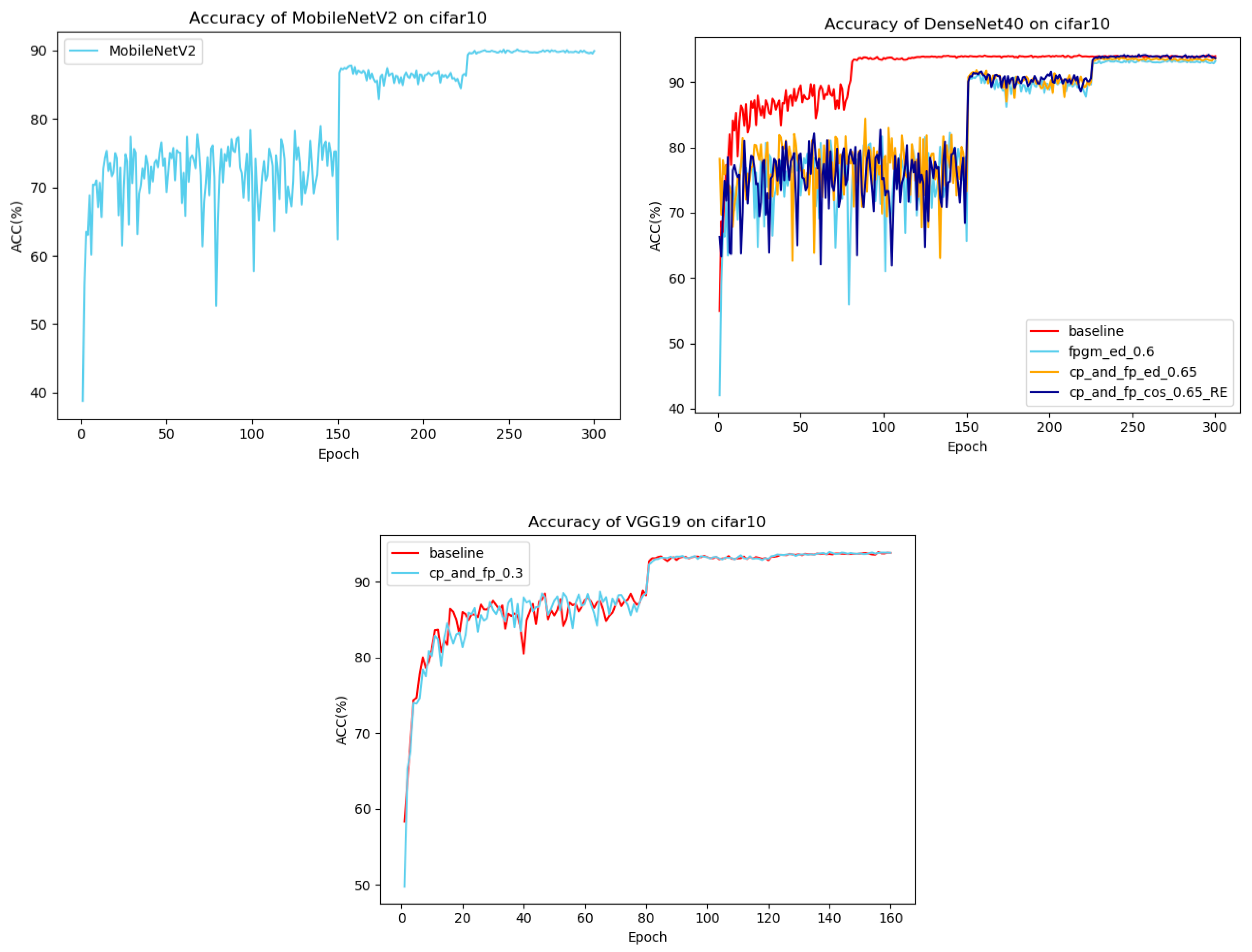
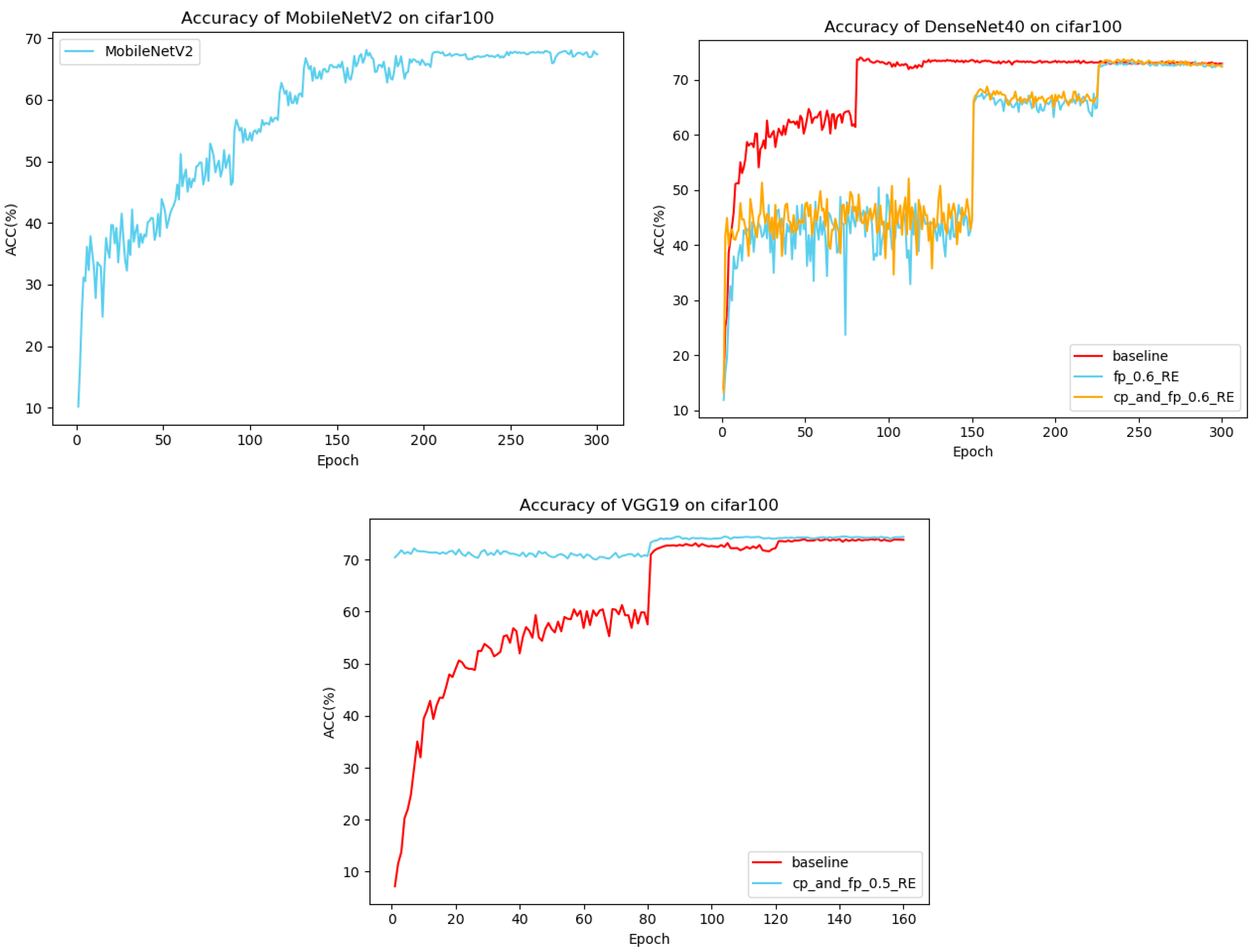
4. Experimental Results and Analysis

The experiment was conducted on a device with Ubuntu system, Intel Core i7 9750H processor and NVIDIA Ge Force GTX 1650 graphics card. The experimental environment is Pycharm 2019.2.4 (community edition), torchversion1.8.0 and CUDA version10.0.

In this experiment, CIFAR10 and CIFAR100 data sets are selected. CIFAR10 and CIFAR100 are both classic data sets used for image recognition. The CIFAR10 data set was collected and produced by Krizhevsky, etc. It contains 60,000 images with 10 categories. The CIFAR100 data set also contains 60,000 images. The difference between the two data sets is that CIFAR100 is divided into 100 categories, with 600 images in each category [23]. The images in CIFAR data set are all from real objects in reality, and they are all three-channel images. In these images, the size, characteristics and background of objects are different, so they have certain complexity and diversity. Compared with a single one-channel data set MNIST, which only contains handwritten numbers, CIFAR data set has more practical significance [23]. Furthermore, compared with the complex ILSVRC2012 dataset, CIFAR is relatively small in scale, not easily limited by the performance of equipment, and convenient for training.

During the experiment, the data set is preprocessed at first. Besides flipping, clipping and normalizing the data set, random erasing is also performed, which not only increases the diversity of data, but also enhances the generalization ability of the model. After randomly erasing the CIFAR10 dataset, the occlusion effect diagram generated by it is shown in Figure 2.

Next, pruning training is carried out on DenseNet40, VGG19 and other deep network models, so as to optimize the compression model parameters and calculation amount while slightly improving or not affecting the classification accuracy of the models. This experiment is a further improvement of the research method of pruning algorithm of depth separable filter based on PCA, which makes up for the shortcomings of its single model and data set experiment and method. A parallel pruning algorithm combined with image enhancement is proposed, and the above network is tested. After 300 rounds and 160 rounds of training respectively, the learning rate was set to 0.1, and the batch size was 64.

In this paper, the pruning experiments of VGG19 and DenseNet40 models are carried out by setting different pruning rates on the datasets of CIFAR10 and CIFAR100, keeping other parameters the same. The results are shown in

Table 1. Comparison of pruning effects of models VGG19 and DenseNet40 on CIFAR10 dataset.

Network	Method (Pruning Rate.%)	Test Acc (%)	Param (M)	Prune (Acc. %)	Flops (G)
VGG-19	Baseline	93.66	20.04	—	7.97
	LECNN (70%)	93.80	2.30	88.5	3.91
	Cp-and-FpRe (70%)	94.90	3.25	83.8	2.31
Densenet-40	Baseline	93.89	1.05	—	5.33
	LECNN (40%)	94.89	0.69	34.3	3.81
	FPGM (40%)	93.57	1.05	—	2.87
	Cp-and-Fp (40%)	94.04	0.88	—	—
	Cp-and-FpRe (40%)	94.99	0.88	16.2	2.49
	Cp (60%)	87.32	0.49	53.3	1.53
	Fp (60%)	93.43	1.05	—	—
	Cp-and-Fp (60%)	93.30	—	—	1.76
	Cp-and-FpRe (60%)	94.30	0.59	43.8	1.76
	Cp-and-Fp (65%)	93.77	0.59	—	—
	Cp-and-Fp-Cos (65%)	93.81	—	—	—
	Cp-and-FpRe (65%)	94.21	0.59	43.8	1.76
MoblieNetV2	—	90	4.133	—	6.08

The bold and highlights are experimental results of the proposed algorithm.

and

Table 2. Comparison of pruning effects of models VGG19 and DenseNet40 on CIFAR100 dataset.

Network	Method	Test Acc (%)	Param (M)	Prune (Acc.%)	Flops (G)
VGG-19	Baseline	73.26	20.08	—	7.97
	LECNN (50%)	73.48	5.0	75.1	5.01
	Cp-and-Fp (50%)	74.50	7.24	—	—
	Cp-and-FpRe (50%)	75.67	7.24	63.9	3.0
Densenet-40	Baseline	74.64	1.06	—	5.33
	Cp (40%)	74.72	0.66	37.5	3.71
	Fp (40%)	73.89	1.06	—	2.87
	Cp-and-Fp (40%)	74.90	—	—	—
	Cp-and-FpRe (40%)	76.40	0.76	28.3	2.49
MoblieNetV2	—	68.08	—	—	—

The bold and highlights are experimental results of the proposed algorithm.

. Table 1 shows the pruning results of VGG19 and DenseNet40 on CIFAR10, while Table 2 shows the pruning results on CIFAR100. Compared with the single channel pruning and filter pruning methods, the method proposed in this paper has a certain effect on reducing the calculation and parameter of the models. When the pruning rate is 70%, The parameters of VGG19 model are reduced by 83.8%, and the calculation is reduced by 71%, and the accuracy of the model is improved by about 1%, which provides a further possibility for its deployment on small devices. In Table 1 and Table 2, the experimental results of the lightweight network MobileNetV2 on CIFAR10 and CIFAR100 data sets are also given, and the change of its correct rate in the training process is drawn, as shown in Figure 3 and Figure 4. Because MobileNet itself is a lightweight structure specially designed for mobile terminals, this article does not prune it here.

In order to achieve better compression effect of the model, this paper prunes the model in parallel. By combining channel pruning, the restriction of filter pruning on compression ratio is improved and the compression ratio of the whole model is increased. As shown in Figure 3 and Figure 4, on the data sets of CIFAR10 and CIFAR100, after increasing the compression ratio of the models, the classification accuracy of the models DenseNet40 and VGG19 can still remain the same as the baseline, even slightly higher, which is in line with the experimental expectation.

5. Case Study

After pruning the model, the classification performance of the pruned model is verified by image classification experiments. The experimental results show that the method proposed in this paper effectively reduces the parameters and computation of the deep network model, greatly reduces the occupation of internal storage of the model, and improves the accuracy of model classification. This is only a theoretical study, and the classification effect of the pruned model in practical application remains to be studied. Image classification is simply a method of image processing. The classification of images is based on the different features of the images themselves in the image information [24]. Image classification is the core of computer vision and has been widely used in practice. However, for image classification, it is rarely applied to the mobile terminal, because most of the image classification models are very large, such as VGG, ResNet, DenseNet, etc., which all require high memory, so it is very difficult to deploy them to the mobile terminal. Therefore, the next content to be studied in this paper is the application of image classification based on a mobile terminal.

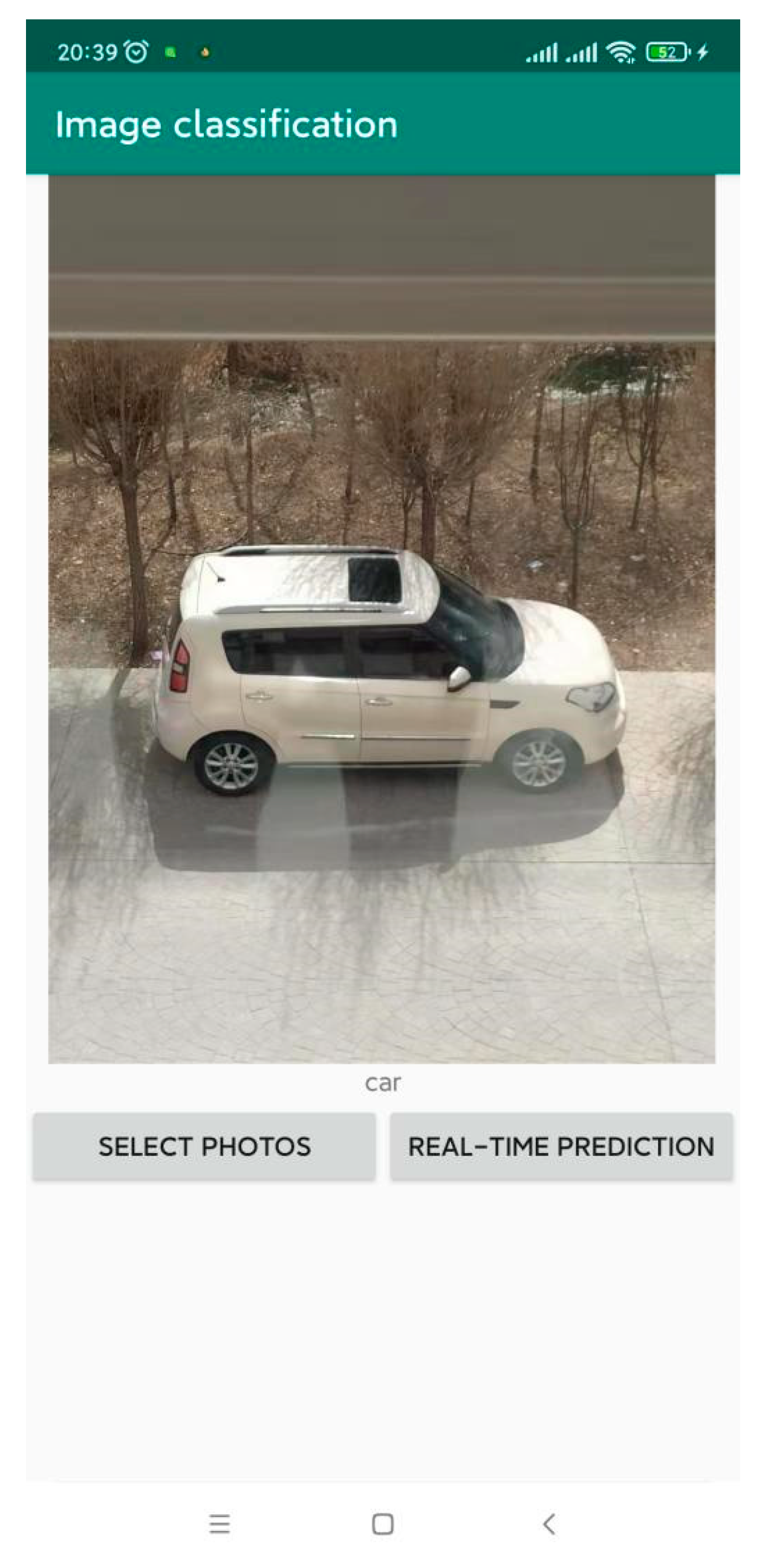
5.1. Image Classification Based on Mobile Terminal

The reason why the model is pruned is to facilitate its deployment on the mobile side. The process of image classification on the mobile terminal is as follows.

Firstly, the pruned model is trained on PyCharm, and the tag file corresponding to the training data set is generated during the training process. Then, the prediction file is called to test the model, and the format of the $Pth$ model file generated after the test is converted into a $pt$ file that can be deployed on the mobile terminal. Here, the first step to realize the classification of the model on the mobile side is completed.

The following is the experiment of the classification effect on the mobile terminal. Based on Android Studio platform, put the model converted in the previous step in the folder./app/src/main/assets, then connect the mobile terminal, open the USB debugging and installation, run the files, and classify the pictures. The final classification result is shown in Figure 5.

5.2. Mobile Traffic Object Detection Combined with Transfer Learning

The purpose of accelerating the optimization of the model is to maximize the application of the model, so that it cannot be limited by equipment and so on, and better serve the lives of the public. In order to make the compressed model have good generalization ability and be able to identify and detect targets well in different situations, this chapter proposes mobile traffic object detection based on transfer learning. Through transfer learning on the public driving dataset BDD100K, we build our own traffic object detection network.

5.2.1. Transfer Learning of BDD100K Dataset and YOLO Network

The data set used in this paper is BDD100K, published by the AI Lab of Berkeley University, and the data set BDD100K is the dataset related to traffic objects with the most images and the most extensive content at present. This sample set contains 100,000 video resources, and each segment is about 40 s, 720 p and 30 fps. We sampled the important frames in the 10th second of each video segment to obtain 100,000 pictures (picture size: 1280 × 720) and labelled them [25]. It contains 100,000 road boundary boxes, 100,000 driving ranges, 100,000 lane markings and 10,000 full-frame examples. Among them, the marked objects are: the uniform resource locator, category label, size (start coordinates, end coordinates, width and height), truncation, occlusion and traffic signal color of the source image [26]. There are 10 kinds of images, namely Bus, Light, Sign, Person, Bike, Truck, Motor, Car, Train and Rider. There are about 1,840,000 calibration boxes in total. These 100,000 pictures contain pictures of different climates, scenes and times, and there are clear and unclear pictures, which are large in scale and diverse [27], all of which are real driving scenes.

After introducing the data set, the following is the network YOLO, which is one of the classic target detection networks and has been widely studied and applied since it was put forward. As a fast, compact and effective open-source object detection network, compared with other models, it has stronger performance and good reliability. It is the first network that can predict the category and bounding box of the target object, and can predict multiple bounding box positions and categories at once. The biggest feature of YOLO is its fast detection speed. YOLO has been upgraded to v5 version up to now, showing its strong vitality from v1 to v5. YOLOv5 is used as the experimental network here. In this paper, YOLO is trained and pruned on a custom data set, and the specific process is not described here. What we want to say here is that YOLO network has its unique data set label format. The following is a study on the migration of the pruned network. The so-called transfer learning is to apply the knowledge learned in a certain scene or task to different but related scenes or problems.

During the training of custom data set, due to the insufficient amount of data and relatively single data, when doing target detection, for a certain scene, the detection effect is not ideal because of insufficient data, so it is very suitable for transfer learning. Therefore, in order to build our own traffic object detection network, this paper makes up for the lack of data in the early stage by transferring and learning the automatic driving data set BDD100K.

After the data set BDD100K and YOLO V5 model framework are prepared, the label format of the training sample is converted to YOLO format. The University of California, Berkeley, provides a tool for tag viewing and tag format conversion of BDD100K datasets. As there is no tool to directly convert BDD100K into YOLO format, one must first convert the label of BDD100K into the label format of coco data set, and then convert the coco label format into YOLO label format. You will obtain two .json files after the conversion. The following is to change the label format of training data and verification data into YOLO format. In the process of conversion, it should be noted that the positions of training and verification data set images, matching tag files and finally YOLO tags should be specified respectively. Then, one can start training the model and obtain the weight file of .pt.

5.2.2. Application of Mobile Object Detection

This chapter is to deploy the above-mentioned network to the mobile terminal to realize the real-time target detection of the mobile terminal. The process includes three modules, YOLOv5 target detection project file, ONNX model conversion tool and NCNN framework. The experimental environment is Android Studio 2020.3.1, the mobile device used is Android 11.0 and the screen resolution of mobile phone is 2340 × 1080. The experiment is carried out in the framework of PyTorch. Although the PyTorch framework is the mainstream deep learning development platform at present, there are still some shortcomings in the deployment. Therefore, this paper uses NCNN to deploy the PyTorch model to the mobile terminal.

NCNN is an open-source deep learning forward framework for mobile devices (especially Android) which is opened by Tencent. It only has forward calculation, so it cannot be trained and learned. It is necessary to input the network parameters that have been trained and learned by other frameworks. NCNN has been deeply considered for the application of mobile phones from the beginning of its development. It can be used on multiple platforms without relying on third-party support, and the speed of mobile phone processor is faster than the existing open-source architecture. In general, NCNN can be seen in reference [28].

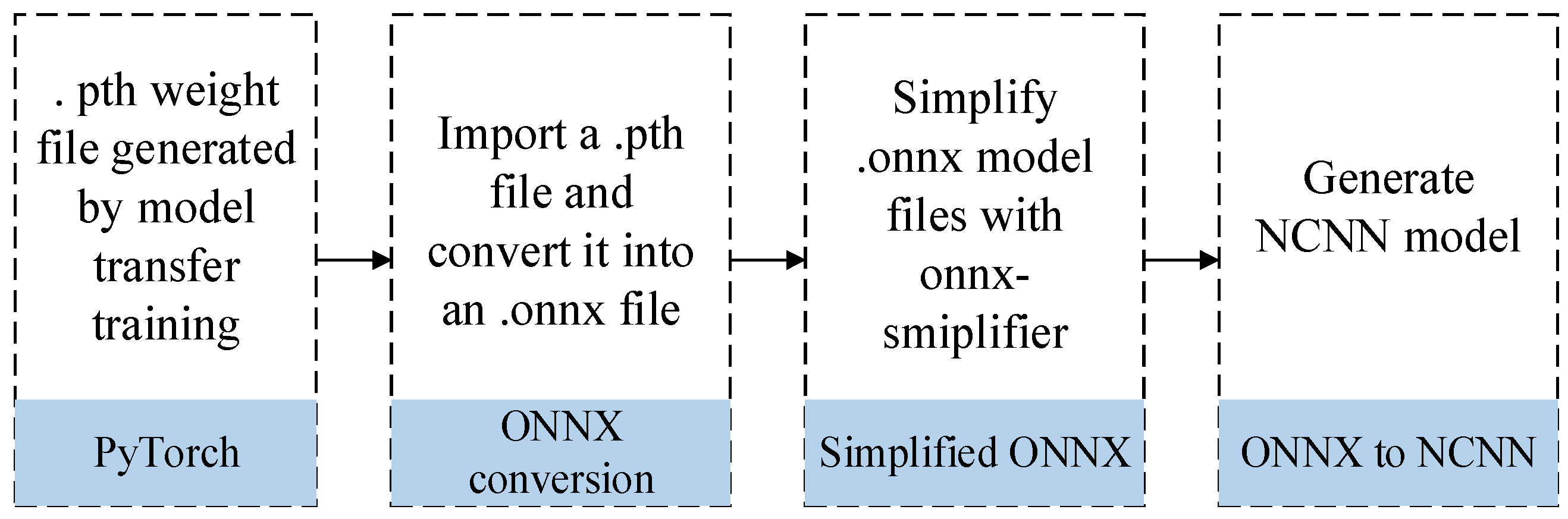
Model Transformation

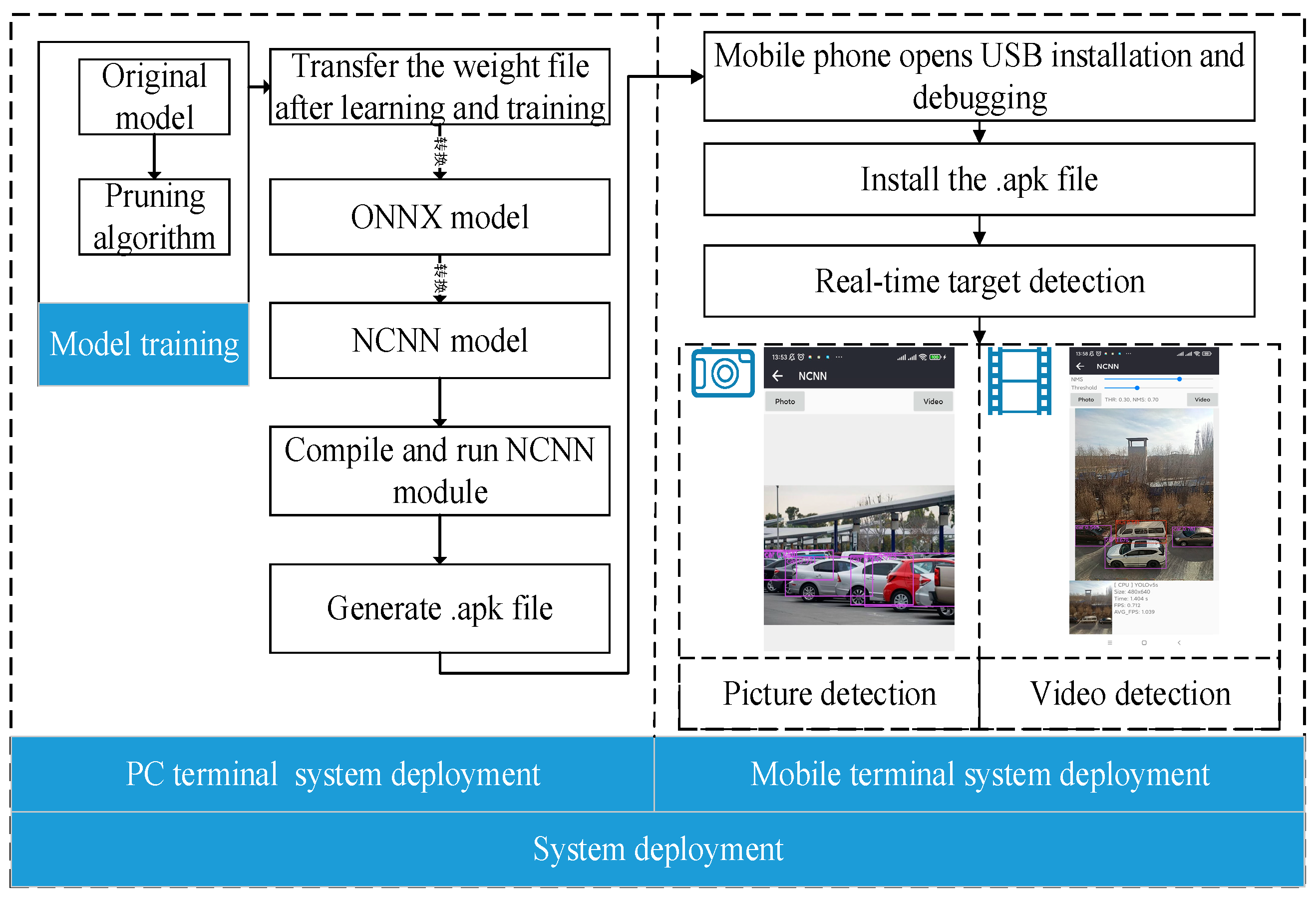
After transferring the model, to deploy it on mobile devices, it is necessary to transform the model.

First, we need to convert the trained model into ONNX, a unified format, and store it. It is a middleware in model transformation. Because there is no direct interaction between NCNN and PyTorch models. ONNX (Open Neural Network Exchange) is an open-file format specially designed for machine learning. It can be used to represent the standards of machine learning neural networks and preserve the learned models, which can make the networks transfer and interact among different architectures, such as Pytorch, Caffe2, MXNet, etc. The file generated after ONNX model conversion not only saves the weight of the network model, but also saves the structure information of the model, the input and output of each layer in the model and some other related information.

Then, the model in ONNX file format is converted into NCNN model. Before that, the model should be simplified to prevent the model from being uncompiled. Finally, the generated NCNN model contains two files (.param and .bin), .param is the configuration file of the model and .bin is the weight file of the model. The model conversion process is shown in Figure 6 below.

System Deployment

After converting the model, the whole PC and mobile system application deployment is started. Compile and run the converted NCNN model, and realize real-time traffic object detection on Android based on the compressed model YOLO. The system deployment is shown in Figure 7.

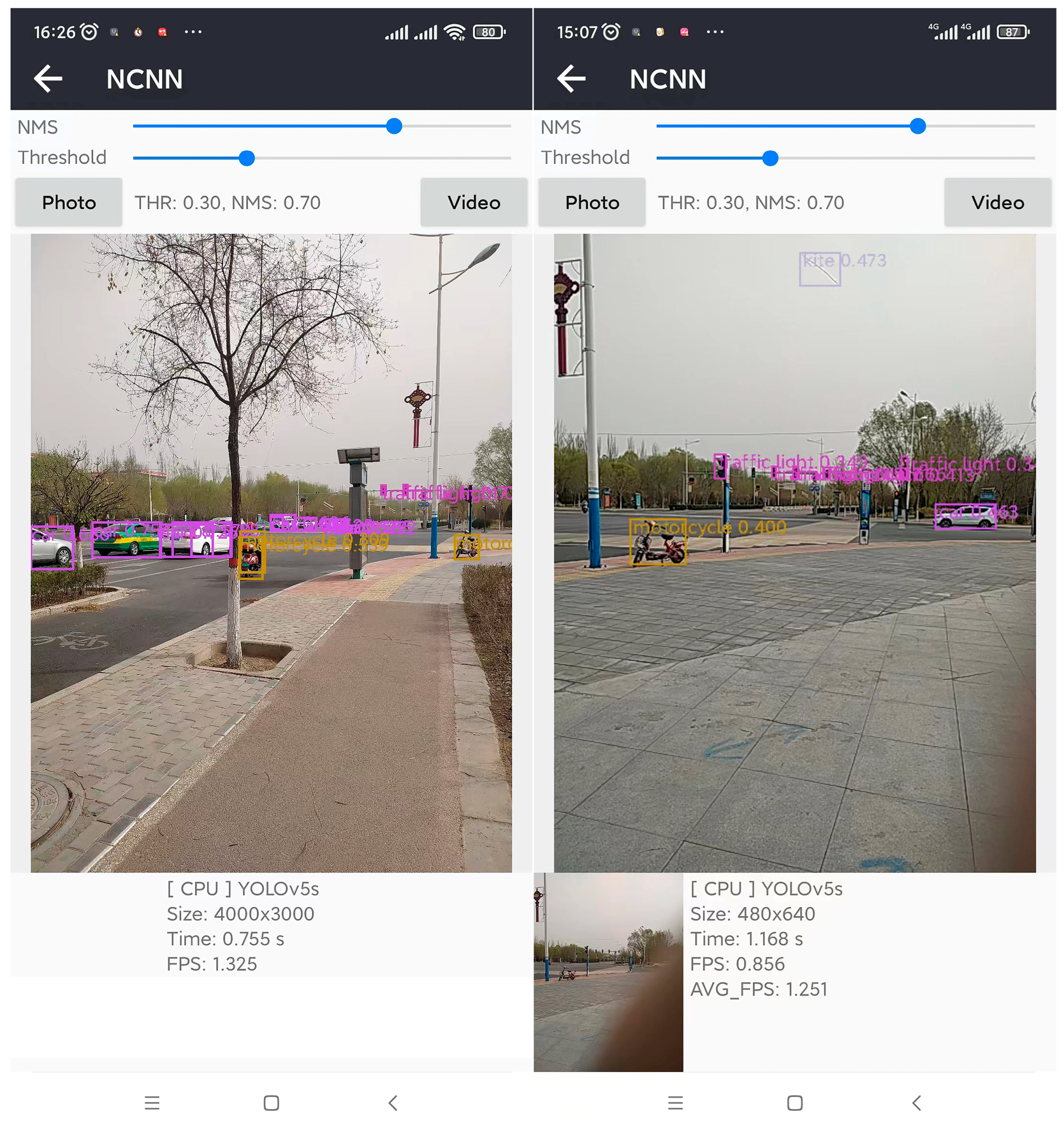
Traffic Detection and Recognition Effect

After building the framework, transforming the model and deploying the system, the next thing to do is to realize the object detection on the mobile terminal. In this paper, YOLOV5s, a target detection model, is used. By transferring and learning the large-scale driving data set BDD100K, traffic objects can be detected and identified. According to the situation, you can choose to detect both pictures and videos in real time. The detection and recognition effect are shown in Figure 8.

6. Conclusions

This paper presents a parallel pruning method based on image preprocessing. This algorithm combines the random-erasure algorithm with image preprocessing, and makes use of the respective advantages of channel pruning and filter pruning to evaluate the importance and redundancy of channel and filter. The main idea of the algorithm is to preprocess the data set, use a random-erasure algorithm, increase the number of training samples and enhance the generalization ability of the model. Secondly, the model is preliminarily thinned, and the channel importance is preliminarily evaluated through the parameters learned in the model training process, that is, scaling factor, and the channel with low importance is pruned. Then, the Euclidean distance is used to calculate the information distance of all filters in each convolution layer, and then the redundancy of filters is identified by the value of information distance of each layer, and the redundant filters are pruned. Here, the algorithm evaluates the importance of channels and filters from two directions. Finally, the algorithm performs experiments on multiple models on multiple data sets. The results show that this algorithm prunes the model, which further improves the performance of the model. This method is applied to the mobile terminal. By introducing transfer learning, traffic objects are classified and detected in real time.

References

1. Zhao, M.; Hu, M.; Li, M.; Peng, S.-L.; Tan, J. A Novel Fusion Pruning Algorithm Based on Information Entropy Stratification and IoT Application. Electronics 2022, 11, 1212. [Google Scholar] [CrossRef]
2. Gong, K.; Zhang, C.; Zeng, G. Convolutional neural network model pruning combined with tensor decomposition compression method. Comput. Appl. 2020, 40, 3146–3151. [Google Scholar]
3. Wang, Z.; Xu, Z.; Song, C.; Zhang, H.; Cai, Y. Deep network pruning algorithm based on gradient. Comput. Appl. 2020, 40, 1253–1259. [Google Scholar]
4. Li, H.; Kadav, A.; Durdanovic, I.; Samet, H.; Graf, H.P. Pruning Filters for Efficient ConvNets. arXiv 2016, arXiv:1608.08710. Available online: https://arxiv.org/abs/1608.08710 (accessed on 27 December 2021).
5. Liu, Z.; Li, J.; Shen, Z.; Huang, G.; Yan, S.; Zhang, C. Learning Efficient Convolutional Networks through Network Slimming. In Proceedings of the IEEE International Conference on Computer Vision (ICCV), Venice, Italy, 22–29 October 2017. [Google Scholar]
6. He, Y.; Dong, X.; Kang, G.; Fu, Y.; Yan, C.; Yang, Y. Asymptotic Soft Filter Pruning for Deep Convolutional Neural Networks. IEEE Trans. Cybern. 2019, 49, 4501–4564. [Google Scholar] [CrossRef] [PubMed] [Green Version]
7. Liu, J.; Chen, Q.; Amudula, E. Research on point target tracking technology based on correlation filtering and CNN. Laser Infrared 2021, 51, 244–249. [Google Scholar]
8. Zhang, X.; Wei, Y. Detection and extraction of key targets in driving scenes based on deep learning. J. East China Univ. Sci. Technol. 2019, 45, 980–988. [Google Scholar]
9. Guo, J. Research on Pruning Method of Deep Convolution Neural Network Model; Beijing Jiaotong University: Beijing, China, 2020. [Google Scholar]
10. Pang, S.; Huang, C. Research on Image Classification Based on Convolutional Neural Network. Mod. Comput. 2019, 23, 40–44. [Google Scholar]
11. Gao, Q.; Li, C.; Jin, X.; Li, Y.; Wu, H. Research on weed classification and model compression method in tea garden based on depth residual network. J. Anhui Agric. Univ. 2021, 48, 668–673. [Google Scholar]
12. Xie, X. Research on Driver Fatigue Detection Based on Machine Vision; Central South University: Changsha, China, 2010. [Google Scholar]
13. Zhang, W.; Sun, X.; Qiao, Y.; Bai, P.; Jiang, H.; Wang, Y.; Du, C.; Zong, H. Tobacco disease identification based on incidence v3. Acta Table Sin. 2021, 27, 61–70. [Google Scholar]
14. Jiang, Y.; Zhang, H.; Chen, L.; Tao, S. Image data enhancement algorithm based on convolutional neural network. Comput. Eng. Sci. 2019, 41, 2007–2016. [Google Scholar]
15. Lian, C.; Zhong, S.; Zhang, T.; Zhou, N.; Xie, M. Transfer learning classification of optical coherence tomography retinal images. Adv. Laser Optoelectron. 2021, 58, 270–276. [Google Scholar]
16. Guan, S.; Zhang, Q.Y.; Xie, H.; Qiang, Y.; Cheng, Z. Convolutional neural network model for CT image recognition. J. Comput. Aided Des. Graph. 2018, 30, 1530–1535. [Google Scholar] [CrossRef]
17. Jin, C.; Wang, H.; Chen, S. Pedestrian reidentification method based on random erasure pedestrian alignment network. J. Shandong Univ. 2018, 48, 67–73. [Google Scholar]
18. Yu, X.; Bing, X.; Meng, J.Z. Self-adaptive particle swarm optimization for large-scale feature selection in classification. ACM Trans. Knowl. Discov. Data 2019, 13, 1–27. [Google Scholar]
19. Jin, L.L.; Yang, W.; Wang, S.; Cui, Z.; Chen, X.; Chen, L. A hybrid pruning method for convolutional neural network compression. Minicomput. Syst. 2018, 39, 2596–2601. [Google Scholar]
20. Cai, Z.; Ying, N.; Guo, C.; Kuoray, Y.P. Multi-person attitude estimation of YOLOv3 pruning model. J. Image Graph. 2021, 26, 837–846. [Google Scholar]
21. Lu, H.; Xia, H.; Yuan, X. Dynamic network pruning based on filter attention mechanism and characteristic scaling coefficient. Minicomput. Syst. 2019, 40, 1832–1838. [Google Scholar]
22. He, Y.; Liu, P.; Wang, Z.; Hu, Z.; Yang, Y. Filter Pruning via Geometric Median for Deep Convolutional Neural Networks Acceleration. arXiv 2019, arXiv:1811.00250. Available online: https://arxiv.org/abs/1811.00250 (accessed on 3 October 2021).
23. Zhang, M.; Lu, Q.; Li, W.; Song, H. Deep neural network compression algorithm based on joint dynamic pruning. Comput. Appl. 2021, 41, 1589–1596. [Google Scholar]
24. Liu, G.; Xu, C.; Chen, S.; Wu, C. Image classification method combining deep confidence network and hybrid neural network. Minicomput. Syst. 2017, 38, 2146–2151. [Google Scholar]
25. Xue, Y.; Tang, Y.; Xu, X.; Liang, J.; Neri, F. Multi-objective feature selection with missing data in classification. IEEE Trans. Emerg. Top. Comput. Intell. 2022, 6, 355–364. [Google Scholar] [CrossRef]
26. Huang, T.; Xiang, G.; Yang, X. Research progress of pedestrian detection technology based on deep learning. J. Chongqing Univ. Technol. 2019, 33, 98–109. [Google Scholar]
27. Zhao, W.; Xu, C.; Wang, C. Domain adaptive target detection for domain confrontation. Electron. Meas. Technol. 2020, 43, 45–49. [Google Scholar]
28. Wang, D.-X. Research on Multi-Target Detection and Tracking Method Based on Deep Learning; Dalian University of Technology: Dalian, China, 2021. [Google Scholar] [CrossRef]
Figure 1. Flowchart of parallel pruning algorithm based on image preprocessing.
Mathematics 10 02126 g001
Figure 2. The effect of random erasure algorithm on CIFAR10 dataset.
Mathematics 10 02126 g002
Figure 3. Changes of accuracy of Densenet40, VGG19 and MobileNetV2 on CIFAR10 data set.
Mathematics 10 02126 g003
Figure 4. Changes of accuracy of Densenet40, VGG19 and MobileNetV2 on CIFAR100 data set.
Mathematics 10 02126 g004
Figure 5. Image classification effect based on mobile terminal.
Mathematics 10 02126 g005
Figure 6. Model transformation process.
Mathematics 10 02126 g006
Figure 7. System deployment diagram.
Mathematics 10 02126 g007
Figure 8. Detection and recognition effect of mobile objects.
Mathematics 10 02126 g008