Structure Preserving Uncertainty Modelling and Robustness Analysis for Spatially Distributed Dissipative Dynamical Systems

Abstract

The paper deals with uncertainty modelling, robust stability and performance analysis of multi-input multi-output (MIMO) reduced order spatially distributed dissipative dynamical systems. While researching the topic of modern robust control of such systems, two key findings were discovered: (i) systematic modelling of the uncertainty and model order reduction (MOR) at the level of a subsystem gives both modelling freedom and the ability for obtaining less conservative uncertainties on the level of a subsystem; (ii) for a special class of interconnected dissipative dynamical systems, uncertainty conservatism at the subsystem level can be reduced—a novel, structure preserving algorithm employing subsystem partitioning and subsystem MOR by means of balanced truncation method (BTM) is used to obtain low-order robustly stable interconnected systems. Such systems are suitable for practical decentralized and distributed robust controller synthesis. Built upon a powerful framework of integral quadratic constraints (IQCs), this approach gives uncertainty modelling flexibility to perform robustness analysis of real world interconnected systems that are usually affected by multiple types of uncertainties at once. The proposed uncertainty modelling procedure and its practical application are presented on the numerical example. A spatially discretized vibration dynamical system comprised of a series of simply supported Euler beams mutually interconnected by springs and dampers is examined. Spatial discretization of the mathematical model is carried out using the finite element method (FEM).

1. Introduction

Mathematical modelling has become an invaluable tool for many technical disciplines. Complex dynamical systems are composed of multiple-input multiple-output (MIMO) mutually interconnected subsystems and each of the subsystems can be governed by various physical principles. Each subsystem can be mathematically modelled with ordinary differential equations (ODE), differential-algebraic equations (DAE) and partial differential equations (PDE) and then interconnected with additional algebraic relations. Examples of these systems include large-scale structural dynamics systems, micro-electro-mechanical systems (MEMS), flexible multi-body dynamics systems (FMBS), very large system integrated (VLSI) chip design, smart structures, networks of embedded systems (NES), and similar. These, and many other similar systems, form a class of spatially distributed dynamical systems and have gained significant importance in many science and engineering fields, including control theory and its application.

To model, analyse and synthesize such systems in a reasonable time window, some sort of spatial (and sometimes temporal) discretization is required [1]. Most common spatial discretization methods include the finite difference method (FDM), finite volume method (FVM), and finite element method (FEM). Each discretization method is suitable for tackling a specific class of problems. Continuous spatially distributed interconnected dynamical systems are relatively easily discretized using FEM. By doing so, instead of solving computationally demanding PDE and DAE, one solves ODE at the cost of introducing some discretization error [1,2]. Still, in order to represent the real system with sufficient accuracy, a relatively fine mesh (or grid) of finite elements needs to be used. It is tacitly assumed that finer discretizations lead to dynamical models with more accurate solutions (trajectories), which often is the case as noted in the literature [1,2,3,4].

Mathematical models, spatially discretized using FEM, can relatively easily be described in state-space representation [5], but it can be observed that the number of states grows fast with the density of discretization mesh (grid) and the degrees of freedom for each node. This is the main reason why such systems pose a challenging task for controller synthesis, and a valid question to ask, reads:

When is discretization of spatially distributed systems good enough for control?

Jones has addressed this question and shown in his work [6], through the usage of the $\nu$-gap metric [7], that a level of discretization (and consequently the order of a resulting dynamical system), for small to middle sized systems, can be chosen such that the robustly synthesised controller for the original system, will have good performance for the lower discretization (order) system as well. However, to obtain mathematical models of complex interconnected systems that have very large order (or number of states), appropriate model reduction should be incorporated.

Model order reduction (MOR) methods play an essential role in the mathematical modelling of complex interconnected systems [8]. Similar to spatial discretization, MOR renders many real world problems analysable in a reasonable time window. This does come at the expense of introducing MOR errors into the analysis [8]. In recent years, a lot of research was put into developing a new MOR method that can preserve important properties of dynamical systems. For complex dynamical systems with complex interactions, perhaps the most important property to preserve are these interconnections or the structure of the system, and this is evident by the recent literature [9,10,11,12,13]. Another important property to preserve is the stability, and most research highlights the importance of stability preservation [9]. One widely used and relatively easy to implement MOR method is the balanced truncation method (BTM), which was proven to preserve system stability [9,14]. It should be noted that various MOR methods can often be combined (in this case on the subsystem level) and relatively easily interchanged [8]. This gives a huge modelling flexibility to the overall design and analysis process. It should be noted that choosing an appropriate model order reduction method is problem specific. After the introduction of MOR methods into the analysis, similar to the first question, a second question, that was partially addressed in [15,16], arises naturally, and reads:

When are reduced order models of spatially discretized and distributed systems good enough for control?

To answer this, and the previously stated question, let us consider a special class of spatially distributed dissipative dynamical systems. The research of dissipative dynamic systems represents one of the cornerstones in development of new tools and methods for system analysis in modern robust control theory [17,18,19]. The main assumption in this paper is that neutral interconnections of dissipative (and stable) subsystems results in a stable interconnected dissipative system, as shown in [20,21].

Authors stress that both questions stated previously can be tackled simultaneously and in conjunction, by carefully modelling the previously introduced errors for spatially distributed dissipative dynamic systems. Although there exists quite a few procedures that estimate errors resulting from either discretization or MOR, those tend to be rather limited to certain applications or impractical to be combined together. An alternative way, would be to represent a dynamic system under consideration as an uncertain system by expanding the nominal system with a trouble making part, known as the uncertainty.

Although classical robust control theory does offer many useful tools for robust analysis such as the $\mu$-tools [22,23], it was in the late 1990’s, with the introduction of integral quadratic constraints (IQCs) by Megretski and Ratzner [24], that the study of uncertainties was given a broader and analytical analysis approach. Indeed, IQC allow separate analysis of a nominal and the trouble making part, which was proven to introduce analysis flexibility when compared to classical methods [17,24]. Together with dissipativity theory, research development in recent years, yielded practical tools based on the powerful framework of IQC, suitable for usage in both frequency and time domains [18,19]. Veenman et al. recently bridged the gap between IQC theory and its practical usage and wrote a summary with examples of practical applicability of the IQC, that can be found in [25]. What makes the usage of IQC particularly attractive, is that they essentially boil down to convex optimization problems, linear matrix inequalities (LMI) and semi-definite programs (SDP). These can be efficiently solved with many of the available tools. IQC might soon reach deserved engineering recognition and usage as the popular $\mu$-tools. Robust stability and performance analysis—robustness analysis—via IQC becomes a viable and practical option by using recently developed "IQClab: A new IQC based toolbox for robustness analysis and control design" [26], together with LMI parsers such as LMILab [27,28] (available in MATLAB Robust Control Toolbox™[23], YALMIP [29] or CVX [30,31], and SDP/LMI solvers such as mincx (part of MATLAB LMILab), SeDuMi [32], SDPT3 [33], and MOSEK [34].

With that in mind, a motivation for this paper can be summarized as a main question which reads:

How to model uncertainties for spatially discretized and reduced order spatially distributed dissipative dynamic systems that are suitable for practical robust control? 

In the sequel, we will first define the preliminary math throughout Section 2.1–Section 2.5. Then, we will give detailed implementation of the integral quadratic constrains in Section 2.6. The answer to the main motivational question is given in Section 3.1 and it reveals two key findings:

(i)

Systematic modelling of the uncertainty and model order reduction (MOR) at the level of a subsystem gives both modelling freedom and the ability for obtaining less conservative uncertainties on the level of a subsystem.

(ii)

For a special class of interconnected dissipative dynamical systems—by employing a newly discovered structure-preserving subsystem partitioning technique—uncertainty at the subsystem level can be reduced, while at the same time preserving the structure and keeping the order of interconnected system low.

The main contribution of this research paper is the newly developed uncertainty modelling design procedure summarized in Section 3.1. The novelty of this procedure lies in the fact that it is possible to not only reduce the uncertainty conservatism, but also to reduce the orders of each subsystem and thus the resulting interconnected system as well. This was achieved by investigation of the dissipative surroundings (i.e., the structure of the interconnections) at a subsystem level and by constructing the additive uncertainty model using weights that have constant gain—thus not introducing additional states into the uncertain interconnected system. The robustness analysis is carried out using integral quadratic constraints and verified using $\mu$-tools and $\nu$-gap analysis. In Section 3.2, we use the proposed design procedure to prove the second key finding previously stated before.

Like many other modelling techniques, the proposed procedure has quite a few manual steps and as such is only guaranteed to provide sub-optimal results. Besides that, the main drawback of the method is that it might yield overly conservative results for interconnected systems that have highly dispersed locations of performance (external) inputs and outputs.

2. Materials and Methods

2.1. Preliminaries and Notation

Let ${\mathcal{L}}_2$ denote the space of vector-valued square integrable functions with a fixed number of components (depending on the context) and that it represents signals with finite energy. ${\mathcal{L}}_2$ is equipped with standard inner product and norm. We also need a space of real rational and proper transfer matrices ${\mathcal{RH}}_{\infty }$ without poles in the closed right half plane that have a finite ${\mathcal{H}}_{\infty }$-norm and a space ${\mathcal{RH}}_{\infty }$ without poles one the imaginary axis. Operators (or dynamical systems) are maps $G:{\mathcal{L}}_2\to {\mathcal{L}}_2$, that take any input $w\in {\mathcal{L}}_2$ into the output $z\in {\mathcal{L}}_2$. For linear G we denote the output as $z=Gw$. We will denote the induced ${\mathcal{L}}_2$-gain norm as $∥G∥$—which for LTI systems equals the ${\mathcal{H}}_{\infty }$ norm, ${∥G∥}_{{\mathcal{H}}_{\infty }}$).

2.2. Creating State Space Subsystems from Spatially Discretized Submodels

Let us consider k interconnected structural spatially distributed dynamical subsystems discretized with finite elements. For each subsystem, governing equations of motion written in second-order form [1,2] are

$${\mathcal{M}}_j{\ddot{q}}_j\left(t\right)+{\mathcal{P}}_j{\dot{q}}_j\left(t\right)+{\mathcal{K}}_i{q}_j\left(t\right)=F_j\left(t\right),$$

(1)

where $q_j\left(t\right)$ represents the generalized coordinates at nodes (i.e., displacements and rotations), ${\dot{q}}_j\left(t\right)$ represents the generalized velocities at nodes (i.e., linear and angular velocities), ${\ddot{q}}_j\left(t\right)$ represents the generalized accelerations at nodes (i.e., linear and angular accelerations), while ${\mathcal{M}}_j$ is the mass matrix, ${\mathcal{P}}_j$ is the damping matrix, ${\mathcal{K}}_j$ is the stiffness matrix, and $F_j\left(t\right)$ is the vector of applied external nodal forces [1,2,5] at the j-th subsystem with number of systems being $j=1,\cdots ,k$. The above equation can be written in the first-order descriptor state-space form [5]

$$\begin{array}{c}\hfill \begin{array}{cc}\hfill \stackrel{E_j}{\overbrace{\left[\begin{array}{cc}{\mathcal{M}}_j& 0\\ 0& I\end{array}\right]}}{\dot{x}}_j\left(t\right)& =\stackrel{A_{jD}}{\overbrace{\left[\begin{array}{cc}-{\mathcal{P}}_j& -{\mathcal{K}}_j\\ I& 0\end{array}\right]}}{x}_j\left(t\right)+\stackrel{B_{jD}}{\overbrace{\left[\begin{array}{c}{B}_{j1}\\ 0\end{array}\right]}}{w}_j\left(t\right),\hfill \\ \hfill z_j\left(t\right)& =\underset{C_j}{\underbrace{\left[\begin{array}{cc}{C}_{j1}& 0\\ 0& C_{j1}\end{array}\right]}}{x}_j\left(t\right),\hfill \end{array}\end{array}$$

(2)

where $B_{j1}$ is the matrix defining node locations at which external inputs (i.e., forces) are applied, $C_{j1}$ is the matrix defining node locations at which the generalized velocities and generalized coordinates are measured. It can be shown that for nonsingular $E_j$ this system can be represented and used in its state-space form as

$$\begin{array}{c}\hfill \begin{array}{cc}\hfill {\dot{x}}_j\left(t\right)& =A_j{x}_j\left(t\right)+B_j{w}_j\left(t\right),\hfill \\ \hfill z_j\left(t\right)& =C_j{x}_j\left(t\right),\hfill \end{array}\end{array}$$

(3)

where $A_j={E_j}^{-1}{A}_{jD}$ is the state matrix, $B_j={E_j}^{-1}{B}_{jD}$ is the input matrix, and $C_j$ is the output matrix.

2.3. System Interconnection

Consider a system of k interconnected continuous LTI state-space subsystems defined with Equation (3) that are interconnected through the relation

$$\begin{array}{c}\hfill \begin{array}{cc}\hfill w_j\left(t\right)& =K_{j1}{z}_1\left(t\right)+\dots +K_{jk}{z}_k\left(t\right)+H_{j}w\left(t\right),\hfill \\ \hfill z\left(t\right)& =R_1{z}_1\left(t\right)+\dots +R_k{z}_k\left(t\right),j=1,\dots ,k.\hfill \end{array}\end{array}$$

(4)

where $u_j\left(t\right)$ are internal inputs and $z_j\left(t\right)$ are internal outputs, $K_{jl}\in {\mathbb{R}}^{m_j,p_l}$, $H_j\in {\mathbb{R}}^{m_j,m}$ and $R_j\in {\mathbb{R}}^{p,p_j}$ are interconnection matrices, while $w\left(t\right)$ is an external input and $z\left(t\right)$ is an external output of a subsystem. Interconnected systems represented by Equations (3) and (4) are often also called coupled systems or composite systems [9,14].

Let $n=n_1+\dots +n_k$, $p_0=p_1+\dots +p_k$, and $m_0=m_1+\dots +m_k$. Now consider the coupling matrices

$$\begin{array}{c}\hfill \begin{array}{cc}\hfill R& =\left[R_1,\dots ,R_k\right]\in {\mathbb{R}}^{p,p_0},\hfill \\ \hfill H& ={\left[H_1^T,\dots ,H_k^T\right]}^T\in {\mathbb{R}}^{m_0,m},\hfill \\ \hfill K& ={\left[K_{j,l}\right]}_{j,l=1}^k\in {\mathbb{R}}^{m_0,p_0},\hfill \end{array}\end{array}$$

(5)

together with the block diagonal matrices

$$\begin{array}{c}\hfill \begin{array}{cc}\hfill A& =\mathrm{diag}\left(A_1,\dots ,A_k\right)\in {\mathbb{R}}^{n,n},\hfill \\ \hfill B& =\mathrm{diag}\left(B_1,\dots ,B_k\right)\in {\mathbb{R}}^{n,m_0},\hfill \\ \hfill C& =\mathrm{diag}\left(C_1,\dots ,C_k\right)\in {\mathbb{R}}^{p_0,n}.\hfill \end{array}\end{array}$$

(6)

Then a state-space representation of the interconnected system is given by

$$\begin{array}{c}\hfill \begin{array}{cc}\hfill \dot{x}\left(t\right)& =\mathcal{A}x\left(t\right)+\mathcal{B}u\left(t\right),\hfill \\ \hfill y\left(t\right)& =\mathcal{C}x\left(t\right),\hfill \end{array}\end{array}$$

(7)

where

$$\begin{array}{c}\hfill \begin{array}{cc}\hfill \mathcal{A}& =A+BKC\in {\mathbb{R}}^{n,n},\hfill \\ \hfill \mathcal{B}& =BH\in {\mathbb{R}}^{n,m},\hfill \\ \hfill \mathcal{C}& =RC\in {\mathbb{R}}^{p,n}.\hfill \end{array}\end{array}$$

(8)

2.4. Structure Preserving Balanced Truncation Method

The balanced truncation method (BTM) is one of the most studied reduction techniques [8,35,36]. It was developed primarily for the reduction of the state space models, which are arguably the most suitable models for most numerical applications [17,37,38]. The main disadvantage of this method is that generalized Lyapunov equations have to be solved, which can be computationally demanding for high order systems [8,35]. There is development on low rank approximations to the solutions of the Lyapunov matrix equations that make balanced truncation attractive for large-scale problems as well [9,35].

Since each subsystem can be governed by completely different physical laws and act in different spaces and time scales, applying the BTM directly on the interconnected system completely destroys the structure (or interconnections). Changing the interconnected model even slightly requires recalculation and reduction of the entire model once again. Opting for BTM for each subsystem can thus be advantageous. Specific reduction criteria can be applied to each subsystem while preserving the structure and properties of the resulting reduced interconnected system as well [11,12,39,40,41,42].

The main paradigm in applying the BTM can be explained in the frequency domain [8,9]. The model reduction problem can be formulated as follows. For a given subsystem $G_j\left(s\right)=C_j{\left(sI-A_j\right)}^{-1}{B}_j$ find an approximation $\widetilde{G_j}\left(s\right)=\widetilde{C_j}{(sI-\widetilde{A_j})}^{-1}\widetilde{B_j}$ where $\widetilde{A_j}\in {\mathbb{R}}^{l_j,l_j}$ for some $l_j\ll n_j$ such that $\left|\right|\widetilde{G_j}-G_j{\left|\right|}_{{\mathbb{H}}_{\infty }}$ is small.

The BTM method is related to the controllability Gramian ${\mathcal{P}}_j$ and observability Gramian ${\mathcal{Q}}_j$ that are, for each subsystem, unique symmetric, positive semi-definite solutions of the generalized Lyapunov equations

$$\begin{array}{c}\hfill A_j{\mathcal{P}}_j+{\mathcal{P}}_j{A}_j^T+B_j{B}_j^T=0,\end{array}$$

(9)

$$\begin{array}{c}\hfill A_j^T{\mathcal{Q}}_j+{\mathcal{Q}}_j{A}_j+C_j^T{C}_j=0.\end{array}$$

(10)

A system is called balanced if ${\mathcal{P}}_j={\mathcal{Q}}_j=\mathrm{diag}({\sigma }_{j,1}\dots ,{\sigma }_{j,n_j})$ where ${\sigma }_{j,i}=\sqrt{{\lambda }_{j,i}\left({\mathcal{P}}_j{\mathcal{Q}}_j\right)}$ are the Hankel singular values of the subsystem described by the Equation (3). The general idea behind BTM is to transform the subsystem (3) into a balanced form and to truncate the states that correspond to the small Hankel singular values (HSV). Balancing and truncation can be performed in a numerically efficient way with the following algorithm [9,35].

Although Algorithm 1 can be relatively easily implemented, the authors would like to suggest using already available routines in the software of choice, as those are probably more robust solutions–especially when reducing the system of extremely high orders. As such, Algorithm 1 still serves a purpose of explaining the balanced truncation method and main reasons to opt for such a method in the proposed procedure–which we restate here, are–(i) Hankel singular values have to be calculated only once and a series of different orders of reduced order models can be obtained at no additional numerical cost, and (ii) stability of the reduced order system is preserved.  

Algorithm 1:Generalized square root balanced truncation method.

For the subsystem defined with the Equation (3) with the transfer function calculated as $G_j\left(s\right)=C_j{\left(sI-A_j\right)}^{-1}{B}_j$ compute the reduced order system. A1.1. Compute the (lower) Cholesky factors $L_{{\mathcal{P}}_j}$ end $L_{{\mathcal{Q}}_j}$ of the Gramians ${\mathcal{P}}_j=L_{{\mathcal{P}}_j}{L}_{{\mathcal{P}}_j}^T$ and ${\mathcal{Q}}_j=L_{{\mathcal{Q}}_j}{L}_{{\mathcal{Q}}_j}^T$, that satisfy the generalized Lyapunov Equations (9) and (10). A1.2. Compute the singular value decomposition $$L_{{\mathcal{P}}_j}^T{L}_{{\mathcal{Q}}_j}=\left[U_{j,1},U_{j,2}\right]\left[\begin{array}{cc}{\Sigma }_{j,1}& 0\\ 0& {\Sigma }_{j,2}\end{array}\right]{\left[V_{j,1},V_{j,2}\right]}^T,$$ where $\left[U_{j,1},U_{j,2}\right]$ and $\left[V_{j,1},V_{j,2}\right]$ have orthonormal columns, ${\Sigma }_{j,1}=diag({\sigma }_{j,1},\dots ,{\sigma }_{j,l_j})$ and ${\Sigma }_{j,2}=diag({\sigma }_{j,l_j+1},\dots ,{\sigma }_{j,r_j})$ with $r=rank\left(L_{{\mathcal{P}}_j}^T{L}_{{\mathcal{Q}}_j}\right)$. A1.3. Compute the reduced order system $$\begin{array}{c}\hfill \begin{array}{cc}\hfill {\dot{\tilde{x}}}_j\left(t\right)& ={\tilde{A}}_j{\tilde{x}}_j\left(t\right)+{\tilde{B}}_j{\tilde{w}}_j\left(t\right),\hfill \\ \hfill {\tilde{z}}_j\left(t\right)& ={\tilde{C}}_j{\tilde{x}}_j\left(t\right),\hfill \end{array}\end{array}$$ with ${\tilde{A}}_j={\mathcal{W}}_j^T{A}_j{\mathcal{T}}_j$, ${\tilde{B}}_j={\mathcal{W}}_j^T{B}_j$ and ${\tilde{C}}_j=C_j{\mathcal{T}}_j$, where ${\mathcal{W}}_j=L_{{\mathcal{Q}}_j}{V}_{j,1}{\Sigma }_{j,1}^{-1/2}$ and ${\mathcal{T}}_j=L_{{\mathcal{P}}_j}{U}_{j,1}{\Sigma }_{j,1}^{-1/2}.$

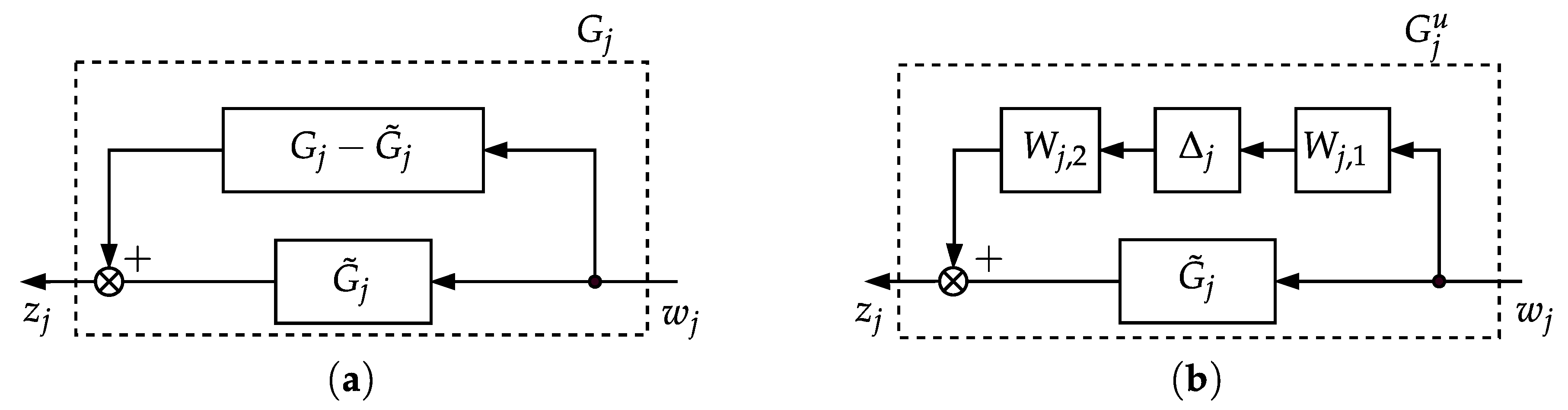
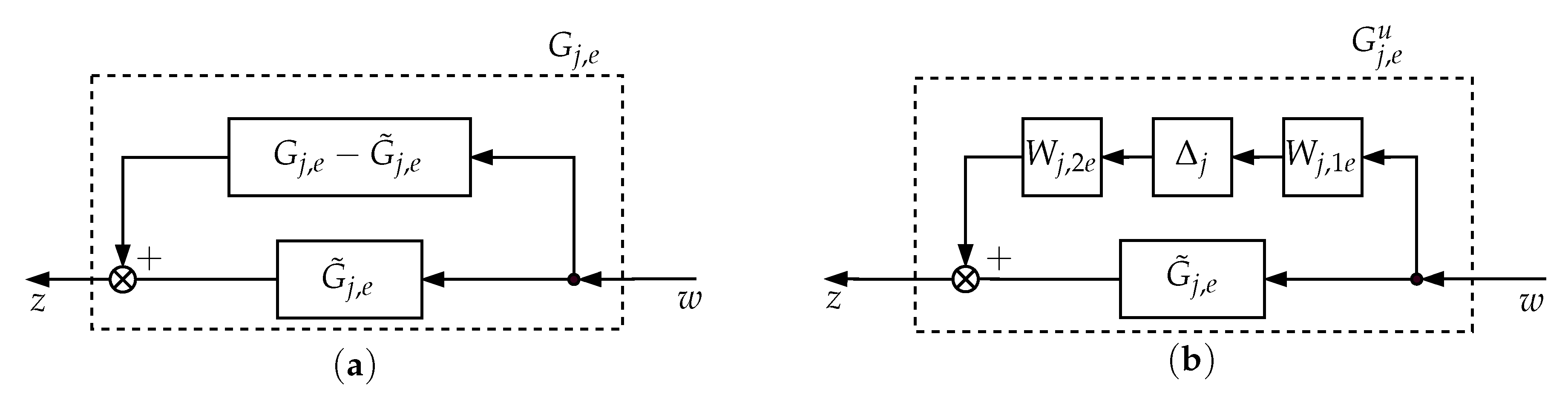
2.5. Additive Uncertainty Model

In order to capture the unknown effect that spatial discretization and MOR have on the resulting discretized and reduced order subsystems, the uncertainty is introduced. The type of uncertainty that is introduced into the analysis with spatial discretization and MOR can be considered as a modelling error [17,43]. This type of uncertainty can be modelled using input- or output-multiplicative uncertainty or additive uncertainty [17,37,43].

Due to the nature of the problem, having to model absolute gaps between the nominal and the uncertain model, and in order to preserve the structure of an interconnected system, an additive uncertainty model is used [43]. The absolute error between the original model and the reduced order discretized model can be calculated as $G_j-{\tilde{G}}_j$, and adding it back to the reduced order discretized model ${\tilde{G}}_j$, clearly results in a nominal model $G_j$. The absolute error and this type of addition is represented in Figure 1a.

The uncertainty can be introduced to the system as shown in Figure 1b. This uncertain system can be written by replacing the absolute error $G_j-\widetilde{G_j}$ with an appropriate uncertainty model as

$$G_j^u=\widetilde{G_j}+W_{j,2}{\Delta }_j{W}_{j,1},$$

(11)

where $G_j^u$ is the resulting uncertain subsystem, $\widetilde{G_j}$ represents a discretized and/or reduced order subsystem, $W_{j,1}$ and $W_{j,2}$ are assumed to be stable frequency weights, and ${∥{\Delta }_j∥}_{{\mathcal{H}}_{\infty }}\le 1$ is the uncertainty.

Let us now consider the system represented as in Figure 2. The frequency weights $W_{j,1}$ and $W_{j,2}$ can be incorporated into the nominal system, and together with the nominal part of the system are now defined as $\mathsf{\Gamma }$. This augmentation, shown in Figure 2, can be performed with linear fractional transformation (LFT) as

$$\left[\begin{array}{c}q\\ z\end{array}\right]=\underset{\mathsf{\Gamma }}{\underbrace{\left[\begin{array}{cc}{\mathsf{\Gamma }}_{qp}& {\mathsf{\Gamma }}_{qw}\\ {\mathsf{\Gamma }}_{zp}& {\mathsf{\Gamma }}_{zw}\end{array}\right]}}\left[\begin{array}{c}p\\ w\end{array}\right],p=\Delta \left(q\right),$$

(12)

which is often denoted using the Redheffer star product [43], or the ⋆ operator, as $z=(\Delta \star \mathsf{\Gamma })w$, where

$$\Delta \star \mathsf{\Gamma }:={\mathsf{\Gamma }}_{zw}+{\mathsf{\Gamma }}_{zp}\Delta {\left(I-{\mathsf{\Gamma }}_{qp}\Delta \right)}^{-1}{\mathsf{\Gamma }}_{qw},$$

and which is assumed to be well-posed for all $\Delta \in \mathsf{\Delta }$, where $\mathsf{\Delta }$ represents some set in which $\Delta$ can take values, that identifies the nature and structure of uncertainties (for more details see Section 2.6 and [25]). Here $\mathsf{\Gamma }\in {\mathcal{RH}}_{\infty }$ is a stable LTI system where $p\to q$ represents the uncertainty channel and $w\to z$ represents the performance channel.

With simple rearranging of the terms represented in Equation (11), and rewriting it as Equation (12), the expression for the LFT of an uncertain system with additive uncertainty reads as

$$\left[\begin{array}{c}{q}_j\\ z_j\end{array}\right]=\left[\begin{array}{cc}0& W_{j,1}\\ W_{j,2}& {\tilde{G}}_j\end{array}\right]\left[\begin{array}{c}{p}_j\\ w_j\end{array}\right].$$

(13)

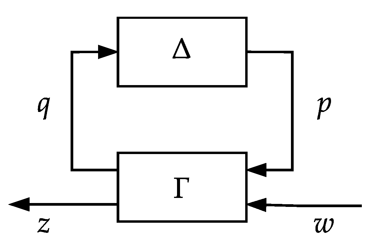
2.6. Robustness Analysis Using Integral Quadratic Constraints

Integral quadratic constraints (IQC) [24] represents an established unifying framework for the analysis of both robust stability and robust performance of uncertain systems. IQC essentially allow the analysis of a rich class of uncertainties by detaching the uncertainty $\Delta$ from the nominal part $\mathsf{\Gamma }$. The IQC analysis can be carried out without the explicit knowledge of the uncertainty $\Delta$ but rather with limited overall information of the energy transfer concerning its input-output properties. As shown in [24], this usually applies to a much larger set of uncertain operators that belong to a certain class $\mathsf{\Delta }$. The IQC analysis can be carried out in the frequency domain by finding solutions to frequency domain inequality (FDI) on a fixed grid of finite frequencies (thus making this semi-infinite problem). It was proven that this FDI can be turned into a finite convex feasibility problem with suitably parametrizing the multipliers [17,18,19,25]. After applying the so called Kalman–Yakubovich–Popov (KYP) lemma, the IQC problem can also be analysed in time domain [17,18,19,25]. A summary in details of steps required to transform this rather abstract concept into a computationally tractable problem can be found in [25], while here only some key points will be outlined. To illustrate this concept, we will examine the system as shown in Figure 2. First, we study the behaviour on the channel $p\to q$ representing the uncertainty channel.

Two signals $p\in {\mathcal{L}}_2$ and $q\in {\mathcal{L}}_2$ are said to satisfy the IQC defined by the multiplier $\mathsf{\Pi }$ [25] if

$$\mathcal{I}(\mathsf{\Pi },q,p):=〈\left(\begin{array}{c}q\\ p\end{array}\right),\left(\begin{array}{cc}{\mathsf{\Pi }}_{11}& {\mathsf{\Pi }}_{12}\\ {\mathsf{\Pi }}_{12}^{*}& {\mathsf{\Pi }}_{22}\end{array}\right)\left(\begin{array}{c}q\\ p\end{array}\right)〉\ge 0,$$

(14)

where $\mathsf{\Pi }$ is said to satisfy $\mathsf{\Pi }={\mathsf{\Pi }}^{*}\in {\mathcal{RL}}_{\infty }$. With $p=\Delta \left(q\right)$ IQC now reads

$$\mathcal{I}(\mathsf{\Pi },q,\Delta \left(q\right))\ge 0\forall q\in {\mathcal{L}}_2$$

(15)

it becomes possible to capture useful properties of uncertainties $\Delta \in \mathsf{\Delta }$ and describe its input-output energy transfer relations. In order to carry out a practical robust stability analysis, it is usual to construct a whole family of multipliers $\mathsf{\Pi }\subset {\mathcal{RL}}_{\infty }$ such that Equation (14) holds for all $\mathsf{\Pi }\in \mathsf{\Pi }\subset {\mathcal{RL}}_{\infty }$ and for all $\Delta \in \mathsf{\Delta }$.

In complete analogy, let us also examine the behaviour of the channel $w\to z$ on which we want to impose certain performance criteria, such that two signals signals $w\in {\mathcal{L}}_2$ and $z\in {\mathcal{L}}_2$ are said to satisfy the IQC defined by the multiplier ${\mathsf{\Pi }}_p$ [25] if

$${\mathcal{I}}_p({\mathsf{\Pi }}_p,z,w):=〈\left(\begin{array}{c}z\\ w\end{array}\right),\left(\begin{array}{cc}{\mathsf{\Pi }}_{p11}& {\mathsf{\Pi }}_{p12}\\ {\mathsf{\Pi }}_{p12}^{*}& {\mathsf{\Pi }}_{p22}\end{array}\right)\left(\begin{array}{c}z\\ w\end{array}\right)〉\ge -ϵ{∥w∥}^2,$$

(16)

where $ϵ>0$ is used to capture strict a version of the imposed performance specification. In order to carry out a practical robust performance analysis, it is usual to construct a whole family of multipliers ${\mathsf{\Pi }}_p\subset {\mathcal{RL}}_{\infty }$ such that Equation (16) holds for all ${\mathsf{\Pi }}_p\in {\mathsf{\Pi }}_p\subset {\mathcal{RL}}_{\infty }$, while the ${\mathsf{\Pi }}_p$ is confined to the set

$${\mathsf{\Pi }}_p\subset \left\{{\mathsf{\Pi }}_p\in {\mathcal{RL}}_{\infty }:{\mathsf{\Pi }}_{p11}\succcurlyeq 0\right\}$$

where the ${\mathsf{\Pi }}_{p11}\succcurlyeq 0$ is required in order to perform robust stability and performance at the same time, which we will often call just robustness analysis [25].

Besides tackling both robust stability and robust performance at the same time, another useful aspect of the IQC framework advantage is the possibility to perform robust stability of the interconnected systems where each of the subsystem can be affected by multiple uncertainties. A standard IQC framework can be expanded relatively with $\mathsf{\Gamma }$ and $\Delta$ being

$$\left(\begin{array}{cc}{\mathsf{\Gamma }}_{qp}& {\mathsf{\Gamma }}_{qw}\\ {\mathsf{\Gamma }}_{zp}& {\mathsf{\Gamma }}_{zw}\end{array}\right):=\left(\begin{array}{cccc}{\mathsf{\Gamma }}_{q_1{p}_1}& \cdots & {\mathsf{\Gamma }}_{q_1{p}_k}& {\mathsf{\Gamma }}_{q_{1}w}\\ ⋮& \ddots & ⋮& ⋮\\ {\mathsf{\Gamma }}_{q_k{p}_1}& \cdots & {\mathsf{\Gamma }}_{q_k{p}_k}& {\mathsf{\Gamma }}_{q_{k}w}\\ {\mathsf{\Gamma }}_{z{p}_1}& \cdots & {\mathsf{\Gamma }}_{z{p}_k}& {\mathsf{\Gamma }}_{zw}\end{array}\right)$$

(17)

and

$$\Delta \left(q\right):=\mathrm{col}\left({\Delta }_1\left(q_1\right),\cdots ,{\Delta }_k\left(q_k\right)\right)$$

(18)

where subsystems $j=1,\cdots ,k$ have linear fractional dependency on ${\Delta }_1,\cdots ,{\Delta }_k$ and ${\Delta }_j$ take their values in the sets ${\mathsf{\Delta }}_j$ [25]. Then Equation (2) needs to be well-posed for all ${\Delta }_j\in {\mathsf{\Delta }}_j$, where individual ${\Delta }_i$ blocks satisfy the IQC $\mathcal{I}({\mathsf{\Pi }}_i,q_i,{\Delta }_i\left(q_i\right))\ge 0,\forall q_i\in {\mathcal{L}}_2$, but also the composite IQC $\mathcal{I}(\mathsf{\Pi },q,\Delta \left(q\right))\ge 0,\forall q\in {\mathcal{L}}_2$ holds, with $q:=col\left(q_1,\cdots ,q_k\right)$ and

$$\mathsf{\Pi }=\left(\begin{array}{cc}\mathrm{diag}({\mathsf{\Pi }}_{1,11},\cdots {\mathsf{\Pi }}_{k,11})& \mathrm{diag}({\mathsf{\Pi }}_{1,12},\cdots {\mathsf{\Pi }}_{k,12})\\ \mathrm{diag}({\mathsf{\Pi }}_{1,12}^{*},\cdots {\mathsf{\Pi }}_{k,12}^{*})& \mathrm{diag}({\mathsf{\Pi }}_{1,22},\cdots {\mathsf{\Pi }}_{k,22})\end{array}\right).$$

Let us now state the central theorem, through a frequency domain inequality, as obtained in [24]. In all the FDIs we will use short notation where $G=G\left(i\omega \right)$, $\mathsf{\Pi }=\mathsf{\Pi }\left(i\omega \right)$ and ${\mathsf{\Pi }}_p={\mathsf{\Pi }}_p\left(i\omega \right)$.

Theorem 1.

Assume that

1.

for all $\tau \in [0,1]$ the interconnection defined with Equation (12), with omitted performance channels w and z, is well posed for $\mathsf{\Delta }$ replaced by $\tau \Delta$;

2.

for all $\tau \in [0,1]$ and some $\mathsf{\Pi }={\mathsf{\Pi }}^{*}\in {\mathcal{RL}}_{\infty }$, the IQC defined with Equation (14) is satisfied for $\mathsf{\Delta }$ replaced by $\tau \Delta$;

3.

the following FDI is satisfied:

$${\left(\begin{array}{c}\mathsf{\Gamma }\\ I\end{array}\right)}^{*}\mathsf{\Pi }\left(\begin{array}{c}\mathsf{\Gamma }\\ I\end{array}\right)\prec 0\forall \omega \in \mathbb{R}\cup \left\{\infty \right\}.$$

(19)

Then the interconnection defined by Equation (12), with omitted performance channels w and z, is stable.

With that in mind, the IQC for robustness analysis can be represented through a FDI as outlined in [25] which is an extension of Theorem 1.

Corollary 1.

Assume that

1.

for all $\Delta \in \mathsf{\Delta }$ the interconnection defined by Equation (12), with omitted performance channels w and z, is well posed;

2.

for all $\Delta \in \mathsf{\Delta }$ and for all $\mathsf{\Pi }\in \mathsf{\Pi }$ the IQC defined by Equation (14) is satisfied.

Then the interconnection defined with Equation (12) is robustly stable and robust performance on the channel $w\to z$ is guaranteed if there exists a $\mathsf{\Pi }\in \mathsf{\Pi }$ and ${\mathsf{\Pi }}_p\in {\mathsf{\Pi }}_p$ such that

$${\left(\begin{array}{cc}{\mathsf{\Gamma }}_{qp}& {\mathsf{\Gamma }}_{qw}\\ I& 0\\ {\mathsf{\Gamma }}_{zp}& {\mathsf{\Gamma }}_{zw}\\ 0& I\end{array}\right)}^{*}\left(\begin{array}{cc}\mathsf{\Pi }& 0\\ 0& {\mathsf{\Pi }}_p\end{array}\right)\left(\begin{array}{cc}{\mathsf{\Gamma }}_{qp}& {\mathsf{\Gamma }}_{qw}\\ I& 0\\ {\mathsf{\Gamma }}_{zp}& {\mathsf{\Gamma }}_{zw}\\ 0& I\end{array}\right)\prec 0.$$

(20)

The proof can be found in Appendix A in [25]. Robustness analysis, according to Corollary 1, simply boils down to checking if there exists a $\mathsf{\Pi }\in \mathsf{\Pi }$ and ${\mathsf{\Pi }}_p\in {\mathsf{\Pi }}_p$ such that FDI defined with Equation (19) holds true, under the assumptions that both conditions in Corollary 1 are met. If so, then the robust performance is achieved and the uncertain system is robustly stable.

To render the presented IQC framework for robustness analysis computationally tractable, a suitable parametrization of $\mathsf{\Pi }$ and ${\mathsf{\Pi }}_p$ is required, such that Equation (20) results in a linear constraint on some set of unknown variables [18,25]. This can be achieved if the families of multipliers are parametrized as

$$\begin{array}{cc}\hfill \mathsf{\Pi }& =\left\{{\mathsf{\Psi }}^{*}P\mathsf{\Psi }:P\in \mathit{P}\right\},\hfill \end{array}$$

(21)

$$\begin{array}{cc}\hfill {\mathsf{\Pi }}_p& =\left\{{\mathsf{\Psi }}_p^{*}{P}_p{\mathsf{\Psi }}_p:P_p\in {\mathit{P}}_p\right\},\hfill \end{array}$$

(22)

with an LMIable sets $\mathit{P}$ and ${\mathit{P}}_p$ of real symmetric matrices $P\in \mathbb{S}$ and $P_p\in \mathbb{S}$, respectively, and some fixed and typically tall transfer matrices $\mathsf{\Psi }\in {\mathcal{RH}}_{\infty }$ and ${\mathsf{\Psi }}_p\in {\mathcal{RH}}_{\infty }$. A set is LMIable if it can be represented as the feasible set of an LMI constraint [17,38]. Now the robustness analysis can be characterized as follows.

Corollary 2.

Assume that

1.

for all $\Delta \in \mathsf{\Delta }$ the interconnection defined with Equation (12) is well posed;

2.

for all $\Delta \in \mathsf{\Delta }$ and for all $P\in \mathit{P}$ the IQC defined with Equation (14) is satisfied with $\mathsf{\Pi }={\mathsf{\Psi }}^{*}P\mathsf{\Psi }$.

Then the interconnection defined with Equation (12) is robustly stable and robust performance on the channel $w\to z$ is guaranteed if there exists a $P\in \mathit{P}$ and $P_p\in {\mathit{P}}_p$ such that

$${\left(\begin{array}{cc}{\mathsf{\Gamma }}_{qp}& {\mathsf{\Gamma }}_{qw}\\ I& 0\\ {\mathsf{\Gamma }}_{zp}& {\mathsf{\Gamma }}_{zw}\\ 0& I\end{array}\right)}^{*}\left(\begin{array}{cc}{\mathsf{\Psi }}^{*}P\mathsf{\Psi }& 0\\ 0& {\mathsf{\Psi }}_p^{*}Pp{\mathsf{\Psi }}_p\end{array}\right)\left(\begin{array}{cc}{\mathsf{\Gamma }}_{qp}& {\mathsf{\Gamma }}_{qw}\\ I& 0\\ {\mathsf{\Gamma }}_{zp}& {\mathsf{\Gamma }}_{zw}\\ 0& I\end{array}\right)\prec 0.$$

(23)

The obtained FDI defined with Equation (23) is affine in the matrix variables P and $P_p$. Therefore, if both sets $\mathit{P}$ and ${\mathit{P}}_p$ are LMIable, we obtain a semi-infinite convex robustness analysis feasibility test of the system represented with Equation (12) [18,25]. This FDI needs to hold true for all $\omega \in \mathbb{R}\cup \left\{\infty \right\}$, or on the fixed grid of properly distributed frequencies. To avoid this, at the cost of the increased computation, it is possible to satisfy Equation (23) for all frequencies $\omega \in \mathbb{R}\cup \left\{\infty \right\}$ by using the Kalman–Yakubovich–Popov (KYP) lemma (often called positive-real and bounded-real lemma).

Lemma 1.

Let $P\in \mathbb{S}$ and let $\mathsf{\Gamma }\in {\mathcal{RL}}_{\infty }$ admit the realization $\left(A_{\mathsf{\Gamma }},B_{\mathsf{\Gamma }},C_{\mathsf{\Gamma }},D_{\mathsf{\Gamma }}\right)$ with $A_{\mathsf{\Gamma }}\in \mathbb{R}$ and $eig\left(A_{\mathsf{\Gamma }}\right)\cap {\mathbb{C}}^0=\varnothing$. The following two statements are equivalent:

1.

${\mathsf{\Gamma }}^{*}P\mathsf{\Gamma }\prec 0$.

2.

There exists a matrix $X\in \mathbb{S}$ such that

$${\left(\begin{array}{cc}I& 0\\ A_{\mathsf{\Gamma }}& B_{\mathsf{\Gamma }}\\ C_{\mathsf{\Gamma }}& D_{\mathsf{\Gamma }}\end{array}\right)}^T\left(\begin{array}{ccc}0& X& 0\\ X& 0& 0\\ 0& 0& P\end{array}\right)\left(\begin{array}{cc}I& 0\\ A_{\mathsf{\Gamma }}& B_{\mathsf{\Gamma }}\\ C_{\mathsf{\Gamma }}& D_{\mathsf{\Gamma }}\end{array}\right)\prec 0.$$

(24)

The corresponding equivalence persists to hold for

• non-strict inequalities, if, in addition, the pair $(A_{\mathsf{\Gamma }},B_{\mathsf{\Gamma }})$ is controllable,
• equalities, if, in addition, $A_{\mathsf{\Gamma }}$ is Hurwitz and the pair $(A_{\mathsf{\Gamma }},B_{\mathsf{\Gamma }})$ is controllable.

Proof and the details of the KYP lemma can be found in [17,18,25] and the references therein. Now the FDI defined with the Equation (23) can be checked numerically. For this purpose let us introduce the following realization

$$\left(\begin{array}{cc}\mathsf{\Psi }& 0\\ 0& {\mathsf{\Psi }}_p\end{array}\right)\left(\begin{array}{cc}{\mathsf{\Gamma }}_{qp}& {\mathsf{\Gamma }}_{qw}\\ I& 0\\ {\mathsf{\Gamma }}_{zp}& {\mathsf{\Gamma }}_{zw}\\ 0& I\end{array}\right)=\left(\begin{array}{ccc}{A}_R& B_{R1}& B_{R2}\\ C_{R1}& D_{R11}& D_{R11}\\ C_{R2}& D_{R21}& D_{R22}\end{array}\right)$$

(25)

where $A_R\in \mathbb{R}$, $\mathrm{eig}\left(A_R\right)\subset {\mathbb{C}}^{-}$, and state the following.

Corollary 3.

Assume that

1.

for all $\Delta \in \mathsf{\Delta }$ the interconnection defined by Equation (12) is well posed;

2.

for all $\Delta \in \mathsf{\Delta }$ and for all $P\in \mathit{P}$ the IQC defined by Equation (14) is satisfied with $\mathsf{\Pi }={\mathsf{\Psi }}^{*}P\mathsf{\Psi }.$ Then the interconnection defined with the Equation (12) is robustly stable and robust performance on the channel $w\to z$ is guaranteed, if there exist $X\in \mathbb{S}$, $P\in \mathit{P}$ and $P_p\in {\mathit{P}}_p$ such that

$${\left(\begin{array}{ccc}I& 0& 0\\ A_R& B_{R1}& B_{R2}\\ C_{R1}& D_{R11}& D_{R12}\\ C_{R2}& D_{R21}& D_{R22}\end{array}\right)}^T\left(\begin{array}{cccc}0& X& 0& 0\\ X& 0& 0& 0\\ 0& 0& P& 0\\ 0& 0& 0& P_p\end{array}\right)\left(\begin{array}{ccc}I& 0& 0\\ A_R& B_{R1}& B_{R2}\\ C_{R1}& D_{R11}& D_{R12}\\ C_{R2}& D_{R21}& D_{R22}\end{array}\right)\left(\begin{array}{cc}I& 0\\ A_{\mathsf{\Gamma }}& B_{\mathsf{\Gamma }}\\ C_{\mathsf{\Gamma }}& D_{\mathsf{\Gamma }}\end{array}\right)\prec 0.$$

(26)

Hence, if $\mathit{P}$ and ${\mathit{P}}_p$ are LMIable sets, a finite dimensional convex feasibility test for robustness analysis is obtained.

To complete the analysis via IQC, let us also formulate multiplier classes suitable for uncertainties dealt with in this paper as well as a multiplier class suitable for performance cost in this paper. Throughout the paper we will use a basis-function ${\psi }_v\in {\mathcal{RH}}_{\infty }^{(v+1)\times 1}$ that is fixed and has a McMillan degree of v, to obtain inner approximations (i.e., subsets) of the multipliers defined with the Equations (21) and (22), defined as

$${\psi }_v\left(i\omega \right):={\left(\begin{array}{ccccc}1& \frac{1}{(i\omega -\rho )}& \frac{1}{{(i\omega -\rho )}^2}& \cdots & \frac{1}{{(i\omega -\rho )}^v}\end{array}\right)}^T$$

(27)

with the minimal state-space realization

$${\psi }_v=\left(\begin{array}{c}\begin{array}{cc}{A}_v& B_v\\ C_v& D_v\end{array}\end{array}\right)=\left(\begin{array}{cccccc}\rho & 0& \cdots & \cdots & 0& 1\\ 1& \ddots & \ddots & \ddots & \cdots & 0\\ 0& \ddots & \ddots & \ddots & \cdots & ⋮\\ ⋮& \ddots & \ddots & \ddots & \cdots & ⋮\\ 0& \cdots & 0& 1& \rho & 0\\ \mathrm{}& \mathrm{}& 0& \mathrm{}& \mathrm{}& 1\\ \mathrm{}& \mathrm{}& I_v& \mathrm{}& \mathrm{}& 0\end{array}\right)$$

(28)

where $\rho <0$ represents the location of the pole and $v\in \mathbb{N}$. By changing $\rho$ over line search with for example $v\in \left\{1,2,3,4,5\right\}$ allows for dynamics in the multipliers and gives freedom in search for the feasible solution of Equation (26). This implies that the parametrization using such basis function is sufficiently rich to approximate general sets of multipliers. For other basis-functions that can be used, readers are referred to [25,26]).

Unstructured uncertainties as described in Section 2.5 belong to a class of an uncertain LTI dynamics for which it can be said that $\Delta$ is confined to a set of LTI dynamic full-block uncertainties

$${\mathsf{\Delta }}_{\mathrm{lti},\mathrm{dyn},\mathrm{fb}}:=\left\{\Delta \in {\mathcal{H}}_{\infty }:{∥\Delta ∥}_{\infty }\le 1\right\}.$$

(29)

Uncertainties of this form can be captured with the following multiplier class. For all the $\Delta \in {\mathsf{\Delta }}_{\mathrm{lti},\mathrm{dyn},\mathrm{fb}}$ the IQC (15) holds with

$${\mathsf{\Psi }}^{*}P\mathsf{\Psi }:={\left(\begin{array}{cc}{\psi }_v\otimes I& 0\\ 0& {\psi }_v\otimes I\end{array}\right)}^{*}\left(\begin{array}{cc}{P}_{11}\otimes I& 0\\ 0& -P_{11}\otimes I\end{array}\right)\left(\begin{array}{cc}{\psi }_v\otimes I& 0\\ 0& {\psi }_v\otimes I\end{array}\right),$$

(30)

if

$${\psi }_v^{*}{P}_{11}{\psi }_v\ge 0.$$

(31)

Here, $P_{11}\in {\mathbb{S}}^{v+1}$ is a free matrix variable and ${\psi }_v$ is a fixed basis-function as defined with Equation (27). By using the basis-function as defined with Equation (28) in its state-space form, we can infer that Equation (31) is equivalent to the existence of some matrix $X_v\in {\mathbb{S}}^v$ such that the following LMI holds true

$${\left(\begin{array}{cc}I& 0\\ A_v& B_v\\ C_v& D_v\end{array}\right)}^T\left(\begin{array}{ccc}0& X_v& 0\\ X_v& 0& 0\\ 0& 0& P_{11}\end{array}\right)\left(\begin{array}{cc}I& 0\\ A_v& B_v\\ C_v& D_v\end{array}\right)\succcurlyeq 0.$$

(32)

As it will be stated in the next chapter, we will also need a performance criterion on the channel $w\to z$ for the reduced order interconnected system to be kept as close as possible to the original (i.e., unreduced) interconnected system. The class of performance criteria, suitable for this matter, can be expressed in terms of induced ${\mathcal{L}}_2$-gain. Consider the stable system ${\mathsf{\Gamma }}_{zw}\in {\mathcal{RH}}_{\infty }$ and suppose there exists some $\gamma >0$ and some small $ϵ>0$ such that for all trajectories of $z={\mathsf{\Gamma }}_{zw}w$, with $w\in {\mathcal{L}}_2$, the performance IQC defined with Equation (16) is satisfied with

$${\mathsf{\Psi }}_p^{*}{P}_p{\mathsf{\Psi }}_p:=\left(\begin{array}{cc}I& 0\\ 0& I\end{array}\right)\left(\begin{array}{cc}{\gamma }^{-1}I& 0\\ 0& -\gamma I\end{array}\right)\left(\begin{array}{cc}I& 0\\ 0& I\end{array}\right).$$

(33)

Then the induced ${\mathcal{L}}_2$-gain from w to z is less than $\gamma >0$. Equation (33) can be linearised using Schur-complement [25]. In our case, we are interested in the best achievable induced ${\mathcal{L}}_2$-gain of the uncertain system defined with the Equation (2), while guaranteeing robust stability for all $\Delta \in {\Delta }_{\mathrm{lti},\mathrm{dyn},\mathrm{fb}}$. This can be achieved by applying Corollary 3 with Equations (30), (31) and (33).

3. Results

To model uncertainties for spatially discretized and reduced order spatially distributed dissipative dynamical systems that are suitable for (distributed) robust controller synthesis, an interconnected system consisting of many subsystems with as low-order and as least conservative uncertainties as possible, arising from both discretization and MOR, has to be obtained.

As seen from Equation (11) and the definition of ${\Delta }_j$ only being bounded by the ${\mathcal{H}}_{\infty }$-norm, this type of uncertainty is often called unstructured uncertainty. With this in mind, the uncertainty modelling essentially boils down to choosing the appropriate weights that essentially adjust (or scale) the amount of required uncertainty at each frequency. In practice, the weights are usually some combination of low-pass, band-pass and high-pass filters [17,43]. Indeed, as it is recognized in the literature, modelling of appropriate weighting filters (in general) is perhaps one of the most important jobs of a system engineer [44]: “…design of a robust and high-performance control system relies heavily on the choice of weights used in the design…”. Modelling the frequency weights, allows the control designer to capture the system uncertainties and to determine over what frequency ranges the performance is desired. Weights can be viewed as a way to fine tune the control design to achieve a desired level of performance and robustness without having to explicitly consider the system stability [45].

The authors stress that the uncertainty conservatism reduction method presented so far is essentially local. As it will be shown in the sequel, uncertainties modelled with structure preservation in mind can be further improved, thus, the subsystem uncertainty conservatism can be further reduced. Due to the mutual interconnections of the subsystems, and the fact that the subsystems and/or interconnections are dissipative, part of the uncertainty (especially in the high frequency range) can be discarded. The theoretical part regarding the definition of dissipative systems can be found in [17], while the simple explanation can be given in terms of energy loss throughout the system. The idea is to reduce the uncertainty conservatism of each subsystem, thus reducing the conservatism of the overall interconnected system as well, by studying energy losses throughout the system. However, in the meantime, it is also important to keep the order of the interconnected system as low as possible. While doing both of these things, the following mandatory things need to be achieved: (i) the reduced order discretized interconnected subsystem needs to be robustly stable; (ii) the order of the interconnected system should be kept as low as possible and; (iii) robust performance of the reduced order discretized interconnected system needs to be as close as possible to the performance of the reference interconnected system. To achieve the points stated previously, we propose a novel design procedure that is explained in the next section.

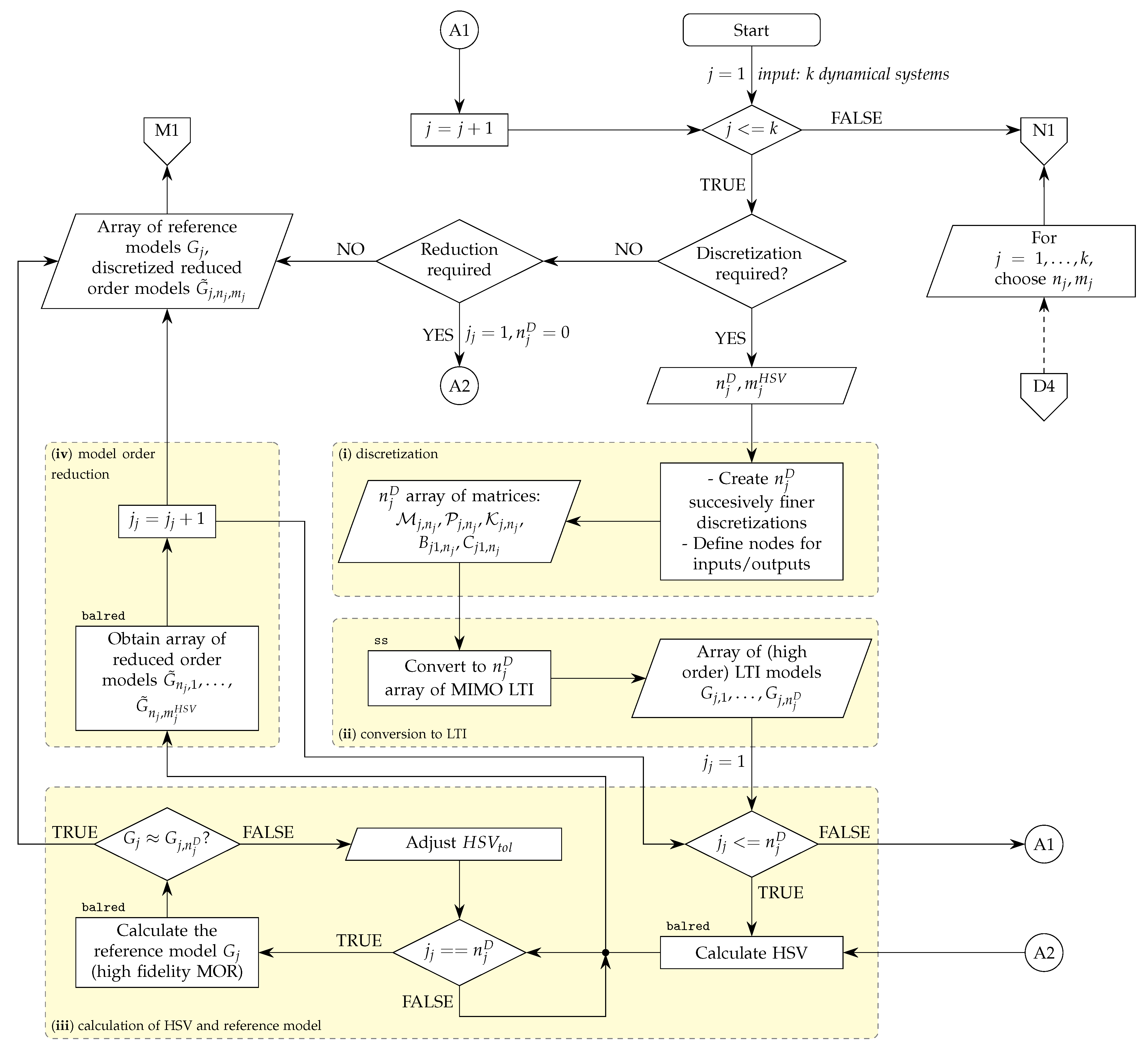
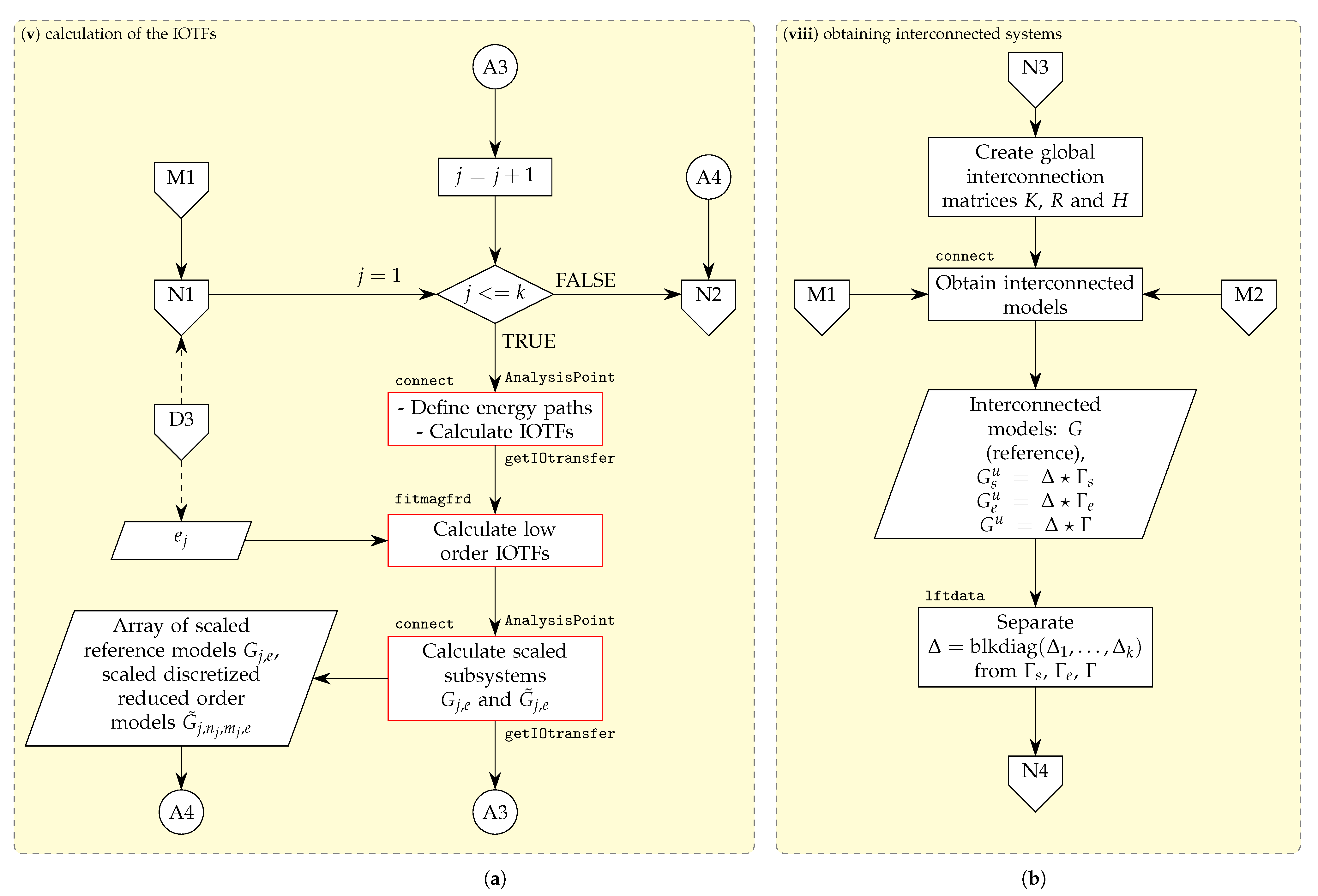
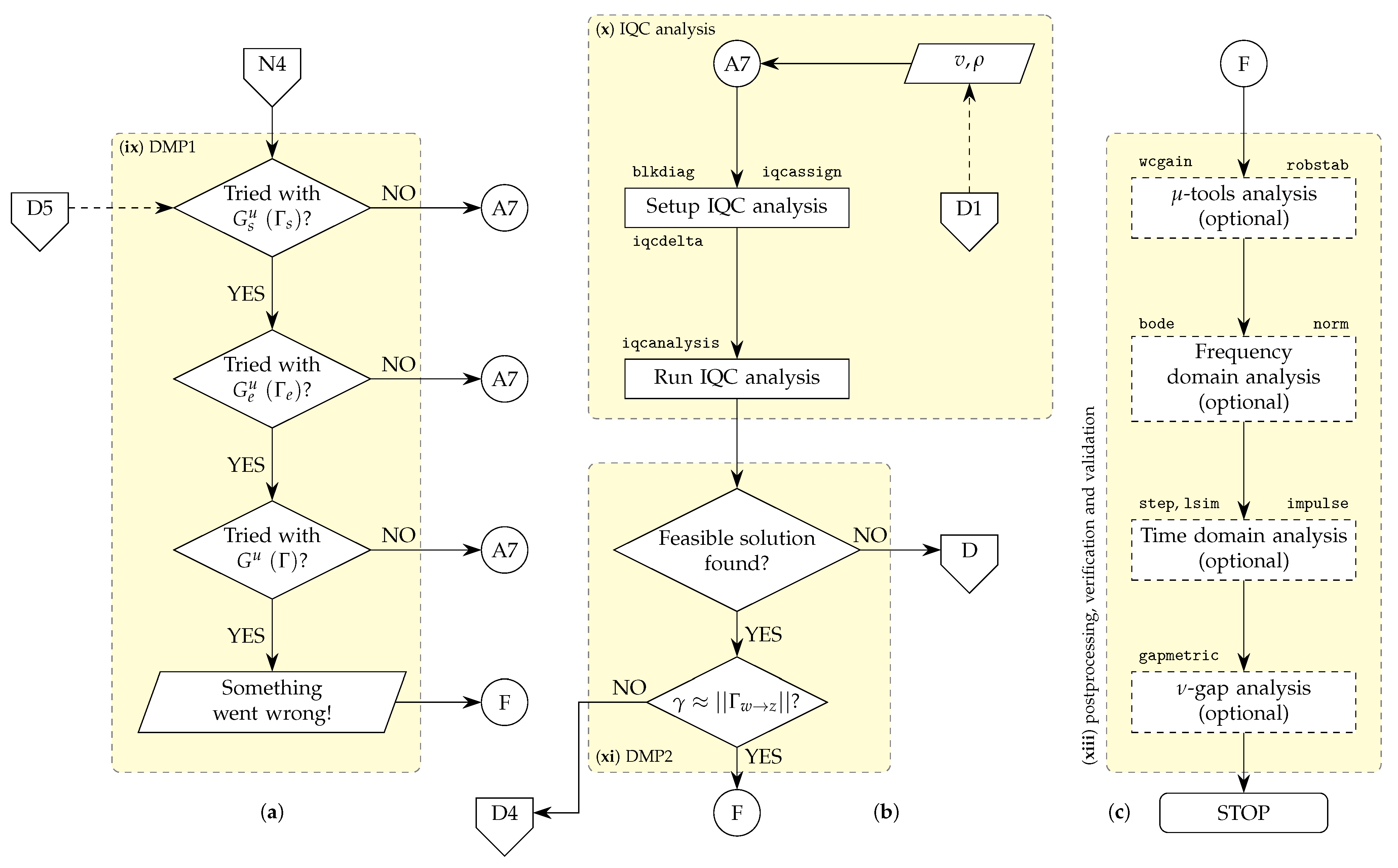
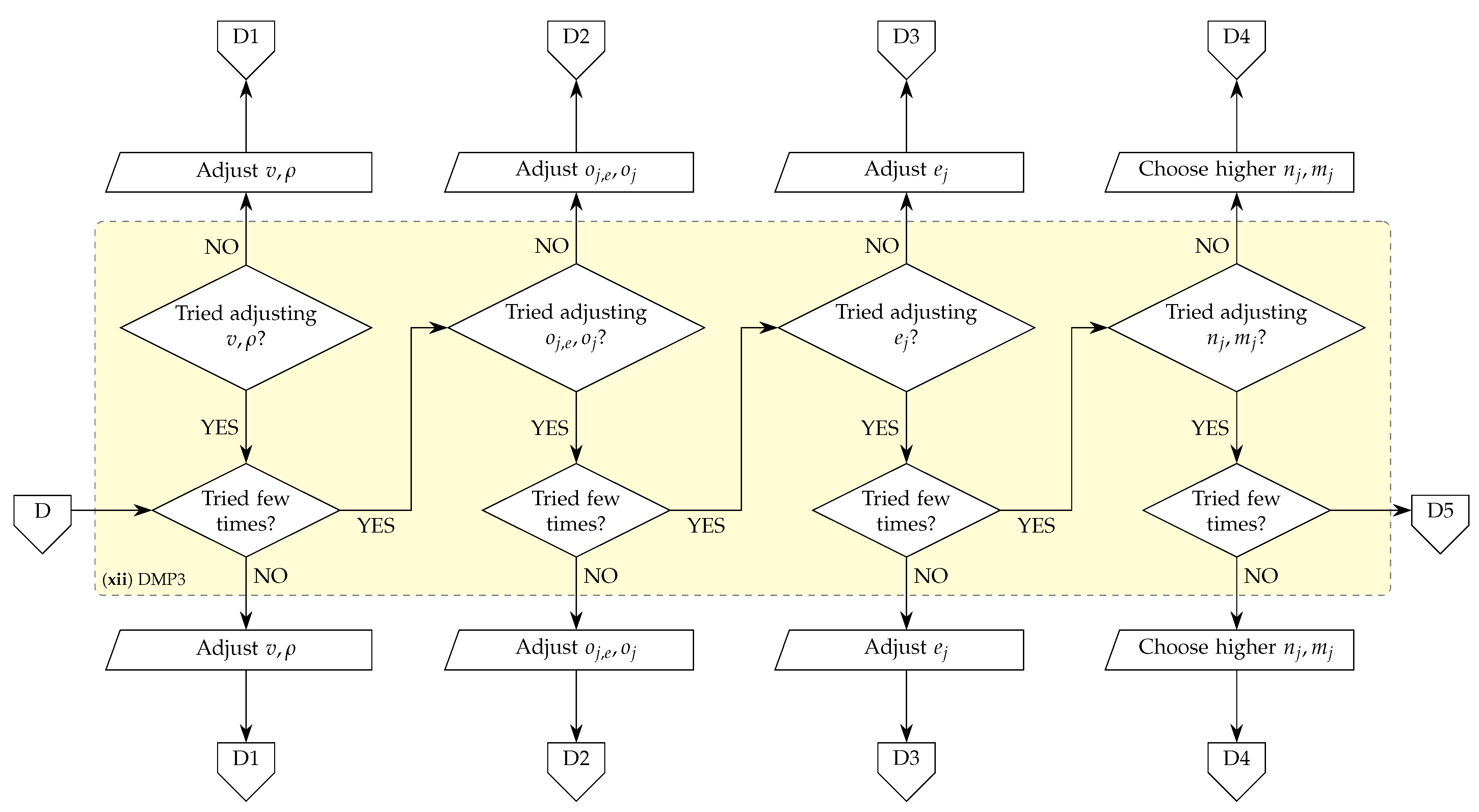
3.1. Design Procedure

The newly developed deign procedure will be written out as ready to implement in MATLAB philosophy, so wherever appropriate, useful MATLAB commands and routines will be highlighted. For the complete usage and compatibility, latest (as of date of article publishing) version of MATLAB, Control system toolbox™ and Robust control toolbox™ should be used. In the IQC robustness analysis part of the procedure, commands from the IQCLab Toolbox (V3.0) [26] are also mentioned.

To calculate the absolute error and additive uncertainty, an array of models is created. Reference models $G_j$ are obtained from the finest discretization. The discretized reduced order models are distinguished by the discretization using index $n_j=1,\cdots ,n_j^D$ and the order (states kept) using index $m_j=1,\cdots ,m_j^{HSV}$. For simplicity we will often omit these indexes and just write ${\tilde{G}}_j:={\tilde{G}}_{j,n_j,m_j}$. This process of obtaining an array of reference and discretized reduced order models is shown in Figure 3 and represented with steps (i) to (iv) therein.

We continue by choosing appropriate discretizations ($n_j$) and orders ($m_j$) of reduced order models for each subsystem. After that, the idea is to scale both the reference model and the discretized reduced order model to obtain a scaled version of the absolute error denoted as $G_{j,e}-{\tilde{G}}_{j,e}$ for each subsystem. We stress that these scalings can be directly calculated from the structure of the system and the fact that the subsystems are dissipating energy will be potentially beneficial—we will call these scalings input-output transfer functions (IOTFs) and details on how to obtain these are detailed later in Section 4.2 and Section 4.3. This process is shown in Figure 4 and denoted as a step (v). Besides the novelty of the overall procedure—or the approach to the discretization and model order reduction error uncertainty modelling—this step (i.e., (v)) also represents a first major novelty of the procedure. The fact that using only the existing structure of the system it is possible to reduce the uncertainty conservatism is something not yet seen.

With scalings (IOTFs) calculated, a scaled version of the absolute error, $G_{j,e}-{\tilde{G}}_{j,e}$, can be calculated for each subsystem. Due to the dissipative nature of the interconnected system, some of the energy is lost when coming to and from each subsystem, such that if we compared the gain of $G_{j,e}-{\tilde{G}}_{j,e}$ in comparison to the unscaled version of it, i.e., $G_j-{\tilde{G}}_j$, a significantly lower gain over a wide frequency range can be observed. As stated before, the main idea of additive uncertainty modelling is to replace these errors with the appropriate frequency weights—thus we introduce weights $W_{j,1e}$ and $W_{j,1}$ to capture the dynamic behaviour of the aforementioned errors. Steps for obtaining the uncertainty weights, a scaled version and an unscaled version, for each subsystem, are shown in Figure 5 denoted with (vi) and (vii), respectively. The second main novel part if being two fold. First, by observing the dynamic behaviour, of the scaled absolute error particularly, and to a lesser degree of the unscaled absolute error as well—there usually are no high peaks in gain. As such, it makes sense to use the weights of low order to capture such a behaviour. This can efficiently be obtained using low order logarithmic-Chebyshev magnitude filter design—the details on this particular choice of filter are elaborated in Section 4.1. The second part of the second major novelty comes from the observation, that in many cases, one can completely reduce the order of the filter—by simply choosing a filter of static (constant) gain—thus no additional states are introduced in the model at increase in conservatism.

Since this fact (of not increasing the order of the uncertain system) comes with practical usability, from now on, we will focus mostly on these weights, i.e., $W_{j,1s}$, to a lesser degree on the scaled (refined) weights $W_{j,1e}$ and only keep in mind the unscaled (unrefined) weights $W_{j,1}$ that are overly conservative when we do a comparison to demonstrate the results (for details see on a practical example in Section 3.2). All the dynamic behaviour will be captured only by weights $W_{j,1s}$ (or $W_{j,1e}$ or $W_{j,1}$), while the second weight will be kept to be identity. A more elaborate description on when one might use $W_{j,2}$ is given in Section 4.4. Moreover, ${\Delta }_j$ per subsystem always stays the same. With that being said, an array of uncertain subsystems can be created.

With the arrays of reference models and uncertain systems ready, as shown in Figure 4, denoted as a process (vii), we can obtain interconnected models. Here it should be noted that interconnection matrices R, K and H can be reused to calculate reference interconnected system G (used only for comparison and verification) and uncertain interconnected system(s). Again, we will keep our attention at the uncertain interconnected system $G_{j,s}^u$, while the other uncertain system $G_{j,e}^u$ can have practical usage, the uncertain system $G_j^u$ is only used to demonstrate the effect of uncertainty conservatism reduction (often called uncertainty refinement).

The last step of the process is to carry out robustness analysis. In this paper, we focus on the robustness analysis using integral quadratic constrains (IQCs). Without going into details (which are given in Section 2.6), the key point can be explained as follows. For a given interconnected uncertain system (previously converted to a LFT form)—again, focus is on $G_{j,s}^u$)—find a feasible solution to prove that the given uncertain system is robustly stable. After that, check the best achievable $\gamma$ and compare it to the induced ${\mathcal{L}}_2$-gain of a reference interconnected system. This part of the procedure is shown in Figure 6 and denoted as (x).

It should be noted that since the proposed procedure deals with the uncertainty modelling (or modelling in general), many parts of the process require manual operation. For example, the initial guess of the required discretization and/or orders of reduced order models (i.e., $n_j$ and $m_j$, respectively) a feasible solution might be found immediately and the performance criteria met easily. On the other hand, it might be a complete miss. Here, however, a main paradigm when choosing discretization and orders is to model systems close to the external inputs and outputs with relatively fine discretization and relatively high orders; and the one far away with coarse mesh and low orders. This also intuitively makes sense to do, since the dynamics of the distant subsystems is not affected by the external inputs or does not influence the measured outputs. With that being said, we complete the design procedure by proposing a useful decision making process (DMP), as shown in Figure 7, that can be used to efficiently find an uncertain interconnected system for which a robustness will be guaranteed.

Authors stress that carrying out robustness analysis using $\mu$-tools instead of IQC analysis is as easy as reformulating questions in the decision making process of the IQCs analysis (see (xi) DMP2 in Figure 6)—where “Feasible solution found?” becomes “Robust stability margin greater then 1?”| and “$\gamma \approx \left|\right|{\mathsf{\Gamma }}_{w\to z}\left|\right|$?” becomes “Worst case gain close to $\left|\right|{\mathsf{\Gamma }}_{w\to z}\left|\right|$?”.

One more note will be given before proceeding to the numerical example. While in the proposed design procedure we exclusively used either static $W_{j,1s}$ or refined $W_{j,1e}$ weights to obtain the uncertain interconnected system—an important advantage of the structure preserving approach is that one can combine static and refined weights per each subsystem (i.e., some subsystems’ uncertainty is modelled using static weights and for some other using refined weights). This gives the opportunity to further fine tune a trade-of between reduction in the uncertainty conservatism and the order of the interconnected uncertain system. It is left to the interested readers as a mental exercise to see how this can be utilised properly for a specific problem—because the modelling of each new complex interconnected dynamical system is a problem for itself.

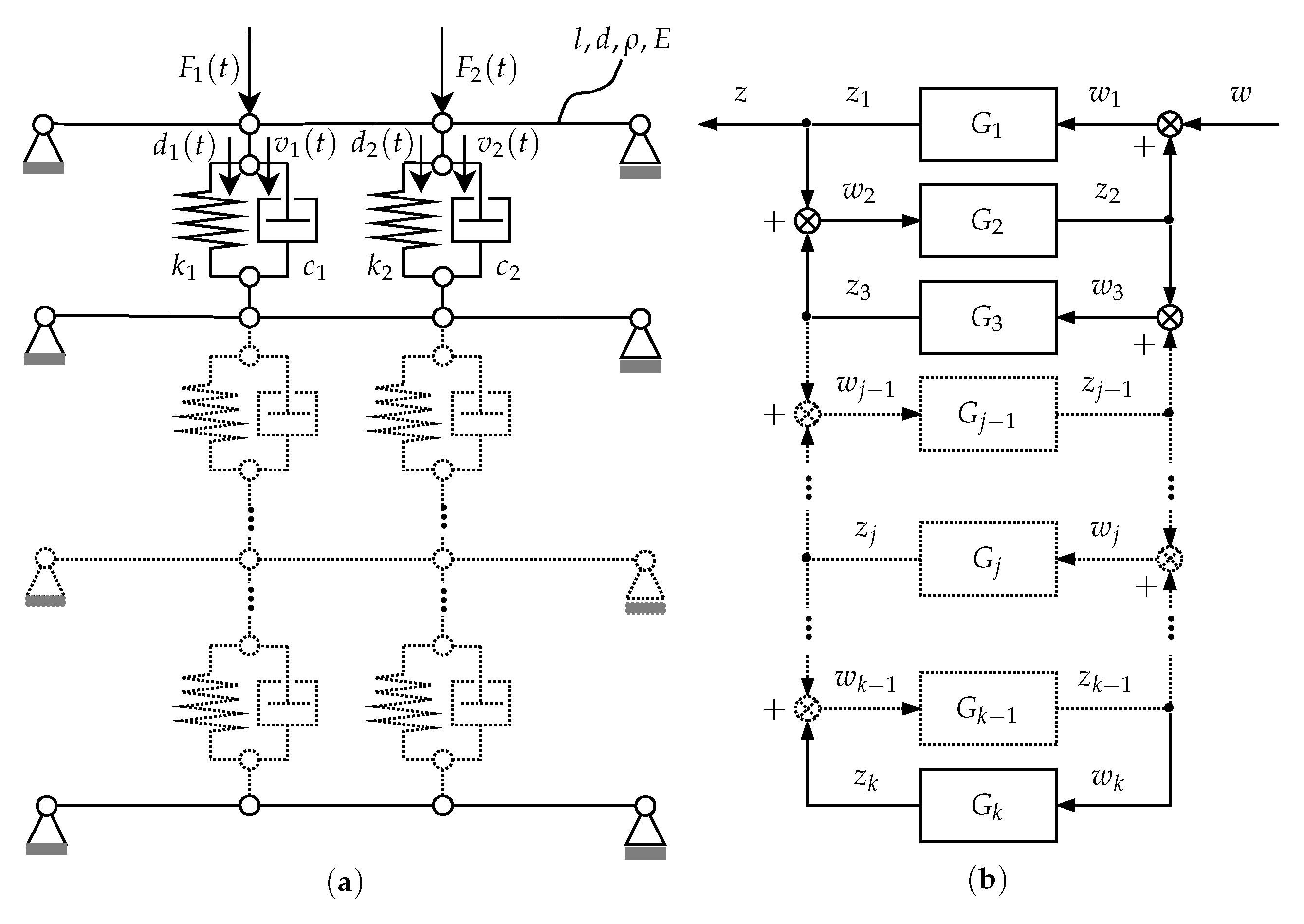
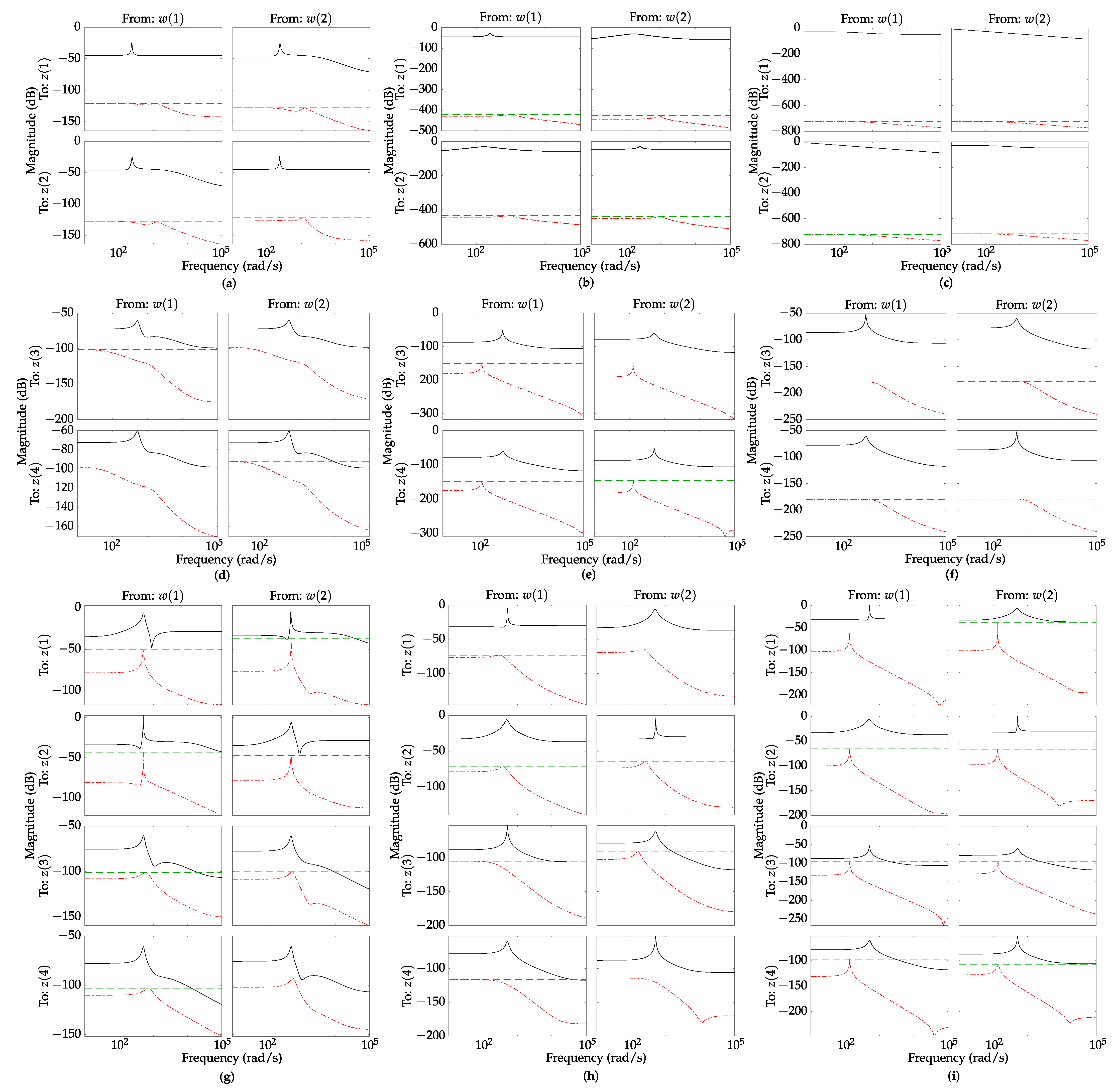
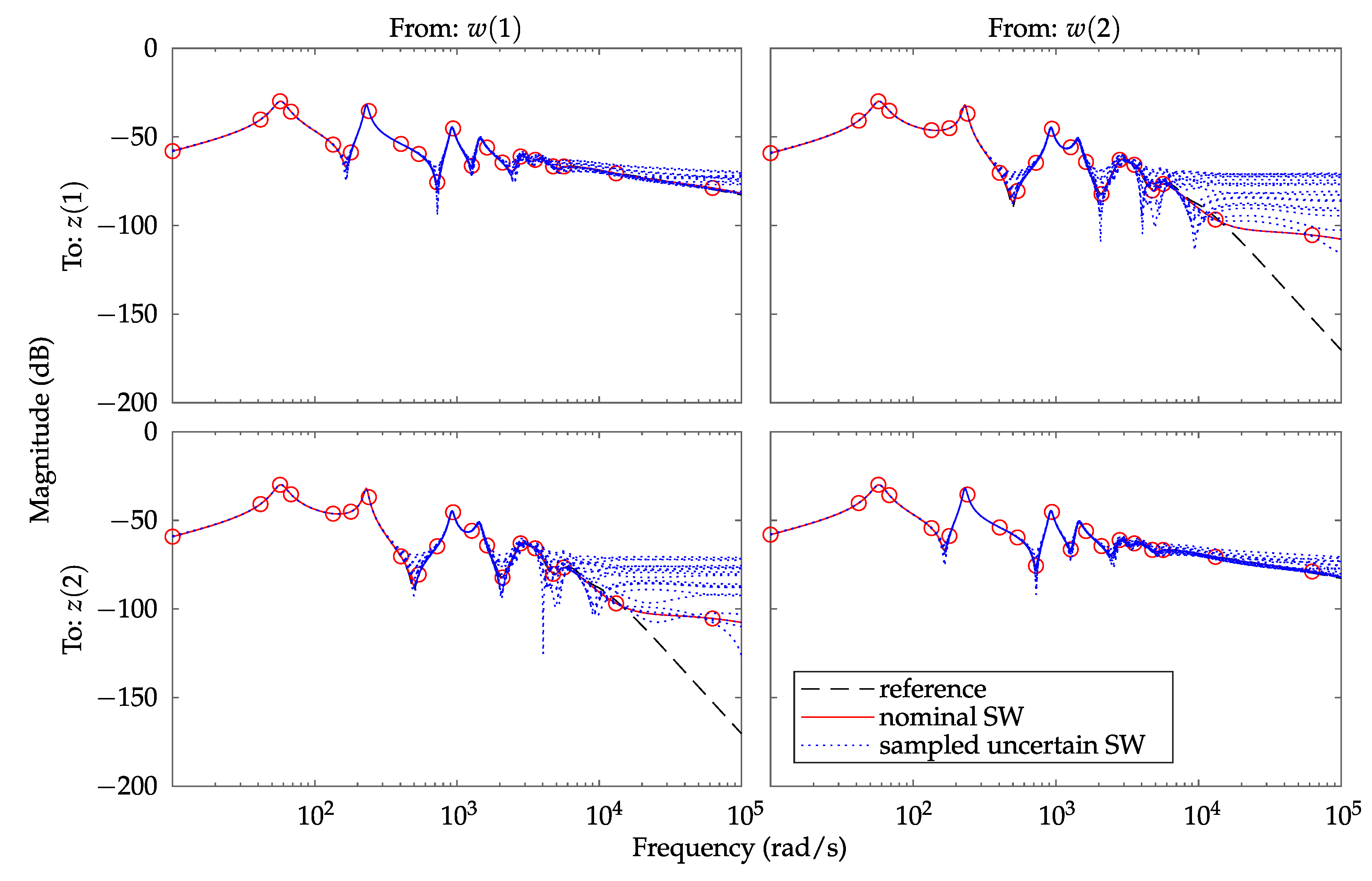
3.2. Numerical Example: Series of Simply Supported Euler Beams Mutually Interconnected by Springs and Dampers

All the code needed to replicate the results shown in the sequel is available in GitHub [46] and archived in Zenodo [47].

Let us now consider the application of the proposed procedure on the practical example—a series of simply supported Euler beams mutually interconnected by springs and dampers. Such a system is shown in Figure 8a. All beams of equal length l, divided into three ($n_s=3$) equal length segments, the same circular cross section with diameter of d, the same mass density $\rho$ and the same Young’s modulus of elasticity E. On the uppermost beam, at one third and two thirds of its length, two dynamical vertical forces $F_1\left(t\right)$ and $F_2\left(t\right)$ are applied. At the same locations, displacements of the beam $d_1\left(t\right)$ and $d_2\left(t\right)$, and velocities $v_1\left(t\right)$ and $v_2\left(t\right)$, respectively, are measured. On those same locations, spring-damper pairs are connected to the next successive beam. Internal inputs to the beams are forces acting from spring and dampers to the nodes at the beams, while the internal outputs are displacements and velocities of nodes at beams. Material properties of the beams, as well as stiffnesses of the springs and viscous damping coefficient of the dampers, are shown in

Table 1. Material properties of the beams, springs and dampers.

Case	l	d	$\mathit{\rho }$	E	${\mathit{c}}_1$	${\mathit{k}}_1$	${\mathit{c}}_2$	${\mathit{k}}_2$	$\mathit{\zeta }$
#	$\mathbf{m}$	${\mathbf{m}}^{\mathbf{2}}$	$\mathbf{kg}/{\mathbf{m}}^{\mathbf{3}}$	$\mathbf{GPa}$	$\mathbf{N}·\mathbf{s}/\mathbf{m}$	$\mathbf{N}·\mathbf{s}/\mathbf{m}$	$\mathbf{N}/\mathbf{m}$	$\mathbf{N}/\mathbf{m}$	-
1	2	$0.018$	7800	210 × ${10}^9$	${10}^{-4}$	0	${10}^{-6}$	0	$0.08$
2	2	$0.01$	7800	$210\times {10}^9$	0	$7\times {10}^0$	0	$3\times {10}^1$	$0.08$
3	1	$0.01$	7800	$210\times {10}^9$	${10}^{-2}$	$2\times {10}^2$	${10}^{-1}$	${10}^1$	$0.05$

for three different test cases. The zero values for $c_1,c_2$ or $k_1,k_2$, mean completely disconnected dampers or springs, respectively, thus obtaining systems with less internal outputs. The beams are discretized using 2D Euler–Bernoulli beam finite elements. Ten ($n_d=10$) successively finer discretizations are made, such that each of discretized models have a number of 2D beam finite elements (FE) defined as $n_{FE}\in \left\{3n_s{n}_d\right|n_d=1,\dots ,10\}$. FE nodes are equally distributed along the length of the beam. After constructing the global mass and stiffness matrices, a proportional Rayleigh damping matrix is calculated such that the modal damping for the first 8 beam vibration modes ratio is approximately $\zeta$.

All the discretized systems are converted to LTI state-space systems using Equations (1) to  (3). Using Equations (3) to (8), interconnection matrices are obtained, with input to each subsystem being $w_j\left(t\right)={[F_{1,j}\left(t\right),F_{2,j}\left(t\right)]}^T$, output of the each subsystem being $z_j\left(t\right)={[v_{1,j}\left(t\right),v_{2,j}\left(t\right),d_{1,j}\left(t\right),d_{2,j}\left(t\right)]}^T$, $F_j\left(t\right)$, while $w\left(t\right)={[F_1\left(t\right),F_2\left(t\right)]}^T$ and $z\left(t\right)={[v_1\left(t\right),v_2\left(t\right),d_1\left(t\right),d_2\left(t\right)]}^T$, being performance (external) inputs and outputs, respectively. Spring-damper pairs between each beam can be represented as systems of static gain. This interconnected system can be represented as shown in Figure 8b. From coarsest to finest mesh, LTI state space models have 36, 72, 108, 144, 180, 216, 252, 288, 324 to 360 states, respectively. The HSV are calculated (but also stored for later usage) and high fidelity MOR is carried out such that all the states with HSV less than ${10}^{-12}$ are truncated, resulting in systems that has 24, 40, 46, 50, 52, 54, 57, 58, 60 and 62 states. Comparing the systems to the original ones, no difference was observed in the frequency range of interest ($0\le \omega \le {10}^5\mathrm{rad}/\mathrm{s}$), so these systems are chosen to be the reference systems, while the one with the most states (i.e., 62) is chosen to be the exact (correct) system. Closely following the rest of the proposed procedure outlined in Section 3.1, the results of the final iteration—i.e., when the feasible solution is obtained and robust performance confirmed—are shown in

Table 2. Results after the feasible solution in the IQC robustness analysis is found. Different number of beams ($n_b$) are considered. Acronyms are used for the resulting interconnected systems: RO (Reduced Order with initially calculated weights $W_{j,1}$), RW (reduced order with Refined Weights $W_{j,1e}$) and SW (reduced order with Static Weights $W_{j,1s}$). The McMillan degree v of basis-function needed to achieve solution is also displayed. The numerical simulations were carried out on a Linux 64bit machine with Dual Core Intel i5-3317U 2.6GHz and 8Gb RAM, in Matlab version 9.11 and IQCLab Toolbox V3.0.

	Case # 1	Case # 2	Case # 3
discretization number $n_j$ per beam 2	${[6,6,5,4,4,3,3,3,2,1]}_{n_b=10}$	${[10,9,8,7,6,4,3]}_{n_b=7}$	${[10,10,10,10,10]}_{n_b=5}$1
orders of reduced order models $m_j$ per beam	$[4,3,3,2,2,2,1,1,1,1]$	$[6,3,3,2,2,2,2]$	$[6,3,3,2,2]$
orders $o_j$ of initial weights $W_{j,1}$ per beam	$[3,3,2,2,2,2,1,1,1,1]$	$[4,3,2,2,2,2,2]$	$[4,3,2,2,2]$
orders $o_{j,e}$ of refined weights $W_{j,1e}$ per beam	$[3,3,2,2,2,2,2,2,2,1]$	$[3,3,2,2,2,1,1]$	$[4,3,2,2,2]$
number of: inputs × outputs, states of [reference] and (reduced order) system, and decision variables to the IQC COP 3	$22\times 22$$\left[433\right]$ RO: $\left(92\right)$${4280}_{v=0}$ RW: $\left(92\right)$${4280}_{v=0}$ SW: $\left(32\right)$${530}_{v=0}$	$16\times 16$$\left[387\right]$ RO: $\left(88\right)$${6791}_{v=1}$ RW: $\left(88\right)$${6791}_{v=1}$ SW: $\left(36\right)$${668}_{v=0}$	$12\times 24$$\left[310\right]$ RO: (120), n/a RW: (120), n/a SW: $\left(48\right)$${5896}_{v=2}$
induced ${\mathcal{L}}_2$-gains of the [nominal system] 4, the best achievable $\gamma$ (worst case gain using $\mu$-tools) for	RO: $\left[0.0643\right]$ $0.06462$ $\left(0.0657\right)$ RW: $\left[0.0643\right]$ $0.06593$ $\left(0.0657\right)$ SW: $\left[0.0643\right]$ $0.06594$ $\left(0.0657\right)$	RO: $\left[0.0670\right]$ $0.06969$ $\left(0.0671\right)$ RW: $\left[0.0670\right]$ $0.06695$ $\left(0.0670\right)$ SW:$\left[0.0670\right]$ $0.06696$ $(0.0670$)	RO: $\left[4.6115\right]$ n/a $\left(4.6324\right)$ RW: $\left[4.6115\right]$ n/a $\left(4.6124\right)$ SW: $\left[4.6115\right]$ $4.622$ $\left(4.6138\right)$
obtained [robust stability margins using $\mu$-tools] 5 and ($\nu$-gaps) 6 for	RO: $\left[5.5192\right]$ $0.0118$ RW: $\left[992.4105\right]$ $0.0118$ SW: $\left[992.4107\right]$ $0.0118$	RO: $\left[3.7588\right]$ $3.1686\times {10}^{-5}$ RW: $\left[159.7053\right]$ $3.1686\times {10}^{-5}$ SW: $\left[91.2962\right]$ $3.1690\times {10}^{-5}$	RO: $\left[2.7540\right]$ 0.0263 RW: $\left[348.1343\right]$ 0.0263 SW: $\left[80.8150\right]$ 0.0265

¹ The case was practically unable to perform due to RAM limitations, because number of decision variables was roughly 35k for the RO model. ² The discretization orders were chosen manually with the premise that systems further from the performance channel, in general, can be discretized using lower orders. ³ Convex optimization problem (COP). ⁴ Nominal systems are the corresponding $\mathsf{\Gamma }$. ⁵ A robust stability margin greater than 1 means that the system is robustly stable for all values of its modelled uncertainty. ⁶ Calculated $\nu$-gaps represent a measure of the robust stability for interconnected systems that are to be controlled with a closed loop controller. $\nu$-gap close to zero indicates good robustness.

.

An interesting observation can be made—for the systems near the external inputs and outputs discretization level, as well as the order of the reduced order model, needs to be higher when compared to the systems that are further away form the external inputs and outputs. A physical explanation for this phenomenon is that most of the dynamics for those systems (i.e., further away) is dissipated thorough the system and as such these systems have small influence on the overall dynamic response on the channel $w\to z$—thus their dynamics can be chosen to be of lower order. This is especially true for higher order dynamics that naturally get damped relatively fast.

In Figure 9, it can be seen that the frequency response is highly correlated in the lower frequency range with acceptable discrepancy in higher frequency range. Despite noticeably lower order for the interconnected system that uses the static weights $W_{j,1s}$ (SW), the results are basically the same as the other two reduced order systems (i.e., RO and RW). From Table 2, the best achievable induced ${\mathcal{L}}_2$-gains are very well correlated with the unreduced interconnected system. The same can be observed for the results obtained using $\mu$-tools and for the $\nu$-gaps. These results confirm the achieved robustness using IQC analysis and IQCLab toolbox.

When the obtained weights are compared, as seen in Figure 10, it can be seen in the first row of results (for case # 1), the refined uncertainty can easily be chosen as static and perhaps even discarded altogether as it has low gain. Case # 1 represents a passive system and this property might be additionally exploited for even better results [19]. The greatest challenge was to obtain suitable weights for the system that has two inputs and four outputs per subsystem, i.e., case # 3. All the IQC robustness analyses shown that it is possible to use static filters (model SW) for guaranteed robust stability and robust performance.

Results obtained on the previously compared cases should be considered only representative. It is important to point out that this is a modelling technique. As such, it is dependent on the peculiarities of the problem at hand. The choice for discretization level $n_j$, reduced model order $m_j$, as well as the order for the obtained weights $o_{j,e}$ (that define a static weight $W_{j,1s}$), per subsystem, at first might seem completely heuristic. However, authors stress that these choices can be chosen intuitively and even leveraged as an advantage, if more precise modelling criteria are given. To illustrate what the authors mean by this, let us reconsider Case #1.

Let us assume that the divergence in the higher frequencies is not meeting the desired criteria, despite the obtained system met the robustness criteria. Let us further assume that the order of the resulting reduced order (uncertain) interconnected system is satisfactory and that there is room for a slight increase in the overall order of the interconnected system. Thus, a better correlation in the broader frequency range (for this specific example), can be achieved with an increase in reduced model order for the first subsystem. One could also argue that most of the uncertainty, for this specific case, can be captured by only modelling uncertainty for the few systems near the external inputs and outputs. By observing Figure 10 it can be concluded that the amount of refined uncertainty for the beams number 2 to 10 is negligible (gain of around $-150$ dB or lower). As such, one can completely discard the uncertainty for these systems and only keep static weight for the first system. As a results, one can try to carry out a robustness analysis for a reduced order (uncertain) interconnected system that has $n_j={[10,6,5,2,2,2,2,1,1,1]}_{n_b=10}$, $m_j={[18,3,2,1,1,1,1,1,1,1]}_{n_b=10}$ and $o_{j,e}=[3,-,-,-,-,-,-,-,-,-]$ (dashes (−) indicate no uncertainty is modeled for a particular subsystem). Frequency response of the newly obtained interconnected system is shown in Figure 11.

Indeed, we do obtain a feasible solution to the IQC analysis (and a robust stability margin greater then one, having value of $6.7219\times {10}^4$) confirming the system is robustly stable. We also achieve $\gamma =0.064511$, and as such being close to a nominal value of $0.0643$ (and also confirmed using $\mu$-tools by calculating worst case gain that has a value of $0.0645$). The $\nu$-gap (when compared to the reference model) also drastically decreased to a value of $2.9522\times {10}^4$, further demonstrating that a newly obtained uncertain dynamical system is close to a reference system—if the systems are to be controlled by a same controller—indicating good robustness in a closed loop scenario.

A better correlation when compared to the reference (original) system is now evident up to roughly ${10}^4$ rad/s can be seen in Figure 11 (when copared to case #1 in Figure 10, there was good correlation only up to roughly ${10}^2$ rad/s). To get a sense of the overall uncertain behaviour of the system, few random samples of the uncertain model are plotted as well—showing an (expected) increase in the uncertainty in the higher frequencies due to discretization and reduced order subsystems. It should be noted that the obtained results are still sub-optimal, but suitable for the specified criteria. Moreover, this case of weakly coupled systems (i.e., beams interconnected with only viscous dampers) might seem extreme, but to a point serve to demonstrate how modelling of a very large scale system (i.e., consisting of thousands of dissipative systems) might be approached. Amount of the required uncertainty, for dynamical systems that are distant from the external inputs and outputs, can often be drastically reduced or in some cases even completely discarded as shown above—this, in turn, results in reducing the conservatism of the uncertain interconnected system.

4. Discussion

4.1. On the Choice of Weight Design

Most often, the discrepancy between the nominal and the reduced order discretized model is evident in the high frequency range. One simple way to scale the uncertainty with the frequency weights $W_{j,1}$ and $W_{j,2}$, is to model them as high-pass filters. Perhaps a bit more sophisticated and robust design is to use logarithmic-Chebyshev magnitude design, as outlined in [38,48], that guarantees stability of the weight $W_{j,1}$, while also being minimum phase-shaping and can be chosen such that it is low-order and covers the modelled absolute error from above in the important frequency range. This gives the advantage of not missing the high frequency dynamics at the expense of modest to none increase in conservatism. It should be noted that there is no single recipe for designing any weight for that matter, and the choice of a weight is often a result of design experience, experimentation or perhaps even obtained via trial and error. Let us examine an example of a high order system that has a frequency response as shown in Figure 12. As it can be observed, independent of the order of the filter, its response always lies above the original system, thus making this type of cover filter useful for unstructured uncertainty modelling [17,43]. From Figure 12, it can also be seen that the magnitude of the filter that has order two (2nd order cover fit) is larger in wide frequency range than that of filter that has order six (6th order cover fit) and order eight (8th order cover fit). One could imagine that the given original system of order fifteen (15th order) was an absolute error that we want to model using (unstructured) additive uncertainty (in the way that is presented in Section 2.5) and that lower order cover filters (2nd, 6th and 8th order cover fit) are weights $W_{j,1}$. For this particular example, a general conclusion would be that the conservatism of the 8th order filter would thus be lower than the conservatism of 6th order cover filter and especially lower than that of 2nd order cover filter. The explanation for this lies in the fact that the 2nd order filter (when multiplied by a dynamic system of norm less then 1—i.e., unstructured uncertainty) includes more dynamics than the other two that are more closely covering the original dynamical system. In Figure 12, it can also be seen that the 8th order cover filter still has significantly larger gain in lower frequencies—thus, the uncertainty in lower frequencies, for this example, would still be conservative. One way to tackle this problem would be to use one more frequency weight (filter)—i.e., $W_{j,2}$ multiplying uncertainty from the left—and model it in such a way to further scale the uncertainty in the lower frequencies. In the case of discretized and reduced order models, lower order dynamics is usually correlated well when compared to the higher order models, so in this case, a possible benefit of $W_{j,2}$ might be to reduce conservatism at higher frequencies.

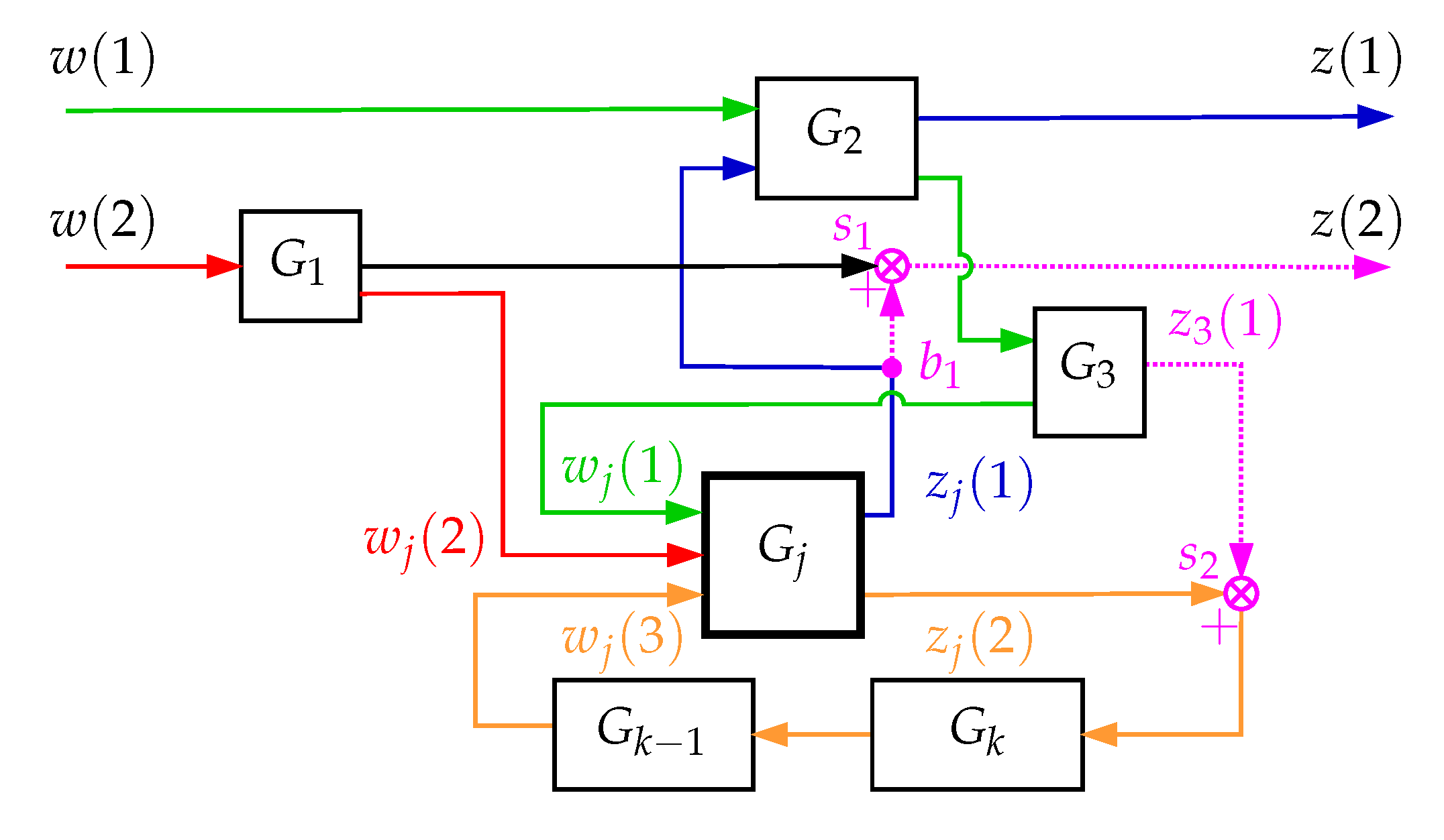
4.2. Defining the Unique Paths of Energy Transfer throughout the System

Let us now consider an example of an interconnected dynamical system, that is assumed to be dissipative, as represented with Figure 13. Dissipativity of the interconnected system manifests itself with the dissipativity on the subsystem level and/or through dissipative interconnections between them. For the example at hand, let us assume that there are two performance (external) inputs $w={(w\left(1\right),w\left(2\right))}^T$ and two performance (external) outputs $z={(z\left(1\right),z\left(2\right))}^T$. Similar vector expansion of internal inputs $w_j\in {\mathcal{L}}_2^{n_{w_j}}$ and internal outputs $z_j\in {\mathcal{L}}_2^{n_{z_j}}$ is assumed, where $n_{w_j}$ and $n_{z_j}$ represent the number of inputs and the number of outputs of the $G_j$-th subsystem, respectively. The main idea is to define all the unique paths through which the energy can transferred. To do so, we examine the inputs and outputs of each subsystem.

Let us for that purpose focus on the j-th subsystem $G_j$ that has three inputs $w_j={(w_j\left(1\right),w_j\left(2\right),w_j\left(3\right))}^T$ and two outputs $z_j={(z_j\left(1\right),z_j\left(2\right))}^T$. We can start by examining the energy transfer from external inputs w to the internal inputs $w_j$, of the subsystem $G_j$, and from internal outputs $z_j$ to the external outputs z. In order for the energy to transfer from the external input $w\left(1\right)$ to the first input of the subsystem $G_j$ it needs to take the path through the subsystems $G_2$ and $G_3$—this is the green coloured energy transfer path in Figure 13. Following the same procedure for the external input $w\left(2\right)$, the energy passes through the system $G_1$—before landing on the second input of the subsystem $G_j$—following the red coloured energy transfer path shown in Figure 13. On the other hand, if the energy path is followed from the first output of the subsystem $G_j$, it can be observed that it needs to pass through the subsystem $G_2$, before reaching the external output $z\left(1\right)$—following the blue coloured energy transfer path, as shown in Figure 13. It can also be observed that part of the energy is also transferred from the second internal output $z_j\left(2\right)$ of the subsystem $G_j$ to the the third internal input $w_r\left(3\right)$ of the subsystem $G_j$, and doing so passes through the subsystems $G_k$ and $G_{k-1}$—following the orange coloured path of energy transfer. It is also possible to take into account the branching points and summation points together with the accompanying energy transfer paths following the dashed pink coloured in Figure 13. By doing so, the following can be observed. Some of the energy is directly transferred from subsystem output $z_j\left(1\right)$ through the branching point $b_1$ and the summation point $s_1$ to the external output $z\left(2\right)$. Note, in this case, although the inputs to the summation point $s_1$ are $z_1\left(2\right)$ and $z_j\left(1\right)$, we are only interested in the energy transferred from the system at hand to the external output $z\left(2\right)$. Then again, some of the energy coming from the external input $w\left(1\right)$ passes through the subsystems $G_2$ and $G_3$ before arriving at the summation point $s_2$ and transferring energy through the subsystems $G_k$ and $G_{k-1}$ towards the internal input $w_j\left(3\right)$ of the subsystem $G_j$. In this case, since some of the energy from the external input $w\left(1\right)$ is being dissipated, we do include this channel at the summation point $s_2$.

4.3. Replacing the Surroundings of a Subsystem with Input-Output Transfer Functions

After all the distinct paths of energy transfer for the system at hand (i.e., $G_j$ in this case) are obtained, we can calculate the input-output transfer functions (IOTF) for each path of energy transfer. By doing so, it is possible to find the minimum number of systems that will be connected directly to the internal inputs and outputs of the subsystem at hand, replacing the complex structure of the overall environment of one particular subsystem at hand. To simplify the explanation and calculation for the example shown in Figure 13, let us examine the calculation in the complex frequency domain (s-domain) with signals $\widehat{w}$, ${\widehat{w}}_j$, $\widehat{z}$ and ${\widehat{z}}_j$ by taking the Laplace transform of external inputs signals w, internal inputs signals $w_j$, external outputs signals z and internal outputs signal $z_j$, respectively. For the case of LTI systems, calculation for the IOTF of the subsystem $G_j$ can be carried out as

$$\begin{array}{cc}\hfill G_{w\left(1\right)\to w_j\left(1\right)}& =\frac{{\widehat{w}}_j\left(1\right)}{\widehat{w}\left(1\right)}={\widehat{G}}_3{\widehat{G}}_2,\hfill \end{array}$$

(34)

$$\begin{array}{cc}\hfill G_{w\left(2\right)\to w_j\left(2\right)}& =\frac{{\widehat{w}}_j\left(2\right)}{\widehat{w}\left(2\right)}={\widehat{G}}_1,\hfill \end{array}$$

(35)

$$\begin{array}{cc}\hfill G_{z_j\left(1\right)\to z\left(1\right)}& =\frac{\widehat{z}\left(1\right)}{{\widehat{z}}_j\left(1\right)}={\widehat{G}}_2,\hfill \end{array}$$

(36)

$$\begin{array}{cc}\hfill G_{z_j\left(2\right)\to w_j\left(3\right)}& =\frac{{\widehat{w}}_j\left(3\right)}{{\widehat{z}}_j\left(2\right)}={\widehat{G}}_{k-1}{\widehat{G}}_k,\hfill \end{array}$$

(37)

$$\begin{array}{cc}\hfill G_{z_j\left(1\right)\to z\left(2\right)}& =\frac{\widehat{z}\left(1\right)}{{\widehat{z}}_j\left(1\right)}=I,\hfill \end{array}$$

(38)

$$\begin{array}{cc}\hfill G_{w\left(1\right)\to z_3\left(1\right)}& =\frac{{\widehat{z}}_3\left(1\right)}{\widehat{w}\left(1\right)}={\widehat{G}}_3{\widehat{G}}_2,\hfill \end{array}$$

(39)

where ${\widehat{G}}_1,{\widehat{G}}_2,{\widehat{G}}_3,{\widehat{G}}_{k-1}$ and ${\widehat{G}}_k$ are transfer functions of $G_1,G_2,G_3,G_{k-1}$ and $G_k$, respectively.

The summation points $s_1$ and $s_2$ are defined as algebraic relations

$$\begin{array}{c}\hfill z\left(1\right)=z_j\left(1\right)+z_3\left(1\right)\end{array}$$

(40)

$$\begin{array}{c}\hfill w_k\left(1\right)=z_j\left(2\right)+z_3\left(1\right).\end{array}$$

(41)

The interconnected system defined by Equations (34)–(41) can be represented as shown in Figure 14. For such an interconnected system, interconnection matrices can be made using the same procedure as outlined in Section 2.3. To make a distinction between the interconnection matrices for interconnecting the whole system, which from now on will be called global interconnection matrices, we will simply call these local IOTF connection matrices.

On the Calculation of the IOTFs and its Practical Applicability

Although the example shown in Figure 13 had taken into consideration many possible scenarios of interconnections, this part remains to be explored for other combinations of interconnection. For this particular example, all the external inputs and outputs are highly clustered together (i.e., in the top part of the interconnected system) in a sense that some external signal is injected close to where it is measured—the example of this might be active car suspension, i.e., measurements include the tyre kinematics while forces are acting on the active suspension, and car body representing the overall distant part of the system. Then there might be systems that have external inputs on one side and at a distant side the outputs are measured—for these kinds of systems the procedure is practically the same, and will, arguably, also result in relatively small number of IOTF systems. A practical example of such a system might include active cruise control, i.e., measurements are taken at the tyre, some energy is carried throughout the power-train system and some action is taken on the engine side. However, if the external inputs and outputs are highly dispersed—i.e., everywhere in the system there are external inputs and everywhere in the system measurements are taken—this procedure might not yield the expected results and might not give major practical advantage over regular non-preserving methods. It should be noted that this type of input-output arrangement is not a typical case in practical application of the control. Moreover, finding all the energy transfer paths for all the subsystems might be cumbersome. Although there might not be fully automatic way to create IOTF, there are ready made solutions that greatly improve the applicability as it will be mentioned in the numerical example. It should also be noted that, if some of the energy paths are omitted, the only consequence will be a (slightly) more conservative uncertainty model [17,38,43].

4.4. Refining the Additive Uncertainty Model

After all the IOTF are defined, we stress that it is possible to recalculate the new additive uncertainty models for the subsystem $G_j$, that is essentially scaled by its environment.

Assuming that the subsystem $G_j$ is somehow discretized and of reduced order (by using some MOR method) such that we have ${\tilde{G}}_j$. All the energy transfer paths are defined (as in Figure 13) and all the needed IOTF are calculated. If we also define all the local IOTF connection matrices we can than examine two composite systems with either $G_j$ or ${\tilde{G}}_j$ being central to our examination (as in Figure 14). Due to the dissipative nature of the subsystems and their mutual interconnections, from now on, we assume that a significant amount of the energy throughout the system was dissipated (damped)—in a sense, that if the response in the frequency domain is to be evaluated for any IOTF, the response will be rather smooth (without peaks of significant gain). For that matter, it makes sense not to use large order IOTF, initially obtained with unreduced subsystems. So, in the next stage of uncertainty design, reduced order IOTF will be used. For each IOTF defined with the Equations (34)–(41), we obtain a low-order cover filters by using logarithmic-Chebysev magnitude design. With this laid out, we obtained two composite subsystems $G_{j,e}$ and ${\tilde{G}}_{j,e}$ (here index e will stand for environment). Now, as already explained in Section 2.5, we can proceed with the calculation of the refined uncertainty model, with refined weighting filters $W_{j,2e}$ and $W_{j,1e}$ now being as shown in Figure 15.

5. Conclusions and Future Work

In this paper it is shown that it is possible to systematically model uncertainties arising both from spatial discretization and model order reduction. To obtain less conservative uncertainty models, a structure of the interconnected system needs to be preserved. A structure preserving algorithm that consists in partitioning the interconnected system is presented. For each subsystem of interest, partitions are made such that the input-output transfer functions (IOTFs) are calculated. IOTFs represent the energy transfer from external performance input to internal subsystem input, from internal subsystem output to external performance output, as well as from the internal subsystem output to the internal subsystem input (i.e., some feedback connection). These IOTFs are later approximated with low-order weights that essentially scale the amount of uncertainty, rendering obtained uncertainties less conservative, while keeping the overall order of the interconnected system low. This approach is shown not only to produce less conservative uncertainty models by making appropriate frequency weights for the originally obtained uncertainties, but also to introduce flexibility in both overall system modelling and uncertainty modelling. Finally, in order to validate if the models are suitable for controller synthesis, a robustness test for closed loop controller synthesis is carried out using the $\nu$-gap metric. The obtained $\nu$-gaps between newly obtained low-order robustly stable models and the nominal unreduced models, were relatively close to zero, which implies that a controller that stabilizes the original (unreduced) interconnected system will tend to stabilize the new low-order interconnected system as well [7,49].

An important advantage of this structure preserving algorithm lies in the flexibility of the design process—a single subsystem can be easily modified and reconnected using same connections to be re-evaluated in the robustness analysis. This fact comes especially useful if a spatially invariant interconnected dynamic system is analysed or a system that has repeating subsystems with the same geometric and material properties, as for such systems memory requirements can drastically reduce. It is also possible to use other or combine different MOR methods on a subsystem level. Another advantage of the proposed algorithm lies in the flexibility of uncertainty modelling—depending on the available allowed size for the distributed robust controller to be synthesized—a trade off can be made in terms of the uncertainty conservatism versus the controller size. Usage of integral quadratic constraints framework for robustness analysis and uncertainty modelling is in itself highly attractive—besides fitting conveniently with the proposed structure-preserving scheme—it can be used to capture other types of uncertainties that can be included in the overall robustness analysis with relative ease. Some typical uncertainties that might occur and can readily be analysed, in parallel with the current analysis, include norm-bounded nonlinearities (that are used to model neglected dynamics and modelling errors), sector bounded and slope-restricted nonlinearities (that can be used for, e.g., modelling nonlinearities in material properties), passive uncertainties/nonlinearities and parametric uncertainties (concretely in the presented example this might be used to model unknown parameters in mass, stiffness and damping) [25]. Another advantage of the IQC analysis is the guaranteed robust stability and robust performance achieved by finding feasible solution of convex optimization problem.

A possible limitation of the proposed procedure may occur for systems that have highly dispersed locations of performance (external) inputs and outputs. Also, a process of defining the IOTFs is rather manual. While the main drawback is the calculation of the IOTF in the system partitioning step—requiring subsequent calculation of the reduced order refined frequency weights—that are part of the, often computationally demanding, iterative process in the IQC analysis steps. Although a feasible solution to the IQC analysis guarantees robustness—the design procedure, although pragmatical, is still heuristic—and will result in a model that is at best sub-optimal.

Future work might include a construction of an a-priori frequency weighted filters for refined uncertainty models based on energy storage functions of partitioned input-output transfer functions through the dissipation theory and integral quadratic constraints. Another interesting research direction may be to consider application of the proposed procedure on the systems that exhibit additional special properties—such as passivity and positive realness—that neatly intertwine with the theory of dissipativity, as this could result in further reduction in uncertainty conservatism and perhaps other fruitful insights into this topic [19]. A practical future work direction would be to develop a ready-to-use with MATLAB toolbox, based on the proposed procedure and previously pointed out future work directions. The proposed design procedure requires a lot of manual inputs and interpretations from a human and as such it could possibly be carried out using type-3 fuzzy logic systems framework [50].

References

1. Bathe, K.J. (Ed.) Finite Element Procedures, 2nd ed.; Prentice Hall, Pearson Education, Inc.: Watertown, MA, USA, 2014. [Google Scholar]
2. Bathe, K.J. Finite Element Procedures in Engineering Analysis; Prentice-Hall Civil Engineering and Engineering Mechanics Series; Prentice-Hall: Englewood Cliffs, NJ, USA, 1982. [Google Scholar]
3. Hughes, T.J.R. The Finite Element Method: Linear Static and Dynamic Finite Element Analysis; Dover Publications: New York, NY, USA, 2000. [Google Scholar]
4. Srivastava, V.; Dwivedi, S.; Mukhopadhyay, A. Parametric Investigation of Vibration of Stiffened Structural Steel Plates Using Finite Element Analysis and Grey Relational Analysis. Rep. Mech. Eng. 2022, 3, 108–115. [Google Scholar] [CrossRef]
5. Jokic, M.; Stegic, M.; Butkovic, M. Reduced-Order Multiple Tuned Mass Damper Optimization: A Bounded Real Lemma for Descriptor Systems Approach. J. Sound Vib. 2011, 330, 5259–5268. [Google Scholar] [CrossRef]
6. Jones, B.L.; Kerrigan, E.C. When Is the Discretization of a Spatially Distributed System Good Enough for Control? Automatica 2010, 46, 1462–1468. [Google Scholar] [CrossRef] [Green Version]
7. Vinnicombe, G. Uncertainty and Feedback: H [Infinity] Loop-Shaping and the [Nu]-Gap Metric; Imperial College Press: London, UK, 2001. [Google Scholar]
8. Antoulas, A.C. Approximation of Large-Scale Dynamical Systems; Advances in Design and Control, Society for Industrial and Applied Mathematics: Philadelphia, PA, USA, 2005. [Google Scholar]
9. Reis, T.; Stykel, T. Passivity-Preserving Model Reduction of Differential-Algebraic Equations in Circuit Simulation. PAMM 2007, 7, 1021601–1021602. [Google Scholar] [CrossRef]
10. Schwerdtner, P.; Voigt, M.; Voigt, M. Structure Preserving Model Order Reduction by Parameter Optimization. arXiv 2020, arXiv:2011.07567. [Google Scholar]
11. Beddig, R.S.; Benner, P.; Dorschky, I.; Reis, T.; Schwerdtner, P.; Voigt, M.; Voigt, M.; Werner, S.W.R. Structure-Preserving Model Reduction for Dissipative Mechanical Systems. arXiv 2020, arXiv:2010.06331. [Google Scholar]
12. Cheng, X.; Scherpen, J.M. Model Reduction Methods for Complex Network Systems. arXiv 2020, arXiv:2012.02268. [Google Scholar] [CrossRef]
13. Wu, F.; Wang, Z.; Song, D.; Lian, H. Lightweight Design of Control Arm Combining Load Path Analysis and Biological Characteristics. Rep. Mech. Eng. 2022, 3, 71–82. [Google Scholar] [CrossRef]
14. Reis, T.; Stykel, T. Stability Analysis and Model Order Reduction of Coupled Systems. Math. Comput. Model. Dyn. Syst. 2007, 13, 413–436. [Google Scholar] [CrossRef]
15. Dogančić, B.; Jokić, M. Discretization and Model Reduction Error Estimation of Interconnected Dynamical Systems. Ifac Pap. 2022; in press. [Google Scholar]
16. Stefanović-Marinović, J.; Vrcan, Ž.; Troha, S.; Milovančević, M. Optimization of Two-Speed Planetary Gearbox with Brakes on Single Shafts. Rep. Mech. Eng. 2022, 3, 94–107. [Google Scholar] [CrossRef]
17. Scherer, C.W.; Weiland, S. Linear Matrix Inequalities in Control. 2015. Available online: https://www.imng.uni-stuttgart.de/mst/files/LectureNotes.pdf (accessed on 12 January 2022).
18. Scherer, C.W.; Veenman, J. Stability Analysis by Dynamic Dissipation Inequalities: On Merging Frequency-Domain Techniques with Time-Domain Conditions. Syst. Control Lett. 2018, 121, 7–15. [Google Scholar] [CrossRef] [Green Version]
19. Scherer, C. Dissipativity and Integral Quadratic Constraints, Tailored Computational Robustness Tests for Complex Interconnections. arXiv 2022, arXiv:2105.07401. [Google Scholar] [CrossRef]
20. Willems, J.C. Dissipative Dynamical Systems Part I: General Theory. Arch. Ration. Mech. Anal. 1972, 45, 321–351. [Google Scholar] [CrossRef]
21. Willems, J.C. Dissipative Dynamical Systems Part II: Linear Systems with Quadratic Supply Rates. Arch. Ration. Mech. Anal. 1972, 45, 352–393. [Google Scholar] [CrossRef]
22. Balas, G.; Doyle, J.; Glover, K.; Packard, A.; Smith, R. μ-Analysis and Synthesis Toolbox; The MathWorks Inc.: Natick, MA, USA; MYSYNC Inc.: Natick, MA, USA, 1995. [Google Scholar]
23. Balas, G.J.; Chiang, R.Y.; Packard, A.; Safonov, M.G. Robust Control Toolbox™ User’s Guide; The MathWorks Inc.: Natick, MA, USA, 2021. [Google Scholar]
24. Megretski, A.; Rantzer, A. System Analysis via Integral Quadratic Constraints. IEEE Trans. Autom. Control. 1997, 42, 819–830. [Google Scholar] [CrossRef] [Green Version]
25. Veenman, J.; Scherer, C.W.; Köroğlu, H. Robust Stability and Performance Analysis Based on Integral Quadratic Constraints. Eur. J. Control. 2016, 31, 1–32. [Google Scholar] [CrossRef]
26. Veenman, J.; Scherer, C.W.; Ardura, C.; Bennani, S.; Preda, V.; Girouart, B. IQClab: A New IQC Based Toolbox for Robustness Analysis and Control Design. IFAC-Pap. 2021, 54, 69–74. [Google Scholar] [CrossRef]
27. Gahinet, P.; Nemirovskii, A. General-Purpose LMI Solvers with Benchmarks. In Proceedings of the 32nd IEEE Conference on Decision and Control, San Antonio, TX, USA, 15–17 December 1993; Volume 4, pp. 3162–3165. [Google Scholar] [CrossRef]
28. Gahinet, P.; Nemirovskii, A.; Laub, A.; Chilali, M. The LMI Control Toolbox. In Proceedings of the 33rd IEEE Conference on Decision and Control, Lake Buena Vista, FL, USA, 14–16 December 1994; Volume 3, pp. 2038–2041. [Google Scholar] [CrossRef]
29. Löfberg, J. YALMIP: A Toolbox for Modeling and Optimization in MATLAB. In Proceedings of the CACSD Conference, Boston, MA, USA, 30 June–2 July 2004. [Google Scholar]
30. Grant, M.; Boyd, S. Graph Implementations for Nonsmooth Convex Programs. In Recent Advances in Learning and Control; Blondel, V., Boyd, S., Kimura, H., Eds.; Lecture Notes in Control and Information Sciences, Springer-Verlag Limited: London, UK, 2008; pp. 95–110. [Google Scholar]
31. Grant, M.; Boyd, S. CVX: Matlab Software for Disciplined Convex Programming, Version 2.1, 2014. Available online: http://cvxr.com/cvx (accessed on 13 March 2022).
32. Sturm, J.F. Using SeDuMi 1.02, A MATLAB Toolbox for Optimization over Symmetric Cones. Optim. Methods Softw. 1999, 11, 625–653. [Google Scholar] [CrossRef]
33. Toh, K.C.; Todd, M.J.; Tütüncü, R.H. SDPT3—A Matlab Software Package for Semidefinite Programming, Version 1.3. Optim. Methods Softw. 1999, 11, 545–581. [Google Scholar] [CrossRef]
34. ApS, M. The MOSEK Optimization Toolbox for MATLAB Manual. Version 9.2; MOSEK ApS: Copenhagen, Denmark, 2020. [Google Scholar]
35. Reis, T.; Stykel, T. Balanced Truncation Model Reduction of Second-Order Systems. Math. Comput. Model. Dyn. Syst. 2008, 14, 391–406. [Google Scholar] [CrossRef]
36. Reis, T.; Stykel, T. PABTEC: Passivity-preserving Balanced Truncation for Electrical Circuits. IEEE Trans. Comput. Aided Des. Integr. Circuits Syst. 2010, 29, 1354–1367. [Google Scholar] [CrossRef]
37. Boyd, S.; Ghaoui, L.E.; Feron, E.; Balakrishnan, V. Linear Matrix Inequalities in System and Control Theory; Studies in Applied Mathematics; SIAM: Philadelphia, PA, USA, 1994; Volume 15. [Google Scholar]
38. Boyd, S.; Vandenberghe, L. Convex Optimization; Cambridge University Press: Cambridge, UK, 2004. [Google Scholar]
39. Salehi, Z.; Karimaghaee, P.; Khooban, M.H. A New Passivity Preserving Model Order Reduction Method: Conic Positive Real Balanced Truncation Method. IEEE Trans. Syst. Man Cybern. 2021, 52, 2945–2953. [Google Scholar] [CrossRef]
40. Salehi, Z.; Karimaghaee, P.; Khooban, M.H. Model Order Reduction of Positive Real Systems Based on Mixed Gramian Balanced Truncation with Error Bounds. Circuits Syst. Signal Process. 2021, 40, 5309–5327. [Google Scholar] [CrossRef]
41. Wang, X.; Fan, S.; Dai, M.Z.; Zhang, C. On Model Order Reduction of Interconnect Circuit Network: A Fast and Accurate Method. Mathematics 2021, 9, 1248. [Google Scholar] [CrossRef]
42. Reis, T.; Stykel, T. Positive Real and Bounded Real Balancing for Model Reduction of Descriptor Systems. Int. J. Control. 2010, 83, 74–88. [Google Scholar] [CrossRef]
43. Skogestad, S.; Postlethwaite, I. Multivariable Feedback Control: Analysis and Design, 2nd ed.; Wiley: Chichester, UK, 2010. [Google Scholar]
44. D’Andrea, R. Convex and Finite-Dimensional Conditions for Controller Synthesis with Dynamic Integral Constraints. IEEE Trans. Autom. Control. 2001, 46, 222–234. [Google Scholar] [CrossRef]
45. Dogancic, B.; Jokic, M.; Alujevic, N.; Wolf, H. Unstructured Uncertainty Modeling for Coupled Vibration Systems. In Proceedings of (ISMA2018)/(USD2018); Desmet, W., Pluymers, B., Moens, D., Rottiers, W., Eds.; Katholieke Universiteit Leuven: Leuven, Belgium, 2018; pp. 5125–5132. [Google Scholar]
46. Dogančić, B. Bruno-Dogancic/Spumbox. GitHub: San Francisco, CA, USA, 2022. Available online: https://github.com/bruno-dogancic/spumbox (accessed on 12 January 2022).
47. Dogančić, B. Bruno-Dogancic/Spumbox: Spumbox_v0.1; Zenodo (CERN): Geneva, Switzerland, 2022. [Google Scholar] [CrossRef]
48. Oppenheim, A.V.; Schafer, R.W. Digital Signal Processing; Prentice-Hall: Englewood Cliffs, NJ, USA, 1975. [Google Scholar]
49. Vinnicombe, G. On IQCs and the /Spl Nu/-Gap Metric. In Proceedings of the 37th IEEE Conference on Decision and Control (Cat. No.98CH36171), Tampa, FL, USA, 18–18 December 1998; Volume 2, pp. 1199–1200. [Google Scholar] [CrossRef]
50. Mosavi, A.; Qasem, N.; Shokri, M.; Band, S.S.; Mohammadzadeh, A. Fractional-Order Fuzzy Control Approach for Photovoltaic/Battery Systems under Unknown Dynamics, Variable Irradiation and Temperature. Electronics 2020, 9, 1455. [Google Scholar] [CrossRef]
Figure 1. Modelling the absolute error between the original model and the reduced order discretized model as an uncertain dynamical system with additive uncertainty: (a) Adding the absolute error G j G j ˜ to the reduced order discretized model G j ˜ . (b) Representing the absolute error as an additive uncertainty W j , 2 Δ j W j , 1 .
Mathematics 10 02125 g001
Figure 2. Standard feedback interconnection for robustness analysis.
Mathematics 10 02125 g002
Figure 3. A preprocessing step for obtaining and storing of arrays of LTI models: reference models ( G j ) and discretized reduced order models ( G ˜ j , n j , m j ). For each discretized system, n j = 1 , , n j D discretized LTI models are made. For discretized models, a reference model is created by choosing the best available discretization (i.e., n j = n j D ) that is reduced using high fidelity balanced truncation method—a step analogous to obtaining a minimal realization. For each reduced order model, Hankel singular values are calculated and only first m j = 1 , , m j H S V models are stored. It should be noted that the discretization step (i) can be carried out using readily available FEA/FEM or meshing software.
Mathematics 10 02125 g003
Figure 4. Structure of the system is used to obtain the insight into how energy is being dissipated (damped) inside the system. Interconnection matrices are used to create interconnected reference system and interconnected uncertain systems (a) complex interconnections (or surroundings, environment) around each subsystem are essentially acting as scaling filters at input and output of each subsystem (input output transfer functions-IOTFs). These scaling filters (IOTFs) are reduced and used to calculate a low order scaled versions of both the reference model and discretized reduced order model. (b) Once the interconnection matrices R,K and H have been created, and a reference interconnected system is obtained (i.e., G)-uncertain interconnected system(s) can also be obtained using the same interconnection matrices and replacing the appropriate reference subsystems with the relevant uncertain subsystems (i.e., replace G j with G j , s u , G j , e u or G j u ).
Mathematics 10 02125 g004
Figure 5. Uncertainty modelling and uncertainty refinement through the creation of weights W j , 1 and W j , 1 e , respectively. Calculating the absolute error and obtaining weights for each subsystem, without taking into account the (dissipative) surroundings of the subsystem yields conservative results (i.e., W j , 1 , a process denoted as (vii)). Calculating the absolute errors for each subsystem that is scaled by its surroundings and turning it into refined weights W j , 1 e , results in lower magnitude in frequency response in wide frequency range—hence less conservative uncertainty model was achieved. The scaled weights can often be further simplified by simply replacing it by its peak response—this offers a flexible and useful trade-of—reduce the order of the weights (i.e., no additional states are introduced with weights of static (constant) gain response) at introduction of some conservatism, or vice versa. The steps needed to obtain the weights of static gain W j , 1 s , are denoted as (vi).
Mathematics 10 02125 g005
Figure 6. Carry out IQC analysis and optional postprocessing (if the IQC analysis was successful) for a given nominal parts of uncertain system(s) Γ s ( Γ e , Γ ) and check if all the robustness criteria are satisfied. (a) Decision making process 1 (DMP1)-if a feasible solution cannot be found and/or performance criterion cannot be met with a Γ s , try Γ e or Γ . (b) IQC analysis process and decision making process 2 (DMP2)-if there is no feasible solution found to the IQC analysis appropriate changes have to be made; either to the IQC analysis parameters or the uncertain system (see Figure 7 for further details), if there was feasible solution found, but the specified performance criterion has not been met, then the discretizations and/or orders of the reduced order models are too low and have to be adjusted. (c) Continue to optional post-processing—i.e., carry out robustness analysis using μ -tools instead of IQCs, run ν -gap analysis or perform frequency and/or time domain simulations to confirm the desired behaviour of the obtained uncertain interconnected system.
Mathematics 10 02125 g006
Figure 7. Decision making process 3 (DMP3)—The suggested order of adjustments that have to be made to the IQC analysis parameters and to the uncertain interconnected system to satisfy a given robustness criteria. First decision (D1) reflects the changes are being made to the IQC parameters (i.e., v and ρ ). Other decisions reflect the changes are being made to the uncertain interconnected system. Changes are being made to the orders of uncertainty weights first (D2), then to the orders of reduced order IOTFs (D3) and after that to the level of discretizations of subsystems (i.e., n j ) and/or to the orders of the model order reduced subsystems (i.e., m j )—collectively the fourth decision (D4).
Mathematics 10 02125 g007
Figure 8. A series of simply supported Euler beams mutually interconnected by springs and dampers: (a) Mechanical schematic of an interconnected system. (b) Block diagram representation of the system, where the systems with odd indices, i.e., G 1 , G 3 , G j , , G k are dynamical systems representing LTI models of discretized beams, while the systems with even indices, i.e., G 2 , G 4 , G j 1 , , G k 1 are the systems of static gain representing springs and dampers between each beam.
Mathematics 10 02125 g008
Figure 9. Frequency response of the original (unreduced) interconnected system compared to RO (Reduced Order with initially calculated weights W j , 1 ), RW (reduced order with Refined Weights W j , 1 e ) and SW (reduced order with Static Weights W j , 1 s ). (a) Case #1, beams mutually interconnected only by dampers, representing a highly dissipative case. (b) Case #2, beams mutually interconnected only by springs, representing the least dissipative (stiffest) case. (c) Case #3, beams mutually interconnected by both dampers and springs, representing the most complex interconnections case (with most uncertainty channels).
Mathematics 10 02125 g009
Figure 10. Frequency response of the with initially calculated weights W j , 1 (solid black line), refined weights W j , 1 e (dash-dot red line) and static weights W j , 1 s (dashed green line). (a) Case #1, system 3. (b) Case #1, system 11. (c) Case #1, system 19. (d) Case #2, system 3. (e) Case #2, system 7. (f) Case #2, system 13. (g) Case #3, system 3. (h) Case #3, system 5. (i) Case #3, system 9.
Mathematics 10 02125 g010
Figure 11. Case #1 with different n j and m j . Using higher discretization and higher order for the first subsystem, results in a better correlation in the frequency response when compared to the original system. Few random uncertainty samples are shown to give an idea of the frequency response of the uncertain interconnected system.
Mathematics 10 02125 g011
Figure 12. Examples of the different low-order weights (filters)—modelled using logarithmic-Chebyshev filter design—that cover the frequency response of a high order dynamical system in the desired frequency range. All lower order filters are stable and modelled in such a way to have gain larger than the original high order dynamical system. This makes such a filter useful when modelling unstructured uncertainties (e.g., additive uncertainty).
Mathematics 10 02125 g012
Figure 13. Example of the interconnected dissipative dynamical system. Defining the paths of energy transfer to and from the subsystem G j .
Mathematics 10 02125 g013
Figure 14. Obtaining the composite subsystems G j , e and G ˜ j , e , scaled by its environment, by connecting the reduced order input-output transfer functions (IOTF) to the inputs and outputs of the examined subsystem G j or reduced order subsystem G ˜ j , respectively.
Mathematics 10 02125 g014
Figure 15. Uncertainty refinement—calculating the scaled frequency weighting filter W j , 1 e : (a) Representation of the absolute error between the nominal scaled subsystem G j , e and the reduced order scaled subsystem G ˜ j , e . (b) Representing the absolute error as an additive uncertainty with the new refined frequency weighting filters W j , 2 e and W j , 1 e .
Mathematics 10 02125 g015