
The Complexity of Cryptocurrencies Algorithmic Trading


1
Department of Management, Western Galilee Academic College, Acre 2412101, Israel
2
School of Business Administration, University of Haifa, Haifa 3498838, Israel
*
Author to whom correspondence should be addressed.
Mathematics 2022, 10(12), 2037; https://doi.org/10.3390/math10122037
Submission received: 8 May 2022
/
Revised: 7 June 2022
/
Accepted: 10 June 2022
/
Published: 12 June 2022
(This article belongs to the Special Issue Mathematical Aspects of Trading and Valuating Financial Assets)
Abstract
:In this research, we provided an answer to a very important trading question, what is the optimal number of technical tools in order to achieve the best trading results for both swing trade that uses daily bars and intraday trade that uses minutes bars? We designed Machine Learning (ML) systems that can trade four major cryptocurrencies: Bitcoin, Ethereum, BNB, and Solana. We found that more indicators do not necessarily mean better trading performance. Swing traders that use daily bars should trade Bitcoin and Solana using Ichimoku Cloud (IC) plus Moving Average Convergence Divergence (MACD), Ethereum with IC plus Chaikin Money Flow (CMF), and BNB with IC alone. With regard to intraday trading, we documented that different cryptocurrencies should be trading using different time frames. These results emphasize that the optimal number of indicators that are used to trade daily bars is one or, at maximum, two. The Multi-Layer (MUL) system that consists of all three examined technical indicators failed to improve the trading results for both days (swing) and intraday trades. The main implication of this study for traders is that more indicators does not necessarily improve trades performances.
1. Introduction
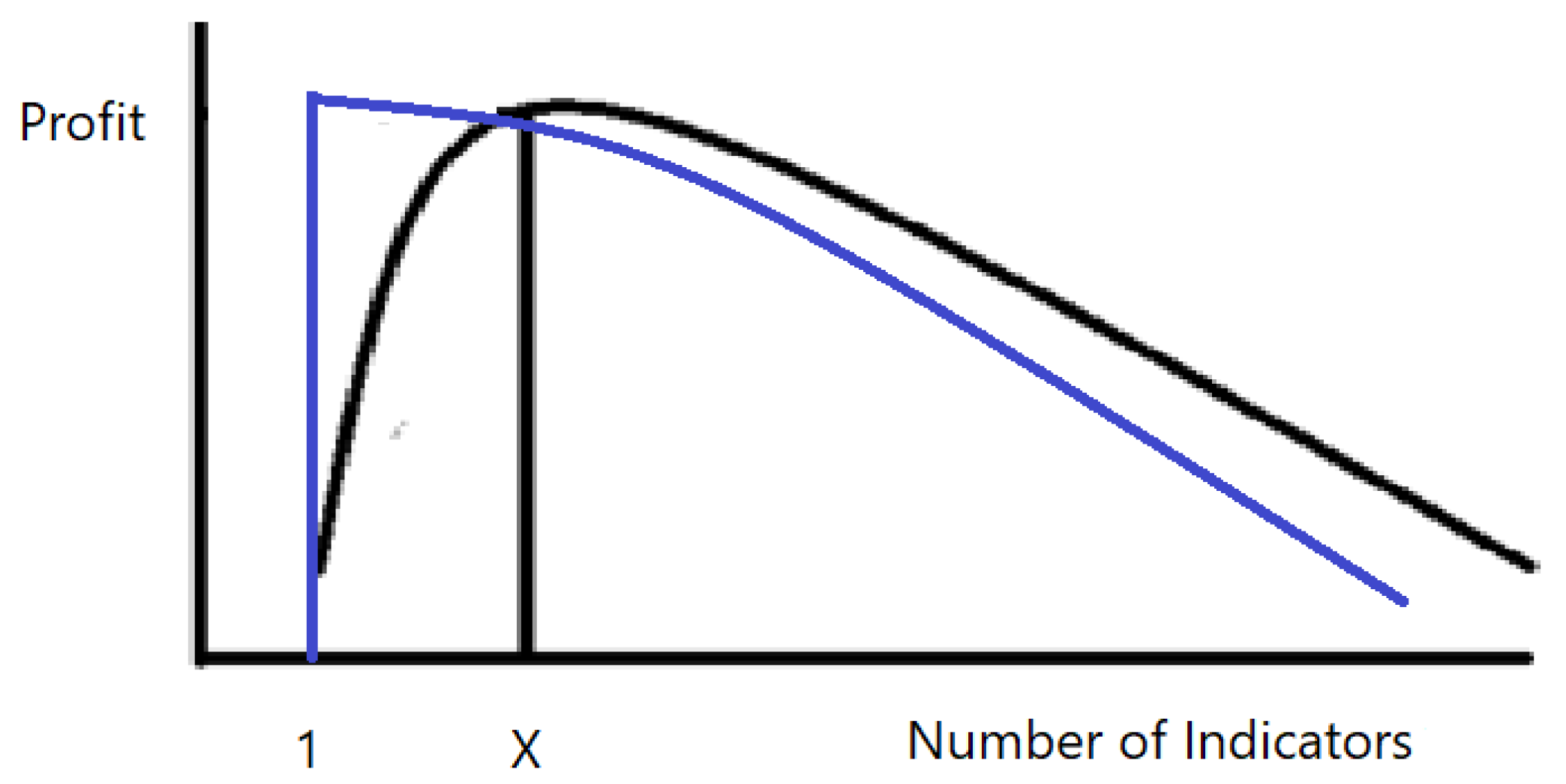
Forecasting the financial market direction has noalways been challenging and complex because of the multiple factors that simultaneously influence financial assets’ price. In recent years, Machine Learning (ML) based on deep Neural Networks (NN) has contributed dramatically to the forecasting ability. Those systems are not only designed for price forecasting of financial assets, but also for algorithmic trading. The input of such a system is typically sequential past prices and volumes that are processed by mathematical calculation and produce a numeric valuation that enables the system to calculate the probabilities for trend continuity or reversal. The designer of such a system lay layers of conditions that are based on technical analysis, which determines when to enter or exit a trade (long or short). As the conditions are mounted, the system will wait until all required conditions are met to engage in trading. This in many cases results in a late entry/exit of a trade to a point where a price reversal is more likely to occur than the continuation of the current trend. Researchers have tried in the past to implement different trading strategies for different financial assets. Most of them (see for example Ref. [1]) have test trading profitability according to a single trading indicator or methodology. The present study compares trading results of a single indicators system to a Multiple Layers (MUL) system that is comprised of several indicators combined. Our challenge is to find how many indicators should be incorporated into the ML system to ensure fast enough entry and exit of trade without neglecting important signals that could result in the wrong prediction. This dilemma has not been fully explored in the literature, and the current paper wants to bridge that existing gap. As shown in Figure 1, adding indicators to the designed trading system may increase profitability until the marginal technical tool does not contribute to the profit. In that case, the optimum number of indicators that guide the ML system should be X. On the other hand, the optimal level of indicators may be a single indicator, meaning that adding more indicators will cause profit to drop, and therefore should be avoided.
In the following research, we test stand-alone three indicator systems and then formed a dual indicator system and eventually Multi-Layer (MUL), which combines all three tools into one system. We seek the optimal combinations of technical tools incorporated into our NN system that will lead to a maximum profit trading cryptocurrencies using daily data (swing trade) and intraday data. Our data contain 5, 15, 30, 45, 60, and 120 min trading bars (a trading bar includes the opening and closing price of the specified time frame along with the highest and lowest prices) along with daily bars of four major cryptocurrencies: Bitcoin, Ethereum BNB (Binance Coins), and Solana from the beginning of 2021 till the end of April 2022.
We find that more indicators do not necessarily mean better trading performance. The best stand-alone indicator to trade daily bars of all examined cryptocurrencies was found to be Ichimoku Cloud (IC). Adding Moving Average Convergence Divergence MACD to IC improved performance, trading Bitcoin and Solana while adding Chaikin Money Flow (CMF) improved the trading results of Ethereum. BNB best performing system relied only on IC. With regard to intraday trading, the best performances were achieved by a single indicator system.
2. Literature Review
The complexity of financial asset price forecasting often drives researchers to use NN-based systems because of their ability to handle big data that originated from different sources of information (see for example: [2,3,4]). The evolution of this field has led researchers to construct more complex networks that are based on transformed data rather than the standard raw data. Ref. [5] used a radical basic function NN that transforms input signals before they are fed to the networks. They concluded their system is superior to more traditional NN in both trading performance and statistical accuracy. Long Short-Term Memory (LSTM) systems include three stages—input, forget and output—that control the flow of information over time, and therefore suit time series analysis. The challenge that this methodology introduces is to set the time frames for the memory and forget periods. The wrong setting may result in a set of data that confuses the algorithmic system and can lead to bad trading performances. Ref. [6] studies the usage of LSTM networks to predict future trends of stock prices based on past prices. Their results showed an average of 55.9% accuracy in predicting stock uptrends in the near future. Ref. [7] used Long Short-Term Memory (LSTM) system to predict the S & P500 index and concluded that this type of forecasting method is superior to other machine learning methods. Ref. [8] used the LSTM model to predict the direction of the Chinese stocks and showed a 13% forecasting improvement compared to other methods. Ref. [9] used LSTM for intraday stock prediction using technical analysis indicators as network inputs and found that their model performs better than the benchmark or equally weighted ensembles. Ref. [10] used transformed NN using indicators like relative strength index to predict future prices and concluded that incorporating domain knowledge in NN improves price prediction.
NN systems are also being used to predict the volatility of the financial asset. Ref. [11] combined the GARCH model with NN and compared their model to the classical GARCH model and found that the hybrid model is superior to the classical model in prediction volatility. Ref. [12] proved that ARMA-GARCH with artificial neural networks can effectively predict market shocks.
Cryptocurrency prices suffer from a highly volatile trading environment that can benefit from algorithmic trading systems (see for example Ref. [13,14]). Ref. [15] examined the cryptocurrency exchanges’ effects on prices and concluded that the shared information is dynamic and has a significant impact on investors. Ref. [16] modeled interaction in discontinuous movements of cryptocurrencies and showed that small price jumps observed in cryptocurrencies negatively affect the jump component of other cryptocurrencies’ realized volatility, while large jumps have the opposite effect. They also documented a negative effect of S & P500 jumps on cryptocurrency price jumps. In the current study, we also documented discontinuous movements of some of the examined cryptocurrencies that made future price forecasting more challenging. However, this phenomenon is mitigated as we moved to smaller periods of time frames.
3. Materials and Methods
Our intention in this research is to examine the optimal number of indicators that will produce the best trading performances for both minutes and daily bars. Our algorithmic trading system uses a single standalone indicator and compares its performances to integrated systems that use two and three indicators together. Our null hypothesis is as follows:
Hypothesis 0 (H0).
More indicators will improve trading performances.
Our data contain minutes of various trading bars of sizes along with daily bars of four major cryptocurrencies: Bitcoin, Ethereum BNB (Binance Coins), and Solana from January 2021 till April 2022. These cryptocurrencies were selected because of their market value and volumes of trade (The data was retrieved from investing.com).
3.1. Recurrent Neural Networks
The nature of the financial markets data is derived from the emergence of Recurrent Neural Networks (RNN). Unlike standard NN procedures that only learn from training data, Recurrent Neural Network (RNN) can also use past states to process its inputs and improve the system predictions abilities [17]. Since financial asset price prediction is complex and depends on various inputs, a complex-valued weights RNN is needed [18,19]. The RNN goal is to get a predicted value that is as close as possible to the actual value. At time , is obtained through a channel estimation that uses a series of past values: , that are fed into the RNN (, are example values, however, the model can integrate as many values as needed). The input of the system is denoted in Equation (1), while the output and the prediction channel are presented in Equations (2) and (3).
We utilized the RNN procedure by using inputs calculation derived from three different technical tools. These calculations are then used together as filters of our system that determines the actual entry and exit of a trade.
3.2. The Trading Strategy
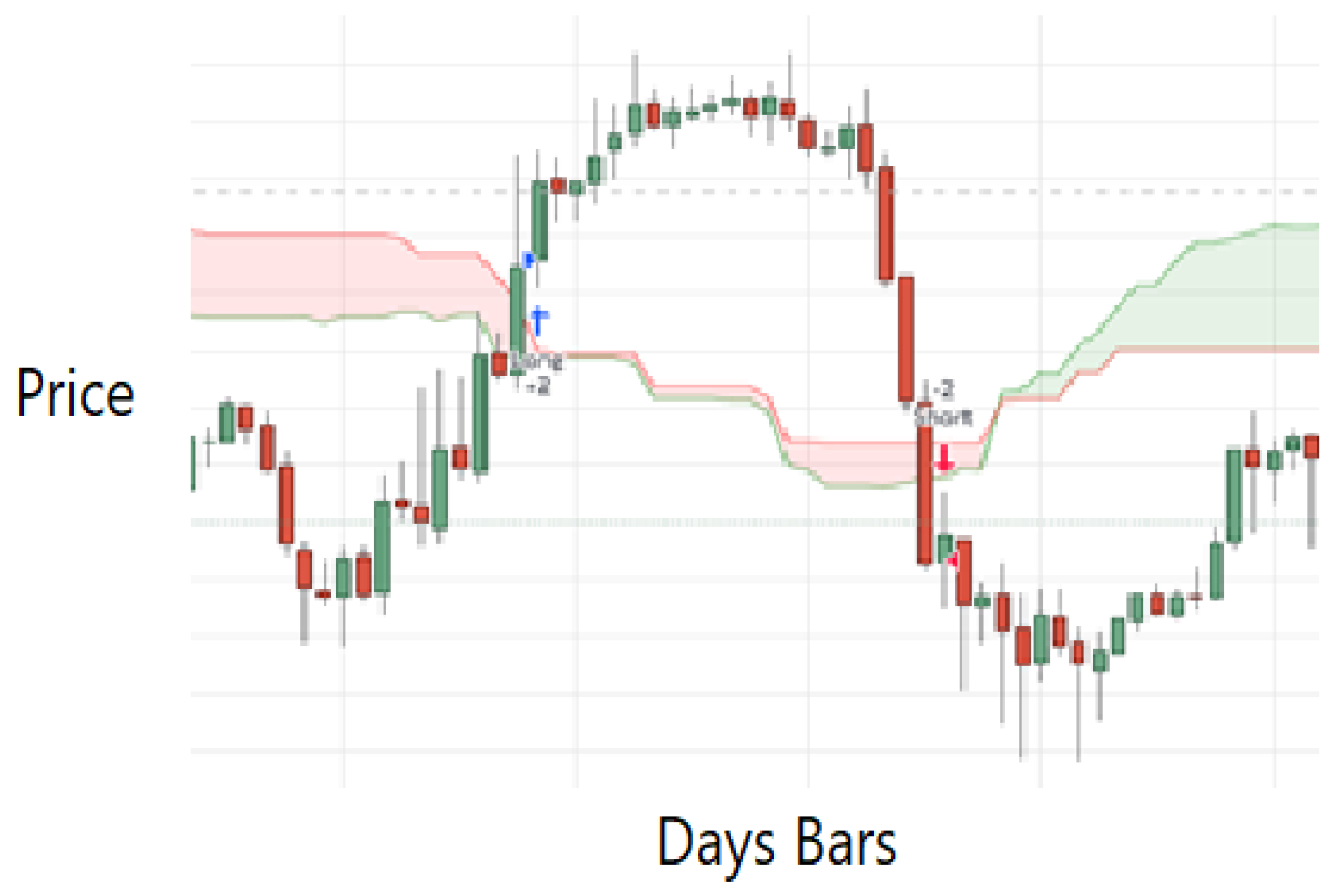
Our trading strategy is based primarily on Ichimoku Cloud (IC) indicator developed by Goich Hosoda. The indicator points to momentum and trend direction along with using multiple averages that create a cloud shape figure that helps traders to detect the market direction and support and resistance eras. As shown in Figure 2, when the price of the financial asset is above the cloud, the trend is up, and the system enters a long position and when the price is below the cloud the trend is down and the system enters a short position. In addition to IC we incorporate into our system two other trading indicators CMF and MACD.
Chaikin Money Flow (CMF) developed by Marc Chaikin is a volume-weighted average of accumulation and distribution over a specified period. The contribution of CMF to our trading system is its ability to identify market direction by integrating trade volumes with price movements. Above zero CMF is serves as an uptrend signal while below zero scores is a downtrend signal. MACD is a trend momentum indicator that measures the difference between two Exponential Moving Averages (EMA) (the exponential moving average is a moving average that places a greater weight on the most recent data than older data) of a financial asset’s price. When the MACD crosses above its signal line (the signal line is a nine-day EMA of the MACD), an uptrend is predicted and when the MACD crosses below its signal line a downtrend is predicted. The long entry conditions are described in Equations (4)–(7) and the short entry conditions are described in Equations (8–(11). Conditions 4 and 5 for long trades and 8 and 9 for short trades are derived from IC calculations, while Conditions 6 and 10 (long and short) are derived from the CMF indicator calculations, and 7 and 11 (long and short) are derived from the MACD formula.
Long Conditions:
Short Conditions:
where: p = closing price, PH = period high, PL = period low, V = period trading volume, = twelve periods exponential moving average, = twenty-six periods of the exponential moving average.
We start by constructing and testing a trading system using each indicator as a stand-alone algorithmized trading tool for both intraday and multiple days trading of the examined cryptocurrencies. We then combined IC with MACD conditions to create a system that is based on the accumulation of two indicators and repeated that process for IC and CMF as well. Finally, we constructed Multiple Layers (MUL) system that is based on the accumulation of the three indicators CI + MACD + CMF. Our aim is to find out if different cryptocurrencies demand different trading tools and what is the optimal number of indicators that will result in maximum Net Profit (NP) for each crypto and time frame. Along with the NP, our algorithm is designed to calculate and report real-time Profit Factor (PF), which is the gross profit divided by gross losses, and the percent of profitable trades of all trades (PP). The system operates on different time frames bars including 5, 15, 30,45, 60, and 120 min and on daily bars.
4. Results
We start by presenting in Table 1 the trading results of our RNN system using IC indicator as a stand-alone indicator generating calculations that are fed to the system to generate real-time buy and sell signals.
Table 1 demonstrates that IC based system best be used to trade daily bars resulting in an average remarkable PF of 4.43 and PP of 51%. The highest PF was achieved for Bitcoin Daily Bars trades followed by Solana and BNB. With regard to intraday trading, 60 min bars are the most prominent for Bitcoin, 45 min for Ethereum and Solana, and 120 min for BNB. Table 2 summarizes the results of the CMF as a stand-alone indicator that its calculations are fed to our system and determine trades entry and exit.
Table 2 shows that all cryptocurrencies are traded profitably using daily bars with an average of 1.18 PF and 51.6% PP. In terms of intraday trades, 45 min are the best time frames to analyze and trade Bitcoin and Ethereum, 30 min for BNB, and 5 min for Solana. Table 3 shows the results of our RNN system based on MACD as a stand-alone indicator.
Table 3 show that daily bars generate profitable trades trading Bitcoin, Ethereum, and Solana, but not BNB using the MACD indicator. Regarding intraday trades, the system generated the most profitable trades using 60 min bars for Bitcoin, Ethereum, and Solana, and 45 min bars for BNB. Concluding the single indicator systems, the best indicator to trade daily bars is by far IC, resulting in an average PF of 4.43 compared to 1.18 and 1.2 for the CMF and MACD, respectively. In terms of intraday trades, the best configuration for Bitcoin and Ethereum is CMF 45 min bars resulting in 70,675$ NP and 56.8% PP for Bitcoin and 2820$ NP and 54.7% PP for Ethereum. BNB is best-traded intraday using 120 min bar and IC resulting in 578$ NP and 1.53 PF. We now apply dual layers sets of conditions to our RNN systems and start by analyzing the trading results of IC and MACD systems.
Table 4 demonstrates that the combination of IC and MACD has led to a profit for all four cryptocurrencies trading daily bars with a high average PF of 3.75, which is lower than the average PF using IC, which was found to be the most effective indicator for trading cryptocurrencies daily bars. While incorporating MACD with IC has slightly improved the results of the daily-based system for Bitcoin than the stand-alone IC system, it dramatically reduces the results for BNB trades since, as Table 3 pointed out, MACD is not a useful technical indicator to trade BNB daily bars. In terms of intraday trading, the dual-based system has improved the NP of Bitcoin’s IC best configuration and reduced Ethereum’s slightly, however, it reduces dramatically the optimal NP of BNB compared to both individual indicators systems. For Solana, the dual system produced better performance than IC alone, but the worst performance than MACD. To summarize the results, we conclude that the dual indicator system has shown superiority over the individual indicator in some cases in inferiority in others. Table 5 demonstrates the results of the dual system that is based on IC and CMF.
Table 5 indicates that IC + CMF improved the trading results of daily bars than CMF alone for Bitcoin, Ethereum, and Solana, but not for BNB. Moreover, the dual-based model achieved higher NP than IC alone only for Ethereum. The average daily PF of the two-indicator-based system was 2.71 compared to 1.18 and 4.43 for CMF and IC as a stand-alone-based system. In terms of Intraday trading, the single indicator system performed better than the dual indicators-based system for four out of five cryptocurrencies, as only for Solana did the dual model increase the NP. To summarize, the dual indicator has not improved the system performances for intraday trading and daily trading in most cases. We now present in Table 6 the results of our Multi-Layers (MUL) system that is based on all three-indicators together that are generated through our system.
Table 6 shows that for daily bars the MUL system did not perform better than IC stand-alone system for all the examined currencies. Moreover, the MUL system improved NP for all cryptocurrencies except for Ethereum (MACD) and BNB (CMF). In summary of swing trade (daily bars) of all six systems, the MUL system failed to be the best system for all examined cryptocurrencies. Bitcoin and Solana should be traded using IC + MACD, Ethereum with IC + CMF, and BNB with IC alone. In terms of intraday trading, the MUL model outperformed the single indicator system only three times out of twelve. In summary, of intraday trade, comparing all six systems the MUL system has again never been able to outperform all other five systems. Bitcoin and Ethereum should be traded using 45 min bars with CMF alone, BNB and Solana with MACD alone using 45 and 60 min bars, respectively. These results emphasize that the optimal number of indicators that are used to trade daily bars is one or a maximum of two depending on the financial asset, while intraday trading which is characterized by fast changes that need fast response should depend on a single indicator. In Table 7, we rank the performances of our system by the NP they produced for each of the examined trading bars.
Results of Table 7 indicate that for intraday trading, single indicators were ranked 1 more frequently (MACD in 9 cases, CMF in 5 cases, and IC in 3 cases) than the dual indicator systems (IC + MACD in 3 cases and IC + CMF in 1 case). Moreover, The MUL system achieved the highest rank only in 2 cases, trading 15 min bars. Those results strengthen our finding that the intraday trading system in most cases should be based on a single indicator. Regarding daily bar trading, the dominant system relies on two indicators: IC + MACD for Bitcoin and Solana and IC + CMF for Ethereum while BNB is best traded using a system that relies only on a single indicator (IC).
5. Conclusions
Our aim in this paper is to determine the optimal number of technical tools to achieve the best trading results for both swing trade that uses daily bars and intraday that uses minutes bars. We designed ML systems that are based on RNN to analyze raw data, make essential mathematical calculations that are based on three technical indicators: IC, MACD, and CMF, and perform actual trades of four major cryptocurrencies, Bitcoin, Ethereum, BNB, and Solana. We started our analysis by documenting the results of trading each indicator as a stand-alone system, then we analyzed the results of dual systems that are comprised of two indicators together. Finally, we tested a MUL system that integrates all three indicators. We find that as theorized, more indicators do not necessarily mean better trading performance. On the contrary, the best trading results were achieved using only one or two indicators. We documented that IC as a stand-alone indicator was the best single indicator to trade daily bars of all four cryptocurrencies. However, adding MACD to IC improved performance for Bitcoin and Solana trades while adding CMF improved performances for Ethereum trades. Moreover, BNB best performing system relied solely on IC as a single indicator. The MUL system which is comprised of three indicators did not achieve a better result for trading daily bars of cryptocurrencies providing evidence that our null hypothesis (H0) should be rejected. With regard to intraday trading, it was found that a single indicator system produces the best performances. Bitcoin and Ethereum should be traded using 45 min bars with CMF alone, BNB and Solana with MACD alone using 45 and 60 min bars, respectively. These results, in our view, are sourced from the fast changes characterizing cryptocurrencies’ intraday trading. The limitation of this study is that it uses data from cryptocurrencies alone while the financial markets consist of many assets; therefore, future research should examine whether the found optimal level of indicators that should be used in trading cryptocurrencies is identical in the number and nature of the indicators trading other financial assets such as stocks, indices, and commodities.
Author Contributions
Data curation, G.C. and M.Q.; Formal analysis, G.C. and M.Q.; Project administration, G.C.; Software, M.Q.; Writing—original draft, G.C. and M.Q. All authors have read and agreed to the published version of the manuscript.
Funding
This research received no external funding.
Data Availability Statement
Upon Request.
Conflicts of Interest
The authors declare no conflict of interest.
References
- Bgargavi, R.; Gumparathi, S.; Anith, R. Relative strength index for developing effective trading strategy in constructing optimal portfolio. Int. J. Appl. Eng. Res. 2017, 12, 8926–8936. [Google Scholar]
- Brooks, C.; Hoepner, A.G.F.; McMillan, D.; Vivian, A.; Simen, C.W. Financial data science: The birth of a new financial research paradigm complementing econometrics? Eur. J. Financ. 2018, 25, 1627–1636. [Google Scholar] [CrossRef] [Green Version]
- Hariri, R.H.; Fredericks, E.M.; Bowers, K.M. Uncertainty in big data analytics: Survey, opportunities, and challenges. J. Big Data 2019, 6, 44. [Google Scholar] [CrossRef] [Green Version]
- Chatzis, S.P.; Siakoulis, V.; Petropoulos, A.; Stavroulakis, E.; Vlachogiannakis, N. Forecasting stock market crisis events using deep and statistical machine learning techniques. Expert Syst. Appl. 2018, 112, 353–371. [Google Scholar] [CrossRef]
- Karathanasopoulos, A.; Dunis, C.; Khalil, S. Modelling, forecasting and trading with a new sliding window approach: The crack spread example. Quant. Financ. 2016, 16, 1875–1886. [Google Scholar] [CrossRef]
- Nelson, D.M.; Pereira, A.C.; De Oliveira, R.A. Stock Market’s Price Movement Prediction with LSTM Neural Networks. In Proceedings of the 2017 International Joint Conference on Neural Networks (IJCNN), Anchorage, AK, USA, 14–19 May 2017; p. 1419. [Google Scholar] [CrossRef]
- Fischer, T.; Krauss, C. Deep learning with long short-term memory networks for financial market predictions. Eur. J. Oper. Res. 2018, 270, 654–669. [Google Scholar] [CrossRef] [Green Version]
- Chen, K.; Zhou, Y.; Dai, F. A LSTM-Based Method for Stock Returns Prediction: A Case Study of China Stock Market. In Proceedings of the IEEE International Conference on Big Data, Santa Clara, CA, USA, 29 October–1 November 2015; pp. 2823–2824. [Google Scholar]
- Borovkova, S.; Tsiamas, I. An ensemble of LSTM neural networks for high-frequency stock market classification. J. Forecast. 2019, 38, 600–619. [Google Scholar] [CrossRef] [Green Version]
- Kim, K.-J. Artificial neural networks with feature transformation based on domain knowledge for the prediction of stock index futures. Intell. Syst. Account. Financ. Manag. 2004, 12, 167–176. [Google Scholar] [CrossRef]
- Kim, H.Y.; Won, C.H. Forecasting the volatility of stock price index: A hybrid model integrating LSTM with multiple GARCH-type models. Expert Syst. Appl. 2018, 103, 25–37. [Google Scholar] [CrossRef]
- Sun, J.; Xiao, K.; Liu, C.; Zhou, W.; Xiong, H. Exploiting intra-day patterns for market shock prediction: A machine learning approach. Expert Syst. Appl. 2019, 127, 272–281. [Google Scholar] [CrossRef]
- Liu, Y.; Yang, A.; Zhang, J.; Yao, J. An Optimal Stopping Problem of Detecting Entry Points for Trading Modeled by Geometric Brownian Motion. Comput. Econ. 2019, 55, 827–843. [Google Scholar] [CrossRef]
- Cohen, G. Forecasting Bitcoin Trends Using Algorithmic Learning Systems. Entropy 2020, 22, 838. [Google Scholar] [CrossRef] [PubMed]
- Brandvold, M.; Molnár, P.; Vagstad, K.; Valstad, O.C.A. Price discovery on Bitcoin exchanges. J. Int. Financ. Mark. Inst. Money 2015, 36, 18–35. [Google Scholar] [CrossRef]
- Gkillas, K.; Katsiampa, P.; Konstantatos, C.; Tsagkanos, A. Discontinuous movements and asymmetries in cryptocurrency markets. Eur. J. Financ. 2022, 1–25. [Google Scholar] [CrossRef]
- Connor, J.T.; Martin, R.D.; Atlas, L.E. Recurrent neural networks and robust time series prediction. IEEE Trans. Neural Netw. 1994, 5, 240–254. [Google Scholar] [CrossRef] [PubMed] [Green Version]
- Liu, W.; Yang, L.; Hanzo, L. Recurrent Neural Network Based Narrowband Channel Prediction. In Proceedings of the 2006 IEEE 63rd Vehicular Technology Conference, Melbourne, Australia, 7–10 May 2006; pp. 2173–2177. [Google Scholar]
- Ding, T.; Hirose, A. Fading channel prediction based on combination of complex-valued neural networks and chirp Z-transform. IEEE Trans. Neural Netw. Learn. Syst. 2014, 25, 1686–1695. [Google Scholar] [CrossRef]
Figure 1.
Profits and the number of technical indicators.

Figure 2.
Ichimoku cloud long and short signaling.


Table 1.
Results of Ichimoku cloud trading algorithm.
| Minutes | Bitcoin | Ethereum | BNB | Solana | Average | |
|---|---|---|---|---|---|---|
| 5 | NP | −1246 | −42 | 19.1 | −10.37 | |
| PF | 0.94 | 0.97 | 1.12 | 0.87 | 0.98 | |
| PP | 27% | 29.4% | 36% | 25.5% | 29.5% | |
| 15 | NP | 590 | −268 | −3.3 | 19.77 | |
| PF | 1.02 | 0.90 | 0.99 | 1.17 | 1.02 | |
| PP | 28% | 25.9% | 36.5% | 30.4% | 30.2% | |
| 30 | NP | 12,497 | 1344 | 52 | 46.97 | |
| PF | 1.28 | 1.37 | 1.10 | 1.25 | 1.25 | |
| PP | 31.2% | 30.8% | 36.2% | 36% | 33.6% | |
| 45 | NP | 26,679 | 2385 * | −413 | 181.2 * | |
| PF | 1.14 | 1.16 | 0.85 | 1.33 | 1.12 | |
| PP | 33.5% | 33.3% | 32.3% | 35.8% | 33.7% | |
| 60 | NP | 26,777 * | −1020 | 44.2 | 160 | |
| PF | 1.17 | 0.93 | 1.02 | 1.34 | 1.12 | |
| PP | 32.9% | 34.3% | 32.7% | 33.7% | 33.4% | |
| 120 | NP | −5868 | −1522 | 578 * | 133 | |
| PF | 0.96 | 0.86 | 1.53 | 1.37 | 1.18 | |
| PP | 28.2% | 30.6% | 38.5% | 35% | 33% | |
| D | NP | 80,429 | 2128 | 407.9 | 200 | |
| PF | 6.68 | 2.03 | 4.28 | 4.73 | 4.43 | |
| PP | 48.7% | 56.7% | 42.9% | 55.6% | 51% | |
Notes: NP = dollar value Net Profit, PF = Profit Factor, PP = Percent of Profitable trade of all trades. Minutes = the minutes time frame for each bar, D = daily bars, * = intraday highest dollar value NP.
Table 2.
Results of CMF trading algorithm.
| Minutes | Bitcoin | Ethereum | BNB | Solana | Average | |
|---|---|---|---|---|---|---|
| 5 | NP | 4142 | 603 | −17 | 21.2 * | |
| PF | 1.12 | 1.17 | 0.96 | 1.12 | 1.09 | |
| PP | 55.5% | 54.5% | 51% | 53.1% | 53.5% | |
| 15 | NP | −8346 | −942 | −83.1 | −29 | |
| PF | 0.91 | 0.87 | 0.90 | 0.92 | 0.90 | |
| PP | 52.1% | 53.1% | 53.5% | 51.5% | 52.5% | |
| 30 | NP | 4146 | −117 | 73.6 * | −10.6 | |
| PF | 1.21 | 0.99 | 1.06 | 0.98 | 1.06 | |
| PP | 53.9% | 53.9% | 52.3% | 49.5% | 52.4% | |
| 45 | NP | 70,675 * | 2820 * | −124 | −41.9 | |
| PF | 1.13 | 1.06 | 0.95 | 0.98 | 1.03 | |
| PP | 56.8% | 54.7% | 50.5% | 51.9% | 53.5% | |
| 60 | NP | 20, 052 | 1093 | −233 | −289 | |
| PF | 1.05 | 1.03 | 0.90 | 0.83 | 0.95 | |
| PP | 53.7% | 52.8% | 51.2% | 50.7% | 52.1% | |
| 120 | NP | −76,360 | −3450 | −444 | −130 | |
| PF | 0.80 | 0.88 | 0.76 | 0.89 | 0.83 | |
| PP | 49.93% | 48.4% | 48% | 50.5% | 49.2% | |
| D | NP | 12,562 | 555.2 | 113.5 | 23.8 | |
| PF | 1.09 | 1.06 | 1.49 | 1.09 | 1.18 | |
| PP | 50.4% | 49.8% | 60.9% | 45.2% | 51.6% | |
Notes: NP = dollar value Net Profit, PF = Profit Factor, PP = Percent of Profitable trade of all trades. Minutes = the minutes time frame for each bar, D= daily bars, * = intraday highest dollar value NP.
Table 3.
Results of MACD trading algorithm.
| Minutes | Bitcoin | Ethereum | BNB | Solana | Average | |
|---|---|---|---|---|---|---|
| 5 | NP | −7949 | −668 | 14.3 | 1.69 | |
| PF | 0.81 | 0.82 | 1.04 | 1.01 | 0.92 | |
| PP | 30.9% | 30.4% | 32% | 34.3% | 31.9% | |
| 15 | NP | −5469 | −844 | −35.9 | 84 | |
| PF | 0.92 | 0.86 | 0.95 | 1.37 | 1.03 | |
| PP | 34.5% | 32.8% | 35.9% | 40.3% | 35.9% | |
| 30 | NP | −17,872 | 3.2 | 106 | 87.9 | |
| PF | 0.84 | 1.01 | 1.09 | 1.21 | 1.04 | |
| PP | 28.6% | 36.1% | 37.6% | 38.1% | 35.1% | |
| 45 | NP | 4825 | −1578 | 669 * | 78.8 | |
| PF | 1.01 | 0.96 | 1.40 | 1.05 | 1.10 | |
| PP | 34.8% | 34% | 38.8% | 36.6% | 36% | |
| 60 | NP | 17,017 * | 1776 * | 329 | 315.8 * | |
| PF | 1.05 | 1.06 | 1.20 | 1.28 | 1.15 | |
| PP | 32.9% | 35% | 37.3% | 39.2% | 36.1% | |
| 120 | NP | −4563 | 1459 | −157 | 164.7 | |
| PF | 0.98 | 1.07 | 0.88 | 1.21 | 1.04 | |
| PP | 34.7% | 34.8% | 32.7% | 38.5% | 35.2% | |
| D | NP | 35,097 | 1584 | −1.2 | 83.5 | |
| PF | 1.32 | 1.20 | 0.95 | 1.36 | 1.20 | |
| PP | 41.5% | 38.8% | 45.5% | 37.7% | 40.8% | |
Notes: NP = dollar value Net Profit, PF = Profit Factor, PP = Percent of Profitable trade of all trades. Minutes = the minutes time frame for each bar, D = daily bars, * = intraday highest dollar value NP.
Table 4.
Results of Ichimoku cloud plus MACD trading algorithm.
| Minutes | Bitcoin | Ethereum | BNB | Solana | Average | |
|---|---|---|---|---|---|---|
| 5 | NP | −108.5 | 168 | −15.6 | −14 | |
| PF | 0.99 | 1.12 | 0.92 | 0.83 | 0.96 | |
| PP | 27.4% | 30.9% | 31.6% | 25% | 28.7% | |
| 15 | NP | −63.5 | −212 | 12.6 | 17.3 | |
| PF | 0.99 | 0.92 | 1.05 | 1.15 | 1.03 | |
| PP | 27.6% | 27% | 37.2% | 30% | 30.4% | |
| 30 | NP | 11,340 | 1416 | 50.9 * | 50.4 | |
| PF | 1.25 | 1.39 | 1.11 | 1.26 | 1.25 | |
| PP | 32.2% | 33% | 35% | 37.3% | 34.3% | |
| 45 | NP | 19,740 | 2237 * | −53 | 155.2 | |
| PF | 1.10 | 1.15 | 0.95 | 1.28 | 1.12 | |
| PP | 33.6% | 33.3% | 32% | 34.8% | 33.4% | |
| 60 | NP | 29,765 * | −1189 | −86.6 | 200.8 * | |
| PF | 1.19 | 0.92 | 0.90 | 1.44 | 1.11 | |
| PP | 34% | 34.1% | 30.3% | 33% | 32.8% | |
| 120 | NP | −8458 | −1515 | −66.4 | 119.8 | |
| PF | 0.94 | 0.87 | 0.89 | 1.34 | 1.01 | |
| PP | 28.2% | 28.2% | 36.7% | 35.3% | 32.1% | |
| D | NP | 81,584 | 1898 | 91 | 200.8 | |
| PF | 7.07 | 1.86 | 1.2 | 4.79 | 3.75 | |
| PP | 46.3% | 50% | 50% | 55.6% | 50.4% | |
Notes: NP = dollar value Net Profit, PF = Profit Factor, PP = Percent of Profitable trade of all trades. Minutes = the minutes time frame for each bar, D = daily bars, * = intraday highest dollar value NP.
Table 5.
Results of Ichimoku cloud plus CMF trading algorithm.
| Minutes | Bitcoin | Ethereum | BNB | Solana | Average | |
|---|---|---|---|---|---|---|
| 5 | NP | −85.5 | −56 | −7.9 | −1.48 | |
| PF | 0.99 | 0.96 | 0.96 | 0.98 | 0.97 | |
| PP | 29.5% | 32.3% | 32.7% | 28.8% | 30.8% | |
| 15 | NP | 139 | −52.8 | 45.3 * | 25.2 | |
| PF | 1.01 | 0.98 | 1.22 | 1.25 | 1.11 | |
| PP | 28.6% | 27.6% | 40.2% | 35.4% | 32.9% | |
| 30 | NP | −4561 | 128 | −50.6 | −5.99 | |
| PF | 0.90 | 1.03 | 0.90 | 0.97 | 0.95 | |
| PP | 29% | 32.1% | 35% | 36% | 33% | |
| 45 | NP | 20,858 * | 1529 * | −155 | 252.8 | |
| PF | 1.11 | 1.12 | 0.85 | 1.53 | 1.15 | |
| PP | 33.7% | 34.4% | 29% | 37.7% | 33.7% | |
| 60 | NP | −3505 | −2238 | −68 | 119.8 * | |
| PF | 0.98 | 0.83 | 0.91 | 1.25 | 0.99 | |
| PP | 29.6% | 33.5% | 32.9% | 34% | 32.5% | |
| 120 | NP | −14,671 | −86 | 44.7 | 93 | |
| PF | 0.89 | 0.99 | 1.10 | 1.26 | 1.06 | |
| PP | 32.3% | 30.7% | 43.6% | 33.7% | 35% | |
| D | NP | 40,424 | 2292 | 92.5 | 167.7 | |
| PF | 2.52 | 2.18 | 2.14 | 4.02 | 2.71 | |
| PP | 46.7% | 47.8% | 43.2% | 44.5% | 45.5% | |
Notes: NP = dollar value Net Profit, PF = Profit Factor, PP = Percent of Profitable trade of all trades. Minutes = the minutes time frame for each bar, D = daily bars, * = intraday highest dollar value NP.
Table 6.
Results of Multi-Layers trading algorithm.
| Minutes | Bitcoin | Ethereum | BNB | Solana | Average | |
|---|---|---|---|---|---|---|
| 5 | NP | −884 | 219 | −25.7 | −4.65 | |
| PF | 0.95 | 1.17 | 0.87 | 0.94 | 0.98 | |
| PP | 29.6% | 34.8% | 31.8% | 29.7% | 31.5% | |
| 15 | NP | 2281 | 71 | 29 | 27.3 | |
| PF | 1.08 | 1.03 | 1.13 | 1.29 | 1.13 | |
| PP | 29.4% | 30.9% | 38.3% | 38.7% | 34.3% | |
| 30 | NP | 64.6 | 419 | −16 | −12.4 | |
| PF | 1.01 | 1.10 | 0.97 | 0.94 | 1.00 | |
| PP | 28.4% | 35% | 37.5% | 34.4% | 33.8% | |
| 45 | NP | 18,502 * | 1128 * | −262 | 244 * | |
| PF | 1.10 | 1.09 | 0.77 | 1.51 | 1.12 | |
| PP | 33.7% | 34.2% | 28.6% | 36.3% | 33.2% | |
| 60 | NP | −16,744 | −2916 | 0.17 | 163 | |
| PF | 0.90 | 0.80 | 1.0 | 1.36 | 1.02 | |
| PP | 30.4% | 33% | 35% | 34.2% | 33.2% | |
| 120 | NP | −41,109 | 420 | 103 * | 100.7 | |
| PF | 0.72 | 1.05 | 1.25 | 1.29 | 1.08 | |
| PP | 29.2% | 30.3% | 43.6% | 32.6% | 33.9% | |
| D | NP | 62,581 | 1499 | 92.5 | 163 | |
| PF | 4.15 | 1.63 | 1.53 | 3.73 | 2.76 | |
| PP | 50% | 48% | 44.6% | 44.5% | 46.7% | |
Notes: NP = dollar value Net Profit, PF = Profit Factor, PP = Percent of Profitable trade of all trades. Minutes = the minutes time frame for each bar, D = daily bars, * = intraday highest dollar value NP.
Table 7.
Summarizing table.
| Minutes | RANK | Bitcoin | Ethereum | BNB | Solana |
|---|---|---|---|---|---|
| 5 | 1 | CMF | CMF | IC | CMF |
| 2 | MUL | MACD | MACD | ||
| 3 | IC + MACD | ||||
| 15 | 1 | MUL | MUL | IC + CMF | MACD |
| 2 | IC + CMF | MUL | MUL | ||
| 3 | IC + MACD | IC + CMF | |||
| 4 | IC | ||||
| 5 | IC + MACD | ||||
| 30 | 1 | IC | IC + MACD | MACD | MACD |
| 2 | IC + MACD | IC | CMF | IC + MACD | |
| 3 | CMF | MUL | IC | IC | |
| 4 | MUL | IC+CMF | IC + MACD | ||
| 45 | 1 | CMF | CMF | MACD | IC + CMF |
| 2 | IC | IC | MUL | ||
| 3 | IC + CMF | IC + MACD | IC | ||
| 4 | IC + MACD | IC + CMF | IC + MACD | ||
| 5 | MUL | MUL | MACD | ||
| 6 | MACD | ||||
| 60 | 1 | IC + MACD | MACD | MACD | MACD |
| 2 | IC | CMF | IC | IC + MACD | |
| 3 | CMF | MUL | |||
| 4 | MACD | IC | |||
| 5 | IC + CMF | ||||
| 120 | 1 | MACD | IC | MACD | |
| 2 | MUL | MUL | IC | ||
| 3 | IC + CMF | IC + MACD | |||
| 4 | MUL | ||||
| 5 | IC + CMF | ||||
| D | 1 | IC + MACD | IC + CMF | IC | IC + MACD |
| 2 | IC | IC | CMF | IC | |
| 3 | MUL | IC + MACD | IC + CMF | IC + CMF | |
| 4 | IC + CMF | MACD | MUL | MUL | |
| 5 | MACD | MUL | IC + MACD | MACD | |
| 6 | CMF | CMF | CMF |
Notes: IC = Ichimoku Cloud, MACD = Moving Average Convergence Divergence, CMF = Chaikin Money Flow. MUL = Multiple Layers system.
Publisher’s Note: MDPI stays neutral with regard to jurisdictional claims in published maps and institutional affiliations. |
© 2022 by the authors. Licensee MDPI, Basel, Switzerland. This article is an open access article distributed under the terms and conditions of the Creative Commons Attribution (CC BY) license (https://creativecommons.org/licenses/by/4.0/).
Share and Cite
MDPI and ACS Style
Cohen, G.; Qadan, M. The Complexity of Cryptocurrencies Algorithmic Trading. Mathematics 2022, 10, 2037. https://doi.org/10.3390/math10122037
AMA Style
Cohen G, Qadan M. The Complexity of Cryptocurrencies Algorithmic Trading. Mathematics. 2022; 10(12):2037. https://doi.org/10.3390/math10122037
Chicago/Turabian StyleCohen, Gil, and Mahmoud Qadan. 2022. "The Complexity of Cryptocurrencies Algorithmic Trading" Mathematics 10, no. 12: 2037. https://doi.org/10.3390/math10122037
Note that from the first issue of 2016, this journal uses article numbers instead of page numbers. See further details here.