An Adaptive ANP & ELECTRE IS-Based MCDM Model Using Quantitative Variables

Abstract

The analytic network process (ANP) is a discrete multi-criteria decision-making (MCDM) method conceived as a generalization of the traditional analytic hierarchical process (AHP) to address its limitations. ANP allows the incorporation of interdependence and feedback relationships between the criteria and alternatives that make up the system. This implies much more complexity and intervention time, which reduces the expert’s ability to make accurate and consistent judgments. The present paper takes advantage of the usefulness of this methodology by formulating the model for exclusively quantitative variables, simplifying the decision problem by resulting in fewer paired comparisons. Seven sustainability-related criteria are used to determine, among four design alternatives for a building structure, which is the most sustainable over its life cycle. The results reveal that the number of questions required by the conventional AHP is reduced by 92%. The weights obtained between the AHP and ANP groups show significant variations of up to 71% in the relative standard deviation of some criteria. This sensitivity to subjectivity has been implemented by combining the ANP-ELECTRE IS methods, allowing the expert to reflect the view of the decision problem with greater flexibility and accuracy. The sensitivity of the results on different methods has been analyzed.

1. Introduction

The ability to make decisions is an inherent and essential characteristic of human beings. Decisions are constantly being made daily, most of them individually and intuitively. However, when an issue of greater importance or complexity arises that requires a rational approach, a decision process must be adopted. Optimal decision-making is one of the most studied fields by scientific researchers. Although its most significant proliferation has occurred in recent years, from the 1970s onwards, some of the main mathematical tools for multi-criteria decision making (MCDM), now considered classical methods, appeared. Since the definition of the Sustainable Development Goals (SDGs) was introduced by the United Nations in 2015, sustainable design has been one of the most recent trends in decision-making. This approach calls for a paradigm shift in classical decision-making practices, orienting design towards creating products and services that consider the three dimensions of sustainability [1] from the initial stage to the end of their lifespan.

The construction sector has not been immune to this new trend either. The sustainable construction of buildings and urban districts is directly related to 15 of the 17 SDGs [2]. The construction of buildings requires a large number of natural resources and land. In addition, the production of materials can consume enormous amounts of non-renewable energy and water and generate harmful emissions to the environment. However, the quality and characteristics of a building have an enormous influence on our well-being, and well-managed construction activities contribute to the development of both the private and public economy. Designing buildings and infrastructure that effectively contribute to the sustainable future demanded by society is becoming a priority for architects and engineers, who are now faced with the challenge of finding a balance between the positive and negative impacts generated in the economic, environmental, and social spheres of their designs. More than 700 methods have been counted since the 1970s that attempt to assess the performance of buildings and their impacts [3] through quantitative economic, environmental, social, or usability indicators. However, there has been an exponential increase in research on the construction sector oriented toward a sustainable approach and the search for a circular economy in the last decade. Lately, several studies have been carried out to evaluate sustainability in construction projects, from bridges [4,5], buildings [6,7], construction elements such as pavements [8], or retaining walls [9,10], among many other aspects of construction design and management.

However, the balance between social, environmental, and economic impacts among different alternatives does not lead to a trivial and univocal decision on the best option. It involves the criteria of several stakeholders whose optimization objectives may be at odds [11,12]. To address selecting a sustainable solution among a set of possible options, one of the most accepted approaches in the scientific community is to pose it as an MCDM problem. Decision-making techniques provide a rational decision based on specific information, experience, and judgment. Most MCDM methods share the same steps: problem structuring, formulation of criteria, method selection and evaluation, and supporting implementation [13,14]. In the first step, the weights of each criterion need to be assigned. Different MCDM procedures were developed in the last decades [15,16] to determine the most appropriate solution depending on the decision maker’s (DM) understanding of the problem. Although, to date, it is not possible to show the supremacy of any technique or school of thought concerning the multi-criteria decision-making paradigm. The most widely used decision-making theory is the one presented by Saaty [17], known as the analytical hierarchical process (AHP).

The AHP owes its appeal to the fact that it translates the DM’s vision into numerical values, judging the relative relevance of each criterion using pairwise comparisons and according to a scale of priorities. The method thus makes it possible to assimilate the tangible and the intangible, the objective and the subjective, and even the rational and the emotional. It is an easy-to-use procedure applicable to numerous real-life scenarios that require a choice between a set of alternatives. The model allows individual and group decisions to be combined, although it is sometimes difficult to reach a consensual agreement [18]. Moreover, AHP is one of the few multi-criteria techniques with its theoretical axiomatic [19]. However, the use of classical AHP has been the subject of considerable debate since it assumes that the judgments made by the DM are true. One such criticism is that the weights may be distorted if the AHP hierarchy is incomplete. In addition, because of its linearity, the number of criteria at each level conditions the relative weightings, thus drastically reducing the interest of those sub-criteria and indicators that hang hierarchically from the first, less-weighted level.

In exchange for simplicity, AHP does consider the uncertainty associated with the numerical quantification of opinion, resulting in highly subjective weightings. This means that decision-making can be heavily biased by the so-called non-probabilistic uncertainties associated with the expert’s ability to consistently reflect their view of the problem when performing pairwise comparisons. Moreover, the greater the complexity of the problem to be evaluated, the more the subject’s ability to make judgments decreases so that certainty and precision are mutually exclusive [20]. This is the case for decision-making problems related to sustainability, particularly construction. Situations of conflict arise between a wide variety of criteria that combine a greater or lesser opposition in the preferences of the DMs who, in addition, individually depend on those taken by the rest in pursuing their interests.

Consequently, research has been carried out over the last few decades to effectively reflect the decision maker’s view of the problem, focusing on minimizing subjectivity by extracting as much information and accuracy as possible from their judgments to obtain meaningful criteria weights. Researchers have begun to use fuzzy [21] and intuitionistic [22] perspectives to incorporate non-probabilistic uncertainties coupled with cognitive information derived from complex decision-making problems. More recently, neutrosophic logic has begun to be incorporated into the AHP procedure as a more advanced generalization of fuzzy set theory [23]. Another existing trend consists of reducing the number of paired comparisons to be solved to simplify the decision-making problem and thus facilitate the consistency of the judgments made by the DM [24].

To solve the most critical limitations of the AHP method, Saaty [25] presented the analytic network process (ANP) model. This method emerged as a generalization of the AHP that allows the integration of the interdependence and feedback relationships between the criteria, sub-criteria, or alternatives, generating a genuine network of influences between them when making the final decision. Thus, the ANP has emerged as an appropriate decision-making procedure to address problems related to sustainability [26,27,28]. It allows the complexity of the relationships between decision elements to be accurately captured and the weights of criteria and the local and global priorities of alternatives to be calculated. To consider the influences between the different elements of the system, the calculation of criteria and alternative weights in the ANP requires a specific network structuring instead of the typical linear hierarchical structure of the AHP. The network is formed by nodes or clusters, each comprising a series of elements that can be criteria or alternatives. Feedback is the relationship between elements of the same cluster, while interdependence is the relationship between elements of different clusters.

However, like any other method, ANP also has limitations [29]. A large number of relationships and criteria complicates calculations. The more relationships between elements, the more questions the experts need to ask to define the influences between all components and elements in the matrices. Therefore, it is necessary to facilitate the methodology by the DM. The usefulness of this methodology lies precisely in the fact that if the decision problem is well formulated, the procedure can be significantly simplified while maintaining the advantages of the network approach. However, the rigor of the method is not lost as it still consists of a structure with groups of networked elements. Consequently, it is a model closer to the complexity of real-world problems.

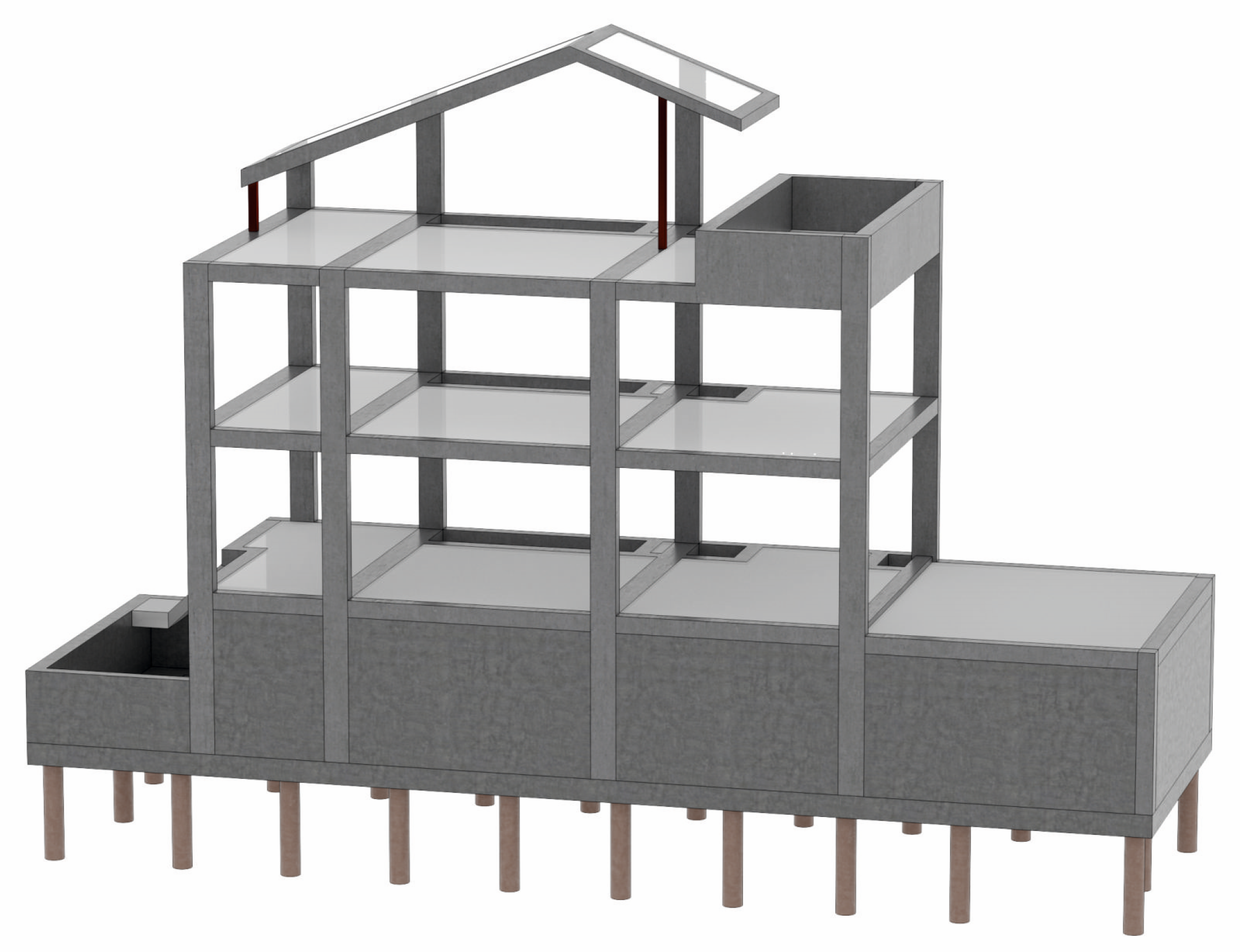
Here, an adaptive model based on the ANP has been proposed to consider the relationships between the alternatives and the different criteria with quantitative variables, generating an entire network that considers all the influences between them when making the final decision. This method is applied to the sustainability performance of four different design options for the structure of a residential building over its life cycle. Finally, an improved version of the ELECTRE I [30] method is used in the fuzzy intermediate values environment, combining the weights of the AHP and ANP groups with the so-called ELECTRE IS [31].

The remainder of the paper is structured as follows: Section 2 develops the methodology with the different techniques applied in the calculation procedure. Section 3 presents a sustainable design decision problem as a case study to apply the proposed ANP and ELECTRE IS adaptation. Section 4 collects the results and their respective analysis; a sensitivity study with other models is also included here. Finally, Section 5 concludes the research and presents proposals for future work.

2. Materials and Methods

2.1. Fundamentals of the Analytic Hierarchical Process (AHP)

The classical AHP was born out of the need to solve specific decision problems in the U.S. Department of Defense in the late 1970s. This MCDM method, developed by Professor Thomas L. Saaty, ended up extending its application to almost all fields and complex situations that required a decision support tool. The methodology helps to select between alternatives based on a series of selection variables (criteria), usually hierarchical and often in conflict with each other. The structure is hierarchized top-down, starting from the final objective, the criteria, sub-criteria, and indicators (if applicable), and, finally, the alternatives to be compared. A fundamental aspect of the method is the adequate definition of the variables to be considered relevant and mutually exclusive (independent of each other).

The mechanics of the method are based on the realization of pairwise comparison matrices at each hierarchical level, where the DM expresses the relative priority of one concept over another and the intensity of this preference. These comparisons are scored according to the Saaty Fundamental Scale [32], which uses the principle of the Weber–Fechner. As the relationship between stimulus and perception corresponds to a logarithmic scale, the perception evolves as an arithmetic progression if a stimulus grows in geometric progression. Thus, Saaty’s scale makes it possible to transform a set of nine definitions of qualitative relevance into quantitative values between 1 and 9. This semantic scale expresses a gradation of how important a criterion or alternative “i” is considered to another “j”, with 1 being “equally important” and 9 equivalent to “i is extremely more important than j”. As a result, the so-called decision matrix A = {a_ij} is obtained, which is a square matrix satisfying the properties of: reciprocity (if a_ij = x, then a_ji = 1/x ∀i,j∈{1, …,n}, where n is the number of criteria or alternatives to be compared); homogeneity (if i and j are of equal importance, a_ij = a_ji = 1, and a_ii = 1 ∀i∈{1, …,n}).

One of the virtues of the method is to evaluate the coherence of the decision, for which matrix A must not contain contradictions in the judgments expressed. Consistency can be measured through the consistency index (CI), defined as:

$$CI=({\lambda }_{max}-n)/\left(n-1\right)$$

(1)

where λ_max is the greatest eigenvalue and n is the dimension of the decision matrix. From the CI value obtained, a consistency ratio (CR) can be obtained as:

$$CR=CI/RI$$

(2)

where RI is the random index, which indicates the consistency of a given random matrix according to

Table 1. Random index (RI) values for a discrete set of criteria n ≤ 10.

Number of Criteria (n)	2	3	4	5	6	7	8	9	10
RI	0	0.58	0.90	1.12	1.24	1.32	1.41	1.45	1.49

. If CI is close to RI, the matrix has been completed randomly, thus expressing an absolute inconsistency in evaluating the problem to be solved. Conversely, a low consistency ratio means that the DM has a clear knowledge of the problem to be solved, being for CI = 0 a complete consistency. Inconsistency will be acceptable if the CR does not exceed the values indicated in

Table 2. Maximum consistency ratio (CR).

Matrix Size (n)	CR (%)
3	5
4	9
≥5	10

, in which case the subjective weightings would have to be revised.

Once the consistency has been verified, the weights, which represent the relative importance of each criterion or the priorities of the different alternatives concerning a given criterion, are obtained by solving the following equation:

$$A·w={\lambda }_{max}·w$$

(3)

where A is the comparison matrix, w is the eigenvector or preference vector and λ_max is the eigenvalue.

2.2. Fundamentals of the Analytical Network Process (ANP)

In an AHP-based decision model, the criteria (and sub-criteria and indicators, if applicable) and alternatives are structured hierarchically through a linear and unidirectional relationship between levels. According to Saaty [25], the ANP method allows a much broader representation of the decision problem by structuring it in the form of a network. In this model, interdependencies between all system components are possible. The independence of the elements of a higher level concerning those of a lower level is not assumed, nor is independence between elements of the same level. This allows for a non-linear structure that prioritizes elements and groups or clusters of elements better adapted to the complexity of the real world.

A network model consists of elements or nodes (mainly decision criteria and alternatives) grouped into components, groups, or clusters. The clusters are denoted by C_k (where m = 1, 2, …, m), and it is established that each cluster contains e_nk elements denoted by e_1k, e_2k, …, e_nk. An element of a cluster in the network can have one or bidirectional influence on some or all of the elements of that cluster or a different cluster belonging to the network. These relationships are feedback (between elements of the same cluster) and interdependent (between components of different clusters). In general terms, the ANP consists of two fundamental stages: the first is the structuring of the problem (construction of the network), and the second is the calculation of the priorities of the elements. However, the specific six steps for implementing the ANP are listed below:

Step 1: Model the decision problem as a network. The quality of the network depends mainly on the degree of knowledge of the problem on the part of the DM. The process begins with identifying network elements (criteria and alternatives).

Step 2: Grouping of the elements into components. The DM needs to properly define which of the above elements will be part of each cluster based on sharing some common characteristics.

Step 3: Analysis of the network of influences. Each element m_ij in the ANP matrix is filled in with values 0 or 1, where 1 means that element i is influenced by element j. It should be noted that this is not a reciprocal matrix, i.e., element i can be influenced by element j, but element j does not necessarily have to be influenced by element i. Thus, a correlation matrix is obtained, which is called the influential supermatrix.

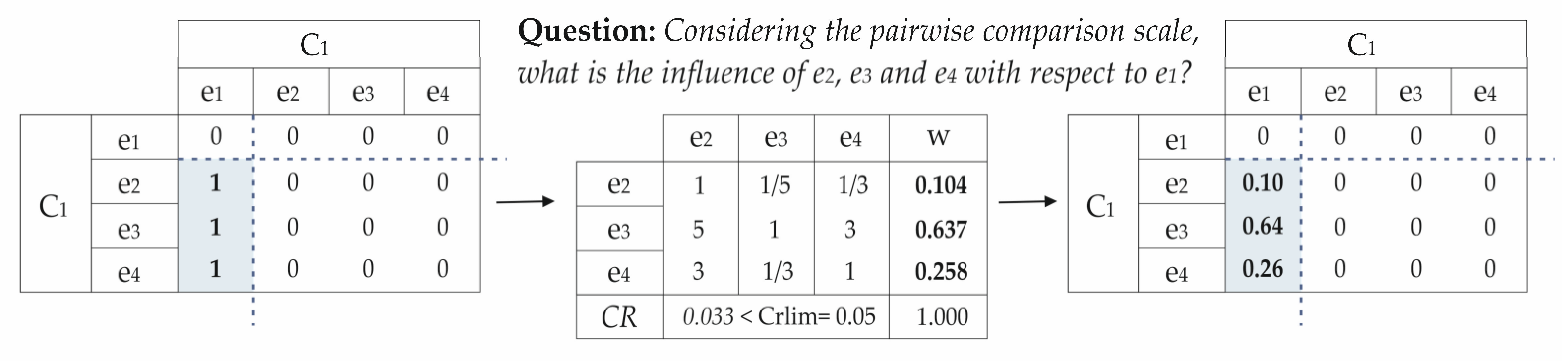
Step 4: Calculation of priorities between elements. For each cluster, only the non-zero components of the matrix will be considered. There are as many pairwise comparison matrices between elements associated with a network element as groups of elements belonging to the same cluster that influence that element. This influence is obtained by the conventional AHP method, using Saaty’s fundamental scale to complete the entries of the paired comparison matrices. Let us assume as an example that elements e₂, e₃, and e₄, both belonging to cluster C₁, have an influence on element e₁ (Figure 1). A simple AHP model will be constructed to determine how much influence each of the three elements has on e₁.

By performing this process with each element of the influential supermatrix, the so-called unweighted supermatrix is constructed. The elements that indicated the existence of influence with a “1” are now replaced by the quantification of such influence. The inputs collect the weights of the relative influence of the elements located in the rows of the matrix on the elements located in the columns, as shown in Figure 1.

Step 5: Calculation of priorities between clusters. It should be noted that the matrix of the previous step is not stochastic, i.e., its columns do not add up to 1. For the unweighted supermatrix to be stochastic, the elements of each cluster will be multiplied by the weight of each cluster (considering both criteria and alternative clusters). A pairwise inter-cluster comparison matrix associated with a given network cluster is one whose rows and columns consist of all the clusters in the network that influence that given component. There are as many paired comparison matrices between clusters in the model as groups of clusters influencing any given cluster in the network. These weights are again obtained using a conventional AHP procedure. The resulting stochastic supermatrix is then called the weighted supermatrix.

Step 6: Determine the criteria weights and the preferred alternatives. The stochastic weighted supermatrix is raised to successive powers until its entries converge and remain stable. Such matrix is called the limiting supermatrix, and all its columns are equal. If you want to know the final ranking of the alternatives, look at the entries in any column of the limiting supermatrix corresponding to the rows associated with the alternatives. These values will not sum to one but can be normalized by dividing each value by the sum of the column.

2.3. Group Aggregation Technique

When several experts participate in the decision-making problem, the question arises of how to include in the process the preferences of each expert based on their relevance within the group. The calculation of expert voting power adopted in this study is based on the recent paper by Sodenkamp et al. [33], which proposes determining each expert’s relevance based on the neutrosophic triad (truth, indeterminacy, and falsity). A simplified version of the fuzzy function [34] is employed here. Two parameters are set to determine the voting power of each expert, namely, their competence through self-assessment and their consistency in completing the evaluation matrix. Thus, voting power (Φ_i) of expert i is calculated as the Euclidean distance from each point to the ideal point of maximum credibility 〈1, 0〉, formulated as:

$$\Phi { }_i=1-\sqrt{\left\{\left(1-{\delta }_i{}^2\right)+{\epsilon }_i{}^2\right\}/2}$$

(4)

The Delphi method evaluation technique is followed to characterize the expert panelists, which usually considers aspects such as years of professional experience, presentations at conferences, authorship of articles in peer-reviewed journals, qualifications, committee membership, etc. [35]. In this case, the degree of knowledge in specific evaluation fields is incorporated to calculate the coefficient of the voting power of each expert, following the methodology applied by Sierra et al. [36].

This approach is inspired by the technique used by the Russian State Committee for Science and Technology [37], which considers two types of parameters to determine the expert profile of the panelists, namely knowledge-oriented parameters and argumentation-oriented parameters. The knowledge-oriented parameters are based on the general knowledge of the expert, namely, years of professional experience, authorship of JCR articles, and papers presented at conferences. The higher the score on these parameters, the more critical thinking ability is revealed. The other set of parameters, those oriented to argumentation, is related to expertise in the specific fields to be evaluated, in our case, sustainability and its dimensions, construction, and multi-criteria analysis. The resulting indicator reflecting the voting power of each expert is then obtained as the average of each parameter. Based on the above, the credibility of each expert is determined as follows:

$${\delta }_i=0.6\left(\frac{P{A}_i}{max\left\{P{A}_k\right\}}+\frac{S{E}_i}{max\left\{S{E}_k\right\}}+\frac{R{J}_i}{max\left\{R{J}_k\right\}}+\frac{R{P}_i}{max\left\{R{P}_k\right\}} /4\right)+0.4\left({\displaystyle \sum }_{m=1}^{n}K{F}_{m,i}/n\right)$$

(5)

where PA_i indicates the years as an active professional of i-th expert; SE_i counts the number of years of experience in sustainable issues; RJ_i and RP_i quantify the scientific production as primary author in articles for journals with JCR impact factor and papers in international congresses, respectively; max{PA_k}, max{SE_k}, max{RJ_k} and max{RP_k} are the maximum of these attributes among the k-experts. The KF_m,i parameters integrate the expert’s knowledge in several disciplines associated with the decision-making problem. In this case, n = 5 fields have been chosen, representing the level of competence in construction and civil engineering, economic appraisals, environmental assessment, social analysis, and MCDM methods.

At last, the inconsistency (ε_i) is evaluated from the inconsistencies derived from each of their pairwise comparisons performed by each expert in the AHP group and is calculated on a single matrix as:

$${\epsilon }_i=C{R}_i/C{R}_{lim}$$

(6)

In addition, for each expert of the ANP group, it is calculated on the total number of matrices to be completed as follows:

$${\epsilon }_i=\sum \left(C{R}_{ij}/C{R}_{lim,j}\right)/M_i$$

(7)

where CR_i is the consistency ratio of the i-th expert on the comparison matrix filled in a classical AHP decision process for the set of criteria; CR_ij is the consistency ratio of the i-th expert regarding the j-th comparison matrix filled along the ANP decision process; CR_lim and CR_lim,j are the limiting consistency ratios in the AHP and ANP matrices, respectively, depending on the number of elements to compare according to Table 2; M_i represents the total number of matrices filled in by expert i belonging to the ANP group.

Once the weights (w_ij) for each criterion j have been determined for each i-th expert along with their voting power (Φ_i), the final AHP/ANP group weights of the k-experts are obtained for each criterion as follows:

$$W_i=\frac{{{\displaystyle \sum }}_k{w}_{ij}·{\Phi }_i}{{{\displaystyle \sum }}_k{\Phi }_i}$$

(8)

2.4. Outranking Methods

The last part of the methodology consists of aggregating the one-dimensional life cycle performance results to evaluate each alternative from a three-dimensional approach to sustainability that allows ranking them in order of preference. In addition to the ranking obtained with the pairwise comparison MCDM methods, the criteria weights obtained by AHP and ANP are combined with an outranking MCDM method to compare the results.

These methods establish a ranking order among a discrete set of alternatives in which each solution shows a degree of dominance over the others about a criterion. Any preference structure can be defined using an outranking relation, establishing the conditions for alternative A to overcome alternative B. Thus, alternative A surpasses (S) alternative B if the DM prefers it to B or shows indifference (I) between the two. Among the methods that strictly apply this definition of outranking relation, those of the ELECTRE family stand out, considering ELECTRE I was historically the first outranking method [30]. They can deal with incomplete and fuzzy information and allow alternatives to be ranked according to the preference relation between them.

ELECTRE IS

The modeling of the decision maker’s preferences in the ELECTRE IS version [31] is less rigid than in ELECTRE I since the following argument is supported: if the difference between the valuations of the alternatives A and B is minimal, will the DM continue to prefer one of them?

Therefore, this method improves the previous version by incorporating fuzzy overclassification logic through pseudo-criteria, allowing the DM to choose decision parameters as intervals instead of fixed (true) values. The steps of ELECTRE IS and calculations are presented below.

The first step is to obtain the optimum value for each criterion among all the alternatives to be evaluated. It will correspond to the highest or lowest score depending on whether the variable is to be maximized or minimized, respectively.

$$Z_{ij+}=r_{ij}/ma{x}_j{r}_{ij}$$

(9)

$$Z_{ij-}=r_{ij}/mi{n}_j{r}_{ij}$$

(10)

The pseudo-criterion is a function in which the preference between two alternatives is characterized by two non-zero thresholds: one of indifference q_j and one of strict preference p_j (p_j ≥ q_j) for a specific criterion j.

The indifference threshold may reflect the minimum uncertainty limit in the data, while the preference threshold may report the maximum uncertainty limit. Note that when p_j = q_j, a pseudo-criterion becomes a true criterion. The concordance index C_j (A,B), which states to what extent alternative A is at least as good as alternative B for criterion Z_j, will be a value between 0 and 1 which is defined as:

$$C_{j }\left(A_{ },B_{ }\right)=\left\{\begin{array}{cc}0& p_j<Z_{ j}\left(B\right) –Z_{ j}\left(A\right),\\ \frac{Z_j\left(A_{ }\right)+p_j-Z_j\left(B\right)}{p_j-q_j}& q_j<Z_{ j}\left(B\right) –Z_{ j}\left(A\right)\le p_{j }\\ 1& Z_{ j}\left(B\right) –Z_{ j}\left(A\right)\le q_j\end{array}\right.\left(linear interpolation\right)$$

(11)

The concordance index values are incorporated into the concordance matrix by aggregating the DM weights as follows:

$$C_{ij}={\displaystyle \sum }_{j=1}^n{w}_j·C_j\left(A,B\right)/{\displaystyle \sum }_{j=1}^n{w}_j$$

(12)

Correlatively to the preference and indifference thresholds, it also introduces an additional threshold, called the veto threshold. It reinforces support when it diminishes the importance of the coalition with which it agrees, making it possible to build authentic ex æquo classes (ties). The no veto condition can be formulated as:

$$Z_j\left(A\right)+v_j\left(Z_j\left(A\right)\right)\ge Z_j\left(B\right)+q_j\left(Z_j\left(B\right)\right){\eta }_j$$

(13)

$${\eta }_i=\frac{1-C_{ij }-w_{j }}{1-c^{*}-w_{j }}$$

(14)

where v_j is the veto threshold concerning the j criterion (v_j ≥ p_j ≥ q_j); Z_j is the normalized score for each criterion as a function of each alternative; η_j is the importance coefficient; C_ij corresponds to the concordance index of each pair of alternatives; and c* is the concordance threshold defined as the next value greater than or equal to the average in the scores of the concordance matrix.

Finally, the A_i alternative outperforms A_k provided the following conditions are met:

• Concordance criteria: C_j (A,B) ≥ c*;
• Discrepancy criterion: There is no criterion j such that Z_j (B) − Z_j (A) > v_j;

that is, Z_j (A) − Z_j (B) ≥ −v_j for all the criteria.

3. Case Study

3.1. Description of the Functional Unit and Design Alternatives

The methodology described above is then applied to a multi-criteria decision-making problem, comparing the evaluation of four different construction alternatives to determine the suitability of the best structural design in terms of sustainability for a detached house built in Jaén (Spain). From the geotechnical point of view, this is a building on very conflictive soil, with clays of low bearing capacity that are highly expansive and chemically aggressive due to their sulfate content.

A baseline design (REF hereafter) will serve as the reference solution for the study (Figure 2). It consists of conventional 25 MPa reinforced concrete slabs and columns. The partition walls between dwellings and the facades are constructed with double brick sheets and mineral wool interior thermal insulation. The substructure comprises a deep foundation of drilled piles without shafts under foundation beams, using 35 MPa and 30 MPa concrete, respectively, due to the exposure environment.

The second design alternative (hereafter, ALC) is based on industrialized construction, with a semi-dry assembly of autoclaved aerated concrete structural elements (a “YTONG” system), consisting of prefabricated reinforced slabs and confined masonry block walls.

The third option to be evaluated (hereafter TWT) is based on twin-wall technology (an “ELESDOPA” system) with transverse connectors, which maximizes the inertia of the reinforced concrete H-section while reducing material costs. The space between the twin walls is filled with rigid thermal insulation, which lightens the section and serves as lost formwork.

The last construction alternative (hereafter referred to as LSV) consists of lightweight slabs voided with recycled plastic cavities (a “UNIDOME” system). Efficiency is achieved by eliminating material with only an insignificant load-bearing function. In this way, savings are sought in concrete and steel reinforcement consumption. The weight reduction also makes it possible to realize slimmer building structures.

For the results of the life cycle cost analysis (LCCA), the environmental life cycle assessment (LCA), and the social life cycle assessment (SLCA) to be comparable, ISO 14040 requires that they relate to the same functional unit. In the evaluation of the environmental, economic, and social life cycle impacts of each of the described design alternatives, the functional unit considered is a single-family row house of 384.69 m² built, located in Jaén (Spain), with a basement and two floors occupying a plot area of 20.00 m × 6.20 m. Construction, maintenance, and demolition activities are considered a useful life of 50 years, as established by the Spanish Structural Code [38]. Maintenance is assumed to increase progressively every ten years as the building deteriorates closer to the end-of-life (EoL) stage. Except for the REF option, the rest of the design alternatives consider manufacturing concrete with a percentage of no more than 20% recycled aggregates.

3.2. Impact Assessment

For the evaluation of the sustainability of each alternative throughout its life cycle, a set of seven criteria are considered, each of which corresponds to a specific type of impact related to each of the three dimensions of sustainability.

Table 3. Sustainability criteria relevant to a single-family housing structure.

Dimension	Criterion	Summary of Impact	Impact Assessment
Economy	C1−Construction costs	Costs associated with the design stage, the construction and the management of waste materials, including the costs derived from transportation activities and the various authorization fees.	Measured in €/m2. No normalization required.
	C2−Maintenance and EoL costs	Costs associated with the service life stage, from prevention and decennial maintenance to the EoL phase, which includes the activities of complete demolition of the structure and waste management, transportation costs and permitting fees.	Measured in €/m2. Weightings for each ten-year maintenance due to cadastral depreciation. Future costs discounted assuming d = 2%.
Environment	C3−Environmental damage	Life cycle impact assessment translates emissions and resource withdrawals into a limited number of environmental impact scores using so-called characterization factors. The endpoint indicators show this impact on the environment through three higher levels of aggregation, the (1) resource scarcity, (2) damage to ecosystems and (3) damage to human health.	ReCiPe methodology. The endpoint approach combines the negative and positive impacts of the three categories to obtain an overall impact score.
Society	C4−Local community	Employment generated by activities in the manufacturing, construction, maintenance and EoL stages and the availability of materials or equipment.	Indicators based on [43] and normalization of units by value functions.
	C5−Users	It measures the safety during the use and maintenance stage regarding the risk of pathologies and the thermo-acoustic comfort provided to the user by the building envelope.	Indicators based on [43] and normalization of units by value functions.
	C6−Workers	Operator health and safety associated with the accident rate during construction and demolition activities, as well as taking into account fair wages.	Indicators based on [43] and normalization of units by value functions.
	C7−Externalities	Issues related to public commitment to short- and long-term sustainability stem from encouraging the incorporation of modern methods of construction.	Indicators based on [43] and normalization of units by value functions.

provides the criteria involved in the assessment and a description of the impact it represents. The resulting impacts on the economy, the environment and society have been calculated for each alternative following the evaluation method proposed by Sánchez-Garrido et al. [39], sharing the same product system provided in the present case study.

Criteria C1 and C2 are related to the economic dimension of sustainability, covering the construction costs derived from the materialization of the structure and the costs associated with its maintenance and, finally, demolition.

The C3 environmental impact of the structure is evaluated using the categories on which the most widely accepted life cycle assessment methodologies are based. In this case, ReCiPe [40], which includes midpoint (problem-oriented) and endpoint (harm-oriented) impact categories, has been used. It is available to consider three different perspectives: individualistic, hierarchical, and egalitarian [41].

Finally, the social dimension of sustainability is addressed in criteria C4 to C7, defined through a hotspot analysis according to UNEP/SETAC guidelines [42] focused on social life cycle assessment.

Table 4. Impacts of each of the design options considered.

Impact Criterion	Alternatives				Units
	REF	ALC	TWT	LSV
C1	231.67	302.03	260.67	215.11	€/m2
C2	156.17	174.04	147.34	146.17	€/m2
C3	7155.23	5486.28	8022.47	5704.11	Score
C4	0.56	0.58	0.52	0.56	1
C5	0.42	0.62	0.70	0.60	1
C6	0.19	0.16	0.17	0.20	1
C7	0.31	0.52	0.76	0.55	1

¹ Heterogeneous units of social criteria normalized (0–1) with the MIVES method [6].

presents the evaluation results of the seven impact categories provided by the one-dimensional sustainability assessment through the different life cycle assessments (LCCA, LCA, and SLCA) for each design option. These values will serve as a baseline decision matrix to apply the different combinations of multi-criteria techniques proposed and obtain a holistic sustainability ranking of the alternatives from a three-dimensional perspective.

4. Results and Discussion

4.1. Network Decision-Making Model

Following the ANP methodology developed in Section 2.2, the first task to convert the decision problem into a cluster network is to build the model of relationships between criteria and alternatives. In this case study, the elements have been structured into four components or clusters relevant to decision making. The first cluster includes the four design alternatives: REF, ALC, TWT and LSV. The second cluster includes the two economic design criteria: construction and maintenance costs and lifetime costs. The third cluster corresponds to the environmental criterion that combines the three endpoint categories: resource scarcity, effect on human health and biodiversity. The last cluster contains the four social criteria categorized according to the stakeholders in Table 3: the local community, the consumer (users), the worker and society (externalities).

This clustering of elements is not rigid since it is possible to divide as many clusters as there are criteria. However, in the search for greater precision of the problem, it is prudent to seek a balance since increasing the number of relationships and criteria complicates the calculations and impairs the consistency of the DM’s judgments.

Each DM freely decides which external and internal dependency relationships it considers relevant to the problem, assigning 1 and 0 in the cells depending on whether or not the row element influences the column element. The process is repeated until all 121 possible relationships are completed. It should be noted that the DMs start from a pre-established model. The sustainability of each alternative always depends on each criterion, the value of each criterion depends on each alternative, and the alternatives do not influence each other.

Hereafter, and for simplicity, the results of the ANP matrices will be shown only for DM 1.

Table 5. Influential supermatrix from DM 1.

Clusters	Elements	Alternatives				Economy		Envir.	Society
		REF	ALC	TWT	LSV	C1	C2	C3	C4	C5	C6	C7
Alternatives	REF	0	0	0	0	1	1	1	1	1	1	1
	ALC	0	0	0	0	1	1	1	1	1	1	1
	TWT	0	0	0	0	1	1	1	1	1	1	1
	LSV	0	0	0	0	1	1	1	1	1	1	1
Economy	C1 1	1	1	1	1	0	1	0	0	1	1	0
	C2 1	1	1	1	1	0	0	0	0	1	1	0
Environment	C3 1	1	1	1	1	1	1	0	0	0	0	0
Society	C4 1	1	1	1	1	1	1	0	0	0	1	0
	C5 1	1	1	1	1	0	1	0	1	0	0	1
	C6 1	1	1	1	1	1	0	0	0	0	0	0
	C7 1	1	1	1	1	1	1	0	0	1	1	0

¹ C1 = construction costs; C2 = maintenance and EoL costs; C3 = environmental damage; C4 = local community; C5 = users; C6 = workers; C7 = public commitment to sustainability.

provides the influence supermatrix for the present problem according to the perspective of DM 1.

Once the influential supermatrix is constructed, the unweighted supermatrix of the decision-making problem is obtained (

Table 6. Unweighted supermatrix from DM 1.

Clusters	Elements	Alternatives				Economy		Envir.	Society
		REF	ALC	TWT	LSV	C1	C2	C3	C4	C5	C6	C7
Alternatives	REF	0	0	0	0	0.2679	0.2484	0.2247	0.2523	0.1795	0.2639	0.4079
	ALC	0	0	0	0	0.2055	0.2229	0.2930	0.2613	0.2650	0.2222	0.6842
	TWT	0	0	0	0	0.2381	0.2633	0.2004	0.2342	0.2991	0.2361	1.0000
	LSV	0	0	0	0	0.2885	0.2654	0.2819	0.2523	0.2564	0.2778	0.7237
Economy	C1	0.4027	0.3656	0.3611	0.4046	0	1	0	0	0.8571	0.6667	0
	C2	0.5973	0.6344	0.6389	0.5954	0	0	0	0	0.1429	0.3333	0
Environment	C3	1	1	1	1	1	1	0	0	0	0	0
Society	C4	0.3784	0.3085	0.2419	0.2932	0.3196	0.22.97	0	0	0	0.2000	0
	C5	0.2838	0.3298	0.3256	0.3141	0	0.6483	0	1	0	0	1
	C6	0.1284	0.0851	0.0791	0.1047	0.5584	0	0	0	0	0	0
	C7	0.2095	0.2766	0.3535	0.2880	0.1220	0.1220	0	0	1	0.8000	0

). Moreover, as in this case, the decision problem considers exclusively quantitative criteria; the expert only needs to complete the relationships that can occur between the criteria according to their vision of the problem. The quantification of the influence of alternatives concerning each criterion and vice versa can be deducted automatically and with proportionality rules from the values of the impacts by rows among all the alternatives or columns among all the criteria. Thus, the values of the supermatrix’s first four rows and columns can be obtained directly from the values presented in Table 4.

To achieve a stochastic and weighted supermatrix, the expert must determine the weight of the clusters (

Table 7. Weight of each cluster from DM 1.

Clusters	Elements	Alternatives				Economy		Envir.	Society
		REF	ALC	TWT	LSV	C1	C2	C3	C4	C5	C6	C7
Alternatives	REF	0				0.2452		1	0.0974
	ALC
	TWT
	LSV
Economy	C1	0.1634				0.5050		0	0.5695
	C2
Environment	C3	0.5396				0.0931		0	0
Society	C4	0.2970				0.1567		0	0.3331
	C5
	C6
	C7
CR/CRlim (%) =		15.87%				35.92%		0.00%	42.41%

) using a conventional AHP procedure. It should be noted that in these pairwise comparisons, only the clusters involved are considered, which simplifies the number of comparisons to be made, increasing the consistency of the DM and, therefore, the reliability of the decision finally taken.

To obtain the cluster weights, it was only necessary to complete three paired comparison matrices, the largest being the influence of the four clusters for economic impacts, with a size of 4 × 4. Table 7 includes the CR/CRlim ratio of each of the three paired comparison matrices to measure the consistency derived from judgments made by the DM in completing them. From the weights of each cluster, the weighted supermatrix can be derived, although it is not yet stochastic, i.e., the columns do not sum to 1. The previous supermatrix must be transformed into a stochastic weighted supermatrix (

Table 8. Stochastic weighted supermatrix from DM 1.

Clusters	Elements	Alternatives				Economy		Envir.	Society
		REF	ALC	TWT	LSV	C1	C2	C3	C4	C5	C6	C7
Alternatives	REF	0	0	0	0	0.1327	0.0609	0.2247	0.0571	0.0175	0.0257	0.0654
	ALC	0	0	0	0	0.1018	0.0546	0.2930	0.0591	0.0258	0.0216	0.1097
	TWT	0	0	0	0	0.1179	0.0646	0.2004	0.0530	0.0291	0.0230	0.1604
	LSV	0	0	0	0	0.1429	0.0651	0.2819	0.0571	0.0250	0.0271	0.1161
Economy	C1	0.0658	0.0597	0.0590	0.0661	0	0.5050	0	0	0.4882	0.3797	0
	C2	0.0976	0.1037	0.1044	0.0973	0	0	0	0	0.0814	0.1898	0
Environment	C3	0.5396	0.5396	0.5396	0.5396	0.1882	0.0931	0	0	0	0	0
Society	C4	0.1124	0.0916	0.0718	0.0871	0.1012	0.0360	0	0	0	0.0666	0
	C5	0.0843	0.0979	0.0967	0.0933	0	0.1016	0	0.7738	0	0	0.5484
	C6	0.0381	0.0253	0.0235	0.0311	0.1767	0	0	0	0	0	0
	C7	0.0622	0.0821	0.1050	0.0855	0.0386	0.0191	0	0	0.3331	0.2665	0
SUM =		1	1	1	1	1	1	1	1	1	1	1

), normalizing the value of each element by the sum of its respective column.

Finally, by successively raising the stochastic weighted supermatrix, one arrives at the limiting supermatrix (

Table 9. Limiting supermatrix from DM 1, displaying the weights of each criterion and the ranking of the alternatives.

Clusters	Elements	Alternatives				Economy		Envir.	Society
		REF	ALC	TWT	LSV	C1	C2	C3	C4	C5	C6	C7
Alternatives	REF	0.0770	0.0770	0.0770	0.0770	0.0770	0.0770	0.0770	0.0770	0.0770	0.0770	0.0770
	ALC	0.0922	0.0922	0.0922	0.0922	0.0922	0.0922	0.0922	0.0922	0.0922	0.0922	0.0922
	TWT	0.0792	0.0792	0.0792	0.0792	0.0792	0.0792	0.0792	0.0792	0.0792	0.0792	0.0792
	LSV	0.0956	0.0956	0.0956	0.0956	0.0956	0.0956	0.0956	0.0956	0.0956	0.0956	0.0956
Economy	C1	0.1162	0.1162	0.1162	0.1162	0.1162	0.1162	0.1162	0.1162	0.1162	0.1162	0.1162
	C2	0.0501	0.0501	0.0501	0.0501	0.0501	0.0501	0.0501	0.0501	0.0501	0.0501	0.0501
Environment	C3	0.2122	0.2122	0.2122	0.2122	0.2122	0.2122	0.2122	0.2122	0.2122	0.2122	0.2122
Society	C4	0.0467	0.0467	0.0467	0.0467	0.0467	0.0467	0.0467	0.0467	0.0467	0.0467	0.0467
	C5	0.1182	0.1182	0.1182	0.1182	0.1182	0.1182	0.1182	0.1182	0.1182	0.1182	0.1182
	C6	0.0306	0.0306	0.0306	0.0306	0.0306	0.0306	0.0306	0.0306	0.0306	0.0306	0.0306
	C7	0.0818	0.0818	0.0818	0.0818	0.0818	0.0818	0.0818	0.0818	0.0818	0.0818	0.0818

). The power to which the previous supermatrix should be raised is ideally infinite. Convergence is usually found depending on the problem, for power value around 10. In this case, only seven products have been necessary to obtain an accuracy equaling up to four decimal places.

From this matrix, the weights of each criterion according to the view of the problem by the expert involved can be derived from rows 5 to 11, once normalized. On the other hand, the values of the first four rows provide the ranking of the alternatives according to the judgments made by the DM throughout the process described. Once the values are normalized, the preferred alternative for DM 1 is LVS with 27.8% relevance, followed by ALC with 26.8%, TWT with 23.0%, and finally, the baseline option REF with 22.8% weight.

4.2. ANP vs. AHP Results Comparison

If the same decision-making problem had been approached using the conventional AHP method to obtain the weights of n = 7 criteria, each expert would have had to complete a paired matrix of size 7 × 7. This means making only n(n − 1)/2 = 21 comparisons since, without accounting for the diagonal, the reciprocal values are always the inverse to guarantee the bidirectionality axiom. This AHP matrix for DM 1 is shown in

Table A1. AHP paired comparison matrix for DM 1.

(aij)	C1	C2	C3	C4	C5	C6	C7	=∏aij(1/n)	w
C1	1	6	1/3	4	2	3	8	2.340	0.241
C2	1/6	1	1/7	1	1/3	1	2	0.553	0.057
C3	3	7	1	5	4	3	7	3.661	0.377
C4	1/4	1	1/5	1	1/3	4	2	0.750	0.077
C5	1/2	3	1/4	3	1	3	5	1.497	0.154
C6	1/3	1	1/3	1/4	1/3	1	3	0.599	0.062
C7	1/8	1/2	1/7	1/2	1/5	1/3	1	0.313	0.032
wt	0.241	0.057	0.377	0.077	0.154	0.062	0.032	9.715	1
CI = 0.092/CR = 0.07/CRlim = 0.01

(see Appendix A). The value of the consistency ratio of this AHP matrix is CR = 0.07, which is 70% of CR_lim = 10% for comparison matrices of size 7 × 7. The number of AHP judgments is far less than those required to complete a conventional ANP, which for this particular decision problem would require a total of 282, accounting for the network of influences, the priorities between elements and the inter-cluster priorities.

The adaptive ANP model presented in this paper, being a pre-set and self-complete system based on quantitative variables, as explained in Section 4.1, only requires the expert to perform 21 criterion comparisons distributed among 8 matrices of dimension no greater than 4 × 4. This represents a 92.5% reduction in the comparisons that the DM would face in the classic ANP model. However, as explained in Section 2.1, this simplicity has its limitations. AHP is unidirectional, which means that judgments regarding the priorities of the hierarchy elements do not depend on those of the lower level. This hypothesis is refutable when there is a dependence on the importance of an objective on the lower level, as occurs in ANP. Finally, the results of each DM will be aggregated into a final group preference with the resulting ranking for both criteria and alternatives.

Table A2. Characterization and voting power of the experts of the AHP/ANP group.

Expert Profile Parameterization	Feature	DM1	DM2	DM3	DM4
Expertise
Years as an active professional	PAk	20	9	20	33
Years of experience in sustainable issues	SEk	3	7	2	17
Knowledge in field
Construction engineering	KF1	5	5	2	4
Environmental issues	KF2	2	3	2	4
Economic issues	KF3	4	4	4	4
Social issues	KF4	3	3	2	3
MCDM issues	KF5	4	4	0	5
Research work
Main author of JCR research articles	RJk	4	9	12	14
Primary author in conferences papers	RPk	7	13	9	72
Expert’s credibility	δ DMk	0.463	0.530	0.416	0.920
Expert’s incoherency (AHP)	ε DMk	0.700	0.612	0.654	0.627
Expert’s incoherency (ANP)	ε DMk	0.264	0.451	0.406	0.448
Expert’s voting power (AHP)	Φ DMk	0.269	0.361	0.255	0.549
Expert’s voting power (ANP)	Φ DMk	0.431	0.432	0.349	0.673

(see Appendix A) presents the characterization of each DM based on the knowledge- and argumentation-oriented parameters described in Section 2.3. Note that all the expert’s parameters are common for the AHP and ANP method except for the inconsistency (ε) since the number and dimension of the matrices to be filled in the two procedures are different. As a consequence of the above, each expert’s voting power (Φ) is different depending on whether the AHP or ANP methodology is applied. Note that all experts gain voting power in ANP by reducing their inconsistency as a consequence of filling matrices whose maximum size is 4 × 4 instead of 7 × 7 as in AHP, thus making more consistent judgments. Specifically, DM 1 is the expert that most increases voting power by 60%. Applying Equation (8), the final weights of each criterion are obtained, using the weights of each expert together with their voting power (Φ_i).

Table A3. Comparison of the weights for the seven criteria determined through AHP and ANP.

Criteria	DM1		DM2		DM3		DM4		AHP-G 1	ANP-G 1
	AHP	ANP	AHP	ANP	AHP	ANP	AHP	ANP
(C1) Construction cost	0.241	0.177	0.049	0.068	0.340	0.085	0.184	0.087	0.188	0.103
(C2) Maintenance + EoL cost	0.057	0.076	0.142	0.072	0.091	0.072	0.055	0.092	0.083	0.080
(C3) Environmental damage	0.377	0.324	0.349	0.263	0.184	0.382	0.255	0.419	0.289	0.354
(C4) Local community	0.077	0.071	0.126	0.084	0.028	0.076	0.082	0.059	0.083	0.071
(C5) Users	0.154	0.180	0.230	0.246	0.267	0.182	0.328	0.165	0.260	0.190
(C6) Workers	0.062	0.047	0.050	0.029	0.033	0.031	0.062	0.023	0.054	0.031
(C7) Public commitment	0.032	0.125	0.054	0.237	0.057	0.172	0.034	0.155	0.043	0.170

¹ Weighting obtained according to Equation (8).

(see Appendix A) reports the results with the criteria weights at the individual and group level for both AHP and ANP. Considering the above, the scores of each alternative and criterion are normalized and aggregated while also considering the relevance of each DM.

Table 10. Comparison of the results of the AHP group vs. the ANP group.

Expert Group	Weights	REF	ALC	TWT	LSV	C1	C2	C3	C4	C5	C6	C7
AHP-G	Alternatives	0.224	0.255	0.250	0.271	-	-	-	-	-	-	-
	Criteria	-	-	-	-	0.188	0.083	0.289	0.083	0.260	0.054	0.043
ANP-G	Alternatives	0.217	0.269	0.239	0.275	-	-	-	-	-	-	-
	Criteria	-	-	-	-	0.103	0.080	0.354	0.071	0.190	0.031	0.170

presents the final aggregated ranking with the criteria weights and alternatives after applying AHP and ANP as MCDM methods.

Observing the weight of each design option obtained through the AHP and ANP methods, the results are practically equivalent. Hence, their preferences coincide regarding the ranking of the alternatives: LSV > ALC > TWT > REF.

Figure 3 includes for each criterion (C1 to C7) the resulting weights decided by the AHP and ANP groups, together with the 5th and 95th percentiles between the corresponding individual weight assignments among the experts constituting each group. Although criteria C2 to C6 show a good fit with respect to the mean, there is a significant increase in the dispersion of results in the extreme criteria, namely economic C1 and social C7. The relative standard deviation (RSD) is calculated for each criterion to measure the observed dispersion. The RSD is the ratio of the standard deviation to the mean between the set of reference weights and percentiles for the criteria weights in AHP and ANP. As shown in the curves in Figure 3, criterion C7 has the highest RSD with 71.85%, followed by criterion C1 with 63.39%. In particular, criterion C7 covers social issues related to a public commitment to sustainability. Not surprisingly, this is the only social impact qualitatively obtained through semantic questionnaires, although it was later normalized into quantitative scores, as shown in Table 4.

4.3. Results Combining the Criteria Weights of the AHP and ANP Groups with ELECTRE IS

The last step that closes the proposed methodology consists of checking the robustness of the model and comparing the results obtained so far using AHP and ANP as MCDM methods. The weights obtained above for the criteria (Table 10) are combined with an outranking MCDM technique to aggregate the seven different impact categories (Table 4) into a sustainability ranking of the four alternatives. Specifically, an evolution of the original ELECTRE I, the ELECTRE IS, is used. ELECTRE IS offers an advantage as a decision support technique. This method incorporates fuzzy sets of intermediate values and uncertain environments, which, when properly combined with an analytical network structure, is an ideal option for solving practical problems of a more realistic nature, such as sustainability.

Table 11. Normalized decision matrix on impact assessment results and pseudo-criteria common to AHP and ANP-ELECTRE IS.

Criteria	Weights		Preference Threshold	Indifference Threshold	Veto Threshold	Alt. 1	Alt. 2	Alt. 3	Alt. 4
	AHP-G	ANP-G	vi ≥ pi ≥ qi			REF	ALC	TWT	LSV
			pi	qi	vi
C1−	0.188	0.103	1.068	0.712	1.424	9.285	7.122	8.252	10
C2−	0.083	0.080	1.260	0.840	1.680	9.360	8.399	9.921	10
C3−	0.289	0.354	1.026	0.684	1.368	7.668	10	6.839	9.618
C4+	0.083	0.071	1.345	0.897	1.793	9.655	10	8.966	9.655
C5+	0.260	0.190	0.900	0.600	1.200	6.000	8.857	10	8.571
C6+	0.054	0.031	1.200	0.800	1.600	9.500	8.000	8.500	10
C7+	0.043	0.170	0	0	0.816	4.079	6.842	10	7.237

shows the relevance that the AHP and ANP groups have decided for each criterion, the thresholds used as pseudo-criteria and the seven impact scores once normalized for each alternative. Now the comparison is not limited to the evaluation of each alternative concerning the criteria defined in the model but also includes the indifference (q), preference (p), and veto (v) thresholds. Here, 10%, 15%, and 20% of the minimum value have been set for each criterion, respectively. Note that C7 is the only criterion considered with real values instead of intervals (q = p = 0) because it comes from the normalization of social impacts obtained through qualitative scales [39].

Table 12. Results of sustainability assessment according to AHP and ANP combined with ELECTRE IS.

Sustainability	AHP-ELECTRE IS					ANP-ELECTRE IS
	0.65	Global Concordance Index (c*)				0.64	Global Concordance Index (c*)
Alternatives	Σ rows	Outranking relation				Σ rows	Outranking relation
		REF	ALC	TWT	LSV		REF	ALC	TWT	LSV
REF	1	−	0	1	0	1	−	0	1	0
ALC	1	1	−	0	0	1	1	−	0	0
TWT	2	1	1	−	0	1	1	0	−	0
LSV	3	1	1	1	−	3	1	1	1	−
	Σ columns	3	2	2	0	Σ columns	3	1	2	0
Ranking	Level	IV	III	II	I	Level	IV	II	III	I

includes the results with the rankings of alternatives in the AHP and ANP with ELECTRE IS combinations. In both cases, LSV and REF coincide as the best and worst sustainable design options. Figure 4 reveals an alternation between the second and third positions of LAC and TWT, depending on whether the ANP weights or vice versa have been combined with AHP. In any case, the ranking fully coincides when the ANP influence network is taken into account, either as an integral procedure of MCDM or by combining the weights of its variables with ELECTRE IS. Compared to the AHP process, ANP allows us to go a step further in modeling the complex relationships between the different criteria, making it possible for the expert to reflect their vision of the problem more flexibly and accurately, thus increasing the reliability of the final decision.

4.4. Validation of Results and Sensitivity Analysis

4.4.1. Sensitivity According to the Subjective Weight Assignment Method

A comparison is made between the weights obtained with the AHP and ANP models and those resulting from applying the best-worst method (BWM) [44,45] and the full consistency method (FUCOM) [46]. These two techniques have been chosen from the subjective methods available to determine the weighting coefficient. In addition, BWM and FUCOM are based on the concept of pairwise comparison of criteria and the consistency of such comparisons, sharing principles with AHP and ANP.

Based on the results presented (see

Table 13. Criteria subjective weighting using BWM, FUCOM, AHP, and ANP methods.

Sustainability Dimension		Economy		Environ.	Society
Method	Weights	C1	C2	C3	C4	C5	C6	C7
BWM Ksi = 0.067	Criteria	0.144	0.072	0.217	0.087	0.365	0.072	0.042
	Cluster	0.217		0.217	0.567
FUCOM DFC(χ) = 0.000	Criteria	0.162	0.081	0.323	0.065	0.269	0.054	0.046
	Cluster	0.243		0.323	0.434
AHP CR = 0.040	Criteria	0.188	0.083	0.289	0.083	0.260	0.054	0.043
	Cluster	0.272		0.289	0.439
ANP CR = 0.0259	Criteria	0.103	0.080	0.354	0.071	0.190	0.031	0.170
	Cluster	0.183		0.354	0.462

), comparing the weights of the clusters (equivalent to each of the dimensions of sustainability) that encompass the criteria obtained by the four methods shows similar results. The weights of the economic, environmental, and social clusters represent a standard deviation of only 3.8%, 5.8%, and 6.17%, respectively, among the four methods. However, with the more specific weightings for each criterion, some variations become very significant, especially in the social criteria, such as C7. The reason is that social evaluation is more sensitive to the experts’ subjectivity. Thus, the methods used are equally valid for capturing the experts’ overall view of the problem. However, at the criteria level, the differences are more pronounced. Specifically, within the social cluster, there has been a redistribution of weights between criteria assigning 17% to C7 according to the network of influences of the ANP, in contrast to 4% according to the hierarchical linearity of the AHP, BWM and FUCOM methods.

It should be noted that there is a significant difference in terms of consistency between the four methodologies. BWM has the advantage of requiring only 2n − 3 comparisons versus n(n − 1)/2 comparisons for the AHP, with a K_si coefficient of 0.067 showing a high degree of reliability in the results; the closer to zero, the better. For FUCOM, the degree of DFC (deviation from total consistency) is the deviation value of the obtained weight coefficients concerning the estimated relative priorities of the criteria. In addition, the DFC also confirms the reliability of the obtained criteria weights. The maximum consistency requirement is met if the DFC is zero, as in our case, where χ=0.00. However, both methods are based on a linear hierarchy process, losing accuracy when considering feedback and interdependent effects between elements and components of the ANP method.

Considering the CR/CR_lim parameter, the uncertainty is more significant with AHP-G (64.2%) than with ANP-G (39.8%), so it can be stated that the latter results are more reliable. Therefore, the ANP model, adapted for quantitative variables, seems more suitable to accurately reflect the experts’ opinion on the decision problem related to sustainability.

4.4.2. A Comparative Analysis of the Results with Other MCDM Methods

Once the ANP group weights have been validated, they will be combined with other well-known MCDM methods to compare the ranking with the proposed hybrid ANP-ELECTRE IS model. Four techniques have been applied, namely SAW (Simple Additive Weighting), COPRAS (COmplex PRoportional Assessment), TOPSIS (Technique for Order Preference by Similarity to an Ideal Solution), and VIKOR (multi-criteria optimization and compromise solution).

The ranking results obtained by these methods (Figure 5) show no differences in the ranking concerning the original model from a strictly mathematical point of view. However, with the application of SAW, the ALC and TWT alternatives closely dispute the second and third positions, even overlapping when COPRAS is applied. In any case, the best and worst alternatives are clearly defined and coincide in all cases. Thus, it can be stated that the results obtained with ANP-ELECTRE IS do not deviate from the results determined with the other MCDM methods.

4.4.3. Sensitivity to the Change of Coefficients in the Criteria Weights

After validation of the research results, a sensitivity analysis is performed to examine whether a change in the criteria weights varies the ranking order of the alternatives [47]. For this purpose, seven different scenarios are evaluated, in addition to the original one (

Table 14. Different weighting scenarios for aggregation in the hybrid ANP-ELECTRE IS model.

Criteria	Scenarios
	Original	S1	S2	S3	S4	S5	S6	S7
(C1) Construction cost	0.103	0.174+	0.103	0.113+	0.103	0.113+	0.103	0.113+
(C2) Maintenance+ EoL cost	0.080	0.080	0.152+	0.088+	0.080	0.088+	0.080	0.088+
(C3) Environmental damage	0.354	0.319−	0.319−	0.326−	0.319−	0.354	0.319−	0.354
(C4) Local community	0.071	0.071	0.071	0.078+	0.142+	0.078+	0.071	0.078+
(C5) Users	0.190	0.171−	0.171−	0.190	0.171−	0.162−	0.171−	0.190
(C6) Workers	0.031	0.031	0.031	0.034+	0.031	0.034+	0.103+	0.034+
(C7) Public commitment	0.170	0.153−	0.153−	0.170	0.153−	0.170	0.153−	0.142−

).

The strategy consists of choosing the n criteria as the most susceptible to change according to its subjectivity load. For example, considering C1 as the most subjective, its weight will be increased to the same extent that those criteria whose weight is more significant than 100/n (C3, C5, and C7 in this scenario) and will be reduced by −10%, leaving the rest fixed and keeping the sum of all the weights at 1. In the opposite case, as in C3, its importance will be reduced by increasing criteria C1, C2, C4, and C6 by +10%.

The results of the application of these scenarios, shown in Figure 6, show that the LSV alternative occupies first place in all cases, except in scenario S3, where there is no relationship of outranking concerning the TWT alternative. The REF alternative is always the least preferred, ranking fourth. As for ALC, this alternative ranks second in five of the eight scenarios, while the TWT alternative ranks second in three scenarios (sharing first place in scenario S3).

Figure 7 shows the Spearman rank correlations between each pair of variables, considering the original case and the seven alternative scenarios. Spearman’s correlation factor ρ is a nonparametric measure of rank correlation that determines whether there is a monotonic relationship, either linear or non-linear, between two variables. These correlation coefficients range from −1 to +1 and measure the strength of the association between the variables. If the value ρ approaches 0, the association between the two ranks is weaker. In contrast to the more common Pearson correlations, the Spearman coefficients are calculated from the order (ranks) of the data rather than the data values themselves, so they are less sensitive to outliers than the Pearson coefficients.

The results show strong correlations between the scenarios, except for S3, S4, S5, and S7, which remain positive and relatively high (0.6325). Note that between S4, S5, and S7, the correlation is 1, which means that variations in the parameters of these three scenarios influence the ranking similarly. In other words, the original scenario is sensitive to the parameters that have changed in S4, S5, and S7, which correspond to the scenarios of three of the most subjective social criteria. It is confirmed that social assessment is more sensitive to the subjectivity of the expert since it is a dimension of sustainability whose quantification is still in a very incipient development process.

5. Conclusions

Building a better world means aligning with the SDGs set for 2030. In this sense, the construction sector has a fundamental role to play, as it can be responsible for a large number of effects, both positive and negative, on the environment, the economy, and society. The sustainable design of buildings and urban districts has focused the efforts of a significant part of the scientific community. Mitigating their considerable negative impacts on the environment and boosting economic growth and social welfare are essential to achieving the sustainable future to which our society aspires. However, sustainability and construction management are complex issues involving multiple competing criteria. Moreover, the quantification of sustainability is difficult to objectify since it depends on the subjective perception of each DM and the relevance assigned to each criterion. These issues require techniques that make it possible to model the decision-making problem as closely as possible to reality, considering the interdependence and feedback relationships between the different criteria that are limited by methods such as AHP. With the ANP method, more reliable results can be obtained, but at the cost of many more questions and comparisons that further complicate the calculations by increasing the number of relationships and criteria. This means that the experts have to intervene much longer, diluting the concentration and introducing more significant uncertainties in their judgments. An ANP model adapted to quantitative units, specific to the criteria for sustainability assessments in building structures, has been calibrated to simplify this process.

This paper evaluates sustainability performance among four different structural design alternatives for a single-family dwelling over its life cycle based on various combinations between other MCDM methods of pairwise comparison and outperformance. In most cases, the preferred design option for sustainability performance is based on lightweight slabs with recycled plastic hollow corps. The results show the advantages of using ANP when the problem, such as the one at hand, can be formulated from a quantitative definition of the criteria used in the decision-making process. The model has significant advantages since it continues to identify the feedback and interdependencies in the network but greatly simplifies the computation of the network by reducing the number of questions to be answered by the experts involved in the decision process. For these cases, the ANP methodology makes it possible to automatically complete part of the clusters from the data input, which reduces the experts’ judgments and thus increases their consistency.

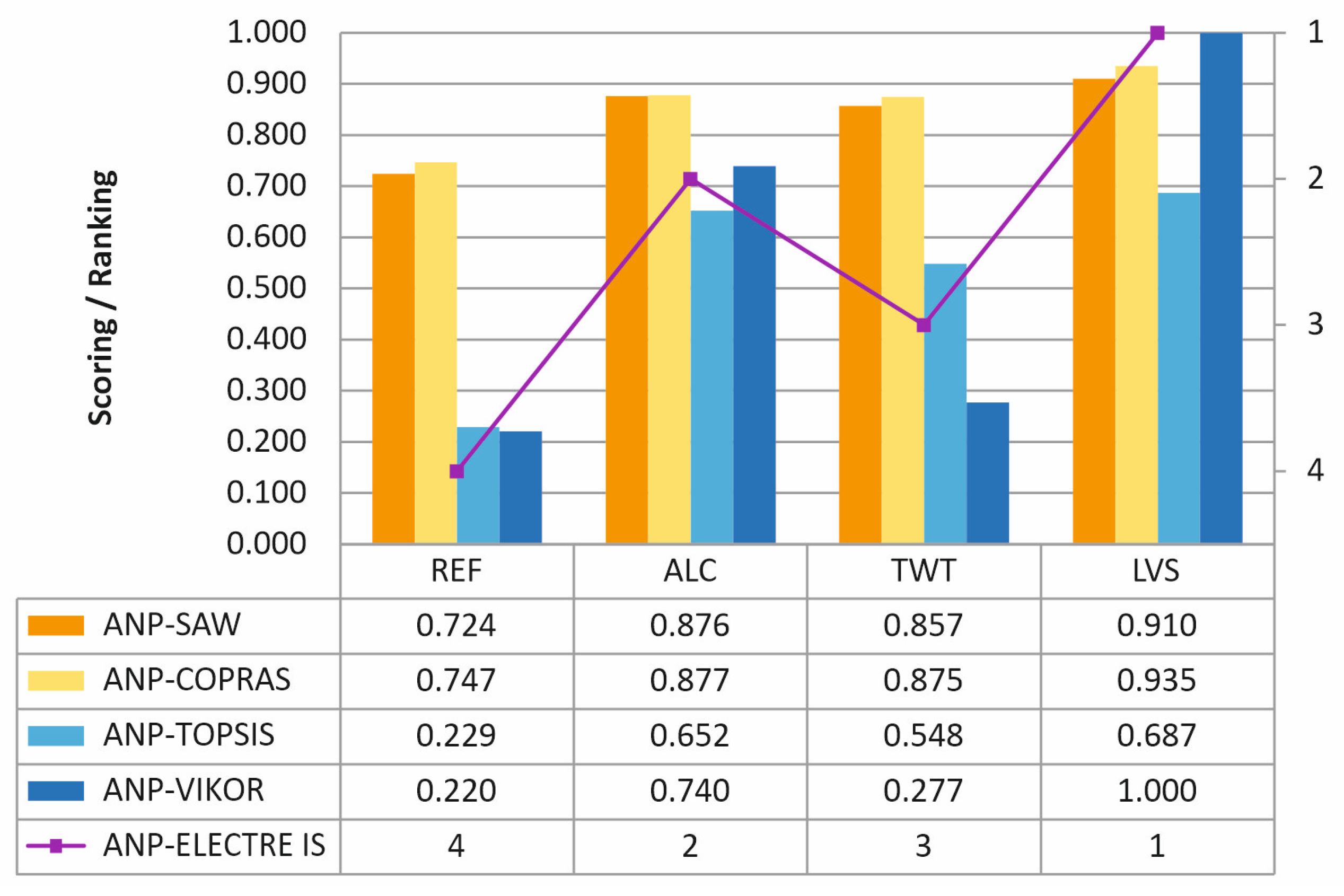
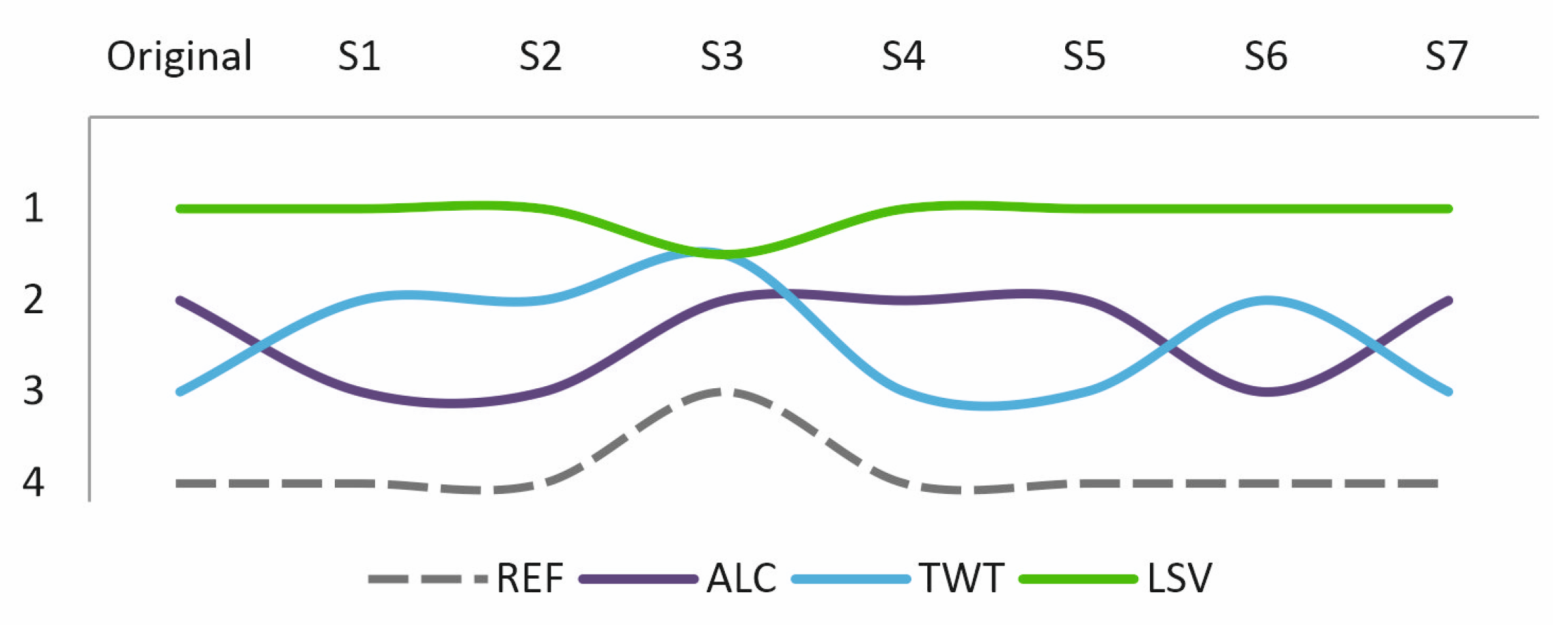
Finally, based on the weights obtained by the AHP and ANP groups, the MCDM method of outranking ELECTRE IS was applied to aggregate the seven impact categories to compare each design option through a sustainability ranking. The ELECTRE technique, specifically the IS variant, simultaneously considers the heterogeneity of the criteria ranges and the imperfect knowledge inherent in decision-making situations more similar to those of the real world. Introducing pseudo-criteria through imprecision thresholds in the data allows taking advantage of the fuzzy type overcoming relationship, which implies tuning less rigid modeling in terms of the decision maker’s preferences to obtain the best compromise solution. A sensitivity study has also been included with other techniques for obtaining subjective weights (BWM and FUCOM) and other MCDM methods (SAW, COPRAS, TOPSIS, and VIKOR).

Future lines of research will focus on two objectives. Firstly, to make the methodology as easy as possible for the DM and to further reduce the complexity of the intervention of each expert, an attempt will be made not only to simplify the process but also to avoid the size of the pairwise comparison matrices being a constraint by considering all the model elements as part of a single cluster. Secondly, minimization through neutrosophic logic of the effect of non-probabilistic uncertainties is associated with the decision maker’s ability to consistently reflect his view of the problem when making a judgment.

References

1. Cinelli, M.; Coles, M.; Kirwan, K. Analysis of the potentials of multi criteria decision analysis methods to conduct sustainability assessment. Ecol. Indic. 2014, 46, 138–148. [Google Scholar] [CrossRef]
2. The United Nations General Assembly. Resolution Adopted by the General Assembly on 25 September 2015. Transforming Our World: The 2030 Agenda for Sustainable Development—European Environment Agency. Policy Document. Available online: http://www.un.org/ga/search/view_doc.asp?symbol=A/RES/70/1&Lang=E (accessed on 11 April 2022).
3. López, C.D.; Carpio, M.; Martín-Morales, M.; Díaz López, C.; Zamorano, M. A comparative analysis of sustainable building assessment methods. Sustain. Cities Soc. 2019, 49, 101611. [Google Scholar] [CrossRef]
4. Navarro, I.J.; Yepes, V.; Martí, J.V. Sustainability assessment of concrete bridge deck designs in coastal environments using neutrosophic criteria weights. Struct. Infrastruct. Eng. 2020, 16, 949–967. [Google Scholar] [CrossRef]
5. Salameh, M.M.; Touqan, B.A.; Awad, J.; Salameh, M.M. Heritage conservation as a bridge to sustainability assessing thermal performance and the preservation of identity through heritage conservation in the Mediterranean city of Nablus. Ain Shams Eng. J. 2022, 13, 101553. [Google Scholar] [CrossRef]
6. Sánchez-Garrido, A.J.; Yepes, V. Multi-criteria assessment of alternative sustainable structures for a self-promoted, single-family home. J. Clean. Prod. 2020, 258, 120556. [Google Scholar] [CrossRef]
7. Angeles, K.; Patsialis, D.; Taflanidis, A.A.; Kijewski-Correa, T.L.; Buccellato, A.; Vardeman, C. Advancing the Design of Resilient and Sustainable Buildings: An Integrated Life-Cycle Analysis. J. Struct. Eng. 2021, 147, 04020341. [Google Scholar] [CrossRef]
8. Torres-Machí, C.; Chamorro, A.; Pellicer, E.; Yepes, V.; Videla, C. Sustainable pavement management integrating economic, technical, and environmental aspects in decision making. Transp. Res. Rec. 2015, 2523, 56–63. [Google Scholar] [CrossRef]
9. Balasbaneh, A.T.; Marsono, A.K.B. Applying multi-criteria decision-making on alternatives for earth-retaining walls: LCA, LCC, and S-LCA. Int. J. Life Cycle Assess. 2020, 25, 2140–2153. [Google Scholar] [CrossRef]
10. García, J.; Yepes, V.; Martí, J.V. A Hybrid k-Means Cuckoo Search Algorithm Applied to the Counterfort Retaining Walls Problem. Mathematics 2020, 8, 555. [Google Scholar] [CrossRef]
11. Zavadskas, E.K.; Turskis, Z.; Kildienė, S. State of art surveys of overviews on MCDM/MADM methods. Technol. Econ. Dev. Econ. 2014, 20, 165–179. [Google Scholar] [CrossRef]
12. Penadés-Plà, V.; García-Segura, T.; Martí, J.V.; Yepes, V. A review of multi-criteria decision making methods applied to the sustainable bridge design. Sustainability 2016, 8, 1295. [Google Scholar] [CrossRef]
13. Tsoukias, A. On the concept of decision aiding process: An operational perspective. Ann. Oper. Res. 2007, 154, 3–27. [Google Scholar] [CrossRef]
14. Bigaret, S.; Hodgett, R.E.; Meyer, P.; Mironova, T.; Olteanu, A.-L. Supporting the multi-criteria decision aiding process: R and the MCDA package. EURO J. Decis. Process. 2017, 5, 169–194. [Google Scholar] [CrossRef]
15. Navarro, I.J.; Yepes, V.; Martí, J.V. A review of multicriteria assessment techniques applied to sustainable infrastructure design. Adv. Civ. Eng. 2019, 2019, 6134803. [Google Scholar] [CrossRef]
16. Zhu, X.; Meng, X.; Zhang, M. Application of multiple criteria decision making methods in construction: A systematic literature review. J. Civ. Eng. Manag. 2021, 27, 372–403. [Google Scholar] [CrossRef]
17. Saaty, T.L. A scaling method for priorities in hierarchical structures. J. Math. Psychol. 1977, 15, 234–281. [Google Scholar] [CrossRef]
18. Dong, Q.; Saaty, T.L. An analytic hierarchy process model of group consensus. J. Syst. Sci. Syst. Eng. 2014, 23, 362–374. [Google Scholar] [CrossRef]
19. Saaty, T.L. Axiomatic Foundation of the Analytic Hierarchy Process. Manag. Sci. 1986, 32, 841–855. [Google Scholar] [CrossRef]
20. Zadeh, L. Outline of a new approach to the analysis of complex systems and decision processes. IEEE Trans. Syst. Man Cybern. 1973, SMC-3, 28–44. [Google Scholar] [CrossRef]
21. Shapiro, A.F.; Koissi, M.-C. Fuzzy logic modifications of the Analytic Hierarchy Process. Insur. Math. Econ. 2017, 75, 189–202. [Google Scholar] [CrossRef]
22. Ren, P.; Xu, Z.; Liao, H. Intuitionistic multiplicative analytic hierarchy process in group decision making. Comput. Ind. Eng. 2016, 101, 513–524. [Google Scholar] [CrossRef]
23. Sánchez-Garrido, A.J.; Navarro, I.J.; Yepes, V. Neutrosophic multi-criteria evaluation of sustainable alternatives for the structure of single-family homes. Environ. Impact Assess. Rev. 2021, 89, 106572. [Google Scholar] [CrossRef]
24. Navarro, I.J.; Martí, J.V.; Yepes, V. Neutrosophic Completion Technique for Incomplete Higher-Order AHP Comparison Matrices. Mathematics 2021, 9, 496. [Google Scholar] [CrossRef]
25. Saaty, T.L. Decision Making with Dependence and Feedback: The Analytic Network Process; RWS Publications: Pittsburgh, PA, USA, 1996. [Google Scholar]
26. Ocampo, L.; Ocampo, C.O. A robust evaluation of sustainability initiatives with analytic network process (ANP). Int. J. Oper. Prod. Manag. 2015, 3, 123–133. [Google Scholar] [CrossRef]
27. Mavi, R.K.; Standing, C. Critical success factors of sustainable project management in construction: A fuzzy DEMATEL-ANP approach. J. Clean. Prod. 2018, 194, 751–765. [Google Scholar] [CrossRef]
28. Xu, J.; Li, L.; Ren, M. A Hybrid ANP Method for Evaluation of Government Data Sustainability. Sustainability 2022, 14, 884. [Google Scholar] [CrossRef]
29. Zhu, Q.; Dou, Y.; Sarkis, J. A portfolio-based analysis for green supplier management using the analytical network process. Int. J. Supply Chain. Manag. 2010, 15, 306–319. [Google Scholar] [CrossRef]
30. Roy, B. Classement et choix en présence de points de vue multiples. R.I.R.O. 1968, 2, 57–75. [Google Scholar] [CrossRef]
31. Roy, B.; Skalka, J.M. ELECTRE IS: Aspects Méthodologiques et Guide D’utilisation; Document du Lamsade, 30; Universidad Paris-Dauphine: París, France, 1984. [Google Scholar]
32. Saaty, T.L. The Analytic Hierarchy Process: Planning, Priority Setting, Resource Allocation; McGraw-Hill International Book Company: New York, NY, USA; London, UK, 1980. [Google Scholar]
33. Sodenkamp, M.A.; Tavana, M.; Di Caprio, D. An aggregation method for solving group multi-criteria decision-making problems with single-valued neutrosophic sets. Appl. Soft Comput. 2018, 71, 715–727. [Google Scholar] [CrossRef]
34. Sánchez-Garrido, A.J.; Navarro, I.J.; Yepes, V. Evaluating the sustainability of soil improvement techniques in foundation substructures. J. Clean. Prod. 2022, 351, 131463. [Google Scholar] [CrossRef]
35. Hallowell, M.R.; Gambatese, J.A. Qualitative research: Application of the delphi method to CEM research. J. Constr. Eng. Manag. 2010, 136, 99–107. [Google Scholar] [CrossRef]
36. Sierra, L.; Pellicer, E.; Yepes, V. Social Sustainability in the Lifecycle of Chilean Public Infrastructure. J. Constr. Eng. Manag. 2016, 142, 05015020. [Google Scholar] [CrossRef]
37. Oñate, N.; Ramos, L.; Díaz, A. Use of the Delphi method in forecasting: An initial experience. Econ. Planif. 1998, 3, 9–48. (In Spanish) [Google Scholar]
38. Ministry of Transport. Mobility and Urban Agenda. In Código Estructural; Ministry of Transport: Madrid, Spain, 2021; Available online: https://www.boe.es/eli/es/rd/2021/06/29/470/dof/spa/pdf (accessed on 11 April 2022).
39. Sánchez-Garrido, A.J.; Navarro, I.J.; Yepes, V. Multi-criteria decision-making applied to the sustainability of building structures based on Modern Methods of Construction. J. Clean. Prod. 2022, 330, 129724. [Google Scholar] [CrossRef]
40. Goedkoop, M.; Heijungs, R.; Huijbregts, M.; De Schryver, A.; Struijs, J.; Van Zelm, R. ReCiPe 2008: A Life Cycle Impact Assessment Method which Comprises Harmonised Category Indicators at the Midpoint and the Endpoint Level; Ministerie van Volkshuisvesting: The Hague, The Netherlands, 2009. [Google Scholar]
41. Huijbregts, M.A.J.; Steinmann, Z.J.N.; Elshout, P.M.F.; Stam, G.; Verones, F.; Vieira, M.; Zijp, M.; Hollander, A.; Van Zelm, R. ReCiPe2016: A harmonised life cycle impact assessment method at midpoint and endpoint level. Int. J. Life Cycle Assess. 2017, 22, 138–147. [Google Scholar] [CrossRef]
42. UNEP/SETAC. Guidelines for Social Life Cycle Assessment of Products; UNEP/SETAC Life-Cycle Initiative: Paris, France, 2009. [Google Scholar]
43. UNEP/SETAC. Methodological Sheets for the Subcategories of Social Life Cycle Assessment (S-LCA); United Nations Environment Programme and SETAC: Paris, France, 2013. [Google Scholar]
44. Rezaei, J. Best-worst multi-criteria decision-making method. Omega 2015, 53, 49–57. [Google Scholar] [CrossRef]
45. Rezaei, J. Best-worst multi-criteria decision-making method: Some properties and a linear model. Omega 2016, 64, 126–130. [Google Scholar] [CrossRef]
46. Pamučar, D.; Stević, Z.; Sremac, S. A New Model for Determining Weight Coefficients of Criteria in MCDM Models: Full Consistency Method (FUCOM). Symmetry 2018, 10, 393. [Google Scholar] [CrossRef]
47. Puška, A.; Nedeljković, M.; Hashemkhani Zolfani, S.; Pamučar, D. Application of Interval Fuzzy Logic in Selecting a Sustainable Supplier on the Example of Agricultural Production. Symmetry 2021, 13, 774. [Google Scholar] [CrossRef]
Figure 1. Example of determination of the influence between elements.
Mathematics 10 02009 g001
Figure 2. 3D view of the structural baseline design (REF).
Mathematics 10 02009 g002
Figure 3. Dispersion in the weightings of the criteria with AHP and ANP.
Mathematics 10 02009 g003
Figure 4. Ranking of alternatives for each MCDM technique.
Mathematics 10 02009 g004
Figure 5. Validation of ranking results using other MCDM methods.
Mathematics 10 02009 g005
Figure 6. Sensitivity of results under the different weighting scenarios.
Mathematics 10 02009 g006
Figure 7. Application of Spearman’s correlation coefficient to the results obtained.
Mathematics 10 02009 g007