Supervised Classification of Healthcare Text Data Based on Context-Defined Categories

Abstract

Achieving a good success rate in supervised classification analysis of a text dataset, where the relationship between the text and its label can be extracted from the context, but not from isolated words in the text, is still an important challenge facing the fields of statistics and machine learning. For this purpose, we present a novel mathematical framework. We then conduct a comparative study between established classification methods for the case where the relationship between the text and the corresponding label is clearly depicted by specific words in the text. In particular, we use logistic LASSO, artificial neural networks, support vector machines, and decision-tree-like procedures. This methodology is applied to a real case study involving mapping Consolidated Framework for Implementation and Research (CFIR) constructs to health-related text data and achieves a prediction success rate of over 80% when just the first 55% of the text, or more, is used for training and the remaining for testing. The results indicate that the methodology can be useful to accelerate the CFIR coding process.

1. Introduction

Despite numerous advantages to using qualitative research methods to study health and healthcare [1], there are also many challenges. Once a researcher has decided to undertake a qualitative research project, two important barriers are the resource intensiveness of the data collection and analysis, which has a downstream impact on the timeliness of the results [2]. There has been interest in the field in addressing these barriers. Some researchers are trying to develop new methods that balance rigour and efficiency, such as rapid assessment [3]. Rapid qualitative analysis is an important component of this, offering streamlined processes that may involve eliminating transcription or speeding up the transcription process [4].

Numerous software programs are available to assist qualitative researchers in managing qualitative data. Tools such as CAQDAS, Open Code, MAXQDA, NVivo, Atlas.ti, and Hyper Research are some of the most widely used [5]. It is important to note that these tools do not perform the analysis, but instead, help researchers to structure and make sense of unstructured text data. The researcher must still invest in thinking about, reflecting on, and conceptualising the information; this work is facilitated by such programs.

Regardless of the software tool used, coding qualitative data is time consuming for the researcher. Once the data are collected, machine learning (ML) and statistical techniques can also be used to improve qualitative data analysis efficiency. Such techniques are primarily focused on natural language processing [6]. The value of statistical and ML techniques as applied to existing textual data transcribed from qualitative interviews or focus groups is understudied and may offer an appropriate solution to increasing the efficiency of qualitative data-coding procedures. In particular, supervised learning applied to text data is a potentially important research topic in statistical analysis and text mining. Indeed, some well-known supervised learning methodologies have been successfully applied to automate the process of hand-labelling texts according to well-defined topics [7]. They are, for instance, naive-Bayes [8], decision trees [9], logistic regression with LASSO regularisation [10], support vector machines [11,12], or neural networks, such as artificial [13], recurrent, [14] or convolutional [15,16]. Recent classification applications include social media texts in English [17] and Arabic[18], patient feedback in English [19] and research proposals in Korean [20].

However, short social media texts and medium-length patient feedback reports differ in quantity and context from longer texts generated via semi-structured interviews or focus groups. It is not clear the extent to which the above-mentioned techniques may assist qualitative researchers. They may be particularly useful to researchers applying a specific coding tool known as the Consolidated Framework for Implementation Research (CFIR) [21]. The CFIR provides a structure for qualitative coding in which constructs are organised into five domains. The CFIR is used by some qualitative researchers in the field of implementation science to understand key factors influencing the implementation of an evidence-based intervention or innovation, often in the healthcare setting.

In order to illustrate the potential value of statistical and ML techniques to the coding of qualitative research, a focus group transcription from an evaluation study of the Prescribe Vida Saludable (PVS; Prescribing Health Life) Programme implemented in primary care centres in the Basque Country, Spain (see partial prior results in [22]), was used in a proof-of-concept analysis. The aim of this study is threefold: (1) to provide a suitable mathematical framework to deal with the textual data under study, (2) to propose a novel method for partitioning the paragraphs that form the transcription into text fragments according to the assignment of CFIR constructs, and (3) to automate the process of determining whether a text fragment is assigned a CFIR construct or not using supervised learning methodologies. The ultimate practical significance of this study is to offer a validated approach to the qualitative researcher, who could then apply it and assess the added value of such an approach.

The existing literature contains analyses such as, for instance, in [7], of some consumer complaints submitted to the U.S. Consumer Finance Protection Bureau. There, naive Bayes and logistic regression with LASSO regularisation were used in order to classify these complaints into delimited categories such as mortgages, student loans, vehicle loans or virtual currencies. They concluded that the previous models generally work well, bearing in mind that the interpretability of the results and methods depends on the context of the problem. Most importantly, they concluded that each class had a set of words appropriate for the domain it represented. That is, each category had its own vocabulary that was representative of it.

This last statement is something that does not occur in our problem, at least not clearly. This is the point where our case study stands out from the approaches in the literature. The binary classification problem studied in this article goes a step further in that the construct domains are not as delimited and do not have a proper vocabulary as the categories presented in the previous paragraph. Rather, they are abstractions of what is said in the text, which are challenging to identify even for trained coders.

In this paper, we show that decision trees, artificial neural networks, support vector machines, and logistic regression with LASSO regularisation are still valid in a much broader context where the categories in which classification must be performed are not clearly delineated. This advance paves the way for the application of these supervised classification techniques for CFIR coding, which is potentially applicable to other structured qualitative data collection tools, and not necessarily limited to the healthcare sector. Furthermore, the approach used here is to transform the text data into high-dimensional multivariate data, the most common in the literature [23], as opposed to the intuitionistic fuzzy framework [24,25].

The outline of the rest of this manuscript is as follows. Section 2 is devoted to providing an appropriate mathematical framework to deal with the dataset under study. Section 3 describes the detailed structure of the dataset, with the methodology used in the analysis summarised in Section 4. Section 5 is dedicated to its analysis. Finally, Section 6 presents the conclusions.

2. Mathematical Framework

Throughout this manuscript, we make use of a finite set of words and punctuation marks and denote this by $\mathfrak{S}.$ We consider $0\in \mathbb{N}.$ Let $n\in \mathbb{N}.$ A text string based on

$$x_1,\dots ,x_n\in \mathfrak{S}$$

is a list formed by $x_1,\dots ,x_n,$ which is formally identified with an element of the Cartesian product, ${\mathfrak{S}}^n$. Note that ${\mathfrak{S}}^0$ contains only one element, the empty string. Next, we include an example of an element of ${\mathfrak{S}}^{45},$ a translation into English of part of the dataset we study in this paper.

Example 1.

I have always thought that we already did it, my job as a primary care nurse has always been to educate in healthy habits, so it seemed to me that it was not something new, that we were already doing it.

Thus, a text string based on $x_1,\dots ,x_n\in \mathfrak{S}$ is

$$X:=x_1{x}_2[...]x_n\in {\mathfrak{S}}^n.$$

Note that it is not unique for $n\ge 2,$ as another text string based on $x_1,\dots ,x_n\in \mathfrak{S}$ is

$$Y:=x_2{x}_1{x}_3[...]x_n,$$

which is also an element of ${\mathfrak{S}}^n$, but $X\ne Y$. This is due the fact that the order of the first twocomponents differs between X and $Y,$ despite the order of the rest of the components that coincide.

Thus, an important characteristic of this representation is that the order of the words and punctuation marks is relevant. This results in binary operations and relations different from those typical of set theory. Let us introduce two of them in the text that follows.

Let $n,m\in \mathbb{N}.$ The essential binary operation is the concatenation of text strings. We define it as

$$\begin{array}{cc}\hfill {}^{⌢}:{\mathfrak{S}}^n\times {\mathfrak{S}}^m& ⟶{\mathfrak{S}}^{n+m}\hfill \\ \hfill (x_1[...]x_n,y_1[...]y_m)& ⟼x_1{x}_2[...]x_n{y}_1{y}_2[...]y_m\hfill \end{array}$$

The pseudocode of this operation is provided in

Table 1. Algorithm for the concatenation of two given text strings.

Pseudocode 1: Concatenation ${}^{⌢}$
Require:	$x_1{x}_2[...]x_n$ and $y_1{y}_2[...]y_m$
Return:	$x_1{x}_2[...]x_n{y}_1{y}_2[...]y_m$

.

Next, we define an inclusion binary relation $⋐.$ For any $X\in {\mathfrak{S}}^n,$ $Y\in {\mathfrak{S}}^m$ with $m\ge n$, we say that

$$X⋐Y⟺\exists N,M\in {\mathfrak{S}}^{*}\mathrm{such} \mathrm{that} Y=N^{⌢}{X}^{⌢}M,$$

where ${\mathfrak{S}}^{*}$ denotes the set of all possible text strings over $\mathfrak{S},$ that is

$${\mathfrak{S}}^{*}:=\bigcup _{n\in \mathbb{N}}{\mathfrak{S}}^n.$$

Analogously, for any $X\in {\mathfrak{S}}^n,$ $Y\in {\mathfrak{S}}^m$, we say that

$$X\cancel{⋐}Y⟺\nexists N,M\in {\mathfrak{S}}^{*}\mathrm{such} \mathrm{that}Y=N^{⌢}{X}^{⌢}M.$$

Taking into account that $X,Y\in {\mathfrak{S}}^{*},$ the binary relation ⋐ is reflexive, antisymmetric, and transitive. Thus, the pair $({\mathfrak{S}}^{*},⋐)$ is a partially ordered set. The pseudocode, to establish whether there is an inclusion or not, is provided in

Table 2. Algorithm for the inclusion binary relation of two given text strings.

Pseudocode 2: Inclusion ⋐ versus $\cancel{⋐}$
Require:	$x_1{x}_2[...]x_n$ and $y_1{y}_2[...]y_m$      with $n\le m$
	$c=1$
	while $c<m$ and $y_c\ne x_1$
	do  $c=c+1$
	end while
	if $c+n-1\le m$ and $y_c[...]y_{c+n-1}==x_1[...]x_n$
	do  $p=<x_1[...]x_n⋐y_1[...]y_m>$
	otherwise do  $p=<x_1[...]x_n\neg ⋐y_1[...]y_m>$
	end if
Return:	p

.

3. Dataset

The raw dataset under study consists of two parts:

(1)

A text file containing the transcription in Spanish of a focus group with feedback from primary care professionals participating in the PVS Programme. This Programme focuses on the implementation of a lifestyle change intervention to help primary care health centre users stop smoking, improve their diet, and/or increase their physical activity. This focus group was part of a larger study with some results reported in [22]. The transcription of the focus group is a 14-page Word.docx file with font size and style Calibri (Body) 10. This text is divided into 161 paragraphs. Each time a different person speaks, a new paragraph begins. No two paragraphs are alike. The paragraphs are of two types:

−

Those in which the moderator intervenes, which we denote by

$$M_1,\dots ,M_{44}\in {\mathfrak{S}}^{*}.$$

−

Those with the opinions of the speakers regarding the PVS Programme, which we denote by

$$P_1,\dots ,P_{117}\in {\mathfrak{S}}^{*}.$$

(2)

A document where certain pieces of the parts of the transcript with the opinions of the speakers regarding the PVS Programme are allocated CFIR constructs agreed upon by two trained qualitative research coders. As mentioned in the Introduction, the CFIR tool provides a structure for qualitative coding in which constructs are organised into five domains to understand key factors influencing the implementation of an evidence-based intervention or innovation [21]. We denote these pieces by

$$I_1,\dots ,I_{160}\in {\mathfrak{S}}^{*}.$$

It is noteworthy that these pieces have been hand labelled by a group of trained coders and are not necessarily complete sentences. In addition, no two pieces are alike.

Since we are mainly interested in studying the text coded by the trained coders, we focused our analysis on the opinions of the speakers (i.e., the focus group participants). The trained coder uses the text from the moderator to guide his/her manual coding, as this text often summarises what has been said by the group and transitions to the next topic/question. Therefore, the text contributed by the moderator is ignored in this analysis. Thus, from now on, we consider the dataset as solely formed by paragraphs $P_1,\dots ,P_{117}.$ Furthermore, for each $i\in \{1,\dots ,\dots 160\},$ there is always a $j\in \{1,\dots ,117\}$ such that

$$I_i⋐P_j.$$

In the dataset, we observe four distinct relations between paragraphs $P_1,\dots ,P_{117}$ and the hand-labelled pieces $I_1,\dots ,I_{160}:$

(C.1)

There exists $j\in \{1,\dots ,117\}$ such that $I_i\cancel{⋐}{P}_j$ for every $i\in \{1,\dots ,160\}$.

(C.2)

There exist $j\in \{1,\dots ,117\}$ and $i\in \{1,\dots ,160\}$ such that $P_j=I_i.$

(C.3)

There exist $j\in \{1,\dots ,117\}$ and $i,k\in \{1,\dots ,160\}$ with $i\ne k$ such that

$$I_i,I_k⋐P_j \mathrm{and} I_i⋐I_k.$$

(C.4)

There exist $j\in \{1,\dots ,117\}$ and $i_1,\dots ,i_h\in \{1,\dots ,160\}$ with $h\ge 1$ such that:

-

$I_{i_s}⋐P_j\mathrm{for} \mathrm{each} s\in \{1,\dots h\};$

-

$I_{i_s}\ne P_{j}foreachs\in \{1,\dots h\};$

-

$I_s\cancel{⋐}{P}_j\mathrm{for} \mathrm{each} s\in \{1,\dots ,160\}\backslash \{i_1,\dots i_h\}$;

-

$I_{i_s}\cancel{⋐}{I}_{i_t}\mathrm{and} I_{i_t}\cancel{⋐}{I}_{i_s}\mathrm{for} \mathrm{each} s,t\in \{1,\dots h\}\mathrm{with} s\ne t,$ i.e., they do not overlap.

Generally, $I_i\ne P_j.$ However, as shown in case C.2 above, they can be equal. To show this, we have Example 2 below, a translation into English of paragraph $P_{101}=I_{24}$:

Example 2.

“I have always thought that we already did it, my job as a primary care nurse has always been to educate in healthy habits, so it seemed to me that it was not something new, that we were already doing it, but it has helped me first to record it in a clearer way, those little colours there, regarding the three habits, that there are many that are left out […] it has helped me for that”.

In case C.3 above, the piece of text $I_i$ has allocated a CFIR construct different from that of $I_k$. We note that this is the unique possibility of overlapping within our dataset. Thus, two pieces of the transcription

$$I_i,I_k\mathrm{overlap} \mathrm{if}, \mathrm{and} \mathrm{only} \mathrm{if}, I_i⋐I_k\mathrm{or} I_k⋐I_i.$$

To exemplify case C.3, we make use of Examples 1 and 2. Example 1 is a translation into English of piece $I_{87}$, while, as mentioned above, Example 2 is of $P_{101}=I_{24}$. As can be observed from the examples, $I_{87},I_{24}⋐P_{101}$ with $I_{87}⋐I_{24}.$

Next, we include two examples to illustrate case C.4, which is actually the most common in the studied dataset. Examples 3 and 4 below are a translation into English of paragraph $P_6$ and piece $I_{10}$, respectively. This is a case in which $h=1$ and, as is observable from the examples, $I_{10}⋐P_6$, while $I_{10}\ne P_6.$

Example 3.

“I am X X I am a doctor, I got involved in the Programme very late, I joined in May, almost everything was established, then I mostly did the nursing quota, I reviewed, the final section has been done by nursing, the owner had already done it here, I am with X I think it is valid, I think he/she has given a lot of history for what you say, the population is aware that they have to exercise, it is good, it is a tool that if well conducted can be valid, but I got involved very late, I followed what was already done”.

Example 4.

“It is a tool that if well conducted can be valid”.

Structuring Text Data

To prepare the raw dataset for analysis, we aim to divide paragraphs $P_1,\dots ,P_{117}$ into text fragments

$$F_1,\dots ,F_n\in {\mathfrak{S}}^{*},$$

taking into account the hand-labelled pieces $I_1,\dots ,I_{160}.$ We propose to do that according to which of the above cases C.1 to C.4 each paragraph $P_j$, $j\in \{1,\dots ,117\},$ belongs. Note that this is a novel procedure.

In cases C.1 and C.2, the full paragraph $P_j$ constitutes a text fragment, that is

$$P_j=F_k$$

for some $k\in \{1,\dots ,n\}$. In case C.3, when fragmenting $P_j$, we consider $I_k$, but not $I_i$. The reason for this is that we are initially interested in analysing whether or not a piece of text may contain a CFIR construct, but not its specific domain or sub-type. Therefore, the piece of text $I_i$ constitutes redundant information and is obviated. Then, by doing so, we are in case C.4. In case C.4, we fragment paragraph $P_j$ such that

$$P_j=N_1^{⌢}{I}_{i_1}^{⌢}{N}_2^{⌢}{I}_{i_2}^{⌢}{\dots }^{⌢}{N}_h^{⌢}{I}_{i_h}^{⌢}{N}_{h+1},$$

with $N_1,\dots ,N_{h+1}\in {\mathfrak{S}}^{*}\backslash \{I_1,\dots ,I_{160}\}.$ Note that any $N_i$ for $i\in \{1,\dots ,h+1\}$ can be the empty string. Consequently, for each $s\in \{1,\dots h\},$

$$I_{i_s}=F_k$$

for some $k\in \{1,\dots ,n\}$ and for each $i\in \{1,\dots ,h+1\}$ with $N_i$ a non-empty string,

$$N_i=F_k$$

for some $k\in \{1,\dots ,n\}.$

To exemplify this last case, we refer to Examples 3 and 4, where, as mentioned above, $h=1$ and $I_{10}⋐P_6.$ By isolating the piece of text $I_{10},$ we obtain three text fragments, $F_{23},F_{24}$, and $F_{25}.$ This fragmentation is illustrated in

Table 3. Illustration of the fragmentation of a paragraph when an inner part of it is labelled with a CFIR construct (case C.4). In particular, paragraph $P_6$ (Example 3) is separated into fragments $F_{23},F_{24}=I_{10}$ (Example 4) and $F_{25}.$ Each fragment is labelled according to whether it has a CFIR construct assigned to it (1) or not (0).

Cite Content	Fragment	Label
“I am X X I am a doctor, I got involved in the Programme very late, I joined in May, almost everything was established, then I mostly did the nursing quota, I reviewed, the final section has been done by nursing, the owner had already done it here, I am with X I think it is valid, I think he/she has given a lot of history for what you say, the population is aware that they have to exercise, it is good,”	$F_{23}$	0
“it is a tool that if well conducted can be valid,”	$F_{24}=I_{10}$	1
“but I got involved very late, I followed what was already done”	$F_{25}$	0

.

Splitting paragraphs $P_1,\dots ,P_{117}$ as explained above results in $n=184$ text fragments:

$$F_1,\dots ,F_{184}.$$

For each $k\in \{1,\dots ,184\},$ $F_k$ is labelled with 1 or 0 depending on whether it has at least one CFIR construct assigned to it,

$$F_k=I_j\mathrm{for} \mathrm{some} j\in \{1,\dots ,160\}$$

or not,

$$F_k\in {\mathfrak{S}}^{*}\backslash \{I_1,\dots ,I_{160}\}.$$

In the studied dataset, there are 85 fragments labelled as 1 and 99 as 0. Therefore, there is no a prominent imbalance between the two classes. For instance, Table 3 also illustrates the labels for paragraphs $F_{23},F_{24}$ and $F_{25}.$

4. Methodology

4.1. Data Preprocessing: From Words to Numbers

In this section, we follow a common preprocessing method in text analysis reported in [7]. The first step before modelling is to tokenise the text fragments under consideration. Given a text fragment, the task of tokenisation is to break it down into meaningful units called tokens, omitting punctuation marks. Although text fragments can be tokenised into a variety of elementary units (characters, words, sentences, lines, paragraphs, n-grams, etc. [7]), the text fragments in our analysis were tokenised into words as this provides good interpretability within the mathematical framework defined in Section 2 and is the most common choice in the literature for a first approach to this kind of text classification problems.

Within the mathematical framework we have been handling, given a text fragment $F:=x_1{x}_2[\dots ]x_r\in {\mathfrak{S}}^r\subset {\mathfrak{S}}^{*}$, its tokenised version is $D:=x_{i_1}{x}_{i_2}[\dots ]x_{i_s}\in {\mathfrak{S}}^s\subset {\mathfrak{S}}^{*}$ with

$i_1,\dots ,i_s\in \{1,\dots ,r\}$ and $s\le r$. If the text fragment F has no punctuation marks, then $D=F$ and $s=r$. However, if fragment F has punctuation marks, then $D\ne F$ and $s<r$. Prior to the next step in the preprocessing procedure, let us introduce the following notation. Let us consider a collection of tokenised text fragments or corpus $\mathfrak{D}:=\{D_1,\dots ,D_s\}$, with $s\le 184$, and denote $\mathfrak{U}$ as the set of unique words within the corpus. Thus, the latter is defined as $\mathfrak{U}:=\{w\in \mathfrak{S}:w⋐D\mathrm{for} \mathrm{some} D\in \mathfrak{D}\}$. Therefore, the number of unique words within the corpus $\mathfrak{D}$ is the cardinality of $\mathfrak{U}$, which we denote as $\left|\mathfrak{U}\right|=h$. Furthermore, we can consider $\overline{\mathfrak{U}}$ an h-tuple containing all the words in $\mathfrak{U}$ sorted alphabetically.

After the tokenisation process, a way of representing tokenised text fragments as numerical features is required. This is achieved thanks to the so-called tf–idf statistic [23], short for term frequency–inverse document frequency. The tf–idf is a numerical statistic that reflects how important a token—a word in our particular case— is within a text fragment. This weighting factor is defined as the product of two different statistics: the term frequency and the inverse document frequency. Let us consider the previously defined corpus $\mathfrak{D}$ and h-tuple of unique words $\overline{\mathfrak{U}}$. Thus, the term frequency (tf) measures how often a word $w\in \mathfrak{S}$ occurs in a certain text fragment $D\in \mathfrak{D}$. Analytically, the tf statistic is defined as

$$tf(w,D)=\frac{f_{w,D}}{{\sum }_{w^{\prime }⋐D}{f}_{w^{\prime },D}},$$

where $f_{w,D}$ is the raw count of a specific word w in a text fragment D, that is the absolute frequency of that word. Moreover, the inverse document frequency (idf) is a measure of a word’s discriminating power. In simple terms, this statistic indicates how informative and relevant a word is in a corpus. If a word appears in all of the text fragments, it may not be very informative, but if it appears in only some, it may help to discriminate. Mathematically, the idf statistic of a certain word $w\in \mathfrak{S}$ is typically defined as

$$idf(w,\mathfrak{D})=log\left(1+\frac{\left|\mathfrak{D}\right|}{\left|\right\{D\in \mathfrak{D}:w⋐D\left\}\right|}\right)$$

where $\left|\mathfrak{D}\right|=s$ is the total number of text fragments in corpus $\mathfrak{D}$, and the denominator represents the number of text fragments where the word w appears.

Therefore, the tf–idf statistic is calculated as

$$tfidf(w,D,\mathfrak{D})=tf(w,D)·idf(w,\mathfrak{D})$$

(1)

From Equation (1), it follows that the tf–idf statistic is higher when the word appears very often within a small number of text fragments, which gives them a high discriminatory power. Likewise, the values of the tf–idf statistic are lower when the word occurs rarely in a certain text fragment or occurs in many text fragments [23]. The main reason for choosing this way of structuring text data, based on the tf–idf statistic, is because it measures how frequent a word is, but adjusted by its discriminating power. This way, we expect to obtain better results than those obtained representing our text data using raw counts [7].

Next, we present the way in which our tokenised text fragments are transformed into numerical features. For each text fragment $D_i\in \mathfrak{D}$, with $i\in \{1,\dots ,s\}$, we have an h-dimensional real vector whose entries are the tf–idf statistic of the different words of $\overline{\mathfrak{U}}$ computed within $D_i$ and corpus $\mathfrak{D}$. Thus, taking into account the binary outcome variable, for each $D_i\in \mathfrak{D}$, we have a pair $(x^i,y_i)$, where $y_i$ is the label of the i-th text fragment (0 or 1) and

$$x^i:=(tfidf({\overline{u}}_1,D_i,\mathfrak{D}),tfidf({\overline{u}}_2,D_i,\mathfrak{D}),\dots ,tfidf({\overline{u}}_h,D_i,\mathfrak{D}))$$

where ${\overline{u}}_j$ is the j-th component of $\overline{\mathfrak{U}}$ with $j\in \{1,\dots ,h\}$. Consequently, the corpus $\mathfrak{D}$ is represented with an $s\times (h+1)$ matrix, whose rows are the h-dimensional vectors representing the different text fragments $D_1,\dots ,D_s$, together with their corresponding label. At this point, the corpus $\mathfrak{D}$ is fully preprocessed and can be used as the input to any supervised classification method.

For instance, if we consider the corpus consisting of the 184 text fragments conforming to the full dataset, we have a total of 1024 unique words. Therefore, we can represent it as a $184\times 1025$ matrix.

4.2. Supervised Classification Methodology for Text Analysis

Having explained how our dataset is fully categorised and preprocessed, we are now interested in its analysis. As stated in former sections, the aim of this analysis is to make predictions from our text data. In particular, we are interested in automating the procedure of predicting whether a piece of the transcribed focus group has a CFIR construct assigned to it or not. In order to accomplish this task, the hand-labelled transcribed text fragments constitute very valuable information.

Consequently, we considered different supervised learning techniques, which are the suitable ones for this kind of classification problem, where some prior information is available. Specifically, we tested four different binary classification models, namely: logistic regression with least absolute shrinkage and selection operator regularisation (LASSO), decision trees (DTs) artificial neural networks (ANNs), and support vector machines (SVMs).

As in the main text, let $\mathcal{T}$ denote the set of training samples, that is a collection ${\left\{\left(x^i,y_i\right)\right\}}_{i=1}^N$, where each $x^i={(x_{i1},...,x_{ip})}^T\in {\mathbb{R}}^p$, with $p\in \mathbb{N}$, is a p-dimensional vector of features and $y_i\in \{0,1\}$ the corresponding target variable. Moreover, let $\mathcal{N}$ denote the set containing the name of the p possible feature variables.

4.2.1. Logistic LASSO Regularisation Model

The least absolute shrinkage and selection operator (LASSO) [26] is a widely used method for analysing high-dimensional data, first introduced by Robert Tibshirani in 1996. Although originally defined for linear regression models fit by least squares, it can be effortlessly extended to other generalised linear models such as logistic regression [10]. Even though the use of linear models for natural language processing is not widespread, they have proven to be particularly useful in real-world applications [7]. Therefore, we included binary logistic regression along with LASSO in our analysis. This configuration will be the default configuration in what follows, and we will refer to it simply as LASSO.

It is well known that in text analysis, one is dealing with hundreds, if not thousands, of tokens, i.e., input features in our supervised classification method. In this setting, the number of features is generally larger than the sample size and the linear model is over-parametrised [10]. Therefore, part of the analysis is to select which of these features has a higher discriminatory power. The LASSO is a valuable tool for this purpose. Indeed, it can perform regularisation and variable selection simultaneously, something that can enhance both prediction accuracy and interpretation [26,27]. While regularisation is useful in order to generalise better to new observations, the variable selection helps us figure out which features should be used to train our model [7]. The aforementioned advantages justify our decision to include this particular model in our analysis.

In what follows, let us assume that the response variable is coded in the form $Y\in \{0,1\}$. The logistic model parameterises the logarithmic likelihood ratio as the following linear combination:

$$log\frac{Pr(Y=1\mid X=x)}{Pr(Y=0\mid X=x)}={\beta }_0+{\beta }^{T}x$$

where $X=(X_1,\dots ,X_p)$ is a vector of predictors, ${\beta }_0\in \mathbb{R}$ is an intercept term, and $\beta \in {\mathbb{R}}^p$ is a vector whose components are the regression coefficients of the model [10]. Solving for $p\left(x\right):=Pr(Y=1\mid X=x)$, we obtain

$$p\left(x\right)=\frac{e^{{\beta }_0+{\beta }^{T}x}}{1+e^{{\beta }_0+{\beta }^{T}x}}.$$

Hence, the likelihood function for logistic regression is

$$L({\beta }_0,\beta )=\prod _{i=1}^{N}p{\left(x^i\right)}^{y_i}{(1-p\left(x^i\right))}^{1-y_i}.$$

Therefore, expanding the terms and taking the natural logarithm, the log-likelihood is

$$\mathcal{L}({\beta }_0,\beta ):=logL({\beta }_0,\beta )=\sum _{i=1}^N\left\{y_i\left({\beta }_0+{\beta }^T{x}^i\right)-log\left(1+e^{{\beta }_0+{\beta }^T{x}^i}\right)\right\}.$$

According to the literature [10], the logistic LASSO regularisation method minimises the negative log-likelihood along with an ${\ell }_1$-penalty [26]. In other words, the model is fit by solving the following optimisation problem

$$(\widehat{{\beta }_0},\widehat{\beta })=argmin\left\{-\frac{1}{N}\mathcal{L}({\beta }_0,\beta )+\lambda {\parallel \beta \parallel }_1\right\},$$

(2)

where $\lambda \ge$ 0 is a tuning parameter that controls the model complexity. It follows from (2) that the regression parameters are freer and not as affected when the tuning parameter is large. However, when the tuning parameter becomes smaller, the regression parameters are more constrained, and this may cause some coefficients to shrink towards zero or be set to zero [27]. As a consequence, it is said that the LASSO method performs feature selection. In short, this leads to predictive models that are more explainable, although they fit the data less well [10].  

Tuning LASSO hyperparameter.

As discussed earlier in this section, the LASSO method depends on a tuning parameter, also referred to as “hyperparameter” or “penalty parameter”, that controls the strength of the penalty term. It is precisely this tuning parameter that makes the difference between the pure logistic model and the LASSO. Even though the tuning parameter $\lambda$ is a free parameter in the LASSO model, we may be interested in determining the value that gives the most accurate model for predicting independent test data. For this purpose, we use the so-called k-fold cross-validation (k-fold CV). This method is much more accurate than choosing simple random samples because the latter can take into account the same record more than once. In k-fold CV, the dataset is divided into k disjoint random partitions called folds, avoiding data repetition. Some popular numbers for this procedure are $k\in \{4,5,10\}$, but there is no a general rule for choosing the number of folds. Moreover, there is a widespread convention to use $k=10$. The reason is that empirical evidence suggests that there is not much of an advantage to using very high numbers [28].

More precisely, we first split the original dataset into training and testing datasets as mentioned in Section 5. Henceforth, only the training dataset is used to optimise the parameter $\lambda$ of the LASSO method. Having said this, the training set is subdivided at random into $k>1$ groups. The idea of the cross-validation procedure is to set one of the groups as the test set and designate the remaining $k-1$ groups as the training set. Then, the LASSO method is applied to the training data for a range of different $\lambda$ values, resulting in different prediction models. Next, each of these newly fitted models is used in order to predict the responses of the test data. Once this is done, the mean squared error (MSE) of the predictions for each $\lambda$-model is recorded. This procedure is iterated k times so that each of the k folds is able to play the role of the test set with the remaining $k-1$ subsets being used as training data. Finally, the k estimates of the prediction errors are averaged for each value of the tuning parameter $\lambda$ [10]. This information is enough to plot the cross-validation error curve, where the cross-validation MSE (with its corresponding variance) is represented for each $\lambda$-model.

Once we have the cross-validation MSE for each tuning parameter, the “one-standard-error rule” (OSER) is useful in order to estimate the best value for $\lambda$. The OSER consists of selecting the model with the minimum mean squared prediction error and, then, choosing the model providing the best accuracy whose cross-validation MSE falls within one standard error of the minimum. Since every model is uniquely determined by a tuning parameter $\lambda$, the OSER constitutes a possible technique to choose the best hyperparameter for the LASSO method.

4.2.2. Decision Tree Model

Decision trees are well-known non-parametric supervised classification methods. These methods are based on predicting the value of a target variable by learning some decision rules derived from the input features and recursively partitioning the data such that observations with the same label are grouped together. Even though there are numerous implementations of decision trees in the literature, we focus on the C5.0 algorithm [9], which was developed by J. Ross Quinlan in 2004. The versatility of the C5.0 algorithm has made it the algorithm of choice for building decision trees in a variety of situations. Indeed, it is capable of producing results as good as those provided by more sophisticated methods such as support vector machines or artificial neural networks, but in a much simpler way to understand and implement. Many advantages led us to choose this method for our analysis, including that it can be used in datasets of variable size, that it is easy to interpret, and that it is more efficient than other more complex methods [28].

The first task to be accomplished when creating a decision tree is to determine which feature to split upon. For this purpose, it is useful to define the purity, that is the degree to which a subset of samples contains only a single class [28]. Even though there are several measures of purity that can be used to determine the best candidate for splitting the decision tree, the C5.0 algorithm makes use of the so-called entropy. The entropy, also referred to as Shannon’s entropy [28], quantifies the randomness—or degree of disorder—within a set of class values. Taking this into account, high entropy is an indicator of diversity, inhomogeneity, and/or impurity. As a consequence, the decision trees built using this algorithm are expected to find splits in which entropy is reduced. Once the algorithm for producing decision trees has been roughly introduced, we disclose its mathematical basis. According to the notation introduced at the beginning of this section, the entropy H of a subset $\mathcal{S}\subseteq \mathcal{T}$ of the training set is specified as

$$H\left(\mathcal{S}\right)=\sum _{i=1}^k-p_i{log}_2\left(p_i\right),$$

(3)

where k is the number of class labels and $p_i$ refers to the proportion of observations in $\mathcal{S}$ falling into class level i.

In our particular case, $k=2$, because we are dealing with just two classes, namely: “1” or “0”. Therefore, according to (3), entropy values in our analysis will range from 0 to 1. Indeed, if p is the proportion of text fragments in class “1”, $1-p$ is the proportion of text fragments in class “0”. Thus, the entropy distribution for every possible two-class arrangement is shown in Figure 1. From Figure 1, it follows that the entropy peaks at $p=0.5$, i.e., a 50/50 split represents the maximum degree of disorder possible. Moreover, the entropy decreases as one class dominates the other, as expected from the definition. This dominance of a class over the other can be understood as a gain of purity or homogeneity. Having understood the concept of entropy, it only remains to explain how the C5.0 algorithm makes the decisions. According to [28], the C5.0 algorithm is based on a new statistic, known as the information gain (IG), which is used to select the optimal feature for partitioning. In particular, the information gain is a measure of how the entropy changes when the splitting is performed based on a certain feature. In this way, the higher the information gain is, the better is the discriminating power of the given feature, i.e., the feature is better at creating homogeneous groups.

Formally, the information gain for a given continuous-valued feature $F\in \mathcal{N}$ when the split is performed upon the point s is computed as the difference between the entropy before the partitioning and the entropies of the partitions resulting from the splitting:

$$IG(\mathcal{S};F_s)=H\left(\mathcal{S}\right)-H\left(\mathcal{S}\right|F_s),$$

where $H\left(\mathcal{S}\right|F_s)$ is the conditional entropy of $\mathcal{S}$ given the feature $F\in \mathcal{N}$ and the value s of the split-point. In order to show how the conditional entropy is computed, let us denote $x_{iF}$ the value of feature $F\in \mathcal{N}$ in the training sample $\left(x^i,y_i\right)$. Given the value of the split-point s, let us define ${\mathcal{S}}_1(F,s):=\left\{x^i\in \mathcal{S}\subseteq \mathcal{T}\mid x_{iF}\le s\right\}$ as the subset of training samples for which feature F takes values lower than or equal to s. Analogously, ${\mathcal{S}}_2(F,s):=\left\{x^i\in \mathcal{S}\mid x_{iF}>s\right\}$ is the subset of training samples for which feature F takes values strictly greater than $s.$ Then, the conditional entropy $H\left(\mathcal{S}\right|F)$ is defined as:

$$\mathrm{H}(\mathcal{S}\mid F_s)=\frac{\left|{\mathcal{S}}_1(F,s)\right|}{\left|\mathcal{S}\right|}·\mathrm{H}\left({\mathcal{S}}_1(F,s)\right)+\frac{\left|{\mathcal{S}}_2(F,s)\right|}{\left|\mathcal{S}\right|}·\mathrm{H}\left({\mathcal{S}}_2(F,s)\right).$$

Having said this, the idea behind the C5.0 algorithm is to choose, in each internal node of the tree, the pair $(F,s)$ yielding the maximum information gain. Next, we include the pseudocode in order to illustrate the procedure of creating the decision tree with this method. Let $\mathcal{G}\subseteq \mathcal{T}$ be a subset of the training samples. Then, follow the next steps:

• Create an internal tree node.
• If all the training samples in $\mathcal{G}$ are in the same class, then the internal node is a leaf node that specifies choosing that particular class. STOP.
• For every feature $F\in \mathcal{N}$, find the splitting point $s_F$ maximising the information gain, that is

  $$s_F=arg\underset{s\in \mathbb{R}}{max}IG(\mathcal{G};F_s).$$
• Let $F^{*}$ be the feature $F\in \mathcal{N}$ such that $IG(\mathcal{G};F_{s_F})$ is maximised, that is

  $$F^{*}=arg\underset{F\in \mathcal{N}}{max}IG(\mathcal{G};F_{s_F}).$$
• The internal node makes a partition of $\mathcal{G}$ based on feature $F^{*}$ considering $s_{F^{*}}$ as the splitting point. As a result, we have ${\mathcal{G}}_1(F^{*},s_{F^{*}}):=\left\{x^i\in \mathcal{G}\mid x_{i{F}^{*}}\le s_{F^{*}}\right\}$ and ${\mathcal{G}}_2(F^{*},s_{F^{*}}):=\left\{x^i\in \mathcal{G}\mid x_{i{F}^{*}}>s_{F^{*}}\right\}$.
• For each subset ${\mathcal{G}}_1(F^{*},s_{F^{*}})$ and ${\mathcal{G}}_2(F^{*},s_{F^{*}})$, repeat Steps 1–5, updating $\mathcal{N}=\mathcal{N}\backslash \left\{F^{*}\right\}$, and add the resulting nodes as children of the original one.

According to the previous recipe, the decision tree can keep growing and splitting features forever or until the algorithm runs out of features to split upon. The main drawback of this indefinite process is the risk of overfitting. Therefore, the decision tree must be pruned. In the particular case of the C5.0 algorithm, the main strategy is to post-prune the tree [28], that is the algorithm initially grows a large tree that overfits the data and, next, the internal branches and nodes that are redundant and have negligible impact on the classification errors are removed. This way, the size of the decision tree is reduced and, consequently, its complexity.

4.2.3. Artificial Neural Networks

Artificial neural networks (ANNs) comprise a supervised learning technique very well known in the ML community. ANNs represent a mathematical model that mimics the learning process of the human brain. In particular, an ANN has the structure of a directed graph whose nodes are referred to as artificial neurons by analogy with biological neurons and whose edges emulate the process of neuronal synapses. Moreover, each of these edges is assigned a weight that characterises the strength of the connection.

ANNs are organised into layers: the input layer (used to introduce the inputs to the model), the hidden layers, and the output layer (to obtain the model output). Typically, the input layer has as many neurons as the number of numerical features and the output layer has as many neurons as the number of categories. The topology of the ANN depends very much on the problem and the data. In fact, they are hyperparameters that need to be optimised. In short, artificial neurons are computational units that receive some inputs and compute the corresponding output. This is done by applying the so-called activation function, a real-valued function,

$$\sigma :\mathbb{R}⟶\mathbb{R}.$$

As explained in [29], the standard choices for the activation functions in the hidden layers include the rectified linear unit;

$$\sigma \left(t\right)=max(0,t)$$

and sigmoid:

$$\sigma \left(t\right)=e^t/(1+e^t).$$

Let us assume an ANN having a hidden layer k with n units, each of which has the same activation function ${\sigma }_k$. Suppose also that there is an immediately preceding hidden layer $k-1$ with m neurons. Each neuron j, with $j\in \{1,\dots ,n\}$, of the hidden layer k receives an input $z_i$, with $i\in \{1,\dots ,m\}$, from each of the m neurons of layer $k-1$ and combines them linearly, multiplying each by the weight ${\omega }_{i,j}$ of the corresponding connection. Afterwards, each neuron j applies to the above linear combination the activation function ${\sigma }_k$ in the following form:

$${\theta }_j:={\sigma }_k\left(\sum _{i=1}^m{\omega }_{i,j}{z}_i\right).$$

The result ${\theta }_j$ of the above composition is the output of the j-th neuron, which serves to feed the neurons that make up the next hidden layer. This process is repeated sequentially until the output layer is reached.

In summary, if the feature space is p-dimensional and the possible categories are $\{0,\dots ,K-1\}$, then an ANN is a function

$$f:{\mathbb{R}}^p⟶{\mathbb{R}}^K.$$

Ideally, we would be interested in $f_{j+1}\left(x\right)$, with $j\in \{0,\dots ,K-1\}$, representing an estimation of the probability that the observation $x\in {\mathbb{R}}^p$ belongs to the class j. However, this cannot be guaranteed for all activation functions in the output layer, but it can for softmax. The softmax activation function is given by

$$\begin{array}{cc}\hfill & \sigma :{\mathbb{R}}^K\to {[0,1]}^K\hfill \\ \hfill & \sigma {\left(\mathbf{t}\right)}_{j+1}=\frac{e^{t_{j+1}}}{{\sum }_{k=1}^K{e}^{t_k}}\mathrm{for}j=0,\dots ,K-1.\hfill \end{array}$$

Note that for $K=2$, the sigmoid and softmax activation functions are equivalent. In what follows, we will assume that $f_{j+1}\left(x\right)$ is an estimate of the probability that observation $x\in {\mathbb{R}}^p$ belongs to class j, with $j\in \{0,\dots ,K-1\}$.

Learning in ANNs is performed by updating the weights connecting the neurons—which can be grouped together in the parameter $\omega$—so that the final outputs are as close as possible to the real outputs. This learning process requires a stimulus, in analogy with the biological case, which computationally is achieved by the training set. Indeed, in order to optimise the ANN parameters, it is widespread to minimise the cross-entropy loss function, given by

$$\underset{\omega }{min}CE\left(\omega \right):=-\sum _{i=1}^N\sum _{j=0}^{K-1}{\mathbb{I}}_{\{y_i=j\}}log\left(f_{j+1}\left(x^i\right)\right),$$

where $(x^i,y_i)$ are the observations of the training sample and $\mathbb{I}$ denotes the indicator function. Although there are many algorithms in the literature aimed at minimising CE($\omega$), such as gradient descent, gradient descent with momentum, or stochastic gradient descent, Adam was used in this manuscript. In particular, Adam is an algorithm that follows a stochastic gradient descent procedure based on adaptive estimation of first- and second-order moments [30].

Finally, once the ANN has been trained, the corresponding classifier is

$$\begin{array}{cc}\hfill & G\left(x\right):{\mathbb{R}}^p\to \{0,\dots ,K-1\}\hfill \\ \hfill & G\left(x\right)=arg\underset{j}{max}{f}_{j+1}\left(x\right).\hfill \end{array}$$

Thus, given an observation $x\in {\mathbb{R}}^p$, the predicted label is the category with the highest estimated probability.

4.2.4. Support Vector Machine

Support vector machine (SVM) is a supervised learning algorithm proposed by V. Vapnik and collaborators [31]. This technique represents an extension of algorithms whose goal is to obtain the optimal separating hyperplane between linearly separable classes. In particular, SVM deals with the situation where the different classes may overlap, i.e., they may not be linearly separable. One of the main advantages of SVM is that it allows obtaining nonlinear separating boundaries by constructing a linear boundary in a transformed version of the original feature space [32]. In this subsection, the target variable of the observations in the training set $\mathcal{T}$ is assumed to be coded in the form $y_i\in \{-1,1\}$ instead of $y_i\in \{0,1\}$. That is, data originally labelled by $y_i=0$ will be labelled $y_i=-1$. This assumption is merely an attempt to simplify the notation used.

Let ${\mathcal{H}}_f$ be a hyperplanegiven by

$${\mathcal{H}}_f:=\{x\in {\mathbb{R}}^p:f\left(x\right)={\beta }^{T}x+{\beta }_0=0\},$$

where $\beta$ is a unit vector and ${\beta }_0$ an intercept term. Under these circumstances, the linear function $f\left(x\right)$ induces a classification rule:

$$G\left(x\right):=\mathrm{sgn}\left(f\right(x\left)\right).$$

If the classes are linearly separable, it is possible to find a function $f\left(x\right)$ such that

$$y_{i}f\left(x^i\right)>0\mathrm{for}\mathrm{all}i=1,\dots ,N,$$

where $(x^i,y_i)$ are the observations of the training sample. Moreover, we can search for the hyperplane giving the largest margin or p-dimensional band, M, between the training points corresponding to the different classes. This is exactly the following convex optimisation problem:

$$\underset{\beta ,{\beta }_0}{min}{\displaystyle \frac{1}{2}}{\parallel \beta \parallel }^2,\mathrm{subject}\mathrm{to}{y}_i\left({\beta }^T{x}^i+{\beta }_0\right)\ge 1,i=1,\dots ,N.$$

(4)

where ${\parallel \beta \parallel }^{-1}$ is the thickness of the margin.

However, classes are not always linearly separable, and they may overlap in the feature space. One solution to this problem is to allow some points to be located in the wrong side of the margin [32]. This slackness is bounded by a constant, which we will refer to as K. Taking the latter into account, Problem (4) can be modified as:

$$\underset{\beta ,{\beta }_0}{min}{\displaystyle \frac{1}{2}}{\parallel \beta \parallel }^2,\mathrm{subject}\mathrm{to}{y}_i\left({\beta }^T{x}^i+{\beta }_0\right)\ge (1-{\xi }_i),i=1,\dots ,N,$$

(5)

where ${\xi }_i$ are called slack variables and satisfy that ${\xi }_i\ge 0,\forall i=1,\dots ,N$ and ${\sum }_i{\xi }_i\le K$.

Problem (5) is a convex optimisation problem and, therefore, equivalent to its dual formulation (according to the Lagrange–Wolfe duality), which turns into the following maximisation problem:

$$\underset{{\alpha }_i,{\alpha }_j}{max}{L}_D=\sum _{i=1}^N{\alpha }_i-\frac{1}{2}\sum _{i=1}^N\sum _{j=1}^N{\alpha }_i{\alpha }_j{y}_i{y}_j\langle x^i,x^j\rangle ,\mathrm{subject}\mathrm{to}0\le {\alpha }_i\le K,\mathrm{and}\sum _{i=1}^N{\alpha }_i{y}_i=0,$$

(6)

where $\langle x^i,x^j\rangle$ denotes the scalar product.

The point here is that the preceding procedure can be applied to any Hilbert space $\mathbb{H}$, including infinite ones. Indeed, we could consider a transformation:

$$h:{\mathbb{R}}^p⟶\mathbb{H}$$

so that nonlinear boundaries in the feature space become hyperplanes in $\mathbb{H}$. The only required change is to replace the usual inner products in Problem (6) with the h-transformed one. Although this procedure may seem prohibitively expensive, in fact, it is not necessary to know either $\mathbb{H}$ or h. It suffices to know how to compute the inner product:

$$\langle h\left(x^i\right),h\left(x^j\right)\rangle$$

in the transformed space, usually referred to as the kernel function. According to [32], some popular choices of kernel functions for SVM are the d-th polynomial

$$\langle h\left(x^i\right),h\left(x^j\right)\rangle ={(1+\langle x^i,x^j\rangle )}^d$$

and the $\gamma$-radial basis

$$\langle h\left(x^i\right),h\left(x^j\right)\rangle =exp(-\gamma \parallel x^i-x^j{\parallel }^2).$$

However, in our case, it was found that the configuration that gives the best results is the linear one (the kernel is the usual inner product). Therefore, we did not use radial or polynomial kernels in our analysis.

4.3. Evaluating Model Performance

Once the different classification models have been fitted, one of the final steps in the analysis process is to evaluate their performance. This final, but no less important step will help us understand how their performance can be extrapolated to future cases. One of the most useful tools for this purpose is the so-called confusion matrix. According to [28], a confusion matrix is a table that categorises predictions according to whether they match the actual value or not. In the particular case of a binary classification model, the confusion matrix is a $2\times 2$ matrix that indicates whether predictions fall into one of four categories:

• True positive (TP): correctly classified as the class of interest (or positive class).
• True negative (TN): correctly classified as not the class of interest (or negative class).
• False positive (FP): Incorrectly classified as the class of interest.
• False negative (FN): Incorrectly classified as not the class of interest.

The confusion matrix is so popular because it is the basis for the most common metrics used to evaluate the performance of classification models. Indeed, the so-called accuracy, also referred to as the success rate, is defined as

$$\mathrm{Accuracy}={\displaystyle \frac{TP+TN}{TP+TN+FP+FN}}.$$

Thus, accuracy is a measure of the proportion of correctly classified elements in the total number of predictions.

In addition to accuracy, there are other metrics for evaluating performance, such as the kappa statistic, sensitivity, and specificity. Cohen’s kappa coefficient [33] was first introduced by Jacob Cohen in 1960. This statistic is a measure of inter-rater reliability for categorical values, that is the degree of agreement among independent observers who assess the same phenomenon. In other words, this statistic adjusts the prediction accuracy by taking into account the possibility of a correct prediction occurring by chance [28]. Cohen’s kappa statistic has the following form:

$$\kappa ={\displaystyle \frac{p_0-p_e}{1-p_e}},$$

where $p_0$ is the relative observed agreement or, equivalently, the accuracy, and $p_e$ is the hypothetical probability of a random match (calculated from the observed data). Although arbitrary, a scale was proposed in [34] to rank the classifications with respect to the kappa statistic. Accordingly, for values of the kappa statistic less than zero, the strength of agreement is poor (less than chance agreement); values between 0 and 0.2 indicate a slight level of agreement; 0.2 to 0.4 is considered fair; 0.4 to 0.6 is considered moderate; 0.6 to 0.8 is considered substantial; finally, 0.8 to 1 suggest an almost perfect agreement.

In another vein, visualising the performance of a model shows how a learner performs under different conditions and avoids combining all the information into a single number (as is the case with the metrics obtained from the confusion matrix). The receiver operating characteristic (ROC) curve, proper of signal detection theory, is useful for this purpose. The ROC curve is commonly used to study visually the trade-off between detecting true positives and avoiding false positives [28]. Each point on the ROC curve indicates the true positive rate at a different threshold for false positive results. Starting from the origin, the effect of each prediction on the rate of true and false positives produces a curve tracing vertically (for a correct prediction) or horizontally (for an incorrect prediction) [28]. Equivalently, the ROC curve plots the true positive rate (sensitivity) versus the false positive rate (1-specificity) for an entire range of possible cut-points [35].

On the other hand, the area under the ROC curve (AUC) is a statistic ranging from 0.5 to 1 that measures the discriminatory power of the model. In other words, it is an indicator of how well the model is able to distinguish between classes. This statistic is computed considering the ROC diagram inscribed in the square $[0,1]\times [0,1]$. The AUC is therefore defined as the area under the ROC curve delimited by the previous boundary. Even though the interpretation of AUC scores can be quite subjective, the following convention (which we used in our analysis) was proposed in [35]. It states that an AUC value between 0.5 and 0.6 (the ROC curve is almost on the diagonal of the square) suggests that the classifier has no discriminatory ability; 0.6 to 0.7 is considered a poor classification, 0.7 to 0.8 acceptable, 0.8 to 0.9 excellent, and more than 0.9 an outstanding discrimination between classes.

In light of the above, there are many statistics that are useful for evaluating the performance of a model. Thus, we must choose among these performance indicators depending on the requirements of our analysis. In selecting the best classifier, it is more useful to compare several of these metrics. Rather than just looking at accuracy, one of the most common methods in the literature is to analyse the shape of the ROC curve and the corresponding AUC to get an idea of the discriminatory power of the model.

5. Analysis

This section is dedicated to providing the results on the binary supervised classification problem introduced in Section 1, in which we aim to predict whether or not a CFIR construct is assigned to a given fragment of the transcription of the focus group of the PVS Programme. This was accomplished making use of four well-known supervised classification methods detailed in Section 4.2: logistic LASSO regularisation [10], the C5.0 decision tree [9], artificial neural networks, and support vector machines [31]. We refer to them simply as LASSO, decision tree, ANNs, and SVM, respectively. We also made use of the naive Bayes classifier [8] and linear LASSO [26], but the results were not competitive. We do not report them in this paper; however, they are available from the authors upon request.

In order to apply the supervised classification methodology, we first divided the dataset into training and test sets. In doing so, we considered the chronological order of the text fragments and not a random order, as is common in the literature. This is because our aim was to study the extent to which it is necessary to manually code the participant transcription. Therefore, we used as the training set different percentages of the studied dataset and increased them by enforcing the order of their occurrence in the transcription. In other words, we are interested in determining the percentage of text fragments that need to be manually coded so that the labels of the remaining percentage of text fragments can be predicted with a high success rate using supervised classification methods. In the following, we explain this formally.

Let us denote the dataset under study by

$$\mathsf{\Omega }:=\{F_1,\cdots ,F_{184}\},$$

where $F_i$ is the i-th text fragment of the dataset in order of appearance. Let $p\in [5,90]$, with p% the percentage of text fragments used as the training set. Thus, at each iteration, the original dataset is split into training sample

$$\mathcal{T}:=\{F_1,\cdots ,F_t\},$$

with t the integer part of $184·p/100,$ and test sample

$$\mathcal{E}:=\mathsf{\Omega }\mathcal{T}=\{F_{t+1},\cdots ,F_{184}\}.$$

Our analysis covers the range of percentages from 5% to 90% in increments of five percentage points.

Table 4. Number of text fragments (second column) used as training set depending on the selected percentage (first column), as well as the new text fragments (third column) added each time the percentage is augmented. From the newly added text fragments, it is reported how many have less than 3 words (fourth column) and how many have less than 5 words (fifth column).

Percentage	Number of Text Fragments	Newly Added Text Fragments	Newly Added Text Fragments with Less than 3 Words	Newly Added Text Fragments with Less than 5 Words
5%	9	9	0	0
10%	18	9	1	2
15%	27	9	1	1
20%	36	9	0	1
25%	46	10	1	1
30%	55	9	1	1
35%	64	9	0	0
40%	73	9	2	3
45%	82	9	0	2
50%	92	10	1	2
55%	101	9	2	2
60%	110	9	0	1
65%	119	9	1	1
70%	128	9	3	3
75%	138	10	4	5
80%	147	9	2	2
85%	156	9	1	4
90%	165	9	2	3

reports the number of text fragments (second column) that are used as the training set as the percentage increases (first column). Note that, for $p=5$, we have $t=9$, and for $p=25$, we have $t=46.$ Furthermore, the number of new text fragments added after updating the percentage of the corpus used as the training set is given (third column). Table 4 also displays how many of those newly added fragments have less than three words (fourth column) and how many have less than five words (fifth column).

A further preprocess was performed on the fragments to transform them into numerical features. This is a common preprocess, which was explained in [7]. However, to make this paper self-contained, we describe it in Section 4.1. Let $g\in \mathbb{N}\backslash \left\{0\right\}$ denote the amount of unique words in the training set. Then, according to this preprocess, for each $j\in \{1,\cdots ,t\},$ $F_j\in \mathcal{T}$ is transformed into a vector in ${\mathbb{R}}^g$ containing the tf–idf scores (see Equation (1)) of the g unique words in $\mathcal{T}$ computed within the j-th text fragment. The resulting t vectors in ${\mathbb{R}}^g$ are the input features of the supervised classification methods. Consequently, the training set can be represented by a $t\times (g+1)$ matrix, whose rows are the g-dimensional vectors representing the different text fragments $F_1,\cdots ,F_t$ together with their corresponding labels. For example, if we consider the training set consisting of the first 5% of text fragments of the original dataset, we have 9 text fragments and a total of 155 unique words. In addition, we have 3 text fragments that have been labelled with a 1, and the remaining 6 fragments have been labelled with a 0. Therefore, we can represent the collection of text fragments $F_1,\dots ,F_9$ as a $9\times 156$ matrix.

The following analysis makes use of the open-source programming language R, specifically RStudio 4.1.2. In particular, we used different tidyverse packages [36].

5.1. Initial Analysis

Table 5. Results of the application of the two classification models at issue here, namely the LASSO (columns three to five) and the decision tree (columns six to eight). The evolution of the accuracy (third and sixth columns), area under the ROC curve (fourth and seventh columns), and kappa (fifth and eighth columns) evaluation metrics as the percentage of the original dataset used as the training set (first column) increases is reported. Moreover, the number of unique words defining the dimension of the input vectors (second column) is given for each selected percentage.

Percentage	Unique	LASSO			C5.0 Decision Tree
	Words	Accuracy	AUC	Kappa	Accuracy	AUC	Kappa
5%	155	0.53	0.50	0.00	0.69	0.67	0.35
10%	278	0.69	0.69	0.36	0.66	0.65	0.30
15%	391	0.68	0.68	0.35	0.68	0.65	0.31
20%	419	0.67	0.71	0.31	0.68	0.64	0.30
25%	466	0.67	0.74	0.31	0.68	0.65	0.32
30%	557	0.75	0.80	0.49	0.71	0.75	0.42
35%	622	0.76	0.81	0.51	0.69	0.74	0.35
40%	651	0.82	0.84	0.63	0.70	0.66	0.35
45%	686	0.79	0.88	0.59	0.72	0.69	0.39
50%	740	0.74	0.86	0.40	0.73	0.64	0.39
55%	771	0.83	0.84	0.63	0.71	0.72	0.37
60%	793	0.86	0.91	0.70	0.68	0.59	0.28
65%	848	0.89	0.96	0.77	0.78	0.80	0.52
70%	866	0.82	0.91	0.55	0.79	0.83	0.54
75%	884	0.89	0.97	0.75	0.78	0.83	0.49
80%	917	0.89	0.96	0.74	0.78	0.66	0.51
85%	934	0.86	0.95	0.69	0.71	0.54	0.35
90%	957	0.95	0.99	0.88	0.74	0.75	0.42

and 

Table 6. Results of applying the artificial neural network (columns three through five) and support vector machine (columns six through eight) classification models. The evolution of the accuracy (third and sixth columns), area under the ROC curve (fourth and seventh columns), and kappa (fifth and eighth columns) evaluation metrics as the percentage of the original dataset used as the training set (first column) increases is reported. Moreover, the number of unique words defining the dimension of the input vectors (second column) is given for each selected percentage.

Percentage	Unique	Artificial Neural Network			Support Vector Machine
	Words	Accuracy	AUC	Kappa	Accuracy	AUC	Kappa
5%	155	0.43	0.42	−0.16	0.53	0.38	0.02
10%	278	0.64	0.63	0.26	0.64	0.28	0.26
15%	391	0.64	0.64	0.28	0.66	0.77	0.29
20%	419	0.64	0.63	0.26	0.68	0.73	0.33
25%	466	0.68	0.66	0.34	0.70	0.81	0.37
30%	557	0.69	0.66	0.34	0.74	0.83	0.44
35%	622	0.64	0.60	0.22	0.75	0.83	0.45
40%	651	0.68	0.63	0.28	0.75	0.79	0.45
45%	686	0.66	0.62	0.25	0.76	0.80	0.47
50%	740	0.73	0.69	0.39	0.77	0.78	0.47
55%	771	0.75	0.68	0.39	0.81	0.81	0.55
60%	793	0.72	0.69	0.37	0.84	0.86	0.61
65%	848	0.83	0.77	0.57	0.86	0.93	0.65
70%	866	0.75	0.69	0.39	0.86	0.94	0.65
75%	884	0.78	0.68	0.42	0.87	0.94	0.69
80%	917	0.81	0.73	0.52	0.89	0.95	0.75
85%	934	0.75	0.67	0.37	0.89	0.95	0.76
90%	957	0.89	0.83	0.73	0.95	1.00	0.87

show the results of applying the four classification models under consideration. Columns 3 to 5 of Table 5 report the results for the LASSO and Columns 6 to 8 for the decision tree. On the other hand, Columns 3 to 5 of Table 6 report the results for the ANN and Columns 6 to 8 for the SVM. For each of these models and each percentage of the dataset in the training set (first column), the accuracy (third and sixth columns), the area under the ROC curve (AUC; fourth and seventh columns), and kappa statistics (fifth and eighth columns) corresponding to the test set are reported. These are well-known metrics; however, their definitions are provided in Section 4.3.

Before proceeding, we should mention that after an optimisation process of the parameters defining the neural network, we chose a topology consisting of two hidden layers in addition to the input and output layers. It was found that the best results were obtained when there were $\lfloor g/2\rfloor$ neurons in each hidden layer, where g is the number of unique words in the training set. Note that g is reported in the second column of Table 6. There, we can observe that for $65\%$ of the fragments in the training set, $g=848.$ Thus, in this case, there are two hidden layers, each with 424 neurons.

It is observable from Table 5 and Table 6 that the three reported metrics generally improve as the size of the training set increases. This is to be expected, because at each increment, the training set has about nine new text fragments (third column of Table 4), resulting in an information gain that potentially improves the predictions of the models.

Similarly, an increase in the number of unique words defining the dimension of the vectors in the training set (second column of Table 5 and Table 6) can be observed as the percentage increases. As mentioned in Section 4.1, the whole dataset consists of 1024 unique words in total. Note that if 5% of the dataset is used as the training set, the total number of unique words is 155, which is approximately 15% of the unique words in the whole dataset. Furthermore, if 90% of the dataset is used for training, there are 957 unique words, which is more than 93% of the unique words in the entire dataset.

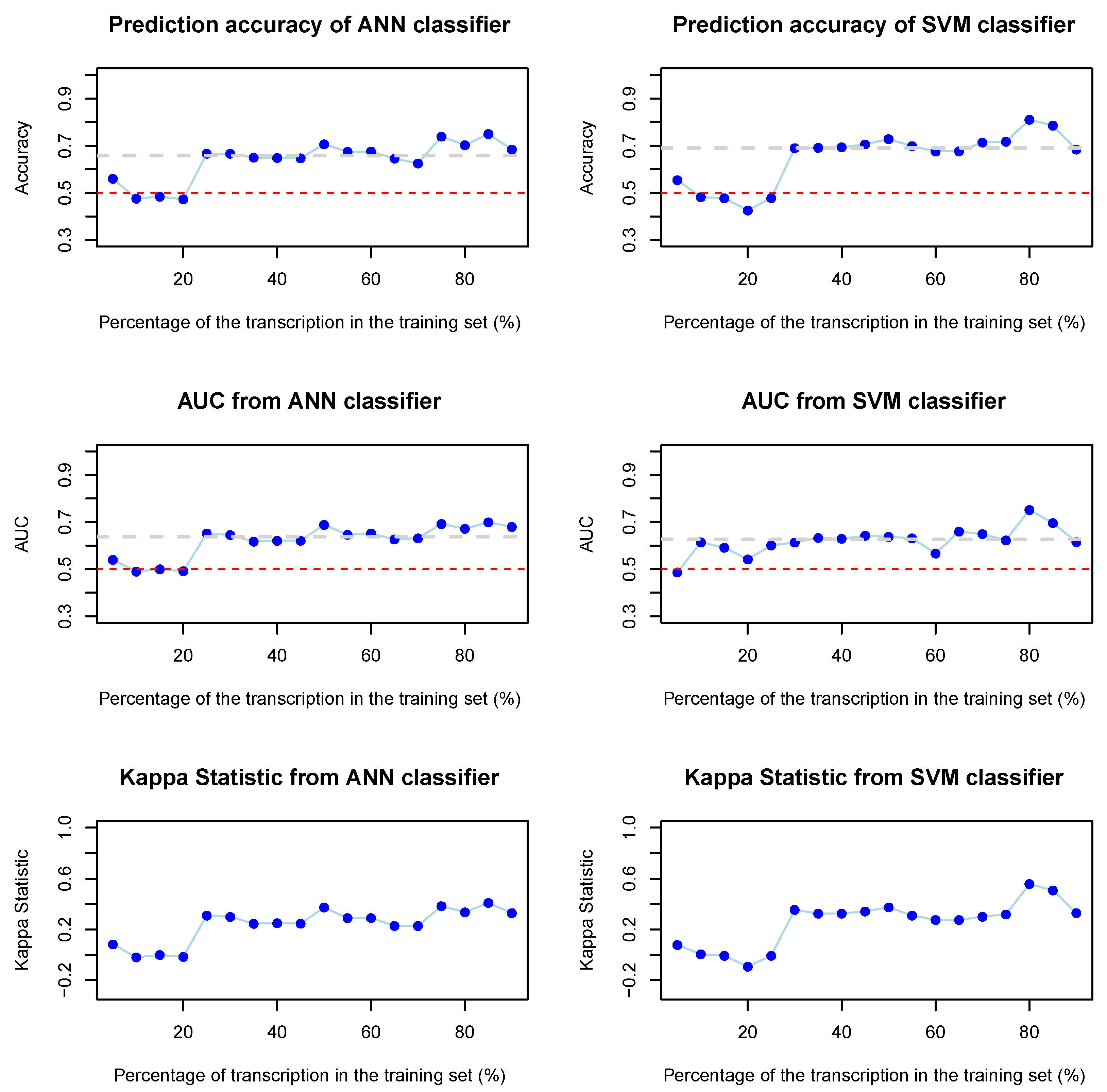
The results in Table 5 and Table 6 are also displayed in Figure 2 and Figure 3, respectively, for better visualisation and comparison. The left column plots of Figure 2 account for the LASSO classifier results, while the right ones for the decision tree. Analogously, the plots in the left column of Figure 3 refer to the results of the ANN, while the right column represents the results of the SVM. For each of these classifiers, we plot the evolution of the prediction accuracy (first row), the area under the curve (second row), and the kappa statistic (third row) as the percentage of the dataset in the training set (ordinate axis) increases. The red dashed lines in the plots symbolise the worst-case scenario in which the classifier has no predictive value, i.e., an accuracy of 50% and an AUC of 0.5. Moreover, the light grey dashed line represents the obtained median values of the displayed metric. The latter coloured lines are not shown in the graphs of the kappa statistic because this metric is much more subjective than the other two in the sense that there is no exact point representing the case where the classifier has no predictive value. Furthermore, this metric is only useful for tracking possible random assignments for a given case, which results in its median not being very informative.

The LASSO classifier provides a median accuracy of 80.7% and a median AUC of 0.85. Despite some isolated downshifts, we observe a general improvement in the latter performance metrics as the amount of training samples increases. When we take a look at the plot of the kappa statistic of the LASSO classifier (first column, last row plot), we notice that the downshifts in the previous metrics are accompanied by a decrease in the kappa statistic. Thus, in these particular cases, the probability of a random match is higher, leading to a worsening of the predictions.

It is also worth noting that these drops in the performance metrics occur more frequently as the percentage of training samples increases. In some way, this makes sense, because, as the cardinality of the training set increases, the cardinality of the test set decreases while containing a high percentage of short text fragments. This increases the probability of the random assignment of test samples, because, occasionally, none of their words appear in the set of unique words of the training set.

To exemplify the above reasoning, if the training set is 70% of the original dataset, as reported in the second column of Table 4, we have that $\mathcal{T}=\{F_1,\dots ,F_{128}\}$ and $\mathcal{E}=\{F_{129},\dots ,F_{184}\}$. Thus, there are 56 text fragments in the test set and 23 that consist of less than 5 words (see the fifth column of Table 4). Among the 23, $F_{179},F_{181}\in {\mathfrak{S}}^1$ are two text fragments in the test set whose words are not in the set of unique words within the training set. Thus, they are classified at random because their representation is the null vector. However, when considering 80% of the dataset as the training set, the text fragment $F_{179}\in {\mathfrak{S}}^1,$ although still in the test set, does have words in the set of unique words within the training set. Thus, no random classification occurs.

In the case of LASSO, it is noteworthy that for training sets consisting of more than 55% of the original dataset, the accuracy and AUC values computed in the test samples at issue are higher than the median values. The same is true for the SVM classifier applied to training sets with more than 50% of all text fragments. According to the conventions proposed in Section 4.3, the classification is excellent in terms of the AUC and substantial with regard to the kappa statistic.

On the other hand, the median prediction accuracy of the decision tree algorithm is 71.2% and the median AUC is 0.67. Just as in the case of the LASSO classifier, we observed some downshifts in the performance metrics, which are more pronounced this time. Once again, this behaviour can be explained by the evolution of the values of the kappa statistic.

Regarding the performance of the ANN, it is worth mentioning that it provides a median prediction accuracy of 70% and a median AUC of 0.67. These results are very similar to those of the decision tree, with the main difference being that the downshifts are now smoother. There is also a clearer tendency for the ANN to improve over the decision trees as the training set increases. However, the ANN cannot outperform LASSO, even when the training set is large. In addition, it was verified that ANNs are more time consuming than the other methods studied in this manuscript, since a huge number of parameters need to be adjusted.

As for SVM, it is a method that generally performs well. In particular, the median accuracy is 77% and the median AUC is 0.82, which means that SVM significantly outperforms both the decision tree and the ANN. Even more remarkable is the stability of the method, as evidenced by the absence of downward trends in the metrics examined, particularly in the kappa statistic. In fact, both the prediction accuracy and the AUC values for the SVM monotonically increase when the percentage of text fragments used as the training set increases.

Having said that, the performance of the LASSO classifier is better than that of the decision tree and ANN classifiers (in agreement with the performance metrics analysed in this manuscript). In order to find a reason for this fact, we resorted to the mathematical foundations of these classification methods. The main advantage of the LASSO classifier, which is not implemented in the decision tree algorithm nor in the ANN, is feature selection. As reported in the second column of Table 5 and Table 6, the dimension of the features used to feed our classification models ranges from 155 to 957, depending on the percentage chosen as the training set. This means that we are working with high-dimensional spaces, up to dimension 957. While the LASSO method alone is able to select the features that are more discriminative for the analysis by shrinking to zero some beta coefficients in Equation (2) of Section 4, this is not the case for the decision tree algorithm or ANN. This results in the tree not growing properly when it is decided to split upon certain features that may not be too relevant in the corpus or whose discriminative power is not as strong. Something similar happens with the ANN, where these non-informative variables contribute to making decisions based on noise. Furthermore, the LASSO regularisation helps to generalise better to new observations [7], which may explain the better performance of LASSO over the decision tree algorithm or ANN when evaluating the test samples.

In summary, both LASSO and SVM perform quite well on this dataset, the performance of SVM being comparable to that of LASSO. In particular, LASSO is slightly better in the 55–65% range, while SVM is better in the 70–90% range.

5.2. Analysis with Filtering

It is well known that not all words in a certain corpus contain the same amount of information, nor do they have the same discriminative power. Thus, a possible solution to this excess of irrelevant features is to filter the set of words in the analysis by removing the so-called stop words. The concept of stop words, coined by Hans Peter Luhn in 1960 [37], refers to common words that carry little or no significant information [7]. These words—typically determiners, articles, prepositions, and/or conjunctions—are stored in what we call a stop list and are usually filtered out before any task of processing data coming from natural language. Keeping in mind that there is no a universal stop list, we used the list of Spanish stop words available in the tm (acronym for Text Mining) R package [38].

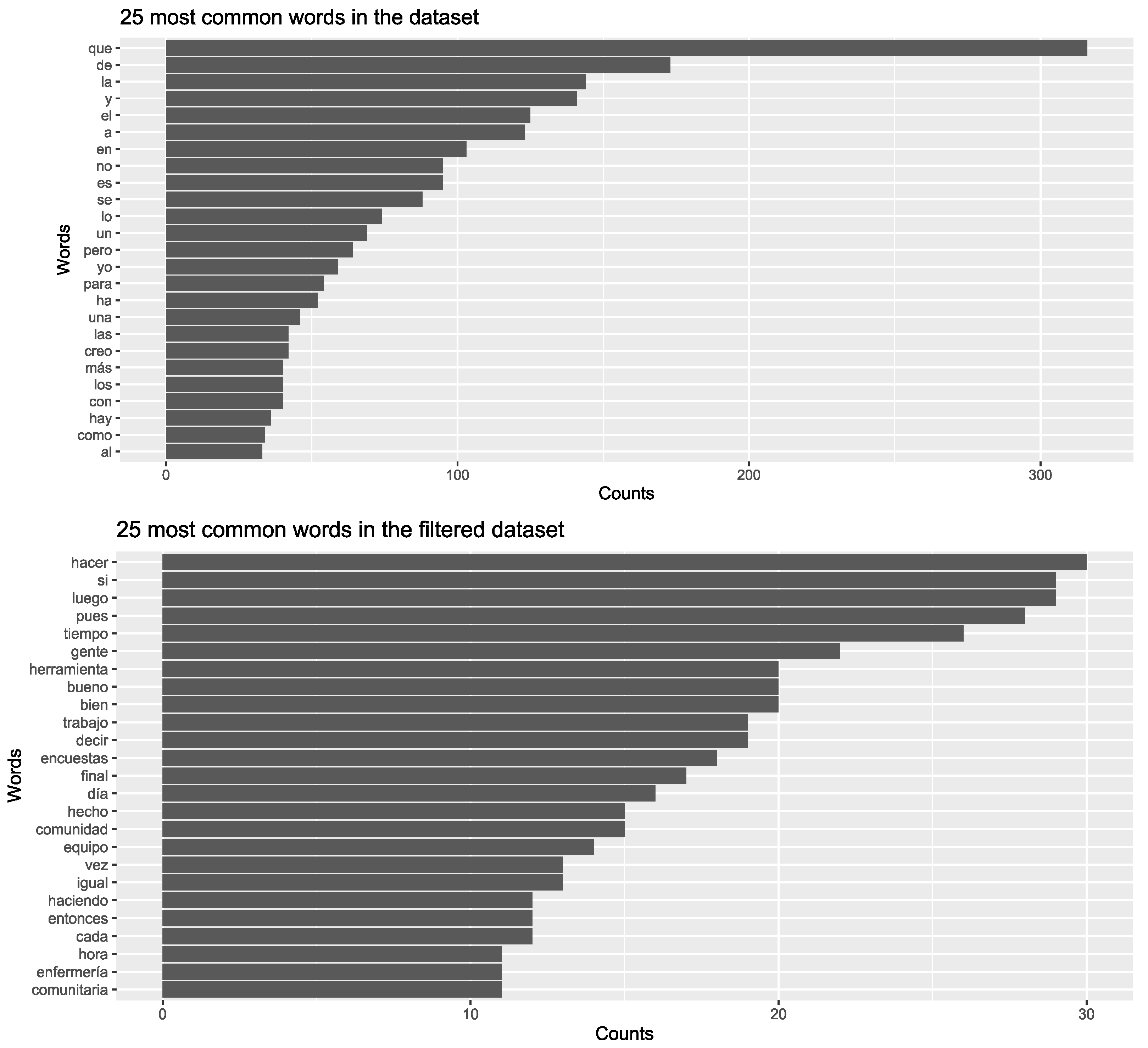
Removing the stop words from the original dataset drastically reduces the number of unique words used to compute our input features, i.e., the dimension of the vectors containing the tf–idf statistics. Our dataset originally contained 1024 unique words, but after filtering out the stop words, the number of unique words decreased to 883. Specifically, the stop words accounted for more than 10% of the original set of unique words.

In Figure 4, we plot the 25 most common words in our dataset before (top plot) and after (bottom plot) filtering out the stop words. Not only do we see that the raw counts (horizontal axis) of most frequent words decreases dramatically (from hundreds to dozens), but also that the frequency of the words that passed the filter is similar. While there were words in the original dataset that repeated significantly more frequently than others, the most frequent words in the filtered dataset occur more or less equally often in the corpus, i.e., they are quite balanced. As will be seen below, this filtering of the dataset will improve the performance of the C5.0 decision tree algorithm by avoiding splitting because of words that contain little information and/or are irrelevant in the corpus.

In addition to removing stop words, further limiting the number of words in the analysis would be an added bonus for the decision tree methodology. Indeed, restricting the number of words before calculating the tf–idf statistics would result in a much simpler model by not creating too many variables (dimension reduction) that sometimes contain irrelevant information.

It should be noted, however, that filtering the dataset is a double-edged sword, especially in a problem where the categories are defined by context. Indeed, it may happen that reducing the number of unique words helps to build a less complex method, but the price is the loss of information. Sometimes, this loss of information leads to a degradation in the performance of some classifiers. We will see below that this is precisely what happens for the LASSO, ANN, and SVM classifiers applied to the dataset under study.

Next, we performed another analysis, keeping only the 100 most-frequent words of the dataset after filtering out the stop words. The results are listed in

Table 7. Results of applying the two classification models, namely the LASSO (columns three to five) and the decision tree (columns six to eight), to the filtered dataset. The evolution of the accuracy (third and sixth columns), area under the ROC curve (fourth and seventh columns), and kappa (fifth and eighth columns) evaluation metrics as the percentage of the original dataset used as the training set (first column) increases is reported. Moreover, the number of unique words defining the dimension of the input vectors (second column) is 100 for each selected percentage.

Percentage	Unique	LASSO			C5.0 Decision Tree
	Words	Accuracy	AUC	Kappa	Accuracy	AUC	Kappa
5%	100	0.53	0.50	0.00	0.37	0.39	−0.21
10%	100	0.46	0.50	0.00	0.61	0.58	0.16
15%	100	0.62	0.62	0.19	0.64	0.63	0.25
20%	100	0.63	0.67	0.22	0.63	0.61	0.22
25%	100	0.62	0.60	0.19	0.62	0.60	0.19
30%	100	0.67	0.68	0.31	0.70	0.67	0.35
35%	100	0.74	0.74	0.43	0.65	0.60	0.21
40%	100	0.71	0.75	0.37	0.65	0.59	0.20
45%	100	0.73	0.72	0.39	0.74	0.68	0.40
50%	100	0.75	0.70	0.44	0.75	0.66	0.42
55%	100	0.76	0.69	0.45	0.72	0.65	0.33
60%	100	0.80	0.72	0.53	0.76	0.70	0.42
65%	100	0.75	0.75	0.42	0.74	0.63	0.36
70%	100	0.82	0.83	0.59	0.73	0.79	0.43
75%	100	0.85	0.81	0.63	0.87	0.85	0.69
80%	100	0.84	0.82	0.61	0.86	0.82	0.67
85%	100	0.82	0.83	0.58	0.86	0.85	0.67
90%	100	0.79	0.74	0.51	0.89	0.90	0.76

and

Table 8. Results of applying the artificial neural network (columns three through five) and support vector machine (columns six through eight) classification models, to the filtered dataset. The evolution of the accuracy (third and sixth columns), area under the ROC curve (fourth and seventh columns), and kappa (fifth and eighth columns) evaluation metrics as the percentage of the original dataset used as the training set (first column) increases is reported. Moreover, the number of unique words defining the dimension of the input vectors (second column) is 100 for each selected percentage.

Percentage	Unique	Artificial Neural Network			Support Vector Machine
	Words	Accuracy	AUC	Kappa	Accuracy	AUC	Kappa
5%	100	0.56	0.54	0.08	0.55	0.49	0.08
10%	100	0.48	0.49	−0.02	0.48	0.61	0.01
15%	100	0.48	0.50	0.00	0.48	0.59	−0.01
20%	100	0.47	0.49	−0.02	0.43	0.54	−0.09
25%	100	0.67	0.65	0.31	0.48	0.60	−0.01
30%	100	0.67	0.65	0.30	0.69	0.61	0.36
35%	100	0.65	0.62	0.25	0.69	0.63	0.33
40%	100	0.65	0.62	0.25	0.69	0.63	0.33
45%	100	0.65	0.62	0.25	0.71	0.64	0.34
50%	100	0.71	0.69	0.37	0.73	0.64	0.38
55%	100	0.67	0.65	0.29	0.70	0.63	0.31
60%	100	0.68	0.65	0.29	0.68	0.57	0.28
65%	100	0.65	0.63	0.23	0.68	0.66	0.28
70%	100	0.63	0.63	0.23	0.71	0.65	0.30
75%	100	0.74	0.69	0.38	0.72	0.62	0.32
80%	100	0.70	0.67	0.34	0.81	0.75	0.56
85%	100	0.75	0.70	0.41	0.79	0.70	0.51
90%	100	0.68	0.68	0.33	0.68	0.62	0.33

, which are similar in structure to Table 5 and Table 6, respectively. Note that the performance metrics generally improve as the size of the training set increases, except for some isolated downshifts due to the same reasons explained for the unfiltered case. These results are illustrated in Figure 5 and Figure 6, which again have the same format as Figure 2 and Figure 3.

In comparison to the non-filtered case, less sharp downshifts are seen in the plots of Figure 5 and Figure 6, with the exception of the SVM classifier. However, it is worth noticing no superior behaviour in the median within the analysed performance metrics, neither for LASSO, nor for the decision tree, ANN, or SVM. On the one hand, LASSO yields a median accuracy of 74.6% and a median AUC of 0.72, whereas the decision tree produces a median accuracy of 72.8% (just slightly higher than the unfiltered case) and a median AUC of 0.66. On the other hand, the median values of accuracy and AUC for ANN are 66% and 0.64, respectively, while the SVM classifier yields a median accuracy of 69% and a median AUC of 0.63. This clearly indicates that ANNs and SVMs perform significantly worse when filtering the dataset. Despite this, from Figure 5, we see that the performance of the decision tree classifier has clearly improved, as expected, for high percentages with respect to that of Figure 2. In light of the above, the LASSO and decision tree classifiers can be considered as roughly acceptable with respect to the AUC and moderate in terms of the kappa statistic in the filtered case, whereas the ANN and SVM are poor with regard to AUC and fair in terms of the kappa statistic (see Section 4.3). When the filtered and unfiltered cases are compared at each percentage, we observe that the prediction accuracy and the AUC for the LASSO, ANN, and SVM are slightly higher before filtering out the stop words. One explanation for this is that we actually lose information when we reduce the number of features in our analysis. Indeed, we took out some words from our original dataset that we assumed are generally irrelevant, but might be important in context, especially in an analysis such as that conducted in this manuscript, where the categories are abstractions of what is being said. Since the LASSO classifier itself is capable of performing feature selection—and therefore, can manage larger datasets with less risk than decision trees, ANNs and SVMs—this manual filtering does not make the difference. In fact, it follows from the data available that the results are marginally worse.

We also performed the analysis by filtering out only the stop words, without limiting the number of unique words in the model to the 100 most-frequent words in the dataset. The results are not reported here because they do not represent a large improvement and are somewhat worse for the LASSO and SVM as random assignments slightly increase. We attributed this to the fact that, when ordering the words from most frequent to less, the words from 101 to the less-frequent ones are uncommon in the corpus. In fact, their absolute frequency in the entire corpus is less than five counts, so their tf–idf statistics are small (close to zero). Thus, the fact that these words increase the dimensionality of the problem while having low discriminative power results in an increase of the probability of random classification.

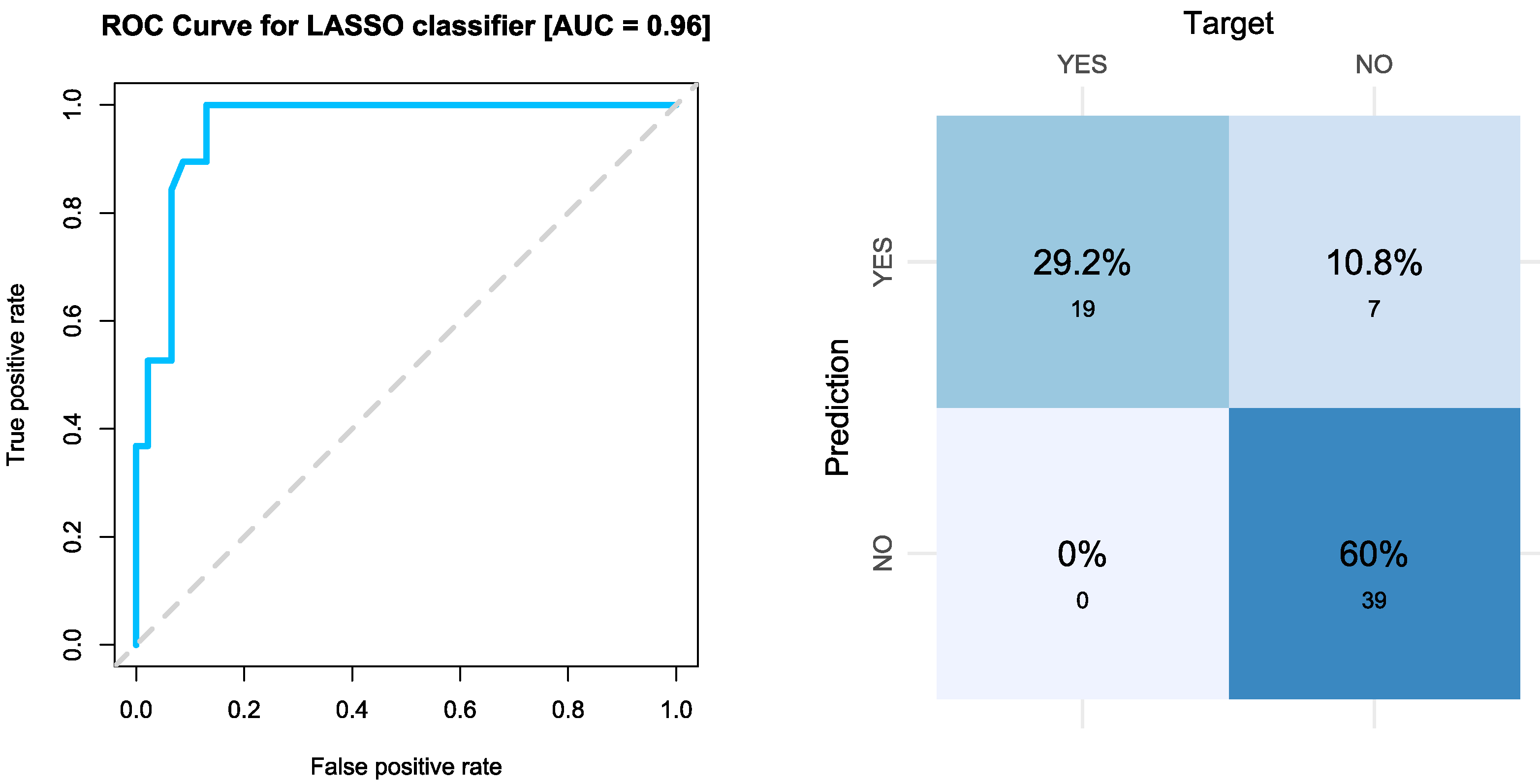
Even though the performance of the decision tree algorithm improved after filtering the dataset, the LASSO classifier without filtering appears to be the most appropriate method to deal with our initial binary classification problem. Indeed, the results obtained with LASSO are remarkably good and outperform even those obtained with the ANN and SVM, since after analysing and hand labelling only 65% of the unfiltered dataset, we can predict the labels of the 35% remaining text fragments with over 88% accuracy. The goodness of this classification is justified with an AUC of 0.96 (outstanding discrimination between classes) and a value for the kappa statistic of 0.77 (substantial strength of the agreement), as indicated in Table 5.

Finally, as an example, Figure 7 shows the ROC curve (left plot) and the confusion matrix (right plot) when evaluating the test samples $F_{120},\dots ,F_{184}$ in the model trained using the LASSO method and 65% of the original dataset. We can observe that there are no false negatives. This is particularly good in practice as the fragments that should be classified by the coders are all in the set of fragments predicted as containing a CFIR construct.

It is worth noting that LASSO was chosen because it is the method that provides the better performance with a lower percentage of participant transcription used as the training set. The reason is that our main goal is to find out to what extent it is necessary to manually code the text fragments in order to predict the remaining ones in an acceptable way. If we were looking for better prediction in classification, regardless of the amount of transcript to be read, the SVM would be the best candidate since its performance is higher in the 70–90% range of transcription used in the training set.

The proposed methodology has some limitations that we aim to tackle in future work. In particular, (i) to obtain the text fragments in Section 3, we made use of the pieces labelled by the trained coders. (ii) That the procedure allows saving time is only true if the fragments can be coded with validity outside of the contextual text that is being ignored. We justify them in that this work is a first venture into analysing this type of dataset from a statistical point of view. It is our understanding that these limitations can be solved by making use of whole paragraphs and not only of fragments of them. However, this would require having a larger amount of paragraphs, which in turn would allow extending this analysis to multi-classification methods to predict whether a text fragment belongs to one of the five possible domains proposed in the CFIR framework, rather than limiting ourselves to merely detecting the presence of any CFIR construct. Furthermore, it is worth noticing that the performed supervised classifications can be considered as problems in the high-dimensional misspecified binary classification framework, as the required assumptions have not been checked. This is a framework studied in [39] for the particular case of logistic regression.

6. Conclusions

This manuscript presents a novel study on the application of supervised classification to text data for CFIR construct coding. Our study revolves around a binary classification problem, which involves predicting whether or not a text fragment is assigned a CFIR construct. In particular, our dataset consisted a text file containing the transcription in Spanish of a focus group of the PVS Programme and another document in which CFIR constructs were assigned to specific parts of the transcription by a pair of trained coders. Regarding the applied utility of the method, the technique presented in this manuscript outputs a class label for each text fragment in the test sample: “1” if the considered text fragment potentially contains a CFIR construct, or “0” if not. In this way, qualitative researchers can automatically identify the parts of speech that might contain a CFIR construct. This may permit the coder to progress more rapidly through the manual coding because he/she is alerted to the more important text in the transcript.

Our approach to the binary classification problem is based on the application of four supervised classification models, namely the logistic LASSO regularisation, the C5.0 decision tree algorithm, artificial neural networks, and support vector machines. These models are applied after the raw dataset has been organised according to a novel procedure and then preprocessed, as is common in the literature; steps that were necessary to obtain numerical features from the raw text data. Manual feature selection via the removal of stop words was also performed aiming to ameliorate the results of the latter models. Even though the results of the decision tree improved after filtering out the stop words from the dataset, they could not outperform the results of LASSO in the unfiltered case. Moreover, it was shown that neural networks perform worse than LASSO and even the decision tree when the dataset is filtered, while SVM gives comparable results to LASSO on the original dataset. However, LASSO was shown to perform slightly better when the percentage of transcript fragments used as the training set is lower. This, together with the ability of LASSO to perform feature selection and regularisation simultaneously, led us to highly recommend this method for this type of classification problem.

In particular, the analysis performed on the dataset under discussion shows promising results, as making use of just 65% of the participant transcription as the training set, we obtained over an 88% success rate in predicting the assignment of text with CFIR constructs to be manually coded by the trained coder to the remaining 35%. There were only seven misclassifications of predicted CFIR text to manually coded CFIR text, and in all cases, these classifications were false positives. Thus, in the worst case, more text fragments have to be labelled by the trained coder, but none of the fragments containing a CFIR construct will be identified as less important. Even though the exact CFIR domain and construct still need to be identified by hand, the amount of handwork is potentially reduced.

The results of this initial study are promising and suggest that statistical and ML approaches may be beneficial to assist qualitative researchers in their analysis of the transcribed text collected in their research studies, especially when a structured framework such as the CFIR is used to guide data collection and analysis. Additional studies are warranted to explore and quantify the value added by this approach.

References

1. Pope, C.; Mays, N. Qualitative Research in Health Care, 3rd ed.; Blackwell Publishing: Hoboken, NJ, USA, 2006; Available online: https://onlinelibrary.wiley.com/doi/book/10.1002/9780470750841 (accessed on 7 April 2022).
2. Gale, R.C.; Wu, J.; Erhardt, T. Comparison of rapid vs in-depth qualitative analytic methods from a process evaluation of academic detailing in the Veterans Health Administration. Implement. Sci. 2019, 14, 11. [Google Scholar] [CrossRef] [PubMed] [Green Version]
3. Palinkas, L.A.; Mendon, S.J.; Hamilton, A.B. Innovations in mixed methods evaluations. Annu. Rev. Public Health. 2019, 40, 423–442. [Google Scholar] [CrossRef] [PubMed] [Green Version]
4. Vindrola-Padros, C.; Johnson, G.A. Rapid techniques in qualitative research: A critical review of the literature. Qual. Health Res. 2020, 30, 1596–1604. [Google Scholar] [CrossRef] [PubMed]
5. Grove, S.K.; Burns, N.; Gray, J. The Practice of Nursing Research: Appraisal Synthesis and Generation of Evidence, 9th ed.; Elsevier: St. Louis, MI, USA; Saunders: St. Louis, MI, USA, 2013; Available online: https://www.elsevier.com/books/burns-and-grove%27s-the-practice-of-nursing-research/978-0-323-67317-4 (accessed on 7 April 2022).
6. Le Glaz, A.; Haralambous, Y.; Kim-Dufor, D.H. Machine Learning and Natural Language Processing in Mental Health: Systematic Review. J. Med. Internet Res. 2021, 23, e15708. [Google Scholar] [CrossRef]
7. Hvitfeldt, E.; Silge, J. Supervised Machine Learning for Text Analysis in R, 1st ed.; CRC Press: New York, NY, USA, 2021. [Google Scholar] [CrossRef]
8. Rish, I. An Empirical Study of the Naïve Bayes Classifier. In Proceedings of the International Joint Conference on Artificial Intelligence: Workshop on Empirical Methods in Artificial Intelligence, Seattle, WA, USA, 4–10 August 2001; pp. 41–46. [Google Scholar]
9. Kuhn, M.; Johnson, K. Applied Predictive Modeling, 1st ed.; Springer: New York, NY, USA, 2013. [Google Scholar] [CrossRef]
10. Hastie, T.; Tibshirani, R. Statistical Learning with Sparsity, 1st ed.; CRC Press: New York, NY, USA, 2015. [Google Scholar] [CrossRef]
11. Boser, B.; Guyon, I.; Vapnik, V. A training algorithm for optimal margin classifiers. In Proceedings of the Fifth Annual Workshop on Computational Learning Theory, Pittsburgh, PA, USA, 27–29 July 1992. [Google Scholar]
12. Cristianini, N.; Shawe-Taylor, J. An Introduction to Support Vector Machines and Other Kernel-Based Learning Methods; Cambridge University Press: Cambridge, UK, 2000; Available online: www.support-vector.net (accessed on 20 May 2022).
13. Kim, S.M.; Han, H.; Park, J.M.; Choi, Y.J.; Yoon, H.S.; Sohn, J.H.; Baek, M.H.; Kim, Y.N.; Chae, Y.M.; June, J.J.; et al. A Comparison of Logistic Regression Analysis and an Artificial Neural Network Using the BI-RADS Lexicon for Ultrasonography in Conjunction with Introbserver Variability. J. Digit. Imaging 2012, 25, 599–606. [Google Scholar] [CrossRef]
14. Elman, J.L. Finding structure in time. Cogn. Sci. 1990, 14, 179–211. [Google Scholar] [CrossRef]
15. Collobert, R.; Weston, J.; Bottou, L.; Karlen, M.; Kavukcuoglu, K.; Kuksa, P. Natural language processing (almost) from scratch. J. Mach. Learn. Res. 2011, 12, 2493–2537. [Google Scholar]
16. Kalchbrenner, N.; Blunsom, P. Recurrent convolutional neural networks for discourse compositionality. In Proceedings of the Workshop on Continuous Vector Space Models and their Compositionality, Sofia, Bulgaria, 9 August 2013; pp. 119–126. [Google Scholar]
17. Fan, H.; Du, W.; Dahou, A.; Ewees, A.A.; Yousri, D.; Elaziz, M.A.; Elsheikh, A.H.; Abualigah, L.; Al-qaness, M.A.A. Social Media Toxicity Classification Using Deep Learning: Real-World Application UK Brexit. Electronics 2021, 10, 1332. [Google Scholar] [CrossRef]
18. Aldjanabi, W.; Dahou, A.; Al-qaness, M.A.A.; Elaziz, M.A.; Helmi, A.M.; Damaševičius, R. Arabic Offensive and Hate Speech Detection Using a Cross-Corpora Multi-Task Learning Model. Informatics 2021, 8, 69. [Google Scholar] [CrossRef]
19. Haynes, C.; Palomino, M.A.; Stuart, L.; Viira, D.; Hannon, F.; Crossingham, G.; Tantam, K. Automatic Classification of National Health Service Feedback. Mathematics 2022, 10, 983. [Google Scholar] [CrossRef]
20. Lee, E.; Lee, C.; Ahn, S. Comparative Study of Multiclass Text Classification in Research Proposals Using Pretrained Language Models. Appl. Sci. 2022, 12, 4522. [Google Scholar] [CrossRef]
21. Damschroder, L.J.; Aron, D.C. Fostering implementation of health services research findings into practice: A consolidated framework for advancing implementation science. Implement. Sci. 2009, 4, 50. [Google Scholar] [CrossRef] [PubMed] [Green Version]
22. Rogers, H.L.; Pablo-Hernando, S.; Núñez-Fernández, S. Barriers and facilitators in the implementation of an evidence-based health promotion intervention in a primary care setting: A qualitative study. J. Health Organ. Manag. 2021, 35, 349–367. [Google Scholar] [CrossRef] [PubMed]
23. Manning, C.D.; Raghavan, P. Introduction to Information Retrieval, 1st ed.; Cambridge University Press: New York, NY, USA, 2008. [Google Scholar] [CrossRef]
24. Intarapaiboon, P. A Framework for Text Classification Using Intuitionistic Fuzzy Sets; Springer: Berlin/Heidelberg, Germany, 2019; pp. 737–746. [Google Scholar] [CrossRef]
25. Sidiropoulos, G.K.; Diamianos, N.; Apostolidis, K.D.; Papakostas, G.A. Text Classification Using Intuitionistic Fuzzy Set Measures—An Evaluation Study. Information 2022, 13, 235. [Google Scholar] [CrossRef]
26. Tibshirani, R. Regression Shrinkage and Selection via the Lasso. J. R. Stat. Soc. Ser. B 1996, 58, 267–288. Available online: http://www.jstor.org/stable/2346178 (accessed on 11 March 2022). [CrossRef]
27. Vasquez, M.M.; Hu, C. Least absolute shrinkage and selection operator type methods for the identification of serum biomarkers of overweight and obesity: Simulation and application. BMC Med. Res. Methodol. 2016, 16, 154. [Google Scholar] [CrossRef] [Green Version]
28. Lantz, B. Machine Learning with R: Expert Techniques for Predictive Modeling, 3rd ed.; Packt Publishing: Birmingham, UK, 2019. [Google Scholar]
29. Fang, C.; Dong, H.; Zhang, T. Mathematical models of overparameterized neural networks. Proc. IEEE 2021, 109, 683–703. [Google Scholar] [CrossRef]
30. Kingma, D.P.; Ba, J. Adam: A method for stochastic optimization. arXiv 2014, arXiv:1412.6980. [Google Scholar]
31. Cortes, C.; Vapnik, V. Support-vector networks. Mach. Learn. 1995, 20, 273–297. [Google Scholar] [CrossRef]
32. Hastie, T.; Tibshirani, R.; Friedman, J.H. The Elements of Statistical Learning: Data Mining, Inference, and Prediction, 1st ed.; Springer: New York, NY, USA, 2001. [Google Scholar] [CrossRef]
33. Cohen, J. A Coefficient of Agreement for Nominal Scales. Educ. Psychol. Meas. 1960, 20, 37–46. [Google Scholar] [CrossRef]
34. Laandis, J.R.; Koch, G.G. The Measurement of Observer Agreement for Categorical Data. Biometrics 1977, 33, 159–174. [Google Scholar] [CrossRef] [Green Version]
35. Hosmer, D.W.; Lemeshow, S. Applied Logistic Regression, 2nd ed.; Wiley: New York, NY, USA, 2000; pp. 160–162. [Google Scholar] [CrossRef]
36. Wickham, H.; Averick, M. Welcome to the tidyverse. J. Open Source Softw. 2019, 4, 1686. [Google Scholar] [CrossRef]
37. LuhnKey, H.P. Key word-in-context index for technical literature (kwic index). J. Assoc. Inf. Sci. Technol. 1960, 11, 288–295. [Google Scholar] [CrossRef] [Green Version]
38. Feinerer, I.; Hornik, K. Text Mining Infrastructure in R. J. Stat. Softw. 2008, 25, 1–54. [Google Scholar] [CrossRef] [Green Version]
39. Furmańczyk, K.; Rejchel, W. Prediction and Variable Selection in High-Dimensional Misspecified Binary Classification. Entropy 2020, 22, 543. [Google Scholar] [CrossRef]
Figure 1. The total entropy H as a function of the proportion p of text fragments in class “1”.
Mathematics 10 02005 g001
Figure 2. Graphical representation of the evolution of the performance metrics for the LASSO (left column) and decision tree (right column) classifiers as the percentage of the original dataset used as the training set (ordinate axis) increases. For each method, we plot the precision accuracy (first row), the area under the ROC curve (second row), and the kappa statistic (third row). The red dashed line represents the situation where the classifier has no predictive power, and the grey dashed line represents the median value for the different performance metrics.
Mathematics 10 02005 g002
Figure 3. Graphical representation of the evolution of the performance metrics for the artificial neural network (left column) and support vector machine (right column) classifiers as the percentage of the original dataset used as the training set (ordinate axis) increases. For each method, we plot the precision accuracy (first row), the area under the ROC curve (second row), and the kappa statistic (third row). The red dashed line represents the situation where the classifier has no predictive power, and the grey dashed line represents the median value for the different performance metrics.
Mathematics 10 02005 g003
Figure 4. The 25 most common words in the studied dataset before (top plot) and after (bottom plot) filtering out the stop words from the tm package. We notice that the stop words (such as “que”, “de”, “la”, “y”, “el”, “en”, etc.) disappeared after the filtering. Moreover, it is worth noting that the frequency (horizontal axis) of the removed stop words is much higher than the frequency of words of interest.
Mathematics 10 02005 g004
Figure 5. Graphical representation of the evolution of the performance metrics for the LASSO (left column) and decision tree (right column) classifiers as the percentage of the filtered dataset used as the training set (ordinate axis) increases. For each method, we plot the precision accuracy (first row), the area under the ROC curve (second row), and the kappa statistic (third row). The red dashed line represents the situation where the classifier has no predictive power, and the grey dashed line represents the median value for the different performance metrics.
Mathematics 10 02005 g005
Figure 6. Graphical representation of the evolution of the performance metrics for the artificial neural network (left column) and support vector machine (right column) classifiers as the percentage of the filtered dataset used as the training set (ordinate axis) increases. For each method, we plot the precision accuracy (first row), the area under the ROC curve (second row), and the kappa statistic (third row). The red dashed line represents the situation where the classifier has no predictive power, and the grey dashed line represents the median value for the different performance metrics.
Mathematics 10 02005 g006
Figure 7. ROC curve (left plot) and confusion matrix (right plot) resulting from evaluating the test samples F 120 , , F 184 in the model trained with the LASSO method using 65% of the original dataset, i.e., F 1 , , F 119 . The ROC curve plots the true positive rate (abscissa axis) versus the false positive rate (ordinate axis). The confusion matrix shows the proportion of true positives (top left corner), false positives (top right corner), the false negative (bottom left corner), and true negatives (bottom right corner).
Mathematics 10 02005 g007