Human Alertness Optimization with a Three-Process Dynamic Model

Abstract

Circadian rhythm is an important biological process for humans as it modulates a wide range of physiological processes, including body temperature, sleep-wake cycle, and cognitive performance. As the most powerful external stimulus of circadian rhythm, light has been studied as a zeitgeber to regulate the circadian phase and sleep. This paper addresses the human alertness optimization problem, by optimizing light exposure and sleep schedules to relieve fatigue and cognitive impairment, in cases of night-shift workers and subjects with certain mission periods based on dynamics of the circadian rhythm system. A three-process hybrid dynamic model is used for simulating the circadian rhythm and predicting subjective alertness and sleepiness. Based on interindividual difference in sleep type and living habits, we propose a tunable sleep schedule in the alertness optimization problem, which allows the appropriate tuning of sleep and wake times based on sleep propensity. Variational calculus is applied to evaluate the impacts of light and sleep schedules on the alertness and a gradient descent algorithm is proposed to determine the optimal solutions to maximize the alertness level in various cases. Numerical simulation results demonstrate that the cognitive performance during certain periods can be significantly improved by optimizing the light input and tuning sleep/wake times compared to empirical data.

1. Introduction

Circadian rhythm plays a significant role in our lives as it regulates various physiological processes, biological features, and behaviors. Circadian rhythm has evolved to oscillate with a period of about 24 h to keep in synchronization with the light-dark cycle on earth. Plasma melatonin suppression [1], circadian gene expression [2], and cognitive performance [3] demonstrate spectral sensitivity to light, i.e., they are more sensitive to short-wavelength light [4]. Numerous circadian rhythm models have been formulated and analyzed based on the dynamics of circadian-related physiological features [5]. Light has been widely used as an external input in circadian rhythm regulation in previous works [6]: Diekman constructed a one-dimensional map to demonstrate the process that the light-dark cycle entrains circadian rhythm dynamics [7]; Booth formulated a simplified dynamical system to investigate the dynamics in circadian regulation of sleep-wake cycle [8]; Abel and Doyle applied the model predictive control method on the dynamics of the mammalian circadian clock and showed theoretical results of circadian phase resetting via light [9]; Julius and Forger applied variational calculus on humans’ core body temperature dynamic model, and showed the optimized timing of light exposure dramatically reduced the circadian rhythm entrainment time in various time shifts [10,11]. Cognitive impairments, because of circadian disturbance, sleep disorder, and extended wakefulness, are common in modern society and bring negative impacts on our health. Lower concentration and alertness also cause harmful consequences, such as a decline in efficiency, traffic accident, and other failures in jobs and lives. In our common lives, we may give higher priority to the enhancement of our cognitive performance, alertness, and vigilance instead of reducing the time costs of entraining the misaligned circadian rhythm to a normal one. For example, transmeridian travelers who want to catch an important conference or have important personal matters at the destination, night-shift workers who need to relieve fatigue for a whole night, or soldiers with an important mission want to keep fresh. The light exposure should be appropriately set in terms of the dynamics of subjects’ cognitive functions to relieve cognitive impairments.

Previous research has shown that the dynamics of humans’ neurobehavior, cognitive performance, fatigue, and alertness are jointly determined or mutually affected by several processes, including circadian rhythm and sleep-wake cycle [12]. Empirical data showed that humans’ sleep-wake cycle is closely linked to the circadian rhythm and sleep homeostasis, called Process C and Process S, respectively [13]. Two-process models have been formulated to simulate the sleep-wake cycle and sleep propensity [14]. However, some experimental results indicated that the alertness level starts at a very low level at the wake-onset time and then increases rapidly. This phenomenon is attributed to sleep inertia, which is ignored in two-process models. To incorporate its impacts, the dynamics of the sleep inertia (usually called Process W) were formulated [15,16] and the three-process models, combining the two-process model with the sleep inertia, were used in several papers [17,18] to predict cognitive functions and alertness.

Several existing two-process and three-process models took the circadian process as predetermined skewed sinusoidal waveforms without consideration of light exposure. However, experimental studies indicated light intensity and spectrum during night-shift has a great influence on the alertness level of shift workers: the work in [19] showed exposure to bright light during nighttime slowed down the decline in alertness during the night-shift. Another study in [4] showed that subjective alertness at 8 am (the end of night-shift) was less impaired by staying in darkness or wearing circadian light-blocking goggles filtering light spectrum less than 480 mm than staying in unfiltered light exposure during the night-shift between 8 pm and 8 am. Achermann formulated a three-process model with Process C represented by a simpler core body temperature (CBT) model, which contains lighting impacts on its dynamics [16]. However, the CBT model had been developed several times to incorporate higher-order nonlinearities to capture the latest empirical data and experimental observation that amplitude recovery of circadian oscillator is slower around the singular regions than near the limit cycle [10], which has been ignored in the three-process model formulation. Previous literature optimized the sleep schedule to regulate cognitive performance [20]. However, this study ignored the constraints of sleep propensity [16] and deliberately changed the sleep and wake times. In addition, the existing study of light-based circadian entrainment [10,11] used light exposure to entrain Process C but ignored constraints of Process S and the sleep-wake cycle. Results of these studies also contain long wakefulness duration (or long duration under light exposure) beyond normal sleep times and excessive sleep propensity, which could be impractical for human subjects.

In this paper, we develop the three-process model and study the alertness optimization problem based on this model. The main contributions of this paper are as follows:

• This paper simulates the subjective alertness and sleepiness with various light inputs and sleep schedules by a three-process hybrid dynamic model. Different from previous work [14,16], the latest dynamic model of CBT [10,11] is used to represent the Process C in the three-process model to incorporate the lighting effects and higher-order nonlinear terms of circadian rhythm on cognitive performance;
• This paper proposes a tunable sleep schedule with appropriate sleep/wake time constraints in the three-process model to avoid excessive sleepiness and guarantee the optimal sleep schedule and light exposure are more practical for human subjects to follow;
• The numerical solution method of optimal light exposure and sleep schedule in alertness optimization problems is proposed based on the calculus of variations, and the results demonstrate that, compared with empirical data, the optimized light and sleep schedule relieve humans’ cognitive impairment caused by shift works and other issues.

In Section 2, the three-process hybrid dynamic model with light input is formulated and validated, and the problem formulations of several alertness optimization cases with light and sleep constraints are proposed. In Section 3, the numerical algorithm for solving the alertness optimization problems is proposed. In Section 4, the solutions of alertness optimization problems are demonstrated and compared with previous experimental data to discuss the regulation capability of light and sleep on human cognitive performance. Finally, the conclusion is summarized in Section 5.

2. Mathematic Model and Problem Formulation

We represent the Process C of the three-process model based on the CBT circadian rhythm dynamic model in [10,11]. The mathematical formulation of the CBT model is listed as follows:

$$\frac{dn}{dt}=60[{\alpha }_0·{\left(\frac{I}{I_0}\right)}^p·(1-\beta )·(1-n)-\gamma n],$$

(1)

$$u=G·{\alpha }_0·{\left(\frac{I}{I_0}\right)}^p·(1-\beta )·(1-n),$$

(2)

$$\frac{dx}{dt}=\frac{\pi }{12}\left[x_c+\mu \left(\frac{1}{3}x+\frac{4}{3}{x}^3-\frac{256}{105}{x}^7\right)+(1-0.4x)(1-k_c{x}_c)u\right],$$

(3)

$$\frac{d{x}_c}{dt}=\frac{\pi }{12}\left[q{x}_c(1-0.4x)(1-k_c{x}_c)u-{\left(\frac{24}{0.99729{\tau }_x}\right)}^{2}x-kx(1-0.4x)(1-k_c{x}_c)u\right],$$

(4)

where parameter values are given as ${\alpha }_0=0.05$ h⁻¹, $\gamma =0.0075$ h⁻¹, $I_0=9500$ lux, $p=0.5$, $G=33.75$, $\mu =0.13$ h⁻¹, $q=1/3$, ${\tau }_x=24.2$ h, $k=0.55$ h⁻¹, and $k_c=0.4$ h [10,11]. The term I represents the light input with a unit of $lux$. $\beta \in \{0,1\}$ represents the sleep state, i.e., $\beta \left(t\right)=1$ means the subject is sleeping at time t and $\beta \left(t\right)=0$ means the subject is awake. The state n in Equation (1) is the receptor state used to simulate the time-varying relation between the light input I and circadian drive u. The state x is the normalized state of CBT and $x_c$ is a complementary state.

The sleep homeostatic oscillator, i.e., Process S, represents the accumulation of substance that generates the sleep drive [16]. The dynamics of sleep homeostasis H are given as

$$\frac{dH}{dt}=\left\{\begin{array}{cc}-H/{\tau }_d,& \beta \left(t\right)=1,\\ (1-H)/{\tau }_r,& \beta \left(t\right)=0,\end{array}\right.$$

(5)

where the time constants during sleep and wake periods are ${\tau }_d=4.2$ h and ${\tau }_r=18.2$ h, respectively [16]. Sleep propensity $\Phi$ is jointly affected by both Process S and Process C. We define its value as

$$\Phi \left(t\right)=H\left(t\right)-A_{c}x\left(t\right).$$

(6)

where $A_c=0.1333$. If a subject falls asleep and wakes up spontaneously, the change in his sleep state $\beta \left(t\right)$ is fully determined by $\Phi \left(t\right)$ (and thus, essentially, by $H\left(t\right)$ and $x\left(t\right)$). The dynamic of the spontaneous sleep schedule is expressed as

$$\beta \left(t\right)=F_{\beta }(t,\beta \left(t^{-}\right))=\left\{\begin{array}{cc}1,& \Phi \left(t\right)=H_m,\\ 0,& \Phi \left(t\right)=L_m,\\ \beta \left(t^{-}\right),& \mathrm{otherwise},\end{array}\right.$$

(7)

where $t^{-}$ is the time just before t, i.e., $\beta \left(t^{-}\right)$ means the left limit of $\beta \left(t\right)$. The upper and lower bounds of spontaneous sleep schedule are $H_m=0.67$ and $L_m=0.17$, respectively [16]. The dynamic of sleep inertia W with sleep state is given as

$$\frac{dW}{dt}=-\frac{1-\beta }{{\tau }_W}W,$$

(8)

where the time constant ${\tau }_W=0.662$ h [16,20]. At the wake (onset) time, the value of sleep inertia W is reset to 0.32. The three-process model used in this paper consists Process C in Equations (1)–(4), Process S in Equation (5), and Process W in Equation (8). We define the value of alertness and sleepiness level, denoted as $A\left(t\right)$ and $B\left(t\right)$, as

$$A\left(t\right)=[1-\beta \left(t\right)][1+A_{c}x\left(t\right)-H\left(t\right)-W\left(t\right)].$$

(9)

$$B\left(t\right)=1-A\left(t\right).$$

(10)

The alertness level during sleep is set (by definition) as 0. Under a periodic light-dark cycle, the state of the three-process model, which is denoted as

$$\xi \left(t\right)={[n\left(t\right),x\left(t\right),x_c\left(t\right),H\left(t\right),W\left(t\right)]}^T\in {\mathbb{R}}^5,$$

may run periodically in the same period, i.e., the three-process model keeps synchronization with the light-dark cycle. We define a 24 h periodic light-dark cycle in the following form

$$I_{\mathrm{ref}}\left(t\right)=\left\{\begin{array}{cc}1000lux,& t\mathrm{mod}24\in [0,16),\\ 0,& t\mathrm{mod}24\in [16,24),\end{array}\right.$$

(11)

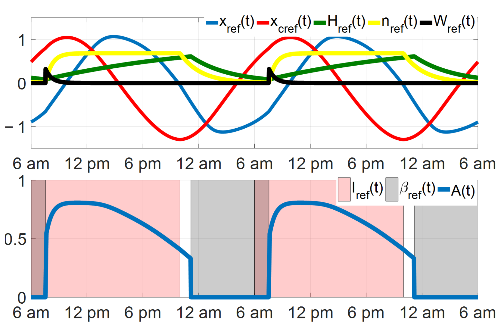
which simply simulates the reference daily light-dark cycle. We set that the sunrise/light-on time $t=0$ corresponds to 6 am and the sunset/light-off time $t=16$ corresponds to 10 pm. Under the periodic light-dark cycle in Equation (11) and the spontaneous sleep schedule in Equation (7), the state of the three-process model runs periodically in the same period. The stable periodic solution of the three-process model is the reference state ${\xi }_{\mathrm{ref}}\left(t\right)$, denoted as

$${\xi }_{\mathrm{ref}}\left(t\right)={[n_{\mathrm{ref}}\left(t\right),x_{\mathrm{ref}}\left(t\right),x_{c\mathrm{ref}}\left(t\right),H_{\mathrm{ref}}\left(t\right),W_{\mathrm{ref}}\left(t\right)]}^T,$$

which, along with the corresponding sleep state ${\beta }_{\mathrm{ref}}\left(t\right)$ and alertness level, is plotted in Figure 1. We can observe the daily alertness starts from a low level at the wake time, as a result of sleep inertia, then increases rapidly and reaches the daily maximum value at about 9 am. Then alertness declines steadily in the afternoon and evening until sleep begins, which agrees with daily profiles of cognitive performance and subjective sleepiness [21,22]. Note the post-lunch dip in alertness is widely experienced during the early afternoon in human beings, especially habitual nappers. Experimental observations of university students showed the alertness of these subjects show a progressive increase and peaks before noon, and slightly declines around noon to 4 pm. Then alertness increases again and reaches another peak, finally demonstrating a sharp drop to sleep [23]. One way to simulate the biphasic sleep pattern and post-lunch dips is by tuning the upper and lower thresholds in Equation (7) to generate one short and one long daily sleep bouts [14]. Another way for post-lunch dips’ simulation is adding another process (usually called Process U) with a period of 12 h [24]. Sleep and nap habits, as well as the extent of post-lunch dip, vary largely with persons and regions, here we study the alertness improvement problem with external light and sleep regulation, in which we assume the sleep is consolidated into one continuous nocturnal bout by long-term, daily 16-h photoperiod [22] and we only tune this single bout in the tunable sleep schedule. Experimental data of night-shift we compared in this paper comes from constant routine protocol and photoperiod experiments, which prohibited daytime naps and no obvious post-lunch dip was found in these experiments. Therefore, this model is sufficient for our simulation and study.

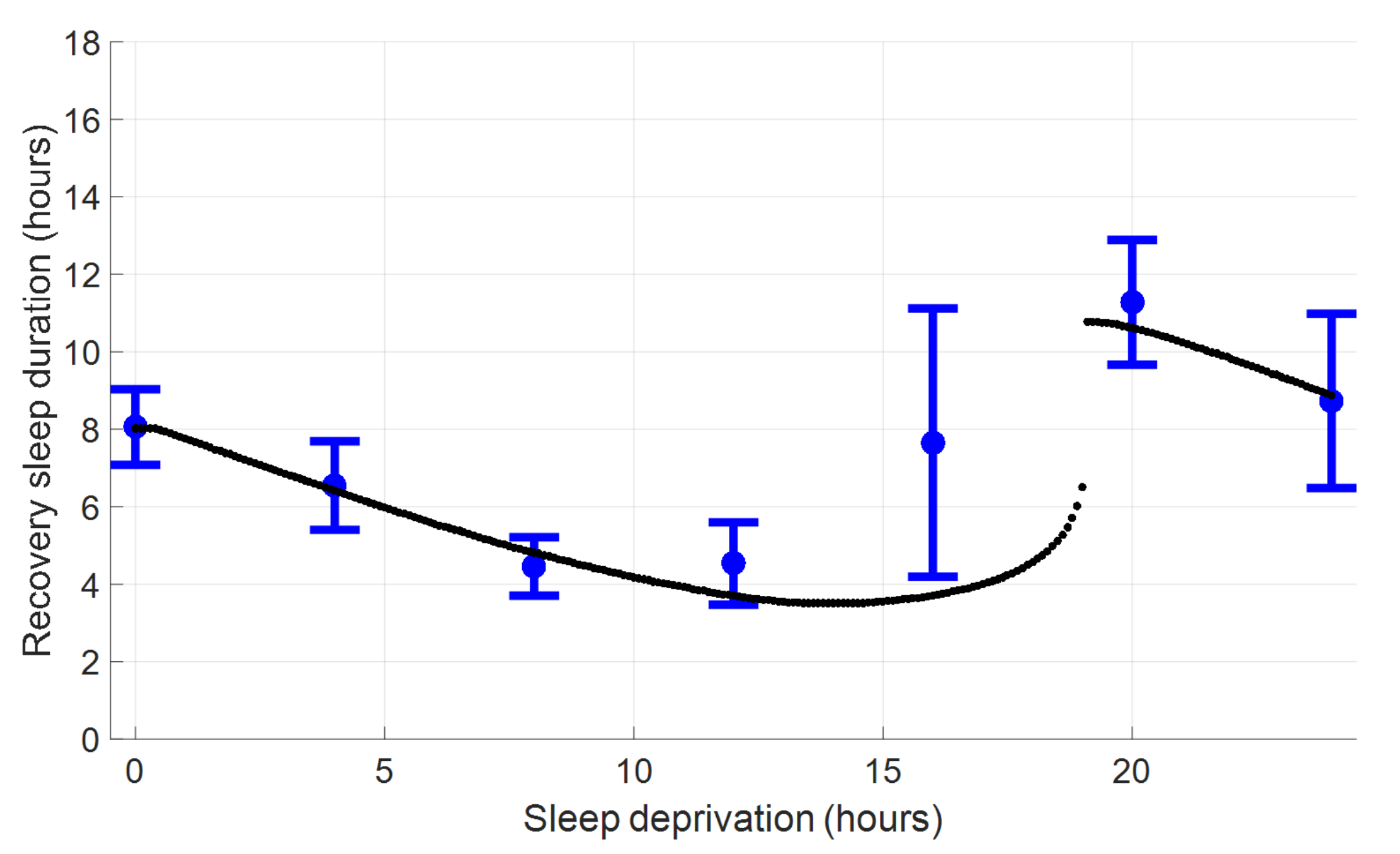
Sleep propensity and recovery sleep duration (after sleep deprivation) both do not monotonically increase with the time length of sleep deprivation (duration of keeping awake after spontaneous sleep time) [13], which can be simulated and explained by the three-process model. The simulation results of the three-process model and experimental data in [25] in Figure 2 both indicate the recovery sleep duration firstly shows a decline as the sleep deprivation increases from 0 to about 14 h, and then shows a discontinuous increase to a duration longer than normal night sleep when sleep deprivation is around 18 h. 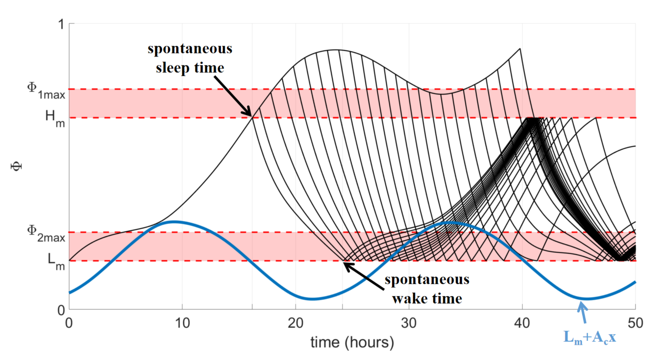Figure 3 shows the simulated sleep propensity during sleep deprivation with various time lengths and the following recovery sleep duration. After spontaneous sleep time, the sleep propensity firstly grows with the duration of sleep deprivation but then shows a decline when the sleep deprivation duration increases to more than 8 h, as a result of the increase in x from Process C reducing circadian sleep drive. This simulation is consistent with the fact that subjects may feel less fatigue and cannot fall asleep immediately once the night-shift work ends or having kept awake for several hours beyond normal sleep time. The blue curve of $L_m+A_{c}x$ in Figure 3 indicates the sleep homeostasis at wake time after sleep deprivation and determines the recovery sleep duration based on Equation (5). As the sleep deprivation duration increase to 14 h, the corresponding homeostasis at wake time increases gradually and shortens the recovery sleep duration after sleep deprivation. When the sleep deprivation duration increases from 14 to about 18 h, the homeostasis at the following wake time shows a sharp drop, resulting in a sudden growth in recovery sleep duration. Then, $L_m+A_c·x$ increases again and reduces the recovery sleep duration as the sleep deprivation continues to increase to more than 20 h.

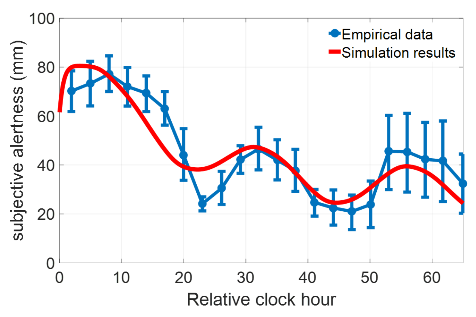
To further validate the accuracy of the three-process model in the prediction of subjective alertness and sleepiness, we introduce and simulate two experimental protocols in the previous reference. The first experiment asked subjects to remain awake for an extended period of 36–60 h under constant light (150 lux), which is called the constant routine experiment protocol [26]. Subjective alertness was assessed three times every hour using a linear 100-mm bipolar visual-analogue scale (VAS) during the experiment, which is a questionnaire that asks subjects to indicate their alertness on a visual scale of 100 mm length. We use the three-process model to simulate this experimental protocol and predict the subjective alertness, as shown in Figure 4. Note that the alertness value $A\left(t\right)$ in the three–process model has no unit. To fit the empirical units (0–100 mm), we scale the predicted subjective alertness as

$$\mathrm{subjective}\mathrm{alertness}\left(\mathrm{in}\mathrm{VAS}\right)=56.18\mathrm{mm}\times \frac{A\left(t\right)-0.26}{0.85}+45.07\mathrm{mm},$$

(12)

where 56.18 mm and 0.85 are the differences between maximum and minimum in empirical data and simulation results, 45.07 mm and 0.26 are the average values in empirical data and simulation results. The average mean square error between predicted alertness and the average empirical data is 7.91 mm, smaller than the standard deviation of the empirical data (9.80 mm). The coefficient of determination of the predicted alertness to the empirical data is 0.811. As shown in Figure 4, the predicted alertness from the three-process model shows good correspondence to the subjective alertness in empirical data.

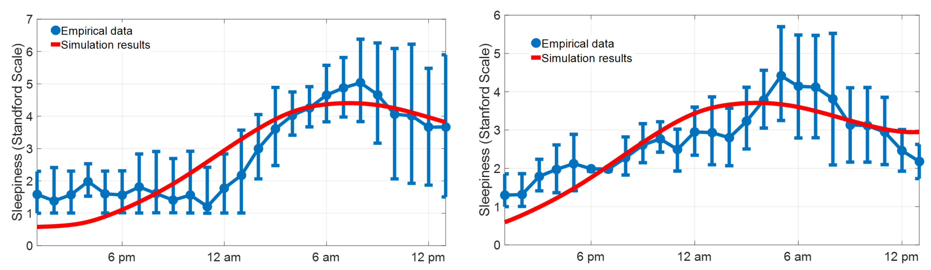
The second experiment, called photoperiod experiment in [22], asked subjects to stay in two different photoperiods: the long photoperiod has 16 h daily light in one week and the short has 10 h daily light in four weeks. The 24 h profiles of sleepiness were measured during a constant routine protocol with dim light less than 1 lux after each photoperiod by Stanford Sleepiness Scale ratings. To fit the Stanford Sleepiness Scale (SSS), the predicted sleepiness from the three-process model is scaled as

$$\mathrm{sleepiness}\left(\mathrm{in}\mathrm{SSS}\right)=3.83\times \frac{B\left(t\right)-0.62}{0.61}+2.83.$$

(13)

The corresponding values of alertness in VAS and sleepiness in SSS with respect to $A\left(t\right)$ and $B\left(t\right)$ in the three-process model are listed in

Table 1. The relationship of alertness in VAS (mm), $B\left(t\right)$, and sleepiness in SSS with $A\left(t\right)$.

$\mathit{A}\left(\mathit{t}\right)$	Alertness in VAS	$\mathit{B}\left(\mathit{t}\right)$	Sleepiness in SSS
0	27.89	1	5.22
0.1	34.49	0.9	4.59
0.2	41.10	0.8	3.96
0.3	47.71	0.7	3.33
0.4	54.32	0.6	2.70
0.5	60.93	0.5	2.08
0.6	67.54	0.4	1.45
0.7	74.15	0.3	0.82
0.8	80.76	0.2	0.19

. The comparison of predicted sleepiness from the three-process model and empirical data is shown as Figure 5. The average mean square deviations of the predicted sleepiness from the empirical data are 0.68 and 0.51 in the long and short photoperiods, smaller than the standard deviations (1.08 and 0.79) in empirical data. The coefficients of determination of the predicted sleepiness to the empirical data in long and short photoperiods are 0.777 and 0.714, respectively. The predicted sleepiness values are closely consistent with the empirical data in both long and short photoperiod schedules, indicating that the three-process model is accurate in subjective alertness and sleepiness rating prediction.

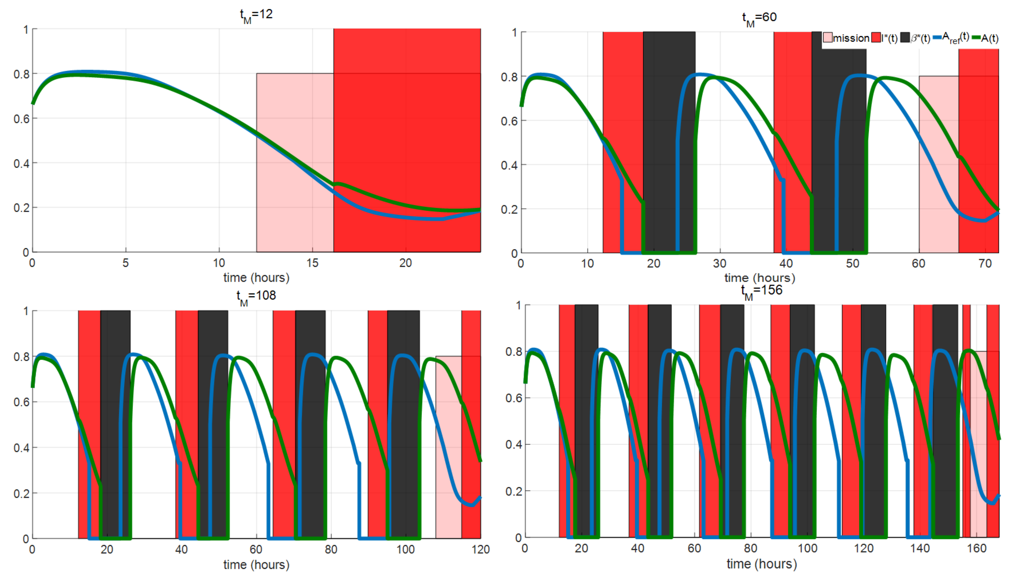
2.1. Mission Alertness Optimization

Inspired by the study in [20], we propose the mission alertness optimization problem, that is, to improve the subjective alertness during certain mission periods by optimizing the light exposure and sleep schedule in advance. Note that before the mission time, the subject can partially adapt his sleep schedule instead of following the spontaneous sleep schedule in Equation (7). This sleep schedule, with tunable sleep and wake times, is called the tunable sleep schedule in this paper. The sleep state in the tunable sleep schedule is expressed as

$$\beta \left(t\right)=F_{\beta }^{\prime }(t,\beta \left(t^{-}\right))=\left\{\begin{array}{cc}1,& t\in \{t_{\mathrm{sleep}}^1,\dots ,t_{\mathrm{sleep}}^{N_f}\},\\ 0,& t\in \{t_{\mathrm{wake}}^1,\dots ,t_{\mathrm{wake}}^{M_f}\},\\ \beta \left(t^{-}\right),& \mathrm{else},\end{array}\right.$$

(14)

with sleep and wake times constraint as

$$\begin{array}{c}{H}_m\le \Phi \left(t_{\mathrm{sleep}}^i\right)\le {\Phi }_{1max},L_m\le \Phi \left(t_{\mathrm{wake}}^j\right)\le {\Phi }_{2max},\end{array}$$

(15)

where $t_{\mathrm{sleep}}^i$ and $t_{\mathrm{wake}}^j$ are the ith sleep time and jth wake time, $M_f$ and $N_f$ are the total sleep and wake time from the beginning time of circadian regulation to the start of mission. $\Phi \left(t_{\mathrm{sleep}}^i\right)\ge H_m$ and $\Phi \left(t_{\mathrm{wake}}^j\right)\ge L_m$ indicate the subject cannot fall asleep earlier than the spontaneous sleep time or wake up later than the spontaneous wake time. Meanwhile, the inequality condition $\Phi \left(t_{\mathrm{sleep}}^i\right)>H_m$ is used to simulate the cases in our daily lives that we may fall asleep later than normal sleep times, as a result of night-shift, personal reasons or other external disturbance. $\Phi \left(t_{\mathrm{wake}}^i\right)>L_m$ corresponds to the cases where we may wake up earlier than spontaneous wake times by setting a morning alarm. $\Phi \left(t_{\mathrm{sleep}}^i\right)\le {\Phi }_{1max}$ and $\Phi \left(t_{\mathrm{wake}}^j\right)\le {\Phi }_{2max}$ are introduced, which were ignored in [20] and led to 40-h continuous wakefulness, as extra constraints to avoid excessive long wake duration and guarantee the daily sleep duration. The upper thresholds ${\Phi }_{1max}$ and ${\Phi }_{2max}$ could be set based on personal sleep habits. Individuals show various sleep types with daily sleep duration varying from 6 to 9 h [27]. In this paper, we choose these values ${\Phi }_{1max}=0.77$ and ${\Phi }_{2max}=0.27$, with sleep propensity at sleep and wake times shown as the red region in Figure 3, as an example to show that appropriately tuning the sleep schedule could improve cognitive performance without dramatically shortening the daily sleep duration.

Mission Alertness Optimization Problem: Given the initial value of state

$$\xi \left(0\right)={\xi }_0,$$

(16)

the state equation of the three-process model expressed as

$$\dot{\xi }=F(\xi ,I,\beta ),$$

(17)

and the tunable sleep schedule in Equation (14), the mission alertness optimization problem is formulated as

$$\begin{array}{c}maximize{\int }_{t_M}^{t_f}A\left(t\right)dt\left(\mathrm{or}minimize{\int }_{t_M}^{t_f}-A\left(t\right)dt\right),\end{array}$$

(18)

which subjects to the light intensity constraint $0\le I\left(t\right)\le I_{\max }$, sleep state during mission $\beta \left(t\right)=0$ between $t_M$ and $t_f$, sleep time constraints before mission $0.67\le \Phi \left(t_{\mathrm{sleep}}^i\right)\le 0.77$, $\forall i\in \{1,\dots ,N_f\}$, and wake time constraints before mission $0.17\le \Phi \left(t_{\mathrm{wake}}^j\right)\le 0.27$, $\forall j\in \{1,\dots ,M_f\}$. $t_M$ is the beginning time of the mission and $t_f$ is the final time of the mission. The initial state in Equation (16) is defined based on the periodic solution ${\xi }_{\mathrm{ref}}\left(t\right)$. $I_{max}$ is the maximum light intensity used before and during the mission. In practical use, the light intensity constraint could be set as a time-varying constraint, i.e., $0\le I\left(t\right)\le I_{max}\left(t\right)$, with $I_{max}\left(t\right)$ valued based on personal preference, health care, work demand, specifications of lighting equipment and other limits. For simplicity and to show the potential of using light to improve alertness, we set $I_{max}$ as a constant in this and following optimization problems in Section 2.2 and Section 2.3.

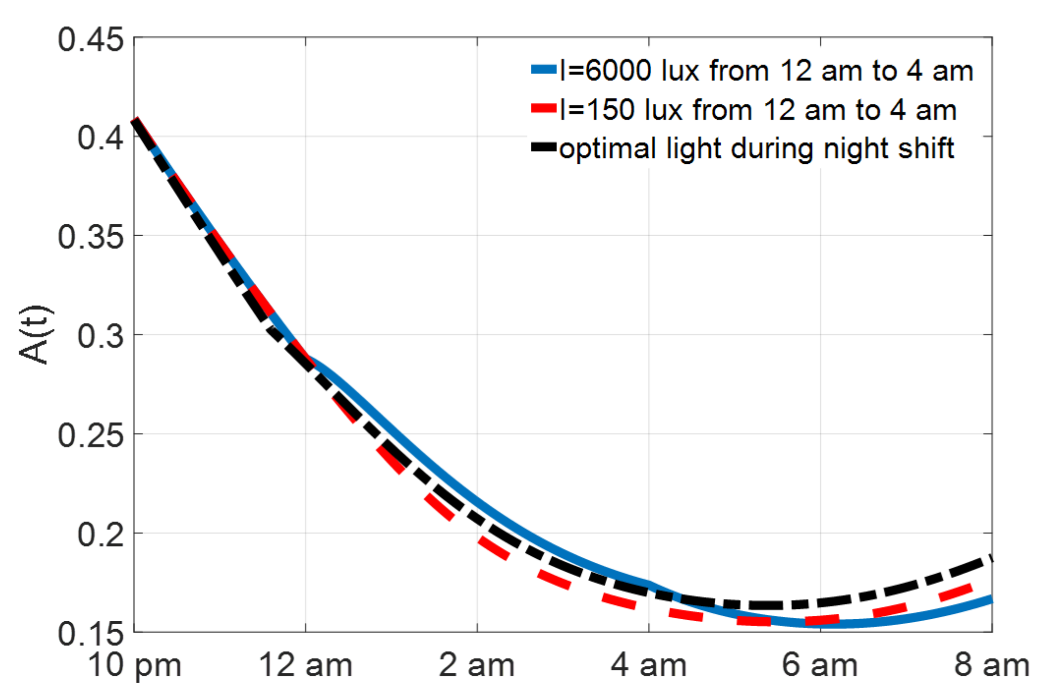
2.2. Night-Shift Alertness Optimization

As mentioned in Section 1, the nighttime light has great impacts on the alertness level of night-shift workers. Based on the experimental protocol in [19], the night-shift takes place between 10 pm and 8 am. We simulate two cases of this night-shift work: (1) A night-shift worker remains under a bright light $I=6000$ lux between 12 am and 4 am and stays under dim light with 150 lux for the rest of the night shift; (2) A night-shift worker stays under 150 lux dim light during the whole night-shift. The simulation results of these two cases are shown as the blue and red curves in Figure 6. The alertness level of the shift worker in the first case is larger during the interval between 1 am and 6 am. This result is consistent with the experimental results in [19] and implies that timed exposure to bright light during the night shift partially improves alertness.

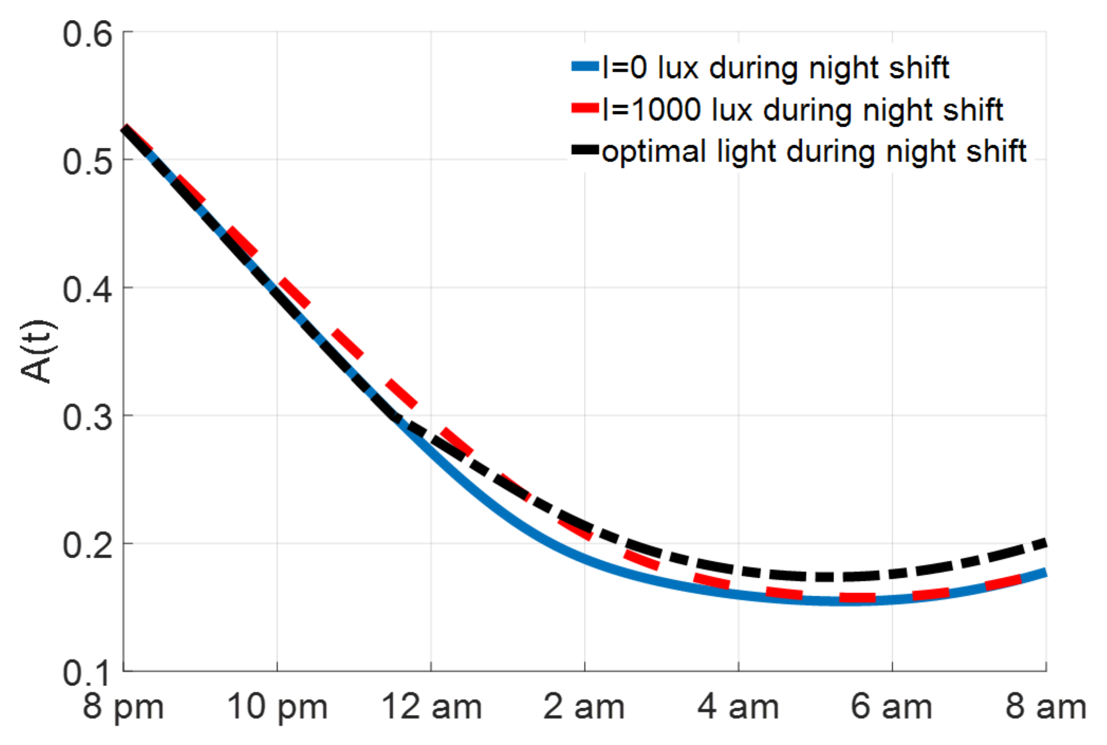
A similar experimental study of lighting impacts on night-shift alertness has been shown in [4], where the experimental subjects were divided into three groups. One stayed in the darkness, one was given bright light of 1000 lux, and one wore circadian light-blocking goggles between 8 pm and 8 am. The circadian light-blocking goggles filter out all light spectrum with the wavelength less than 480 nm. The experimental results indicate that the alertness levels of the group with the goggles are very close to those of the group that stayed in darkness. After blocking the short-wavelength light, the equivalent light intensity for the circadian rhythm of night-shift workers is 0 lux. Based on the experiments, we simulate two cases in shift work: the first worker stays in darkness (or wears goggles) with $I=0$ lux during the whole night-shift from 8 pm to 8 am, the second case stays under the bright light of $I=1000$ lux during this night-shift. Both simulation results in Figure 7 and experimental results in [4] show that, for the case in darkness during the night-shift, alertness decreases more rapidly in the first several hours of the night-shift, but is slightly larger than the case in bright light at the end of the night-shift.

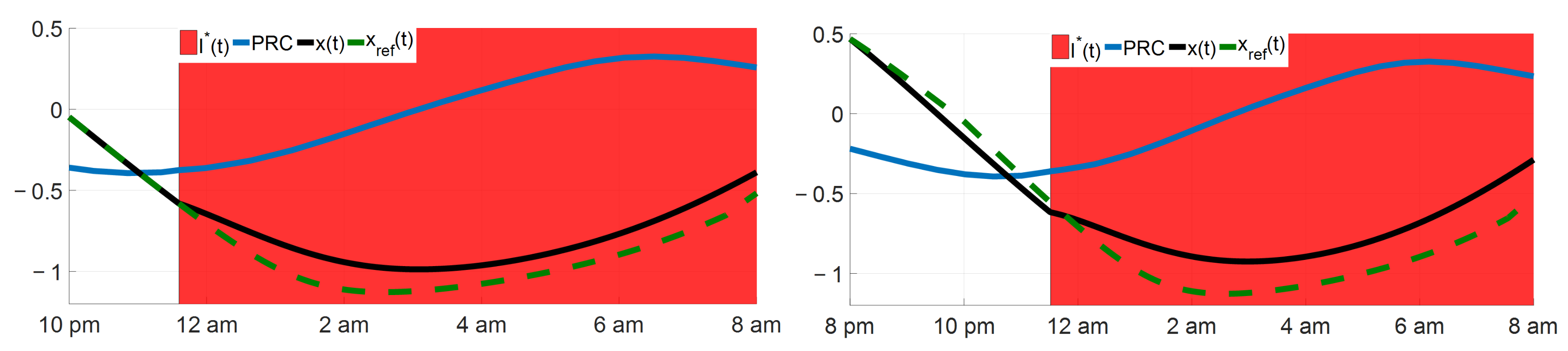
Based on these experimental studies, we formulate a night-shift alertness optimization problem, given as below:

Night-shift Alertness Optimization Problem: Given the initial condition in Equation (16), system dynamics in (17), the optimal light input is determined to maximize the cumulative alertness level during the night-shift. This optimization problem is formulated in the following form:

$$\begin{array}{c}maximize{\int }_0^{t_f}A\left(t\right)dt\left(\mathrm{or}minimize{\int }_0^{t_f}-A\left(t\right)dt\right)\end{array}$$

(19)

subjects to the light input constraint $0\le I\left(t\right)\le I_{\max }$, sleep state $\beta \left(t\right)=0$ between 0 and $t_f$, where $t=0$ corresponds to the beginning of the night-shift, $t_f$ is the final time of the night-shift.

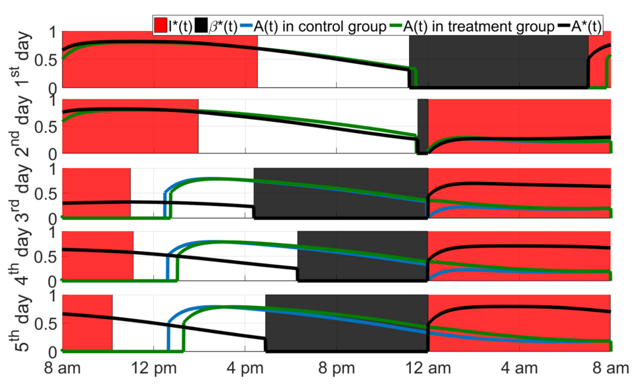
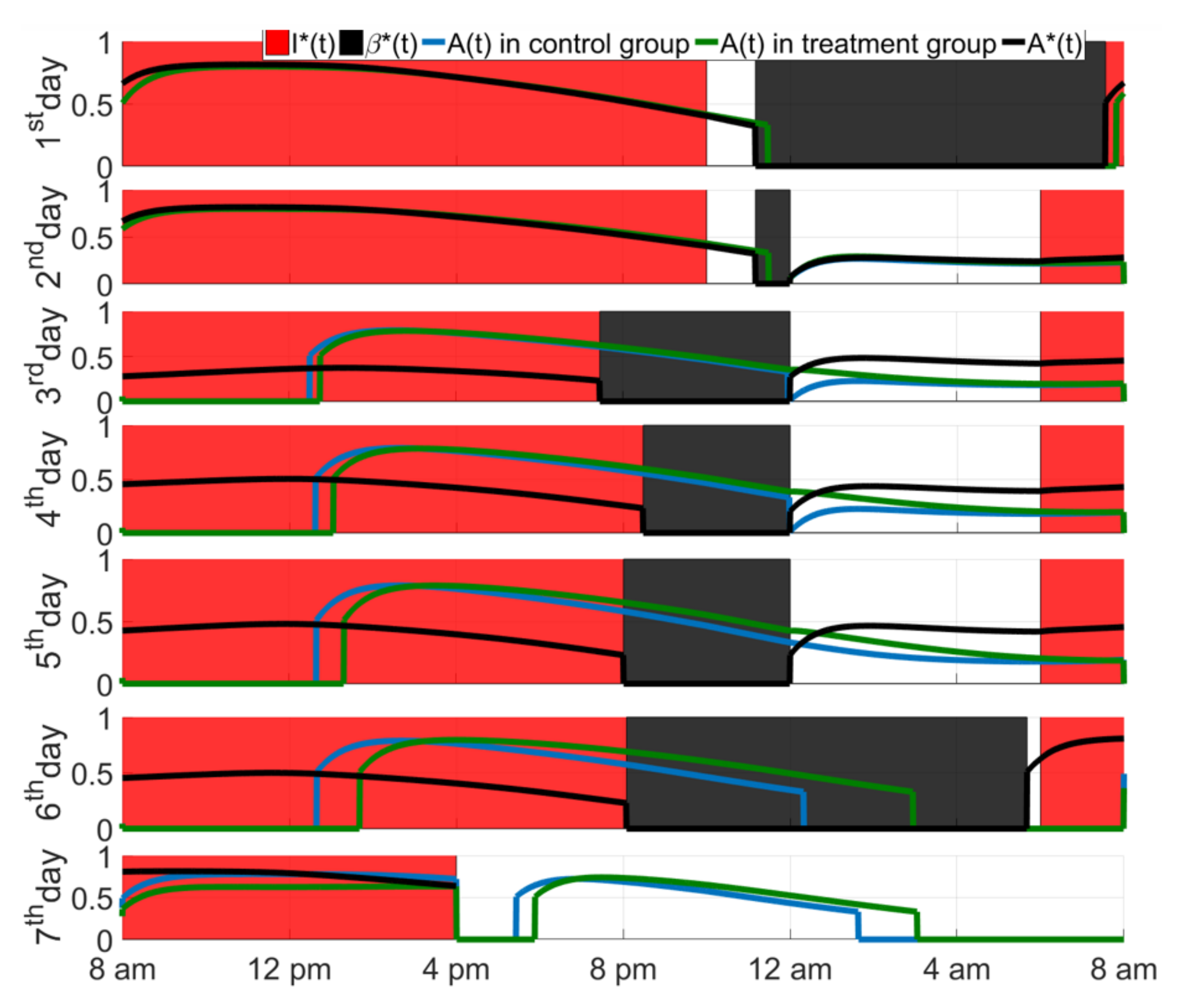
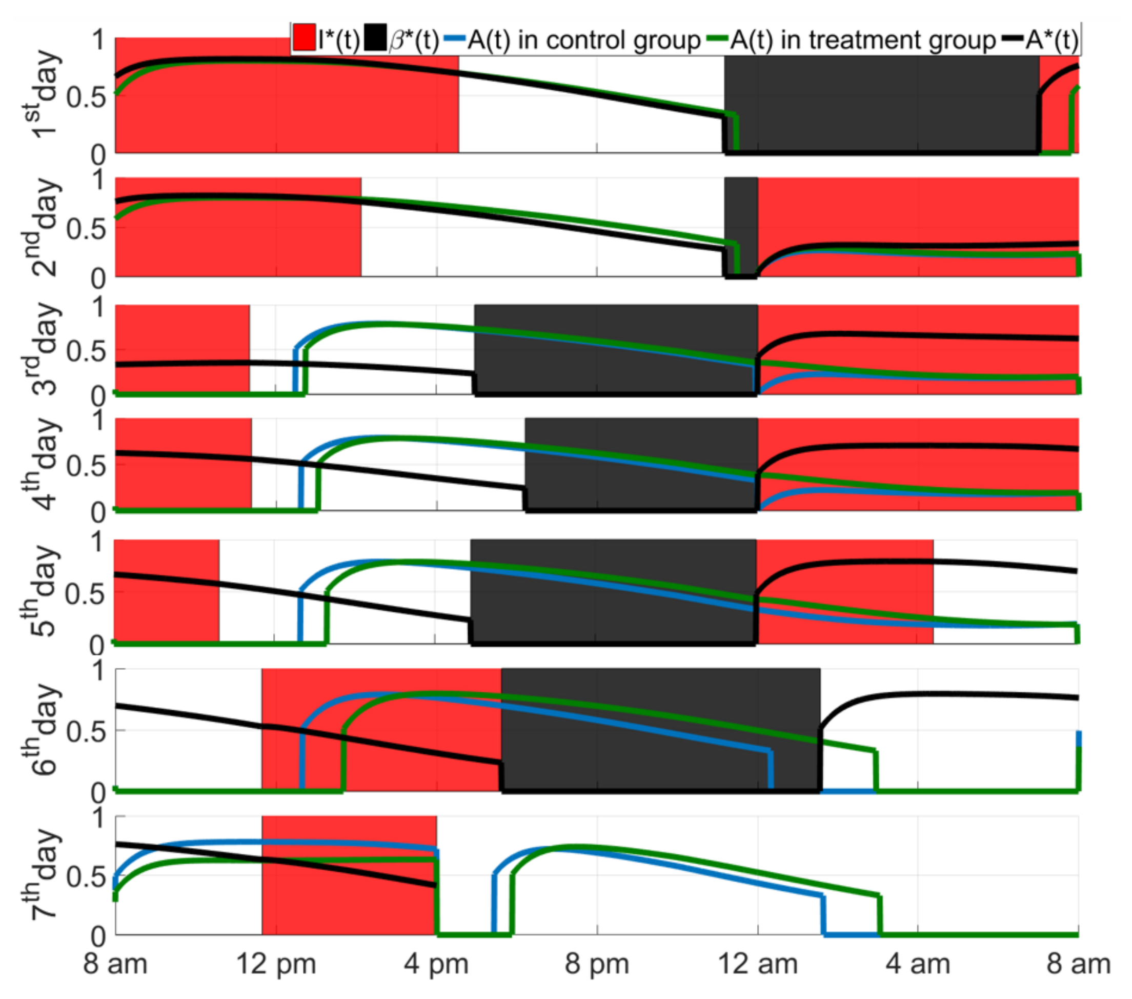
2.3. Consecutive Night-Shift Alertness Optimization

Another case considered in this paper comes from the experimental studies in [28]: These experimental studies asked subjects to remain awake for several consecutive night-shifts and investigated the cognitive impairments in days following night-shifts. These subjects were separated into two groups: control group and treatment group. In the control group, the subjects were assigned ordinary indoor light with 150 lux during the second through fifth nights, while the subjects in the treatment group received bright light with 7000∼12,000 lux. This experiment showed exposure to bright light during several consecutive night-shifts led to a significant shift (about 9 h) in the patterns of core body temperature and subjective assessment of alertness, but could result in serious cognitive impairments in the following day-shift. In this case, we determine the optimal light input and sleep schedule to maximize the cumulative (or average) alertness during either the consecutive night-shifts or the day after these night-shifts, or both of them.

Consecutive Night-shift Alertness Optimization Problem: Given the boundary condition in Equation (16), the system dynamics in Equation (17), and the tunable sleep schedule in Equation (14), we calculate the optimal light input and sleep schedule by solving the consecutive night-shift alertness optimization problem, formulated as below:

$$\begin{array}{c}maximize{C}_1·{\int }_{t\in T_{\mathrm{night}}}A\left(t\right)dt+C_2·{\int }_{t\in T_{\mathrm{day}}}A\left(t\right)dt,\end{array}$$

(20)

which subjects to the light input constraint $0\le I\left(t\right)\le I_{\max }$, the sleep state during shift working time $\beta \left(t\right)=0\mathrm{when}t\in T_{\mathrm{night}}\cup T_{\mathrm{day}}$, sleep time constraints outside the shift working time $0.67\le \Phi \left(t_{\mathrm{sleep}}^i\right)\le 0.77,\forall i\in \{1,\dots ,N_f\}$, and wake time constraints outside the shift working time $0.17\le \Phi \left(t_{\mathrm{wake}}^j\right)\le 0.27,\forall j\in \{1,\dots ,M_f\}$. $T_{\mathrm{night}}$ represents the set of all night-shift working periods and $T_{\mathrm{day}}$ represents the day-shift period this week. The positive constant $C_1$ and $C_2$ represent the weight of alertness during night-shifts and the day-shift in the objective function.

3. Solution Strategies and Algorithms

We apply the variational calculus and functional gradient descent algorithms to solve the alertness optimization problems proposed in the previous section. Equation (5) indicates that, in the three-process model, the state $\xi \left(t\right)$ follows different dynamics when the subject is sleeping ($\beta =1$) and awake ($\beta =0$). Therefore, the alertness optimization problems should be solved on a hybrid dynamical system with two kinds of modes: sleep mode and wake mode. The dynamics of the hybrid dynamical system in the ith mode are expressed in the following form:

$$\dot{\xi }=F_i(\xi ,I),t\in [t_{i-1},t_i),\forall i\in \{1,2,\cdots ,N\},$$

(21)

where N is the total number of modes, $t_N=t_f$ is the final time and $t_0=0$. Assume that the sleep-wake switching time $t_i,\forall i\in [1,\dots ,N-1]$ follows the constraint given in the following form:

$$t_i\in {\Omega }_{ti},\forall i\in \{1,\dots ,N-1\},$$

(22)

where ${\Omega }_{ti}$ represents the feasible region of switching time based on problem formulation. It could be defined based on the constraint of the switching condition in Equation (15) and the sleep and wake time constraints in the problem formulation. We formulate the objective cost function as

$$J={\int }_0^{t_f}L(t,\xi ,I)dt,$$

(23)

where the integrand $L(t,\xi ,I)$ maps $(t,\xi (t),I(t\left)\right)$ into a scalar. To include the constraints of the dynamical system in Equation (21) into the cost function, we introduce the Lagrange multipliers $\lambda \left(t\right)\in {\mathbb{R}}^5$ and formulate the augmented cost function as

$$J_a={\int }_{t_0}^{t_N}L(\tau ,\xi ,I)d\tau +\sum _{i=1}^N{\int }_{t_{i-1}}^{t_i}{\lambda }^T(\tau )·\left[F_i(\xi ,I)-\dot{\xi }(\tau )\right]d\tau .$$

(24)

To determine the extreme value of the cost function, we add perturbation terms of $\alpha \delta t_i$ and $\alpha \delta I$ into the switching time $t_i$ and light $I\left(t\right)$, respectively, resulting in perturbed state $\xi +\alpha \delta \xi +o(\alpha )$ and a perturbed augmented cost function, given as

$$\begin{array}{l}{J}_a+\alpha \delta J_a+o(\alpha )={\int }_{t_0}^{t_N}L(\tau ,\xi +\alpha \delta \xi +o(\alpha ),I+\alpha \delta I)d\tau \\ +{\displaystyle \sum _{i=1}^N}{\int }_{t_{i-1}+\alpha \delta t_{i-1}}^{t_i+\alpha \delta t_i}{\lambda }^T(\tau )·\left[F_i(\xi +\alpha \delta \xi +o(\alpha ),I+\alpha \delta I)-\dot{\xi }(\tau )-\alpha \delta \dot{\xi }(\tau )-o(\alpha )\right]d\tau .\end{array}$$

(25)

where $\alpha$ is a small scalar, $o(\alpha )$ represents a higher order term of $\alpha$. $\delta \xi$ and $\delta J_a$ represent first-order (linear) variations of $\xi$ and $J_a$ in $\delta I$ and $\delta t_i$, given as

$$\delta \xi =\underset{\alpha \to 0}{lim}\frac{\xi (I\left(t\right)+\alpha \delta I\left(t\right),t_i+\alpha \delta t_i)-\xi (I\left(t\right),t_i)}{\alpha },$$

$$\delta J_a=\underset{\alpha \to 0}{lim}\frac{J_a(I\left(t\right)+\alpha \delta I\left(t\right),t_i+\alpha \delta t_i)-J_a(I\left(t\right),t_i)}{\alpha }.$$

We subtract cost function in Equation (25) by (24) and take first-order variation of the augmented cost by dividing their difference by $\alpha$ and taking its limit with $\alpha \to 0$, then the first-order variation of the augmented cost is given explicitly as

$$\begin{array}{cc}\hfill \delta J_a=& {\int }_{t_0}^{t_N}{\left[\frac{\partial L(\tau ,\xi ,I)}{\partial \xi }\right]}^T\delta \xi +\frac{\partial L(\tau ,\xi ,I)}{\partial I}\delta Id\tau \hfill \\ \hfill +& \sum _{i=1}^N{\int }_{t_{i-1}}^{t_i}\left\{{\dot{\lambda }}^T\delta \xi +{\lambda }^T(\tau )\left[{\left(\frac{\partial F_i(\xi ,I)}{\partial \xi }\right)}^T\delta \xi +\frac{\partial F_i(\xi ,I)}{\partial I}\delta I\right]\right\}d\tau \hfill \\ \hfill -& \sum _{i=1}^N[{\lambda }^T\left(t_i^{-}\right)\delta \xi \left(t_i^{-}\right)-{\lambda }^T\left(t_{i-1}^{+}\right)\delta \xi \left(t_{i-1}^{+}\right)]\hfill \\ \hfill +& \sum _{i=1}^{N-1}[{\lambda }^T\left(t_i^{-}\right)F_i(\xi \left(t_i^{-}\right),I\left(t_i^{-}\right))-{\lambda }^T\left(t_i^{+}\right)F_{i+1}(\xi \left(t_i^{+}\right),I\left(t_i^{+}\right))]\delta t_i\hfill \\ \hfill +& \sum _{i=1}^{N-1}[L(t_i^{-},\xi \left(t_i^{-}\right),I\left(t_i^{-}\right))-L(t_i^{+},\xi \left(t_i^{+}\right),I\left(t_i^{+}\right))]\delta t_i.\hfill \end{array}$$

The selection of Lagrange multipliers $\lambda \left(t\right)$ does not affect the result of the augmented cost function. We choose $\lambda \left(t\right)$ in the following forms to offset terms of $\delta \xi$ in $\delta J_a$:

$$\lambda \left(t_N\right)=0,$$

(26)

$$\dot{\lambda }\left(t\right)=-\frac{\partial L(t,\xi ,I)}{\partial \xi }-{\left(\frac{\partial F_i(\xi ,I)}{\partial \xi }\right)}^T·\lambda \left(t\right)\mathrm{when}t\in [t_{i-1},t_i).$$

(27)

$${\lambda }_j\left(t_i^{-}\right)={\lambda }_j\left(t_i^{+}\right),j=\{1,2,3,4\},$$

(28)

$${\lambda }_5\left(t_i^{-}\right)=\left\{\begin{array}{cc}0,& t_i\mathrm{is}\mathrm{a}\mathrm{wake}\mathrm{time},\\ {\lambda }_5\left(t_i^{+}\right),& t_i\mathrm{is}\mathrm{a}\mathrm{sleep}\mathrm{time},\end{array}\right.$$

(29)

where ${\lambda }_j$ represents the multiplier of the jth state in $\xi$. As $n\left(t\right)$, $x\left(t\right)$, $x_c\left(t\right)$, $H\left(t\right)$ are all continuous at all switching times, i.e., $\delta {\xi }_j\left(t_i^{-}\right)=\delta {\xi }_j\left(t_i^{+}\right)$ for j={1,2,3,4}, then we have Equation (28). The sleep inertia $W\left(t\right)$ is reset to 0.32 and discontinuous at wake times, as mentioned in Section 2. We set the multiplier value ${\lambda }_5\left(t\right)$ follows (29) with $\delta {\xi }_5\left(t_i^{+}\right)\ne \delta {\xi }_5\left(t_i^{-}\right)=0$ at wake times, which will be used in backward simulation of Equation (27). After some simplifications, the first-order variation of the augmented cost function with respect to $\delta I$ and $\delta t_i$ is given as

$$\delta J_a{|}_{I,t_1,\dots ,t_{N-1}}=\sum _{i=1}^N{\int }_{t_{i-1}}^{t_i}\left[\frac{\partial L(t,\xi ,I)}{\partial I}+{\lambda }^T(\tau )·\frac{\partial F_i(\xi ,I)}{\partial I}\right]\delta Idt$$

$$+\sum _{i=1}^{N-1}\left[L(t_i^{-},\xi \left(t_i^{-}\right),I\left(t_i^{-}\right))-L(t_i^{+},\xi \left(t_i^{+}\right),I\left(t_i^{+}\right))+{\lambda }^T\left(t_i^{-}\right)·F_i(\xi \left(t_i^{-}\right),I\left(t_i^{-}\right))\right.$$

$$\left.-{\lambda }^T\left(t_i^{+}\right)·F_{i+1}(\xi \left(t_i^{+}\right),I\left(t_i^{+}\right))\right]\delta t_i,$$

This equation implies the linear variation of the augmented cost function resulting from a small perturbation in light input and switching times. As the cost function J is equal to $J_a$ with (21) satisfied, the gradients of J with respect to I and $t_i$ are given as

$${\nabla }_{I\left(t\right)}J=\frac{\partial L(t,\xi ,I)}{\partial I}+{\lambda }^T\left(t\right)·\frac{\partial F_i(\xi ,I)}{\partial I},$$

(30)

$$\begin{array}{cc}{\nabla }_{t_i}J=\hfill & L(t_i^{-},\xi \left(t_i^{-}\right),I\left(t_i^{-}\right))-L(t_i^{+},\xi \left(t_i^{+}\right),I\left(t_i^{+}\right))+{\lambda }^T\left(t_i^{-}\right)·F_i(\xi \left(t_i^{-}\right),I\left(t_i^{-}\right))\hfill \\ \hfill & -{\lambda }^T\left(t_i^{+}\right)·F_{i+1}(\xi \left(t_i^{+}\right),I\left(t_i^{+}\right)).\hfill \end{array}$$

(31)

Based on the gradient descent method, if we represent the light input and ith switching time at the jth iteration as $I^j\left(t\right)$ and $t_i^j$, their values can be updated by:

$$I^{j+1}\left(t\right)=min(max(0,I^j\left(t\right)-{\eta }_I·{\nabla }_{I\left(t\right)}J),I_{max}),$$

(32)

$$t_i^{j+1}=t_i^j-{\eta }_{\mathrm{switch}}·{\nabla }_{t_i^j}J\in {\Omega }_{t_i},$$

(33)

where ${\eta }_I$ and ${\eta }_{\mathrm{switch}}$ are the updating steps for light input and wake/sleep time and determined by a line search in the simulation. It should be guaranteed in the gradient descent process that $t_i$ satisfies the constraints in the problem formulation. Steps of the proposed gradient descent process in the calculation of the optimal light and sleep schedule for alertness optimization are listed below:

Step 1: Set $j=0$ and choose an initial guess of the light input $I^0\left(t\right)$ and the sleep schedule ${\beta }^0\left(t\right)$ (i.e., $t_i^0,i\in \{1,\dots ,N-1\}$);

Step 2: Integrate the state equation in (21) forward and determine the state ${\xi }^j\left(t\right)$, alertness $A^j\left(t\right)$, and objective function value $J^j$;

Step 3: Integrate (27) backward with the terminal condition in (26), using switching conditions in (28), (29) at switching times, to get ${\lambda }^j\left(t\right),t\in [t_0,t_f]$;

Step 4: Determine the gradient of the objective function to $I^j\left(t\right)$ and the sleep/wake times $t_i^j,i\in \{1,\dots ,N-1\}$ based on Equations (30) and (31), update $I^j$ and $t_i^j$ based on Equations (32) and (33);

Step 5: Increment j by 1. Repeat from Step 2 until $j=100$ or

$$I^j\left(t\right)=I^{j-1}\left(t\right)\mathrm{and}{\beta }^j\left(t\right)={\beta }^{j-1}\left(t\right).$$

We define the cost function in (23) as $L=-A$, and set the dynamics in (21) based on the three-process model. The stable solutions of this algorithm, denoted as $I^{*}\left(t\right)$ and ${\beta }^{*}\left(t\right)$, correspond to the optimal light input and sleep schedules that maximize the alertness. As discussed in [10,11], the optimal light in circadian regulation is bang-off control without singular regions, i.e., $I^{*}\left(t\right)=0$ or $I_{max}$ for $\forall t$. In the following figures, we use red regions to demonstrate the optimal light exposure time.

4. Numerical Implementation

4.1. Mission Alertness Optimization

In the mission alertness optimization problem formulated in Section 2.1, we optimize both light input before and during the mission, and sleep schedule before the mission. In our simulation, we set that the mission period begins at 8 pm and ends at 8 am in the next morning, i.e., $t_f-t_M=12$ h. The beginning time of the mission $t_M$, representing how many hours the subject has before the mission begins, can be set based on practical situations. We gradually increase the value of $t_M$ to investigate the impacts of the time length used for regulation in advance on the optimal cumulative alertness that can be reached during the mission. For each value of $t_M$, we use the solution algorithm in Section 3 to determine the optimal light $I^{*}\left(t\right)$ and sleep schedule ${\beta }^{*}\left(t\right)$. Here, we study two maximum light intensities, $I_{max}=1000$ lux (indoor light) and $I_{max}$ = 10,000 lux (outdoor bright light).

Table 2. The optimal cumulative alertness during the mission with different $t_M$. The row ’Reference’ means only reference light in Equation (11) and spontaneous sleep schedule are used before mission without light and sleep optimization. The values in bracket give average subjective alertness in VAS with a unit of mm.

${\mathit{t}}_{\mathit{M}}$	${\mathit{I}}_{max}=1000$ lux	${\mathit{I}}_{max}$ = 10,000 lux
Reference	3.04 (44.63)	3.04 (44.63)
12	3.42 (46.73)	3.49 (47.13)
36	3.87 (49.22)	4.15 (50.76)
60	4.69 (53.73)	5.39 (57.58)
84	5.58 (58.58)	6.47 (63.48)
108	6.48 (63.55)	7.39 (68.52)
132	7.31 (68.07)	7.92 (71.43)
156	7.85 (71.04)	8.13 (72.59)

shows the reference alertness level (under reference light described in Equation (11)) and optimal alertness level with various $t_M$ and light intensities. The optimal alertness level during a mission monotonically increases with the mission beginning time $t_M$, which is obvious that the earlier the subject starts the sleep regulation and light-based entrainment, the higher alertness performance he can reach during the mission. If the subject only uses the reference light-dark cycle with the spontaneous sleep schedule before the mission, the average alertness level in VAS during the mission is about 44.63 mm, while this scale is increased to 72.59 mm after optimizing light exposure and appropriately scheduling sleep one week in advance with $I_{max}$ = 10,000 lux. The comparison of alertness results with $I_{max}$ = 10,000 lux and those with $I_{max}=1000$ lux in Table 2 shows the alertness can be enhanced by using brighter light before and during the mission. The optimal results in Figure 8 indicate that the subject stays under a bright light in the evening (about 6 h before sleep) and slightly delays daily sleep times while maintaining the daily wake times before the mission. Light exposure during the evening and delayed sleep time both delay the circadian rhythm and the moments of peak alertness, finally making the subject feel less sleepy and relieving cognitive impairments during the mission period. Note sleep durations in optimal sleep schedules are all around 7–9 h, proving the tunable sleep schedule with constraints in (15) guarantees adequate daily sleep time.

4.2. Night-Shift Alertness Optimization

We study two alertness optimization cases of night-shift workers here. The first case has a night-shift from 10 pm to 8 am as in [19], i.e., the initial condition in Equation (16) is given as $\xi \left(0\right)={\xi }_{\mathrm{ref}}\left(16\right)$ and final time $t_f=10$. The second case has a night-shift from 8 pm to 8 am [4] with initial condition $\xi \left(0\right)={\xi }_{\mathrm{ref}}\left(14\right)$ and final time $t_f=12$. The maximum light intensities used in these two cases are both $I_{max}=1000$ lux. The solution algorithm in Section 3 is applied in these two cases without updating the sleep schedule. The optimal lights $I^{*}\left(t\right)$ are plotted in Figure 9 and the corresponding maximum alertness during two night-shifts are plotted as black dashed curves in Figure 6 and Figure 7. Numerical simulation shows the alertness is improved by exposure to light from about 11:30 pm to 8 am in these two cases. For the night-shift from 10 pm to 8 am, the average subjective alertness in VAS is 42.60 mm with optimal light input with $I_{max}=1000$ lux, slightly larger than the average alertness with 6000 lux light between 12 am and 4 am (42.58 mm) and 150 lux during the whole night-shift (42.24 mm). In another case, the average subjective alertness is also slightly increased from 44.52 mm (with goggles) and 45.27 (1000 lux during the whole night shift) to 45.47 mm by optimizing the light input. Note that the night-shift alertness optimization problem with a night-shift between 8 pm and 8 am is equivalent to the mission alertness optimization problem with $t_M=0$ in Section 4.1. Compared with the results in Table 2, the alertness improvement in this section is much smaller. Optimizing the light and sleep schedule before night-shift has a larger impact on relieving cognitive impairments during night-shift than only optimizing the light during night-shift.

The optimal solutions in Figure 8 and Figure 9 suggest light exposure in the last several hours (from about 11:30 pm to 8 am) of night-shift. Based on the formulation of the three-process model, light input has no direct impact on sleep homeostasis and sleep inertia in this case as the subject keeps awake during the whole night-shift. Light affects the alertness level through the Process C, i.e., the circadian state x. We plotted the state x under optimal light, the reference state $x_{\mathrm{ref}}$, and the phase response curve (PRC) of the Process C [11] in Figure 9. The value of alertness $A\left(t\right)$ is proportional to $x\left(t\right)$, whose value grows with the light input from 11:30 pm to 8 am. The PRC value indicates the light between 11:30 pm to 3 am delays the circadian phase, which delays the process that x reaches its minimum value. While the light between 3 am and 8 am advances the circadian phase and boosts the state x increase rapidly. Therefore, the light between 11:30 pm to 8 am improves subjective alertness during the night-shift.

4.3. Consecutive Night-Shift Worker Alertness Optimization

For the consecutive night-shift alertness optimization problem, we set that the worker has four consecutive night-shifts between the second day and fifth day and a subsequent day-shift at the end (seventh day) of this week. The initial condition is given as

$$\xi \left(0\right)={\xi }_{\mathrm{ref}}\left(2\right),$$

that is, the light and sleep regulation process starts from 8 am on the first day of this week. The sets of night-shifts and day-shift in consecutive night-shift alertness optimization problem in Equation (20) is given as

$$T_{\mathrm{night}}=[40,48]\cup [64,72]\cup [88,96]\cup [112,120],$$

$$T_{\mathrm{day}}=[144,152],$$

which means the worker has night-shifts between 12 am and 8 am on the second to fifth days this week. The day-shift begins at 8 am and ends at 4 pm on the last day of this week. The light intensity we use here is $I_{\max }=10,000$ lux. Here, we study three different cases by changing the values of weights $C_1$ and $C_2$:

• Case 1:$C_1=1$ and $C_2=0$, that is, relieving fatigue and cognitive impairments only during night-shifts;
• Case 2:$C_1=0$ and $C_2=1$, i.e., improving cognitive performance in the day-shift after 4 consecutive night-shifts;
• Case 3:$C_1=1$ and $C_2=1$, i.e., improving the alertness in both consecutive night-shifts and the subsequent day-shift.

Firstly, we determine the optimal light and sleep schedule for Case 1 and plot them in Figure 10. For comparison, we use the three-process model to simulate the alertness of subjects in the control group and treatment group in [28] and also show them in Figure 10. The average alertness values in VAS during four night-shifts in the control group and treatment group are 41.40 mm and 44.70 mm, respectively. After light and sleep optimization, the average alertness is increased to 66.61 mm. The optimal light and sleep schedule in Figure 10 indicate exposure to 10,000 lux light in all four night-shifts. On the second night, the subject only falls asleep for a short period before the night-shift and the alertness level in this night-shift is close to those in the control and treatment group. However, in the following days, the subject has long sleep durations before night-shifts, and his alertness level is much higher than the control and treatment groups.

The solution to the alertness optimization problem in Case 2 is plotted in Figure 11. Compared with the results in Case 1, the optimal results in Figure 11 suggest the subject stays in darkness during most of the night-shifts, and has a long sleep duration (about 10 h) on the 6th day. The average alertness level between 8 am and 4 pm on the 7th day in the optimal result is 78.38 mm, higher than the average alertness in the control group (65.08 mm) and treatment group (70.79 mm), proving that appropriate tuning light and sleep schedule alleviate cognitive impairments in the day following consecutive night-shifts. The optimal results of Case 3 in Figure 12 suggest exposure to 10,000 lux light during the whole night-shifts in the 2nd to 4th days, but only receiving light in the first 4 h and keeping away from light in the last 4 h in the night-shift in the 5th day. On the 7th day, the subject keeps away from light in the first 4 h and stays under 10,000 lux in the last several hours in the day-shift. The optimal average alertness during all night-shifts and day-shift in this week is 67.35 mm, also dramatically larger than those in the control (48.62 mm) and treatment groups (49.61 mm).

The solutions of these cases reveal the process that light exposure and sleep schedule regulate humans’ alertness and cognitive performance: the bright light during night-shifts suppresses fatigue and improves alertness at the cost of circadian rhythm disruption, consistent with the previous conclusion in Section 4.1 and Section 4.2, while the optimal solution in Case 2 suggests the subject stay in darkness or wearing blocking goggles to avoid bright light to guarantee the normal circadian rhythm and alertness level could not be seriously disrupted by light during prior night-shifts, as discussed in [4]. Compared with Case 2, the longer sleeping duration before night-shifts in optimal solutions in Case 1 also boosts alertness during night-shifts. The solution of Case 3 in the first four days is almost the same as that of Case 1, while the optimal light and sleep schedule between the 5th and 7th-day show a difference from those in either Case 1 or Case 2, demonstrate a trade-off between the alertness in the last night-shift and day-shift.

5. Conclusions

This paper provides a three-process hybrid dynamic model for simulation of the time evolution of humans’ alertness and sleepiness under light exposure and sleep schedule. Calculus of variation is applied to the analysis of this model and alertness optimization problems are solved by the gradient descent algorithm proposed. The simulation of the three-process model demonstrates the process that the light and sleep schedule regulate cognitive performance. The solutions indicate that cognitive impairments during the night-shift and mission can be improved by optimized light exposure and appropriately tuning sleep schedule. The model and solution algorithms are new contributions to the field of circadian rhythmic dynamics and non-image-forming effects of light. They may be helpful in the application of light in health improvement, circadian rhythm regulation, and cognitive impairment relief.

References

1. Brainard, G.C.; Hanifin, J.P.; Greeson, J.M.; Byrne, B.; Glickman, G.; Gerner, E.; Rollag, M.D. Action spectrum for melatonin regulation in humans: Evidence for a novel circadian photoreceptor. J. Neurosci. 2001, 21, 6405–6412. [Google Scholar] [CrossRef] [PubMed] [Green Version]
2. Rahman, S.A.; Kollara, A.; Brown, T.J.; Casper, R.F. Selectively filtering short wavelengths attenuates the disruptive effects of nocturnal light on endocrine and molecular circadian phase markers in rats. Endocrinology 2008, 149, 6125–6135. [Google Scholar] [CrossRef] [PubMed]
3. Lockley, S.W.; Evans, E.E.; Scheer, F.A.; Brainard, G.C.; Czeisler, C.A.; Aeschbach, D. Short-wavelength sensitivity for the direct effects of light on alertness, vigilance, and the waking electroencephalogram in humans. Sleep 2006, 29, 161–168. [Google Scholar] [PubMed]
4. Rahman, S.A.; Marcu, S.; Shapiro, C.M.; Brown, T.J.; Casper, R.F. Spectral modulation attenuates molecular, endocrine, and neurobehavioral disruption induced by nocturnal light exposure. Am. J. Physiol. Endocrinol. Metab. 2011, 300, E518–E527. [Google Scholar] [CrossRef]
5. Asgari-Targhi, A.; Klerman, E.B. Mathematical modeling of circadian rhythms. Wires Mech. Dis. 2018, 11, e1429. [Google Scholar] [CrossRef]
6. Monga, B.; Moehlis, J. Optimal phase control of biological oscillators using augmented phase reduction. Biol. Cybern. 2019, 113, 161–178. [Google Scholar] [CrossRef]
7. Diekman, C.O.; Bose, A. Reentrainment of the circadian pacemaker during jet lag: East-west asymmetry and the effects of north-south travel. J. Theor. Biol. 2018, 437, 261–285. [Google Scholar] [CrossRef]
8. Booth, V.; Xique, I.; Behn, C.G.D. One-dimensional map for the circadian modulation of sleep in a sleep-wake regulatory network model for human sleep. SIAM J. Appl. Dyn. Syst. 2017, 16, 1089–1112. [Google Scholar] [CrossRef]
9. Abel, J.H.; Doyle, F.J. A systems theoretic approach to analysis and control of mammalian circadian dynamics. Chem. Eng. Res. Des. 2016, 116, 48–60. [Google Scholar] [CrossRef] [Green Version]
10. Serkh, K.; Forger, D.B. Optimal schedules of light exposure for rapidly correcting circadian misalignment. PLoS Comput. Biol. 2014, 10, e1003523. [Google Scholar] [CrossRef]
11. Julius, A.A.; Yin, J.; Wen, J.T. Time optimal entrainment control for circadian rhythm. PLoS ONE 2019, 14, e0225988. [Google Scholar] [CrossRef]
12. Mallis, M.M.; Mejdal, S.; Nguyen, T.T.; Dinges, D.F. Summary of the key features of seven boimathematical models of human fatigue and performance. Aviat. Space Environ. Med. 2004, 75, A4–A14. [Google Scholar]
13. Daan, S.; Beersma, D.G.; Borbély, A.A. Timing of human sleep: Recovery process gated by a circadian pacemaker. Am. J. Physiol. 1984, 246, R161–R178. [Google Scholar] [CrossRef]
14. Skeldon, A.C.; Dijk, D.J.; Derks, G. Mathematical models for sleep-wake dynamics: Comparison of the two-process model and a mutual inhibition neuronal model. PLoS ONE 2014, 9, e103877. [Google Scholar]
15. Achermann, P.; Werth, E.; Dijk, D.J.; Borbely, A.A. Time course of sleep inertia after nighttime and daytime sleep episodes. Arch. Ital. Biol. 1995, 134, 109–119. [Google Scholar]
16. Achermann, P.; Borbély, A.A. Simulation of daytime vigilance by the additive interaction of a homeostatic and a circadian process. Biol. Cybern. 1994, 71, 115–121. [Google Scholar] [CrossRef]
17. Reifman, J.; Gander, P. Commentary on the three-process model of alertness and broader modeling issues. Aviat. Space Environ. Med. 2004, 75, A84–A88. [Google Scholar]
18. Pettersson, K.; Müller, K.; Tietäväinen, A.; Gould, K.; Hæggström, E. Saccadic eye movements estimate prolonged time awake. J. Sleep Res. 2019, 28, e12755. [Google Scholar] [CrossRef] [Green Version]
19. Dawson, D.; Campbell, S.S. Timed exposure to bright light improves sleep and alertness during simulated night shifts. Sleep 1991, 14, 511–516. [Google Scholar] [CrossRef] [Green Version]
20. Zhang, J.; Wen, J.T.; Julius, A.A. Optimal circadian rhythm control with light input for rapid entrainment and improved vigilance. In Proceedings of the Conference on Decision and Control (CDC), Maui, HI, USA, 10–13 December 2012; pp. 3007–3012. [Google Scholar]
21. Lowden, A.; Kecklund, G. Considerations on how to light the night-shift. Light. Res. Technol. 2021, 53, 437–452. [Google Scholar] [CrossRef]
22. Wehr, T.A. In short photoperiods, human sleep is biphasic. J. Sleep Res. 1992, 1, 103–107. [Google Scholar] [CrossRef]
23. Bes, F.; Jobert, M.; Schulz, H. Modeling napping, post-lunch dip, and other variations in human sleep propensity. Sleep 2009, 32, 392–398. [Google Scholar] [CrossRef] [Green Version]
24. Leeuwen, W.M.A.; Pekcan, C.; Barnett, M.; Kecklund, G. Mathematical modelling of sleep and sleepiness under various watch keeping schedules in the maritime industry. Mar. Policy 2021, 130, 104277. [Google Scholar] [CrossRef]
25. Akerstedt, T.; Gillberg, M. The circadian variation of experimentally displaced sleep. Sleep 1981, 4, 159–169. [Google Scholar] [CrossRef] [Green Version]
26. Johnson, M.P.; Duffy, J.F.; Dijk, D.J.; Ronda, J.M.; Dyal, C.M.; Czeisler, C.A. Short-term memory, alertness and performance: A reappraisal of their relationship to body temperature. J. Sleep Res. 1992, 1, 24–29. [Google Scholar] [CrossRef]
27. Piltz, S.H.; Behn, C.G.D.; Booth, V. Habitual sleep duration affects recovery from acute sleep deprivation: A modeling study. J. Theor Biol. 2020, 540, 110401. [Google Scholar] [CrossRef]
28. Czeisler, C.A.; Johnson, M.P.; Duffy, J.F.; Brown, E.N.; Ronda, J.M.; Kronauer, R.E. Exposure to bright light and darkness to treat physiologic maladaptation to night work. N. Engl. J. Med. 1990, 332, 1253–1259. [Google Scholar] [CrossRef]
Figure 1. (Upper panel) The periodic solution of the three-process model in Equations (1)–(5) and (8) with the reference light input in (11) and spontaneous sleep in (7). (Lower panel) The reference light-dark cycle I ref (red region), the corresponding spontaneous sleep schedule (grey region) and the alertness level A ( t ) (blue curve).
Mathematics 10 01916 g001
Figure 2. The recovery sleep duration to the duration of sleep deprivation after spontaneous sleep time. The blue symbols show the means and standard deviations of experimental data in [13] and the black nodes demonstrate the simulation results of the three-process model.
Mathematics 10 01916 g002
Figure 3. The time evolution of sleep propensity to the duration of sleep deprivation (valued as {0,1,…,24} h) beyond spontaneous sleep time. The red region demonstrated the feasible sleep propensity in tunable sleep schedule in following Equation (15). The black curves demonstrate the time evolution of simulated sleep propensity with various lengths of sleep deprivation. The blue curve plots the value of homeostasis at spontaneous wake times following sleep deprivation, i.e., L m + A c · x .
Mathematics 10 01916 g003
Figure 4. Comparison of predicted alertness from simulation results of the 60 h constant routine protocol with the subjective alertness data (mean ± SD) in [26]. The initial point 0 in the relative clock hour is referred to as the wake time. The predicted alertness A ( t ) in the three-process model has been scaled to fit the empirical units.
Mathematics 10 01916 g004
Figure 5. Comparison of simulation results and empirical data (mean ± SD) of sleepiness rating during a dim light constant routine protocol after a long (left) and a short (right) photoperiod schedule.
Mathematics 10 01916 g005
Figure 6. The alertness level of night-shift workers with light I = 6000 lux (blue solid line) and I = 150 lux (red dashed line) from 12 am to 4 am, and that with optimal light I * ( t ) during the whole night-shift (black dashed line, solved by the algorithms in Section 3). The cumulative alertness values (and the average subjective alertness in VAS) of these three strategies are 2.21 (42.58 mm), 2.17 (42.24 mm), and 2.22 (42.60 mm), respectively.
Mathematics 10 01916 g006
Figure 7. The alertness level of the night-shift workers with goggles (blue solid line), the bright light of 1000 lux (red dashed line), and optimal light I * ( t ) (black dashed line, solved by the algorithms in Section 3) from 8 pm to 8 am. The cumulative alertness (and the average subjective alertness in VAS) of these three cases are 3.02 (44.53 mm), 3.15 (45.27 mm), and 3.19 (45.47 mm), respectively.
Mathematics 10 01916 g007
Figure 8. Alertness optimization results with I max = 10,000 lux and various mission beginning time t M . The pink regions show the mission period, the red and black regions show the optimal light exposure and sleep durations. Blue and green curves plots the reference alertness under periodic light in Equation (11) and optimal alertness solved by the gradient descent method in Section 3.
Mathematics 10 01916 g008
Figure 9. Comparison of the circadian state x ( t ) (black solid line) under the optimal light I * ( t ) (red region) and the reference state x ref ( t ) (green dash line) in the night-shift from 10 pm to 8 am (left) and night-shift from 8 pm to 8 am (right). The blue line in each subfigure shows the PRC value of the CBT model.
Mathematics 10 01916 g009
Figure 10. The alertness optimization results in Case 1, where the red and black region show the optimal light I * ( t ) and sleeping period in β * ( t ) . The blue, green, and black curves demonstrate the alertness in the control group, treatment group, and optimal results.
Mathematics 10 01916 g010
Figure 11. The alertness optimization results in Case 2.
Mathematics 10 01916 g011
Figure 12. The alertness optimization results in Case 3.
Mathematics 10 01916 g012