Innovation of the Component GARCH Model: Simulation Evidence and Application on the Chinese Stock Market

Abstract

The component GARCH model (CGARCH) was among the first attempts to split the conditional variance into a permanent and transitory component. With the application to economic and finance data, it helps investigate the long- and short-run movements of volatility affecting securities. Like all GARCH-type models, the innovation series of the CGARCH are usually assumed to follow a Normal distribution, which cannot accommodate fat-tailed properties commonly present in empirical data. The resulting estimates are not efficient when a Normal assumption is employed. In this paper, we consider the tempered stable distribution, which has the attractive stability under aggregation property missed in other popular fat-tailed distributions such as Student’s t-distribution and General Error Distribution (GED). Through systematically designed simulation studies, our results demonstrate that a CGARCH model with tempered stable distribution uniformly outperforms those with Normal, Student’s t-distribution and GED. Our empirical study on the Shanghai Stock Exchange index also leads to the same conclusions. Therefore, we argue that the CGARCH model with tempered stable distribution could be widely used to model economic and financial data in general contexts, focusing on both the long- and short-run volatility behaviours.

1. Introduction

Over the past few decades, the finance research related to volatility modelling has produced a tremendous number of studies. Among numerous employed methodologies, the GARCH model proposed in the seminal work of [1] has become one of the most popular methods. Its popularity is largely due to the ability to capture characteristics of financial time series such as time-varying heteroskedasticity and volatility clustering [2]. Various extensions have been developed and widely used to investigate different features of finance time-series. In this research, we focus on the component GARCH (CGARCH) model studied in Engle and Lee [3]. The CGARCH model constitutes a convenient method of incorporating long-memory-like features into a short-memory model via fitting a permanent and transitory component within the GARCH framework.

Originally, all GARCH-type models are constructed based on the assumption that the financial time series follows a Normal (Gaussian) distribution. However, significant evidence suggests that the financial time series is rarely Gaussian, but typically leptokurtic, and exhibits heavy-tail behaviour [4,5,6,7]. Theoretically, GARCH model can accommodate for fat-tailedness through its specification [8]. In practice, however, there is still excess kurtosis left in the standardized residuals in most cases [9]. To solve this problem, a common solution is to employ a fat-tailed distribution such as the Student’s t-distribution or General Error Distribution (GED) [10,11,12,13]. Compared to the GARCH model with Normal distribution, estimates of which are believed to be consistent even when the true distribution is fat-tailed [8], a GARCH model with true distribution can lead to more efficient results [4].

Motivated by those studies, a CGARCH model with a fat-tailed distribution should always be employed in practical finance research. This is particularly important in accurately forecasting financial volatility, which is critical to portfolio risk-management such as measuring risks with Value-at-Risk and/or Conditional-Tail-Expectation. However, a recent study by Calzolari et al. [9] argues that the widely used Student’s t-distribution and GED are problematic. Their most outstanding drawback is that those distributions lack stability under aggregation, which is of particular importance in portfolio applications and risk management. This leaves the following question still open for academics and practitioners: which fat-tailed distribution should we use for the CGARCH model when the true distribution is unknown? We aim to address this with simulation and empirical evidence in the subsequent sections.

As a replacement of Student’s t and GED, the $\alpha$-stable distribution is recommended by Calzolari et al. [9], which has the stability-under-aggregation feature. Additionally, they argue that similar to the Student’s t and GED, $\alpha$-stable distribution can be easily adapted to account for many properties of volatility such as asymmetry in the underlying financial time-series. Unfortunately, since the second moment of $\alpha$-stable distribution does not exist in most cases, a GARCH model with this distribution will lead to problematic interpretation. Hence, the sought-after alternative distribution would be of particular interest for the application of a GARCH model.

The tempered stable distribution is a natural substitution of the $\alpha$-stable, and its effectiveness has been studied for various GARCH family models [14,15,16]. Firstly introduced (In this case, the associated Levy processes are called “truncated Levy flights”, the appropriateness of which for application in the GARCH model is also discussed in Constantinides and Savel’ev [17]) in Koponen [18], tempered stable distribution covers several well-known subclasses such as Variance Gamma distributions, bilateral Gamma distributions and CGMY distributions [19]. The advantage of this distribution is that it retains most of the attractive properties of the $\alpha$-stable distribution and has a defined second moment.

The application of tempered stable distribution in financial risk-management has become an important topic in existing research. In their influential work, Kim et al. [20] were among the first to employ tempered stable distribution within the GARCH modelling framework. Other earlier attempts include the application of modified tempered stable distribution [21], the discussion on tempered infinitely divisible GARCH model Kim et al. [22], proposition of numerical method for estimation [23], and others. More recently, tempered stable distribution has been systematically studied for influential extensions of GARCH models, such as the Markov Regime-switching GARCH [24], Fractionally Integrated GARCH Feng and Shi [16] and Asymmetric Power GARCH [25]. Over the past few years, Kim et al. [26] investigated the case with time-varying exponential tails, and Kurosaki and Kim [27] and Xia and Grabchak [28] focused on application of tempered stable distribution on the multivariate GARCH models.

In this paper, we explore the feasibility of classical tempered stable distribution (also known as the CTS distribution) for the CGARCH model and argue that it outperforms both the Gaussian and commonly used fat-tailed distributions (Student’s t and GED). To demonstrate this, we conduct a series of simulation studies to compare the performance of GARCH model with different distributions. First, we set the true distribution as Student’s t and GED, respectively. Via six combinations of different parameters and sample size, CGARCH models with Gaussian and three distinct fat-tailed distributions are systematically analysed. It is demonstrated that when the true distribution is Student’s t or GED, the CGARCH model with tempered stable distribution generates very similar results to that with true distribution. More importantly, it outperforms all the other competitors in terms of consistency, efficiency and overall performance. Second, we let the tempered stable be the true distribution. Six sets of simulations are further constructed, including different choices of CGARCH and tempered stable distribution parameters. In this scenario, none of the CGARCH models with Gaussian, Student’s t or GED distributions perform as well as that with the tempered stable.

To empirically compare the CGARCH model with different distributions, we apply them to the daily return of the Shanghai Stock Exchange index. The results suggest that the CGARCH model with tempered stable outperforms all the other competing alternatives, including a CGARCH model with Copula transformation, under various criteria. When in- and out-of-sample forecasting performance is analysed, CGARCH model produces the smallest forecasting error in both cases. Finally, comparing the fitted Value-at-Risk (VaR) among all models, we find that the two-sided 95% VaR produced by CGARCH model with tempered stable distribution is the least biased statistic.

The contributions of this paper are threefold. First, consistent with existing literature, our simulation evidence systematically demonstrates that the CGARCH model with the Gaussian distribution is consistent but not efficient, when the true distribution is not Normal. Second, if fitted incorrectly, we show that CGARCH model with the widely employed Student’s t and GED may introduce considerable biases. In contrast, the CGARCH model with tempered stable distribution can generate desirable results. Therefore, for a financial time-series with an unknown fat-tailed underlying distribution, the tempered stable should always be employed within a CGARCH framework. This finding satisfactorily answers our research question and significantly contributes to the existing literature. Finally, as evidenced by our empirical study, the CGARCH model with tempered stable distribution consistently outperforms all other competitors. For financial practitioners, our result implies that using the tempered stable distribution may largely increase the accuracy of their risk measures with the CGARCH model. This can further benefit their portfolio management and other enterprise risk-management issues, where accurate risk measure is the major concern.

The remainder of this paper proceeds as follows. Section 2 describes the specification of the CGARCH model. Section 3 explains how the Student’s t, GED and tempered stable distributions can be applied to the CGARCH model. We conduct three independent simulation studies in Section 4. The empirical results are discussed in Section 5. Section 6 concludes the paper.

2. CGARCH Model

The GARCH model is proposed in the seminal work of Bollerslev [1]. Because of its capability to capture some important characteristics of financial time-series (for example, time-varying heteroskedasticity and volatility clustering), extensions of the GARCH model have become a standard way of studying financial volatility [2]. In particular, the component GARCH (CGARCH) model developed by Engle and Lee [3] decomposes the conditional variance into a permanent and transitory component. This allows the investigation of the long- and short-run movements of volatility affecting securities in finance research. For the CGARCH(1,1) specification, we have that

$$\begin{array}{cc}\hfill r_t& =\mu +{\epsilon }_t\mathrm{where}{\epsilon }_t={\eta }_t\sqrt{h_t}\hfill \\ \hfill h_t& =q_t+s_t\hfill \\ \hfill s_t& =(\alpha +\beta )s_{t-1}+\alpha ({\epsilon }_{t-1}^2-h_{t-1})\hfill \\ \hfill q_t& =\omega +\rho q_{t-1}+\varphi ({\epsilon }_{t-1}^2-h_{t-1})\hfill \end{array}$$

(1)

where ${\epsilon }_t$ is the error at time t. ${\eta }_t$ is an identical and independent innovation sequence following a certain distribution, with zero mean and unit standard deviation. $h_t$ is the conditional variance of $r_t$ at time t, which is composed of a transitory component $s_t$ and a permanent component $q_t$. $\alpha +\beta$ and $\rho$ measure the autoregressive persistence of the transitory and permanent components, respectively. $\alpha$ and $\varphi$ stand for the immediate impacts of volatility shocks (${\epsilon }_{t-1}^2-h_{t-1}$) on the short- and long-run components, respectively. It is constrained $(\alpha +\beta )<\rho$ to distinguish between the two components. In other words, the persistence of $q_t$ should be stronger than that of $s_t$. Similarly, we let $\alpha \ge \varphi$, so that immediate impact of volatility shocks of the long-run component is smaller than that of the short-run component.

The stationarity and non-negative conditional variance conditions of the CGARCH model are straightforward. According to Engle and Lee [3], a CGARCH(1,1) process is stationary with non-negative $h_t$ if $1>\rho >(\alpha +\beta )>0$, $\beta >\varphi >0$, $\alpha >\varphi >0$ and $\omega >0$. Under such conditions, $h_t$ will converge to $\omega /(1-\rho )$ in the long run.

In order to estimate the parameters of the CGARCH model, Maximum Likelihood Estimation (MLE) is employed. Therefore, the series ${\eta }_t$ needs to follow a specific distribution. Originally, the CGARCH model is developed based on the Standard Normal (Gaussian) distribution. In other words, ${\eta }_t={\epsilon }_t/\sqrt{h_t}\sim N(0,1)$ (Since the mean of ${\epsilon }_t$ is 0, ${\eta }_t$ is sometimes named as standardized residual). Hence, the conditional density of ${\epsilon }_t$ can be constructed as follows.

$$\begin{array}{c}{\Omega }_{t-1}=\left\{{\epsilon }_{t-1},{\epsilon }_{t-2},\dots {\epsilon }_1,\right\}\\ \theta =(\mu ,\omega ,\alpha ,\beta ,\rho ,\varphi {)}^{\prime }\\ f\left({\epsilon }_t\right|\theta ,{\Omega }_{t-1})=\frac{1}{\sqrt{2\pi h_t}}{e}^{-\frac{{\epsilon }_t^2}{2h_t}}\end{array}$$

(2)

Then, the log-likelihood function corresponding to Equation (2) is:

$$L\left(\theta \right|\epsilon )=\sum _{t=1}^{T}lnf\left({\epsilon }_t\right|\theta ,{\Omega }_{t-1})\mathrm{where}\epsilon ={\left({\epsilon }_1,{\epsilon }_2,\dots ,{\epsilon }_T\right)}^{\prime },$$

(3)

and MLE estimator $\widehat{\theta }$ is obtained by maximising Equation (3). Additionally, standard deviation of $\widehat{\theta }$ is acquired by taking the square root of diagonal terms of the inversed Fisher information (As suggested in Engle and Lee [3], the CGARCH(1,1) model is a special case of the GARCH(2,2) model. Hence, the asymptotic properties and conditions of the ML estimator follow those discussed in Bollerslev [1]).

3. Alternative Distributions for the Innovation Sequence

Significant evidence suggests that the financial time series is rarely Gaussian but typically leptokurtic and heavy-tailed (see, for example, Bollerslev [4]). Although Gaussian-based Quasi-Maximum Likelihood Estimation (QMLE) may still produce a consistent estimator, it is commonly known that QML estimator is less efficient that ML estimator based on the true distribution.

3.1. Student’s t-Distribution and General Error Distribution (GED)

Among the existing literature, Student’s t-distribution and General Error Distribution (GED) are two widely used alternatives in finance research [11,12,13]. Both of those two distributions can capture leptokurtic and heavy-tail behaviours. When they are applied to the CGARCH model, the corresponding density functions of ${\epsilon }_t$ are described below.

$$\begin{array}{cc}\hfill \text{Student’s} \mathrm{t}:f\left({\epsilon }_{s_t,t}\right|s_t=j,\theta ,{\Omega }_{t-1})& =\frac{\Gamma \left(\frac{v+1}{2}\right)}{\Gamma \left(\frac{v}{2}\right)\sqrt{\pi (v-2){\sigma }_{\epsilon }^2}}{\left[1+\frac{{\epsilon }_{j,t}^2}{(v-2){\sigma }_{\epsilon }^2}\right]}^{\frac{v+1}{2}}\hfill \\ \hfill \mathrm{GED}:f\left({\epsilon }_{s_t,t}\right|s_t=j,\theta ,{\Omega }_{t-1})& =\frac{v{e}^{-\frac{1}{2}{\left|\frac{{\epsilon }_{j,t}}{\lambda {\sigma }_{\epsilon }}\right|}^v}}{\lambda 2^{(v+1)/v}\Gamma (1/v)}\hfill \\ \hfill \mathrm{where}\lambda & ={\left[\frac{2^{(-2/v)}\Gamma (1/v)}{\Gamma (3/v)}\right]}^{\frac{1}{2}}\hfill \end{array}$$

(4)

and v is the degrees of freedom. Then, the ML estimator $\widehat{\theta }$ can be obtained in the same way as described in Section 2.

3.2. Tempered Stable Distribution

Despite their attractive properties, such as capturing excess kurtosis and fat tails, existing literature argues that Student’s t and GED still have unsolved problems. Calzolari et al. [9] suggest that the Student’s t-distribution and GED lack the stability-under-addition property (defined below). Since stability is desirable in portfolio applications and risk management, a distribution that could overcome this issue is of particular importance.

3.2.1. $\alpha$-Stable Distribution

As suggested by Calzolari et al. [9], the $\alpha$-stable distribution (also known as stable family of distributions) is a replacement of the traditionally used fat-tail distribution. Its most outstanding characteristic is that $\alpha$-stable distribution overcomes the stability problem. Additionally, the $\alpha$-stable distribution constitutes a generalization of the Gaussian distribution by allowing for asymmetry and heavy tails. In general, a random variable x is said to be stably distributed if and only if, for any positive numbers $c_1$ and $c_2$, there is a positive number k and a real number d, such that

$$kx+d\stackrel{d}{=}{c}_1{x}_1+c_2{x}_2$$

(5)

where $x_1$ and $x_2$ are independent variables and have the same distribution as x. The notation $\stackrel{d}{=}$ indicates equality in distribution. The property described by Equation (5) is also known as the stability-under-addition property [29]. In particular, if $d=0$, x is said to be strictly stable. According to Calzolari et al. [9], theoretical foundations of $\alpha$-stable distribution lie on the generalized central limit theorem, in which the condition of finite variance is replaced by a much less restrictive one concerning regular behaviour of the tails.

Since $\alpha$-stable distribution does not have a close form of density function, the best way to describe it is by means of its characteristic function, which has the following form.

$$\varphi \left(t\right)=exp\{i\delta t-{\sigma }^{\alpha }{\left|t\right|}^{\alpha }(1-i\beta sign\left(t\right)\Phi )\}$$

(6)

where $\Phi$ is $-(2/\pi )log\left|t\right|$ when $\alpha =1$ and is $tan(\pi \alpha /2)$ when $\alpha \ne 1$. $\alpha \in [0,2]$ is the index of stability or characteristic exponent that describes the tail-thickness of the distribution (small values indicating thick tails). $\sigma \in {\mathrm{R}}^{+}$ is the scale parameter. $\delta \in \mathrm{R}$ is the location parameter. $\beta$ describe its skewness. Calzolari et al. [9] only consider the symmetric $\alpha$-stable distribution ($\beta =0$), which is then characterized by $(\alpha ,\sigma ,\delta )$ and is denoted as $S(\alpha ,\sigma ,\delta )$. Therefore, the standardized symmetric version is $S(\alpha ,1,0)$ with the following characteristic function

$$\varphi \left(t\right)=exp\{-{\left|t\right|}^{\alpha }\}$$

(7)

Despite its attractive properties, such as stability-under-addition, the second moment of the $\alpha$-stable distribution does not exist in most cases (The second moment of the $\alpha$-stable distribution only exists when $\alpha =2$. In this case, the symmetric $\alpha$-stable distribution collapses to a Gaussian distribution and cannot describe the fat fails). Consequently, the application of this distribution to the GARCH-type model will cause serious problems. For instance, the existence of ${\sigma }_{\epsilon }^2$ is required for the asymptotic properties of the MLE estimator to hold [1]. Therefore, the sought-after substitute of the $\alpha$-stable distribution, which has similar attractive properties and defined moments, would be of particular interest and importance.

3.2.2. Tempered Stable Distribution

A natural candidate to address this issue is the tempered stable distribution. In this study, we explore the classical tempered stable distribution, or the CTS. A general case of it is characterized by six parameters and denoted as $TS({\alpha }^{+},C^{+},{\lambda }^{+};{\alpha }^{-},C^{-},{\lambda }^{-})$. The levy measure of such random variable x is

$$\nu \left(x\right)=\frac{c^{-}}{{\left|x\right|}^{1+{\alpha }^{-}}}{e}^{-{\lambda }^{-}\left|x\right|}{1}_{x<0}+\frac{c^{+}}{{\left|x\right|}^{1+{\alpha }^{+}}}{e}^{-{\lambda }^{+}\left|x\right|}{1}_{x>0}$$

(8)

Thus, a tempered stable distribution with zero mean has the following characteristic function [29].

$$\begin{array}{cc}\hfill \varphi \left(t\right)=exp\{& \Gamma (-{\alpha }^{+}){\left({\lambda }^{+}\right)}^{{\alpha }^{+}}{C}^{+}\left[{(1-\frac{it}{{\lambda }^{+}})}^{{\alpha }^{+}}-1+\frac{it{\alpha }^{+}}{{\lambda }^{+}}\right]\hfill \\ \hfill +& \Gamma (-{\alpha }^{-}){\left({\lambda }^{-}\right)}^{{\alpha }^{-}}{C}^{-}\left[{(1-\frac{it}{{\lambda }^{-}})}^{{\alpha }^{-}}-1+\frac{it{\alpha }^{-}}{{\lambda }^{-}}\right]\}\hfill \end{array}$$

(9)

where ${\alpha }^{+},{\alpha }^{-}<2$ and $C^{+},C^{-},{\lambda }^{+},{\lambda }^{-}>0$. Its first four cumulants are hereby defined as:

$$\begin{array}{cc}\hfill {\kappa }_1=& 0\hfill \\ \hfill {\kappa }_2=& \Gamma (2-{\alpha }^{+})C^{+}{\left({\lambda }^{+}\right)}^{{\alpha }^{+}-2}+\Gamma (2-{\alpha }^{-})C^{-}{\left({\lambda }^{-}\right)}^{{\alpha }^{-}-2}\hfill \\ \hfill {\kappa }_3=& \Gamma (3-{\alpha }^{+})C^{+}{\left({\lambda }^{+}\right)}^{{\alpha }^{+}-3}+\Gamma (3-{\alpha }^{-})C^{-}{\left({\lambda }^{-}\right)}^{{\alpha }^{-}-3}\hfill \\ \hfill {\kappa }_4=& \Gamma (4-{\alpha }^{+})C^{+}{\left({\lambda }^{+}\right)}^{{\alpha }^{+}-4}+\Gamma (4-{\alpha }^{-})C^{-}{\left({\lambda }^{-}\right)}^{{\alpha }^{-}-4}\hfill \end{array}$$

(10)

Hence, the first four moments of x can be found via the following relations:

$$\begin{array}{cc}\hfill m_1=& {\kappa }_1\hfill \\ \hfill m_2=& {\kappa }_2+{\kappa }_1^2\hfill \\ \hfill m_3=& {\kappa }_3+3{\kappa }_2{\kappa }_1+{\kappa }_1^3\hfill \\ \hfill m_4=& {\kappa }_4+4{\kappa }_3{\kappa }_1+3{\kappa }_2^2+6{\kappa }_2{\kappa }_1^2+{\kappa }_1^4\hfill \end{array}$$

(11)

Clearly, the tempered stable distribution has defined moments, which enables it to be further employed to describe the innovation of the GARCH-type model.

Küchler and Tappe [19] suggest that sample paths of x can be classified as some well-known processes, which mainly depend on values of ${\alpha }^{+}$ and ${\alpha }^{-}$. In particular, if ${\alpha }^{+}={\alpha }^{-}$, x follows a classical tempered stable distribution. In addition, if we further require $C^{+}=C^{-}$, then x follows a CGMY distribution [30].

• For ${\alpha }^{+},{\alpha }^{-}<0$ we have $\nu \left(\mathrm{R}\right)<\infty$, and thus, x is a compound Poisson process.
• For ${\alpha }^{+},{\alpha }^{-}\in [0,1)$ we have $\nu \left(\mathrm{R}\right)=\infty$, but ${\int }_{-1}^1\left|x\right|\nu \left(dx\right)<\infty$. Therefore, x is a finite-variation process making infinitely many jumps in each interval of positive length, which we can express as $x_t={\sum }_{s\le t}\Delta x_s$.
• For ${\alpha }^{+},{\alpha }^{-}\in (1,2)$ we have ${\int }_{-1}^1\left|x\right|\nu \left(dx\right)=\infty$. Thus, x has sample paths of infinite variation.

3.2.3. CGARCH Model with Tempered Stable Distribution

To be compatible with the CGARCH model, we require its innovation sequence to be standardized. In the case of the tempered stable distribution, Bianchi et al. [23] argues that one way to achieve the standardization is letting

$$C^{+}=\frac{p{\left({\lambda }^{+}\right)}^{2-{\alpha }^{+}}}{\Gamma (2-{\alpha }^{+})}\mathrm{and}{C}^{-}=\frac{(1-p){\left({\lambda }^{-}\right)}^{2-{\alpha }^{-}}}{\Gamma (2-{\alpha }^{-})}$$

(12)

where $p\in (0,1)$, then $x\sim TS({\alpha }^{+},{\lambda }^{+},{\alpha }^{-},{\lambda }^{-},p)$ has zero mean and unit variance.

Combining Equations (9) and (12), we now have a standardized tempered stable distribution. This distribution is expected to retain all the attractive properties similar to those of $\alpha$-stable distribution and has defined moments. Therefore, when ${\eta }_t$ in Equation (1) follows $TS({\alpha }^{+},{\lambda }^{+},{\alpha }^{-},{\lambda }^{-},p)$, we name it a CGARCH model with tempered stable distribution.

In terms of estimation, the procedures of MLE as discussed in Section 2 can still be used. Since the tempered stable distribution also does not have a closed form of density function, a certain numerical algorithm is needed to compute it [20]. As argued by Mittnik et al. [31], compared with other approximation methods, discrete Fourier transform is accurate and efficient for estimating parameters of stable family distributions, especially when $N=2^{13}$ or above. Therefore, we employ the discrete Fourier transform method to obtain the estimated $f\left({\epsilon }_{s_t,t}\right|s_t,\theta ,{\Omega }_{t-1})$ via the following iteration steps suggested by Shi and Feng [24]:

• Acquiring the minimum and maximum of ${\eta }_t={\epsilon }_{s_t,t}/{\sigma }_{\epsilon }$ as ${\eta }_1$ and ${\eta }_2$, respectively;
• Calculating the values of $\varphi \left(t\right)$ for the tempered stable distribution determined by the estimates of ${\alpha }^{+}$, $C^{+}$, ${\lambda }^{+}$, ${\alpha }^{-}$, $C^{-}$ and ${\lambda }^{-}$ via Equation (9), where t evenly ranges from ${\eta }_1$ − 0.1 to ${\eta }_2$ + 0.1 with size $N=2^{15}$ (As discussed in Mittnik et al. [31], discrete Fourier transform works most efficiently for N being expressed in terms of a power of 2);
• Using discrete Fourier transform to find the values of the corresponding density function for t;
• Employing the linear interpolation to ${\eta }_t$ that fall between the pre-specified equally-spaced density values of t.

Hence, the interpolated values will be the estimates of $f\left({\epsilon }_t\right|\theta ,{\Omega }_{t-1})$. By further applying them to Equation (3), the required log-likelihood values can be obtained.

4. Comparisons between Distributions: Simulation Studies

In this section, we will conduct three simulation studies to compare the performance of the CGARCH models with Normal, Student’s t, GED and tempered stable distributions. The data-generation process is CGARCH(1,1) in all cases. True distributions are therefore Student’s t, GED and tempered stable, respectively. We examine two scenarios as follows in each study:

Scenario 1: $\alpha =0.2$, $\beta =0.3$ ($\alpha +\beta =0.5$) and $\rho =0.9$;

Scenario 2: $\alpha =0.2$, $\beta =0.2$ ($\alpha +\beta =0.4$) and $\rho =0.8$.

Hence, the persistences in Scenario 2 is higher than those in Scenario 1. We also set $\mu =0$ and $\omega =\varphi =0.1$ in all cases. Under each scenario, we further vary the sample size T to be 3000, 4000 and 5000.

4.1. Simulation Study: Student’s t-Distribution

First, we set the true distribution as Student’s t with three degrees of freedom. Altogether, six sets of simulations of the CGARCH(1,1) process with different true parameters and sample sizes T, and the number of replicates for each set is 1000 in all cases. To avoid the starting bias, 10,000 points are generated for each simulation, and then only the last 3000, 4000 or 5000 are kept. Moreover, to avoid simulation bias, 1500 such replicates are produced for each combination, while the first 500 are discarded.

The simulated data are fitted into CGARCH model with Normal (CGARCH-N), Student’s t (CGARCH-t), GED (CGARCH-G) and tempered stable (CGARCH-S) distributions, respectively. In

Table 1. Simulation results: Student’s t-distribution.

T	Model	${\mathbf{Mean}}_{\mathit{ll}}$	${\mathbf{Bias}}_{\mathit{\alpha }+\mathit{\beta }}$	${\mathbf{SE}}_{\mathit{\alpha }+\mathit{\beta }}$	${\mathbf{RMSE}}_{\mathit{\alpha }+\mathit{\beta }}$	${\mathbf{Bias}}_{\mathit{\rho }}$	${\mathbf{SE}}_{\mathit{\rho }}$	${\mathbf{RMSE}}_{\mathit{\rho }}$	${\mathbf{Bias}}_{\mathit{\varphi }}$	${\mathbf{SE}}_{\mathit{\varphi }}$	${\mathbf{RMSE}}_{\mathit{\varphi }}$
Panel A: Scenario 1
3000	Normal	−3658	−0.0577	0.1755	0.1848	−0.0291	0.0934	0.0979	−0.0570	0.0471	0.0740
	t	−3149	−0.0164	0.1326	0.1336	−0.0016	0.0431	0.0432	−0.0365	0.0313	0.0481
	GED	−3195	−0.0360	0.1387	0.1433	−0.0215	0.0546	0.0587	−0.0483	0.0361	0.0603
	TS	−3145	−0.0222	0.1351	0.1369	−0.0067	0.0479	0.0484	−0.0472	0.0353	0.0589
4000	Normal	−4928	−0.0781	0.1638	0.1814	−0.0355	0.1121	0.1176	−0.0550	0.0442	0.0706
	t	−4221	−0.0358	0.1328	0.1376	−0.0072	0.0370	0.0377	−0.0390	0.0261	0.0469
	GED	−4284	−0.0477	0.1454	0.1530	−0.0293	0.0531	0.0607	−0.0444	0.0301	0.0536
	TS	−4221	−0.0451	0.1335	0.1409	−0.0170	0.0420	0.0454	−0.0411	0.0295	0.0506
5000	Normal	−6088	−0.0705	0.1573	0.1724	−0.0272	0.0776	0.0823	−0.0570	0.0433	0.0716
	t	−5235	−0.0343	0.1104	0.1156	−0.0083	0.0328	0.0339	−0.0359	0.0261	0.0444
	GED	−5311	−0.0659	0.1270	0.1430	−0.0257	0.0402	0.0477	−0.0439	0.0317	0.0542
	TS	−5236	−0.0517	0.1166	0.1276	−0.0161	0.0338	0.0374	−0.0438	0.0291	0.0526
Panel B: Scenario 2
3000	Normal	−2786	−0.0498	0.1286	0.1379	−0.0469	0.1508	0.1579	−0.0487	0.0512	0.0706
	t	−2270	−0.0075	0.1135	0.1138	−0.0058	0.1150	0.1152	−0.0298	0.0327	0.0443
	GED	−2317	−0.0247	0.1236	0.1261	−0.0380	0.1297	0.1352	−0.0377	0.0396	0.0547
	TS	−2265	−0.0178	0.1138	0.1152	−0.0243	0.1271	0.1294	−0.0372	0.0367	0.0522
4000	Normal	−3670	−0.0633	0.1204	0.1361	−0.0656	0.1608	0.1736	−0.0495	0.0413	0.0645
	t	−3007	−0.0215	0.1013	0.1036	−0.0094	0.0931	0.0936	−0.0347	0.0300	0.0459
	GED	−3067	−0.0357	0.1124	0.1179	−0.0411	0.1122	0.1195	−0.0401	0.0357	0.0537
	TS	−3006	−0.0322	0.1114	0.1160	−0.0257	0.1066	0.1097	−0.0390	0.0343	0.0519
5000	Normal	−4647	−0.0365	0.1225	0.1278	−0.0481	0.1508	0.1583	−0.0541	0.0450	0.0703
	t	−777	−0.0009	0.1008	0.1008	−0.0174	0.0947	0.0962	−0.0336	0.0344	0.0481
	GED	−3857	−0.0147	0.1162	0.1172	−0.0342	0.1152	0.1202	−0.0433	0.0386	0.0581
	TS	−3782	−0.0047	0.1046	0.1047	−0.0300	0.0988	0.1032	−0.0411	0.0345	0.0537

Note: T is sample size; ll stands for log-likelihood; SE and RMSE are standard error and root of mean squared errors, respectively. Normal, t, GED and TS are statistics for CGARCH with Normal, Student’s t, GED and tempered stable distribution, respectively.

, the log-likelihood (LL), bias, standard error (SE) and root-mean-square-error (RMSE) of $\alpha +\beta$, $\rho$ and $\varphi$ are reported. The bias is the mean difference between the true parameter and its estimate, SE is the standard error of the estimates, and RMSE is the square root of the mean of squared difference between the true parameter and its estimate. Since it is well known that RMSE is approximately equal to square-root of the summation of squared bias and variance, RMSE is able to work as an overall accuracy measure, considering both the central tendency and spread of an estimator. Therefore, RMSE is employed as the key performance indicator while comparing results across competing models.

In the case of consistency comparison, all absolute biases are relatively small, suggesting consistent estimates of all models. Some differences, however, are still distinct. For instance, in Panel A of Table 1, when $T=3000$, ${\mathrm{Bias}}_{\rho }$ is only −0.0016 and −0.0067 for CGARCH-N and CGARCH-S, respectively. Their absolute values are smaller than those of CGARCH-N (−0.0291) and CGARCH-G (−0.0215). Comparing numbers among different sample sizes, however, no regular patterns can be concluded. In other words, biases do not necessarily reduce with increasing sample sizes. This is consistent with the usual asymptotic properties, as biasness is normally not affected by the sample size.

SE is widely used to measure the estimation efficiency. It is observed that SEs of CGARCH-t, CGARCH-G and CGARCH-S are roughly on the same scale and all comparatively smaller than those of CGARCH-N. For example, when $T=4000$, ${\mathrm{SE}}_{\varphi }$ in Panel A are at around 0.03 for CGARCH-t, CGARCH-G and CGARCH-S, whereas that of CGARCH-N is 0.0442. Hence, this result is consistent with the argument that QMLE of GARCH-type model is not efficient. More specifically, in all cases, CGARCH-S generates smaller SE than CGARCH-G and CGARCH-N for all $\alpha +\beta$, $\rho$ and $\varphi$, which are only marginally larger than those of the true model CGARCH-t. In addition, we observe that for each model, when T increases from 3000 to 5000, the resulting SE for all parameters reduce to some degree. Thus, this is consistent with the asymptotic properties of ML estimators of GARCH-type models, which suggest that efficiency increases with the sample size.

Further, RMSE is a combination of bias and SE, which is employed as the overall performance indicator in many existing simulation studies. Consistent with the results of SE, CGARCH-N has the largest RMSE in all cases. All RMSEs of the CGARCH-S model are smaller than those of CGARCH-G across all parameters. When compared with RMSEs of the CGARCH-t model, those of CGARCH-S are very similar. For instance, in Scenario 2 (Panel B of Table 1), when $T=5000$, the resulting ${\mathrm{RMSE}}_{\alpha +\beta }$ are 0.1008 (CGARCH-t), 0.1046 (CGARCH-S), 0.1162 (CGARCH-G) and 0.1225 (CGARCH-N).

Turning to the average log-likelihood, not surprisingly, the CGARCH-N model has the smallest values in all cases. The results of CGARCH-G are consistently smaller than those of CGARCH-t. It is also worth noticing that CGARCH-S can yield slightly greater log-likelihood compared to the true model CGARCH-t. Although the tempered stable distribution has four more parameters than the Student’s t, the improvement of log-likelihood still implies that CGARCH-S can lead to satisfied results even when the true distribution is not tempered stable.

To sum up, when the true model is CGARCH-t, the CGARCH-S model almost uniformly outperforms CGARCH-N and CGARCH-G in terms of consistency, efficiency and overall performance of MLE. Nevertheless, it can produce similar results to CGARCH-t in most cases.

4.2. Simulation Study: GED

Next, we set the true distribution as GED with one degree of freedom. Six sets of simulations with the same combinations of parameters as those in Section 4.1 are constructed. Replicates and each simulation are also truncated in the same manners to avoid simulation bias. Simulation results are reported in

Table 2. Simulation results: GED.

T	Model	${\mathbf{Mean}}_{\mathit{ll}}$	${\mathbf{Bias}}_{\mathit{\alpha }+\mathit{\beta }}$	${\mathbf{SE}}_{\mathit{\alpha }+\mathit{\beta }}$	${\mathbf{RMSE}}_{\mathit{\alpha }+\mathit{\beta }}$	${\mathbf{Bias}}_{\mathit{\rho }}$	${\mathbf{SE}}_{\mathit{\rho }}$	${\mathbf{RMSE}}_{\mathit{\rho }}$	${\mathbf{Bias}}_{\mathit{\varphi }}$	${\mathbf{SE}}_{\mathit{\varphi }}$	${\mathbf{RMSE}}_{\mathit{\varphi }}$
Panel A: Scenario 1
3000	Normal	−3948	−0.0661	0.1349	0.1502	−0.0195	0.0565	0.0598	−0.0398	0.0385	0.0554
	t	−3761	−0.0586	0.1319	0.1443	0.0162	0.0423	0.0453	−0.0377	0.0368	0.0527
	GED	−3734	−0.0074	0.0952	0.0955	−0.0099	0.0388	0.0401	−0.0257	0.0268	0.0372
	TS	−3729	−0.0485	0.1193	0.1288	−0.0131	0.0389	0.0410	−0.0319	0.0336	0.0463
4000	Normal	−5255	−0.0382	0.1236	0.1294	0.0173	0.0479	0.0510	−0.0503	0.0321	0.0597
	t	−5001	0.0271	0.1156	0.1187	−0.0167	0.0449	0.0479	−0.0491	0.0297	0.0574
	GED	−4964	−0.0011	0.0990	0.0990	−0.0064	0.0393	0.0398	−0.0333	0.0239	0.0410
	TS	−4959	−0.0102	0.1128	0.1132	−0.0065	0.0422	0.0427	−0.0387	0.0269	0.0471
5000	Normal	−6579	−0.0436	0.1176	0.1254	0.0209	0.0380	0.0434	−0.0498	0.0314	0.0589
	t	−6265	0.0282	0.1165	0.1199	−0.0137	0.0342	0.0368	−0.0482	0.0300	0.0568
	GED	−6218	−0.0157	0.1033	0.1045	−0.0028	0.0270	0.0271	−0.0373	0.0258	0.0453
	TS	−6213	−0.0172	0.1136	0.1149	−0.0073	0.0309	0.0317	−0.0409	0.0273	0.0492
Panel B: Scenario 2
3000	Normal	−2971	−0.0313	0.1037	0.1083	−0.0548	0.1299	0.1410	−0.0335	0.0426	0.0542
	t	−2784	0.0216	0.0950	0.0975	−0.0334	0.1145	0.1193	−0.0323	0.0383	0.0501
	GED	−2757	−0.0157	0.0745	0.0761	−0.0095	0.0947	0.0952	−0.0148	0.0304	0.0338
	TS	−2751	−0.0214	0.0900	0.0925	−0.0310	0.1027	0.1073	−0.0252	0.0374	0.0452
4000	Normal	−3969	−0.0274	0.0902	0.0943	−0.0384	0.1297	0.1353	−0.0372	0.0426	0.0565
	t	−3716	0.0263	0.0898	0.0936	−0.0315	0.1202	0.1243	−0.0350	0.0373	0.0512
	GED	−3680	−0.0217	0.0737	0.0768	0.0019	0.1002	0.1002	−0.0248	0.0313	0.0399
	TS	−3675	−0.0260	0.0847	0.0886	−0.0219	0.1034	0.1057	−0.0323	0.0368	0.0490
5000	Normal	−4966	0.0302	0.0971	0.1017	−0.0580	0.1242	0.1371	−0.0419	0.0445	0.0611
	t	−4657	−0.0285	0.0960	0.1001	−0.0315	0.1058	0.1104	−0.0404	0.0361	0.0542
	GED	−4611	−0.0067	0.0792	0.0795	0.0036	0.0982	0.0983	−0.0232	0.0313	0.0389
	TS	−4606	−0.0129	0.0933	0.0942	−0.0179	0.1039	0.1055	−0.0286	0.0356	0.0456

Note: T is sample size; ll stands for log-likelihood; SE and RMSE are standard error and root of mean squared errors, respectively. Normal, t, GED and TS are statistics for CGARCH with Normal, Student’s t, GED and tempered stable distribution, respectively.

.

In the case of consistency comparison, the GARCH-S model still has smaller absolute biases compared with CGARCH-N and CGARCH-t models, and this is robust across $\alpha +\beta$, $\rho$ and $\varphi$. Additionally, biases of CGARCH-S are very close to those of the true model CGARCH-G. As for the SE comparison, SEs of CGARCH-S are generally uniformly smaller than those of CGARCH-N and CGARCH-t and are still similar to those of CGARCH-G. Apart from that, most SEs also decrease with the increase in T in all cases. Finally, the overall performance indicator RMSE suggests that CGARCH-N is the least-preferred model, whereas the performance of CGARCH-S is close to that of CGARCH-G. Turning to the log-likelihood, it is interesting to note that ${\mathrm{Mean}}_{ll}$ of CGARCH-S is the smallest in all of the six sets.

To sum up, the CGARCH-S model outperforms CGARCH-N and CGARCH-t models in terms of consistency, efficiency and overall performance in almost all cases. Additionally, the results of the CGARCH-S model are very close to those of the true model CGARCH-G.

4.3. Simulation Study: Tempered Stable Distribution

In this section, we set the true distribution as the tempered stable with three sets of different parameters (all the ps are set to 0.5), including one case of CGMY distribution (when ${\alpha }^{+}={\alpha }^{-}=0.5$ and ${\lambda }^{+}={\lambda }^{-}=1.0)$ and two general cases. Altogether, six sets of simulations are constructed, where the combinations of CGARCH parameters are the same as those in Section 4.1 and Section 4.2. The sample size is set to 5000 in all cases. Replicates and each simulation are further truncated in the same manners as in Section 4.1 and Section 4.2 to avoid simulation bias. The simulation results are reported in

Table 3. Simulation results: tempered stable distribution.

${\mathit{\alpha }}^{+}$	${\mathit{\alpha }}^{-}$	${\mathit{\lambda }}^{+}$	${\mathit{\lambda }}^{-}$	Model	${\mathbf{Mean}}_{\mathit{ll}}$	${\mathbf{Bias}}_{\mathit{\alpha }+\mathit{\beta }}$	${\mathbf{SE}}_{\mathit{\alpha }+\mathit{\beta }}$	${\mathbf{RMSE}}_{\mathit{\alpha }+\mathit{\beta }}$	${\mathbf{Bias}}_{\mathit{\rho }}$	${\mathbf{SE}}_{\mathit{\rho }}$	${\mathbf{RMSE}}_{\mathit{\rho }}$	${\mathbf{Bias}}_{\mathit{\varphi }}$	${\mathbf{SE}}_{\mathit{\varphi }}$	${\mathbf{RMSE}}_{\mathit{\varphi }}$
Panel A: Scenario 1
0.5	0.5	1	1	Normal	−6526	−0.0431	0.1184	0.1260	−0.0107	0.0432	0.0445	−0.0451	0.0279	0.0531
				t	−6166	−0.0415	0.1120	0.1194	0.0123	0.0316	0.0339	−0.0447	0.0335	0.0558
				GED	−6154	−0.0453	0.1141	0.1227	−0.0086	0.0320	0.0332	−0.0471	0.0280	0.0548
				TS	−6141	−0.0082	0.1117	0.1120	−0.0075	0.0295	0.0305	−0.0322	0.0278	0.0425
0.2	1.2	1.2	0.2	Normal	−6256	−0.0491	0.1459	0.1540	−0.0235	0.0649	0.0690	−0.0407	0.0365	0.0547
				t	−5502	0.0486	0.1196	0.1291	0.0495	0.0376	0.0622	−0.0378	0.0414	0.0561
				GED	−5526	−0.0599	0.1269	0.1403	−0.0239	0.0469	0.0526	−0.0501	0.0319	0.0594
				TS	−5436	−0.0338	0.1187	0.1234	−0.0054	0.0315	0.0320	−0.0051	0.0285	0.0289
1.2	0.2	0.2	1.2	Normal	−6236	−0.0604	0.1377	0.1504	−0.0259	0.0717	0.0763	−0.0466	0.0306	0.0558
				t	−5481	0.0613	0.1266	0.1407	0.0470	0.0342	0.0581	−0.0491	0.0356	0.0607
				GED	−5505	−0.0454	0.1223	0.1305	−0.0155	0.0412	0.0440	−0.0587	0.0254	0.0639
				TS	−5415	−0.0094	0.1180	0.1183	0.0023	0.0338	0.0339	−0.0167	0.0242	0.0294
Panel B: Scenario 2
0.5	0.5	1	1	Normal	−4969	−0.0257	0.0943	0.0977	−0.0285	0.1133	0.1168	−0.0358	0.0365	0.0511
				t	−4603	−0.0306	0.0935	0.0984	−0.0316	0.0966	0.1017	−0.0359	0.0358	0.0507
				GED	−4588	−0.0317	0.0916	0.0970	−0.0283	0.1004	0.1043	−0.0385	0.0335	0.0510
				TS	−4576	0.0136	0.0897	0.0907	−0.0110	0.0883	0.0889	−0.0245	0.0332	0.0413
0.2	1.2	1.2	0.2	Normal	−4709	−0.0257	0.1074	0.1104	−0.0243	0.1253	0.1277	−0.0373	0.0427	0.0567
				t	−3962	0.0980	0.1200	0.1549	0.0552	0.0969	0.1115	−0.0395	0.0427	0.0581
				GED	−3984	−0.0388	0.1032	0.1102	−0.0227	0.1074	0.1098	−0.0472	0.0338	0.0581
				TS	−3897	−0.0026	0.0979	0.0979	−0.0113	0.0734	0.0743	−0.0166	0.0329	0.0368
1.2	0.2	0.2	1.2	Normal	−4729	−0.0184	0.1062	0.1078	−0.0429	0.1314	0.1382	−0.0363	0.0419	0.0555
				t	−3974	0.0804	0.1051	0.1323	0.0556	0.0805	0.0978	−0.0411	0.0443	0.0604
				GED	−3999	−0.0381	0.0980	0.1051	−0.0242	0.0896	0.0928	−0.0506	0.0347	0.0614
				TS	−3906	−0.0132	0.0974	0.0983	−0.0044	0.0619	0.0621	−0.0134	0.0316	0.0344

Note: T is sample size; ll stands for log-likelihood; SE and RMSE are standard error and root of mean squared errors, respectively. Normal, t, GED and TS are statistics for CGARCH with Normal, Student’s t, GED and tempered stable distribution, respectively.

.

In the case of consistency comparison, CGARCH-N, CGARCH-t and CGARCH-G lead to mixing results with a similar scale. For instance, for the CGMY set in Scenario 1, ${\mathrm{Bias}}_{\alpha +\beta }$ are at around −0.04 for all the three models. Absolute values of those results, however, are uniformly larger than those of the true value CGARCH-S. For example, many of the biases displayed in Panel A of Table 3 are under 0.01 for CGARCH-S, whereas those of the other competing models are over 0.06. For the efficiency comparison, CGARCH-S is still the best performing model, as expected. In Panel B of Table 3, SEs of $\rho$ are all under 0.09 for CGARCH-S, and those of all other models are at least 0.01 (over 10%) greater. Since RMSE accounts for the impact of both bias and SE, it is not surprising that CGARCH-S consistently outperforms the other models. In both Panels A and B of Table 3, almost all ${\mathrm{RMSE}}_{\varphi }$ of CGARCH-S are under 0.04, whereas those of other tree models are at least 0.05. Nevertheless, CGARCH-S produces the greatest log-likelihoods in all cases. It is also interesting to notice that ${\mathrm{Mean}}_{ll}$ of CGARCH-t is the largest among the three competing models for the CGMY distribution. For the other two tempered stable distributions, CGARCH-G generates the larger average log-likelihood than CGARCH-N and CGARCH-t.

We have the following conclusions for our findings of the simulation studies. When the true distribution is Student’s t or GED, the CGARCH-S model uniformly outperforms the competing models except for the true model. Additionally, the results of CGARCH-S and those of the true model are very close in almost all cases. Nevertheless, CGARCH-S can even generate larger log-likelihoods than the true model. When the true distribution is tempered stable, none of the CGARCH-N, CGARCH-t and CGARCH-G models can perform as well as the CGARCH-S model. All the above observations are robust across different combinations of CGARCH parameters and sample sizes. Therefore, we argue that for a given financial time-series with an unknown fat-tailed distribution, the CGARCH-S model is an optimal candidate to study its short- and long-run second moment properties simultaneously.

5. Empirical Results

To empirically compare CGARCH models with Normal, Student’s t, GED and tempered stable distributions, we fit them for the daily Shanghai Stock Exchange Index (SSE). The daily closing prices for SSE over the period from 1 January 2011 to 31 December 2018 are obtained from the Thomson Reuters Tick History (TRTH) database. Note that due to major macro economic, social and political events (e.g., the US presidential election and COVID-19), the data from 2019 and beyond may very possibly have structural changes, which may not be well captured by a uni-regime CGARCH model. This is noted as a limitation and a potential future research direction in the last section of this paper.

The corresponding return in the percentage series is defined as the logarithm of the daily closing price differences times 100; that is, $r_t=100\times log(S_t/S_{t-1})$.

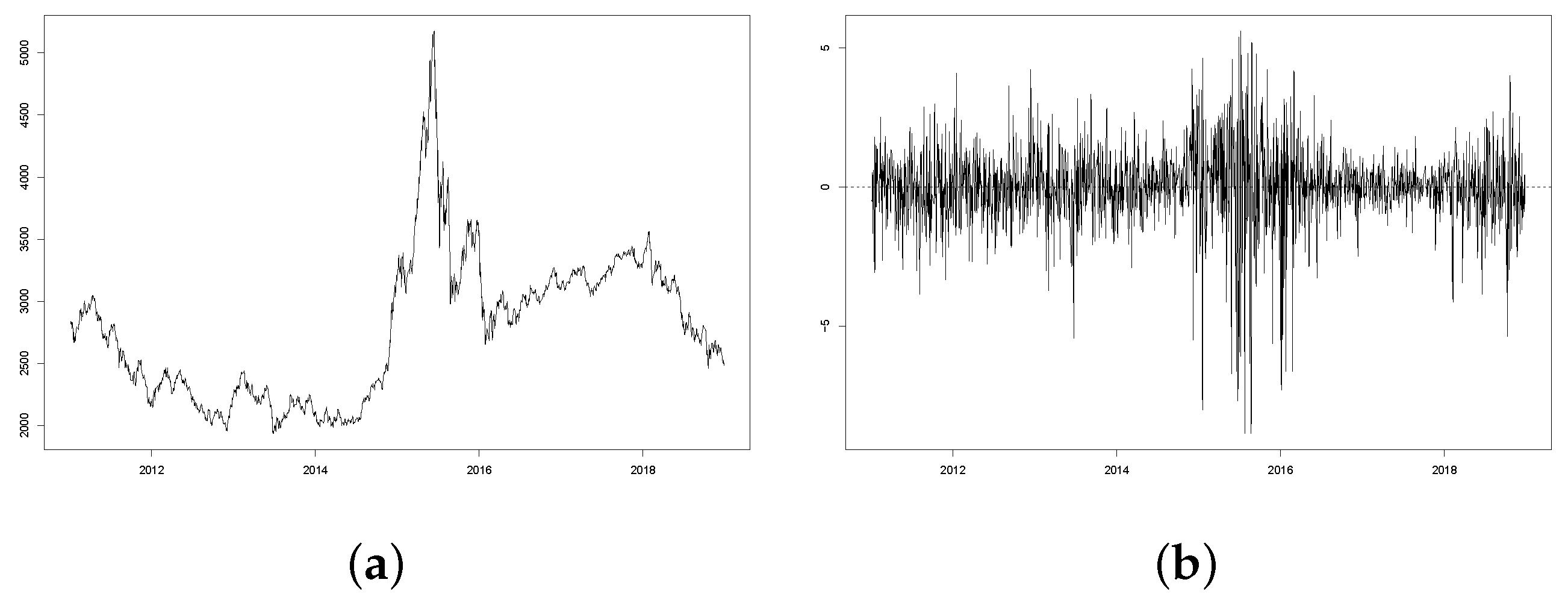
The daily closing prices and returns of SSE are plotted in Figure 1. In the closing price plot, SSEs generally have ranged between 2000 and 3500 over 2011–2018, except for a spike from 2500 to 5000 in early-2015. This spike has led to large variations of return, as observed in Figure 1b. Additionally, most daily returns vary in the [−4%,4%] range, with the largest negative (positive) value below −7% (above 5%) in late-2015. After fitting a standard GARCH(1,1) with Normal assumption, we find that the standardized residuals have a kurtosis of 2.11, suggesting a non-Gaussian distribution. Thus, we perform the Kolmogorov–Smirnov and Jarque–Bera normality tests, where the null hypotheses indicating normality are rejected in both cases (p-values are 0.0000). As a result, CGARCH models with non-Gaussian distributions are expected to outperform the CGARCH-N model.

The estimates of CGARCH(1,1) models with four different distributions are presented in

Table 4. Empirical results: SSE index.

	Normal	t	GED	TS
$\alpha$	0.0546	0.0536	0.0496	0.0483
	(0.0000)	(0.0000)	(0.0000)	(0.0000)
$\beta$	0.9051	0.9441	0.9452	0.8546
	(0.0000)	(0.0000)	(0.0000)	(0.0000)
$\alpha +\beta$	0.9598	0.9977	0.9948	0.9029
	-	-	-	-
$\rho$	0.9982	0.9978	0.9952	0.9983
	(0.0000)	(0.0000)	(0.0000)	(0.0000)
$\varphi$	0.0019	0.0004	0.0004	0.0059
	(0.0388)	(0.1254)	(0.2431)	(0.0013)
$\nu$		4.4566	1.1397
		(0.0000)	(0.0000)
${\alpha }^{+}$				−3.1633
				(0.0000)
${\alpha }^{+}$				0.4105
				(0.0000)
${\lambda }^{+}$				5.4251
				(0.0000)
${\lambda }^{-}$				1.0045
				(0.0000)
p				0.4026
				(0.0000)
Log Lik.	−3024	−2943	−2937	−2920
AIC	6061	5900	5888	5862
BIC	6094	5939	5927	5923

Note: Normal, t, GED and TS are statistics for CGARCH with Normal, Student’s t, GED and tempered stable distribution, respectively. Log Lik. stands for the log-likelihood. The values in the parentheses are the corresponding p-values. AIC and BIC are Akaike and Bayesian Information Criterion, respectively.

. In addition, we also consider the Gaussian copula transformation of the CGARCH-t, the in-sample estimates of which will be identical to those of CGARCH-t without transformation. Overall, estimates of those CGARCH models are close to each other. More specifically, except for $\varphi$, all GARCH parameters are estimated to be significantly different from zero at 5% significance level. Estimated $\beta$ of CGARCH-t (0.9441) and CGARCH-G (0.9452) are slightly greater than those of CGARCH-N (0.9051) and CGARCH-S (0.8546). In contrast, the magnitudes of estimated $\varphi$ of CGARCH-N (0.0019) and CGARCH-S (0.0059) are greater than those of CGARCH-t (0.004) and CGARCH-G (0.0004).

Since the SSE returns are not Normally distributed, we focus on the results of the three fat-tailed CGARCH models. Both transitory and permanent components are quite persistent to their own shocks. Estimated $\alpha +\beta$ are at least 0.90, whereas estimated $\varphi$ are all over 0.99. Hence, we expect that shocks to both $s_t$ and $q_t$ will not quickly die away [2]. As for the impacts of immediate volatility shocks, fitted results suggest the influence on the permanent component is very much close to zero (all smaller than 0.01). Although such influences on transitory component are all estimated to be significant, the magnitudes are limited at around 0.05. To compare the three fat-tailed models, log-likelihood, Akaike Information Criterion (AIC) and Bayesian Information Criterion (BIC) are presented. It can be seen that CGARCH-S is the best performing model based on all criteria. Additionally, CGARCH-G slightly outperforms CGARCH-t, both of which are preferred to CGARCH-N. Hence, the results of the CGARCH-S model are more reliable, which suggest the volatility persistence of the transitory component (0.9029) is around 10% smaller than that of the permanent component (0.9983). In contrast, both CGARCH-t and CGARCH-G suggest those persistences are almost identical and close to one.

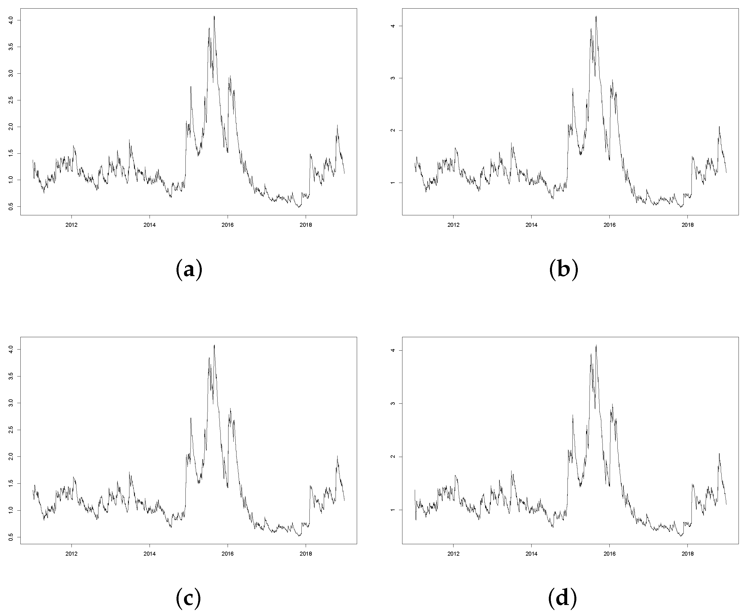
To further explore the models, all the four estimated conditional volatility series (We report conditional volatility here as the square root of $h_t$, so that it has the same scale as $r_t$) are plotted in Figure 2. Despite their different model performances, the four estimated conditional volatility series demonstrate shapes fairly close to each other. Consistent with our previous observations, large variations are found over 2015–2016. Further, due to the impact of large volatility persistences, influences of those shocks do not quickly die away and cause clustering on the conditional volatility.

Despite their similarities, the difference between the fitted conditional volatilities can be described as the different in-sample forecasting performance of the fitted models. To quantitatively compare this performance, we measure the prediction error for each model by $\left|\sqrt{{\widehat{h}}_t}-\left|r_t\right|\right|$, where ${\widehat{h}}_t$ is the fitted $h_t$ for each model, and $|r_t|$ is employed to proxy the true conditional volatility. The results are reported in Panel A of

Table 5. Forecasting performance comparison.

Model	RMSE	Mean	SE	${\mathit{Q}}_{95}$
Panel A: In-sample performance
Normal	1.0245	0.3742	0.9540	1.6078
t	1.0147	0.3540	0.9512	1.5707
GED	1.0140	0.3538	0.9505	1.5639
TS	1.0076	0.3387	0.9492	1.5466
Copula	1.0140	0.3571	0.9533	1.5652
Panel B: Out-of-sample performance
Normal	1.0572	0.8647	0.6145	1.7625
t	1.0433	0.8471	0.6121	1.7222
GED	1.0373	0.8366	0.6163	1.7439
TS	1.0303	0.8293	0.6112	1.7112
Copula	1.0501	0.8519	0.6105	1.7258

Note: SE, RMSE and $Q_{95}$ are standard error, root of mean squared error and 95th percentile, respectively. Normal, t, GED and TS are statistics for CGARCH with Normal, Student’s t, GED and tempered stable distribution, respectively. Copula is the results corresponding to Gaussian-copula transformation of the CGARCH-t model.

. Moreover, to consider the out-of-sample forecasts, we use the last 100 observations as the prediction sample and the others as the training sample. Then, we fit each model for the training sample and calculate the one-step ahead forecast of $h_t$. After that, we include the first observation in the prediction sample and generate another one-step-ahead forecast. We repeat this rolling-window approach until 100 such one-step-ahead forecast $\sqrt{{\widehat{h}}_t}$ are produced. After that, we calculate the absolute difference between them and the corresponding $|r_t|$, which measures the out-of-sample forecasting errors. The results are reported in Panel B of Table 5. It is observed that CGARCH-S leads to the smallest average forecasting errors in both the in-sample and out-of-sample cases. This is confirmed by the RMSE, which is defined as $\sqrt{\frac{1}{100}{\sum }_{h=1}^{100}({\widehat{h}}_{t+h}-|r_{t+h}{\left|\right)}^2}$ and widely used as an overall forecasting performance indicator. Additionally, CGARCH-S produces small variations in the forecasting errors, which is the second smallest for in-sample forecasting and the smallest for out-of-sample forecasting. In addition, when considering $Q_{95}$, the 95th percentile of the forecasting errors, CGARCH-S leads to the smallest extreme errors in both cases. Nevertheless, it is worth mentioning that he copula-transformed CGARCH-t and the original CGARCH-t result in much identical performance. Therefore, this copula model is skipped in the following Value-at-Risk analysis.

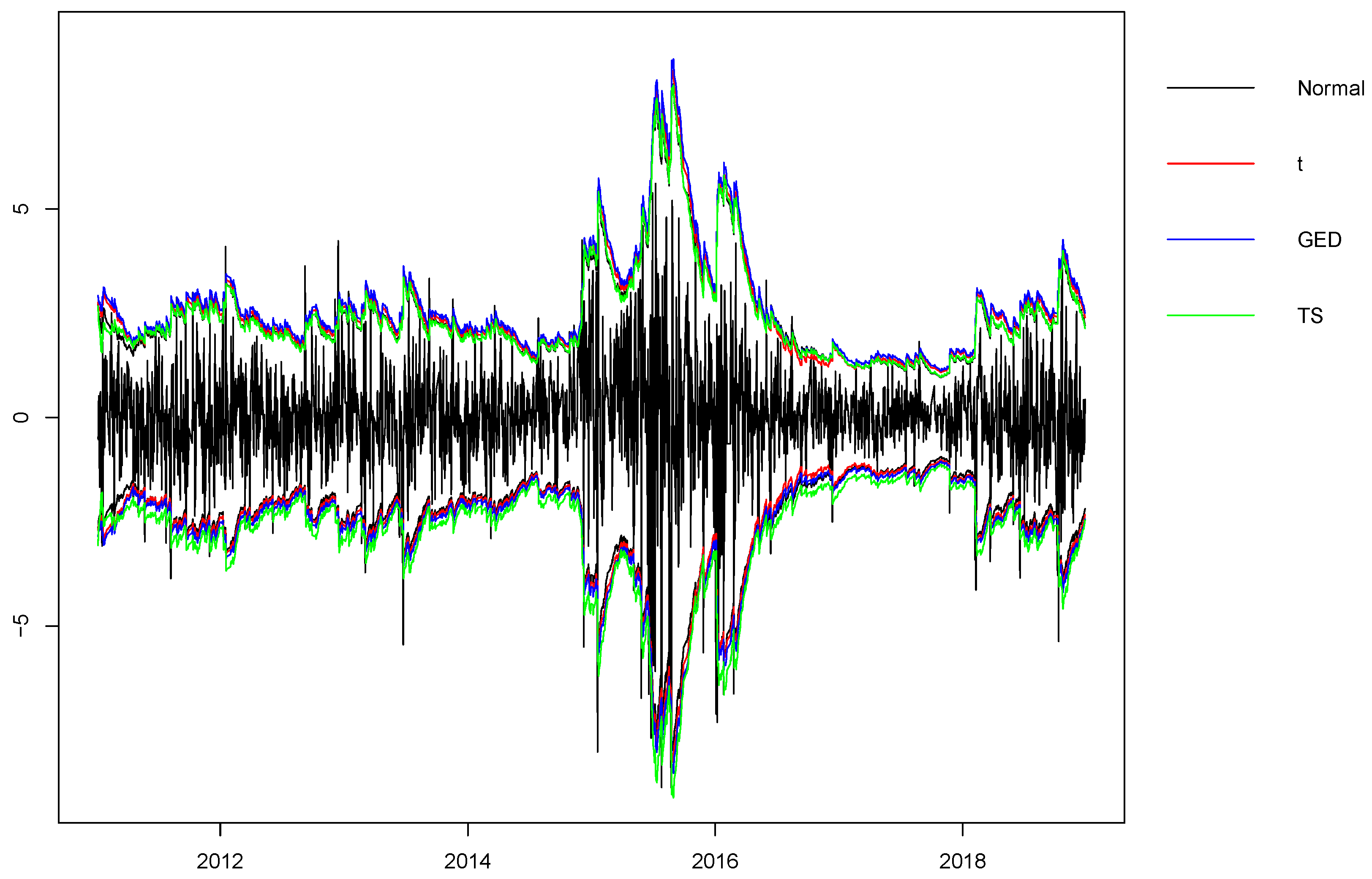
Finally, we consider an important practical application of the CGARCH model: the Value-at-Risk (VaR) analysis. This is particularly useful when measuring the financial risks, such as the investment risk of a portfolio. In this paper, we consider the two-sided 95% VaR, which is constructed as the [$\widehat{\mu }+{\widehat{Q}}_{2.5}\sqrt{{\widehat{h}}_t}$,$\widehat{\mu }+{\widehat{Q}}_{97.5}\sqrt{{\widehat{h}}_t}$], where ${\widehat{Q}}_{2.5}$ and ${\widehat{Q}}_{97.5}$ are the 2.5th and 97.5th percentile of the fitted innovation distribution, respectively. Using the estimated parameters reported in Table 4, it is straightforward to construct the time-varying two-sided 95% VaR for each CGARCH model. The results are plotted in Figure 3. Due to the similarities of $\widehat{h_t}$ as observed in Figure 2, those VaR are again not quite visually distinct from each other. Despite this, it can be seen that both the negative and positive VaR of CGARCH-S are generally smaller than those of the other CGARCH models. Among the total 1944 observations, there are 40 positive ($r_t>$ positive VaR) and 48 negative ($r_t<$ negative VaR) violations for CGARCH-S. Those are quite satisfactory results, standing for 2.1% and 2.5% chances of violation, respectively, which are close to the 2.5% as designed. For the rest, we find 39 positive (2.0%) and 66 negative (3.4%) violations for CGARCH-N, 35 positive (1.8%) and 62 negative (3.2%) violations for CGARCH-t, and 27 positive (1.4%) and 58 negative (3.0%) violations for CGARCH-G. Such results are close to each other and are not as good as those of CGARCH-S. The resulting VaR is clearly biased upwardly for CGARCH-N, CGARCH-t and CGARCH-G models, leading to smaller positive and larger negative violations than expected. The advantage of CGARCH-S on other competing CGARCH models is largely due to the more flexible parametric structure of the tempered stable distributions. In short, the five parameters allow different shapes at each tail and in the middle. Thus, the fitted tempered stable distribution would accommodate more features of the empirical data, such as leptokurtic kurtosis, asymmetric tails and skewness. This leads to more accurate VaR analysis, which is critical for accurate risk-measurement and other risk/portfolio management applications.

6. Concluding Remarks

The CGARCH model has enjoyed particular popularity in finance research for simultaneously studying long- and short-run components. Despite its effectiveness, in practice, the CGARCH model can produce more efficient estimates when appropriate fat-tailed distribution is employed. This paper aimed to find an optimal distribution for disturbances of the CGARCH model, when the underlying distribution was a fat-tailed but unknown type.

Inspired by Calzolari et al. [9], our paper investigated the applicability of the tempered stable distribution within the CGARCH framework. Via systematically designed simulation studies on the CGARCH(1,1) process, we contrasted the performance of CGARCH models with Normal (CGARCH-N), Student’s t (CGARCH-t), GED (CGARCH-G) and tempered stable (CGARCH-S) distributions. The first two studies assumed that the true distributions were the Student’s t and GED, respectively. In such cases, results of CGARCH-S are close to those of the true models, and CGARCH-S uniformly outperforms the other competing models in terms of consistency, efficiency and overall performance. We constructed different combinations of the tempered stable distribution to simulate the CGARCH process in the third study. Our results suggest that none of the CGARCH-N, CGARCH-t and CGARCH-G can perform as well as the CGARCH-S model.

Empirical evidence is further provided to check the robustness of our simulation results in practice. We fit the daily return of the Shanghai Stock Exchange (SSE) index over 2011–2018 into the four CGARCH models, respectively. Our results indicate that CGARCH-S is still preferred to the rest under different model performance criteria, in- and out-of-sample forecasting comparison and Value-at-Risk (VaR) analysis. Nevertheless, the limitations of this research are two-fold. First, we focused on the analysis of SSE index, and more evidence on the feasibility of CGARCH-S model needs to be verified for other financial equities. Second, the current CGARCH framework is limited to a uni-regime model. To cope with empirical structural changes recently caused by major events such as COVID-19, a regime-switching CGARCH model may be proposed and studied. Addressing those limitations sheds light on systematic validation of the practical usefulness of the CGARCH model in areas such as portfolio management and other enterprise risk-management issues.