Comparative Evaluation of Road Vehicle Emissions at Urban Intersections with Detailed Traffic Dynamics

Abstract

The insufficient development of intelligent dynamic monitoring systems, which operate with big data, obstructs the control of traffic-related air pollution in regulated urban road networks. The study introduces mathematical models and presents a practical comparative assessment of pollutant emissions at urban intersections, with two typical modes of vehicle traffic combined, i.e., freely passing an intersection when the green signal appears and uniformly accelerated passing after a full stop at the stop line. Input data on vehicle traffic at regulated intersections were collected using real-time processing of video streams by Faster R-CNN neural network. Calculation models for different traffic flow patterns at a regulated intersection for dynamic monitoring of pollutant emissions were obtained. Statistical analysis showed a good grouping of intersections into single-type clusters and factor reduction of initial variables. Analysis will further allow us to control and minimize traffic-related emissions in urban road networks. A comparative analysis of pollutant emissions in relation to the basic speed of passing at the intersection of 30 km/h was performed according to the calculations of the mathematical models. When reducing the speed to 10 km/h (similar to a traffic jam), the amount of emissions increases 3.6 times over, and when increasing the speed to 50 km/h, the amount of emissions decreases by 2.3 times. Fuzzy logic methods allow us to make a comparative prediction of the amount of emissions when changing both the speed of traffic and the capacity of the intersection lanes. The study reveals the benefits of using a real-life measurement approach and provides the foundation for continuous monitoring and emission forecasting to control urban air quality and reduce congestion in the road network.

1. Introduction

Traffic-related pollutant emissions are the main obstacle to sustainable urban development. In recent decades, they have proportionally increased due to the exponential growth in the road-traffic intensity. Thus, reducing and managing the intensity of traffic-related emissions has become an unprecedented challenge subject to a profound study.

Closed-circuit television cameras are most often used to control and monitor traffic flows. Video cameras can record road traffic offences and obtain initial data on the parameters of the traffic flow used in dynamic monitoring systems, as well as the subsequent regulation of the traffic flows themselves and the environmental status of the urban transport network [1,2].

This study continues the authors’ development of a dynamic system for traffic flow monitoring, which implements real-time control of such parameters as the structure of the vehicle queue and the entire flow, the speed and acceleration of vehicles, and their trajectory at urban, regulated intersections [1,2].

This large volume of initial data is used not only to control and manage traffic flows but also serves as a basis for calculating pollutant emissions using mathematical models based on standard regulatory procedures. An example of such a system is the authors’ AIMS-Eco system: “Intelligent system for real-time monitoring the amount of traffic-related pollutant emissions” [3] based on neural networks.

This paper develops an approach to design a unified urban system for the environmental control of traffic-related pollutant emissions based on the processing of data from video cameras. At the initial stage, we considered only traffic lanes for moving “straight” at intersections as they are most informative in terms of traffic dynamics. We have not considered an isolated, regulated intersection as a source of harmful emissions but identified single-type groups (clusters) of traffic lanes to facilitate managerial decisions aimed at reducing the environmental load on a wider scale. Thus, the purpose of the study is to develop computational mathematical models to implement a system for the dynamic monitoring of pollutant emissions from traffic flows passing a regulated intersection at a variable speed.

A preliminary version of our emission monitoring system has been implemented, examining uniform traffic at successive sections of a 20 m long intersection. To improve the integrity of our system, we must take into account the dynamics of emissions when vehicles accelerate after a stop at a red light. Therefore, to assess the quality of the resulting calculation models, we should complete a comparative prediction of emissions produced when changing the speed of traffic flows.

Section 2 of the paper provides a review of research in this field. Section 3 describes methods for recognizing and classifying, tracking, counting, and determining vehicle speed using neural networks. Section 4 presents a mathematical model of traffic-related pollutant emissions. Section 5 deals with emission forecasting by fuzzy logic methods. Section 6 discusses the obtained results, and Section 7 presents concluding thoughts and further areas of research.

2. Related Works

A report in 2019 indicated that road transport was the principal source of nitrogen oxides (39% of emissions) and a source of coarse particulate matter and fine particulate matter, which affects the health and quality of life of urban residents around the world [4].

The results of the studies carried out by Cheng et al. [5] showed that ultrafine particles, black carbon, and particle-bound polycyclic aromatic hydrocarbons (p-PAHs) mainly resulted from emissions generated by diesel vehicles. The monitoring of heavy metal emissions in the road area showed [6] that high concentrations of Ti, Fe, Cu, and Ba are typical for road sections where heavy vehicles prevail. The proposed model allows one to determine the predominant composition of the fleet on a given road section.

The most popular models for studying traffic-related pollutant emissions in cities are Computer Program to Calculate Emissions from Road Transport (COPERT) [7] and Passenger Car and Heavy Duty Emission Model (PHEM) [8,9].

COPERT emission models (based on the average speed) and PHEM (based on vehicle kinematics) are analyzed and their sensitivity to traffic dynamics is assessed in [10]. The medium-speed approach in free flow conditions tends to overestimate the amount of emissions, while in cases of congestion it tends to underestimate the amount of emissions, ignoring the effects of congestion.

Spyropoulos et al. [11] forecasted vehicle-related emissions using the COPERT method and Brown’s double simple exponential smoothing. When analyzing the data, they found that the measurement results are influenced by such factors as the wind speed and direction, as well as the atmospheric air temperature. To obtain data only on vehicle-related emissions ignoring atmospheric factors, they built a “traffic flow—roadside environment” model. The model assesses air pollution generated only by the traffic flow (TF).

Using an optical remote sensing device to measure the concentrations of CO, CO₂, HC, and NO exhaust gases, ref. [12] calculated average emission factors and compared them with those of the COPERT III model (version 2.1). The authors found that the model overestimated the indicators for almost all technology classes (EURO 1, 2, 3) for CO, and the relationship between the model and measurements was good for HC and NOx emissions, except for heavy vehicles (in the model, the indicators had a lower level compared to the measured data).

Angatha and Mehar [13] studied the influence of the TF parameters, the duration of the red traffic light signal, and the average number of vehicles stopping at the red light on the concentration of carbon monoxide. Two models are proposed: using the methods of multiple linear regression and artificial neural networks. The latter model showed the best results in predicting carbon monoxide values. A linear increase in carbon monoxide with an increase in the number of vehicles at the entrance to the intersection and the duration of the red traffic signal was observed due to changes in the acceleration and deceleration of vehicles at intersections.

The influence of the duration of traffic signals and obeying the TF speed limit on the amount of harmful emissions was considered in [14]. The authors developed a numerical model choosing the optimal traffic light pattern to achieve a balance between delays at regulated intersections for drivers and minimize the amount of harmful emissions. The authors of [15] also analyzed the quality of urban air at a speed limit of up to 80 km/h and found that CO, NOx, and PM2.5 were reduced by 5–7%.

Traffic-related harmful emissions depend on the properties of the vehicles themselves, the type of urban development, geography, and meteorological conditions, which complicate the control and forecasting of the dispersion of harmful substances [16].

All these factors set high requirements for the computational performance of the developed real-time high-accuracy models. The system for vehicle emissions on an urban road network (RTVEMVS) developed in [16] gives a precise real-time assessment of emissions (taking into account the dispersion model) and visualizes the obtained data on a map of the road network. Similar studies and developments were carried out in [17,18,19,20,21].

In an urban environment, harmful substances are dispersed under the influence of the depth of street canyons and air movement caused by moving vehicles [22,23]. Simulation at various wind and vehicle speeds show that moving vehicles strongly influence wind turbulence, which is a significant factor for the dispersion of harmful emissions. Turbulence and air flows generated by vehicles reach a height of 7 to 12 m in the street canyon [24]. Regulated intersections are characterized by the stop and starting of vehicles, as well as the braking mode, which is when high concentrations of harmful emissions are released. The wind ventilation of intersections differs from a common street canyon due to different wind directions [25].

The Euler–Lagrange method was used as the basis of the model for predicting the concentration of harmful emissions and the dissipation rate to study regulated intersections in [25]. The minimum concentrations of harmful emissions are observed when the vehicle movement slows down, while the peak values are observed when the movement starts from the intersection. The authors also found that the distance between traffic lights affects the concentration of PM₁₀. Researchers in [20] demonstrated in a microsimulation environment that the air quality can be improved by the effective management of traffic flows at regulated intersections.

The literature review has shown that most studies consider individual sections of urban road networks to develop models for calculating concentrations and dispersion of harmful emissions. Computer simulation is based on the data on the average speed of traffic flows (according to COPERT), while traffic flows are characterized by various types of movement, especially in urban areas.

To develop a mathematical model based on fuzzy logic methods to calculate traffic-related harmful emissions taking into account the identified features of traffic flows in urban conditions, we focused on the grouping of vehicle traffic lanes and developed a model for two types of traffic flow movements at regulated intersections: uniformly accelerated and uniform movement [26,27].

The novelty of the study is the development of a model in the problem of high-quality and complete collection of data on the amount of traffic-related emissions based on the use of neural network algorithms and fuzzy logic algorithms integrally taking into account the impact of many unpredictable factors, in view of the design features of the road network.

3. Materials and Methods

The methods include the selection of variables used to collect the initial data, data collection, statistical methods for processing the collected information, interpreting the obtained results on the assessment of pollutant emissions, and emission forecasting using fuzzy logic methods. The basic traffic flow monitoring system used to collect initial data should be considered separately.

To achieve our research goal, we needed to develop a system to assess the dynamic parameters of vehicles, such as acceleration and speed. To this end, we divided the task into four subtasks: object detection and classification; object tracking; object counting; and determining the vehicle speed. Figure 1 shows an algorithm for obtaining the data on vehicle accelerations and average speeds.

The first module processes the incoming video stream and receives object predictions using Faster Region-based Convolutional Neural Network (R-CNN) [28]. When obtaining bounding boxes to find the average speed and determine the direction of movement, the objects should be identified by comparing them with the data of previous frames. To train the neural network, we collected a dataset from street surveillance cameras in Chelyabinsk (Russia). We chose the Simple Online and Realtime Tracking (SORT) tracker for vehicle tracking because of its excellent compromise between speed and accuracy [29].

We used the design of the Faster R-CNN architecture [28,30,31,32] to detect and track the trajectory of objects. According to The Microsoft Common Objects in Context (COCO) [33] and Cityscapes [34], this architecture is a benchmark in datasets when many objects are tracked. We used a high-performance SORT tracker to track the trajectory of vehicles [35,36].

We used free-access outdoor video surveillance cameras to collect the data flow [37]. This solution is very easy since it avoids additional installation and co-ordination costs, though difficulties arose in other aspects: a large viewing angle, a high level of occlusion, visibility and number of objects, and various scales.

The screen co-ordinates of objects are converted to geographic co-ordinates using the perspective transformation matrix. To this end, we select four reference points on the camera image and the corresponding four points on the map. The obtained geographic co-ordinates (latitude and longitude) of one object in the current and previous frame, as well as the time between the frames, are used to determine the distance covered. The speed of the object can be calculated using this distance and the time between the frames. Since the neural network determines objects with an error, we selected frames with a difference of one second instead of two consecutive frames for a more accurate determination of the speed and the distance covered. If the obtained speed is less than 2 m/s, the object is considered to be not moving. Such a nonzero speed was taken due to an error in determining the object by the neural network in the frame sequence. The time between the frames where the object did not move is summed up and taken into account to calculate pollutant emissions. Figure 2 shows the binding of the screen co-ordinates to different categories of vehicles.

3.1. Selection of Variables

We collected data at several major urban intersections in Chelyabinsk, Russia. At the initial research stage, we selected lanes corresponding to the movement of vehicles only in a straight line for several large intersections. We recorded both the geometric parameters of these traffic lanes and the entire structure of the intersections. We selected 23 lanes from 10 major urban intersections. The data were collected for passenger vehicles, and we made 10 measurements both for freely passing an intersection and movement after a full stop at a stop line when the red signal appears. In total, we made 460 measurements for several initial variables characterizing the dynamics of passing an intersection. 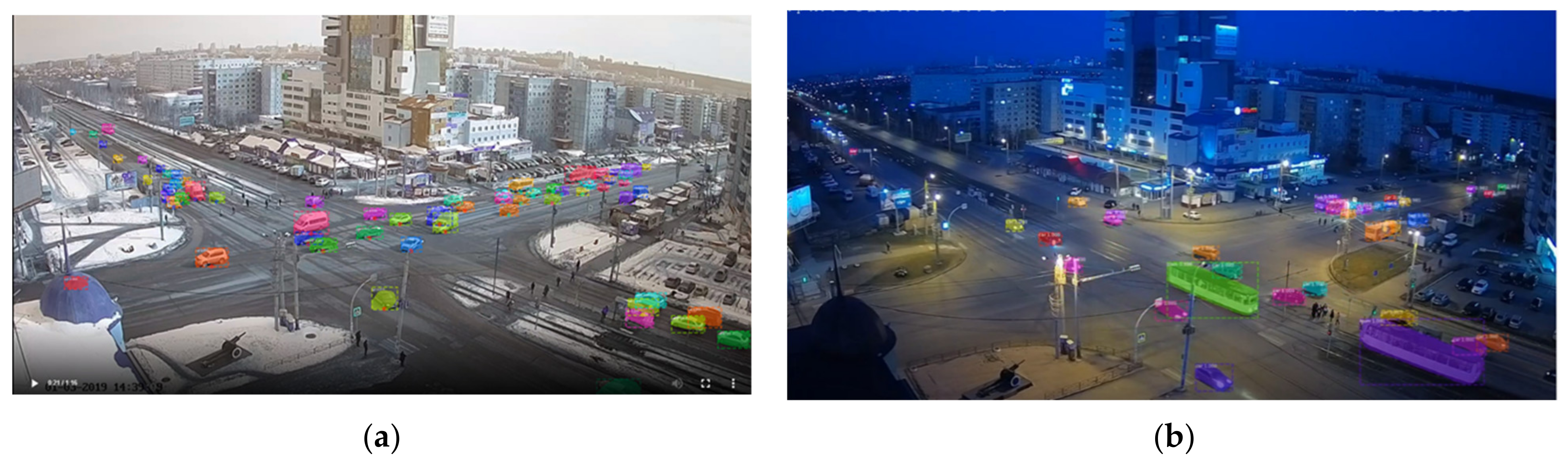Figure 3 shows examples of frames from street cameras for various-geometry intersections crossed by traffic flows.

Table 1. Initial and calculation variables.

No.	Initial and Calculation Variables	Unit of Measurement
	Initial variables
1	L1—distance from the stop line to the 1st conflict point	m
2	L2—distance from the first to the 2nd conflict point	m
3	t1sv—traffic time from the stop line to the 1st conflict point, with freely passing the intersection	s
4	t2sv—traffic time from the 1st to the 2nd conflict point, with freely passing the intersection	s
5	t1ost—accelerated traffic time from the stop line to the 1st conflict point, after a full stop	s
6	t2ost—accelerated traffic time from the 1st to the 2nd conflict point, after a full stop	s
	Calculation variables
7	V1sv—traffic speed from the stop line to the 1st conflict point, with freely passing the intersection	km/h
8	V2sv—traffic speed from the 1st to the 2nd conflict point, with freely passing the intersection	km/h
9	VSRsv—average traffic speed at the intersection, with freely passing the intersection	km/h
10	a1ost—vehicle acceleration from the stop line to the 1st conflict point, after a full stop	m/s2
11	a2ost—vehicle acceleration from the 1st to the 2nd conflict point, after a full stop	m/s2
12	aSRost—average vehicle acceleration at the intersection, after a full stop	m/s2
13	V1ost—traffic speed at the 1st conflict point, when moving after a full stop	km/h
14	V2ost—traffic speed at the 2nd conflict point, when moving after a full stop	km/h
15	VSRost—average traffic speed at the exit from the intersection, when moving after a full stop	km/h
16	Sij—saturation flow of the i-th lane during the j-th regulation phase	equivalent units/h
17	Cij—capacity of the i-th lane during the j-th regulation phase	equivalent units/h

presents the set of initial variables obtained from the video stream used as primary variables in the study, as well as several secondary calculation variables.

The following assumptions were used to calculate the variables S_ij and C_ij. The capacity of the traffic lane at regulated intersections according to [38] is determined by the formula:

$$C_{ij}=\frac{S_{ij}\cdot g_{ej}}{c},$$

(1)

where C_ij is the capacity of the lane i during the regulation phase j, equivalent units/h; S_ij is the saturation flow of the lane i during the regulation phase j, equivalent units/h; g_ej is the effective duration of the regulation phase j, s; C is the duration of the regulation cycle, s.

$$S_{ij}=S_0\cdot N\cdot f_W\cdot f_{HV}\cdot f_G\cdot f_P\cdot f_{BB}\cdot f_A\cdot f_{RT}\cdot f_{LT},$$

(2)

where S₀ is the ideal saturation flow taken equal to 1800 (equivalent units/h); N is the number of traffic lanes; f_W is the coefficient taking into account the width of the traffic lane; f_HV is the coefficient taking into account heavy goods vehicles; f_G is the coefficient taking into account gradients; f_P is the coefficient taking into account parking; f_BB is the coefficient taking into account the interference created by buses; f_A is the coefficient taking into account the area type; f_RT is the coefficient taking into account right turns (i.e., interference created by passengers); f_LT is the coefficient taking into account left turns.

3.2. Statistical Processing of Initial Data

Dividing vehicle traffic lanes into single-type clusters will further allow us to carry out a comparative analysis of pollutant emissions at regulated intersections for these single-type groups, as well as formulate statistically reliable conclusions about the environmental situation in the entire urban transport network for single-type groups of intersections.

Statistical data processing involves the use of the following processing algorithms: clustering; identification of the initial data, which significantly differentiate clusters; and factor analysis to determine factor-grouping trends. The calculations were made in the Statistical Package for the Social Sciences (SPSS) professional statistical suite

3.2.1. Clustering

The initial data space is limited during clustering by the main variables, which determine the design parameters of traffic lanes at intersections, as well as the nature of the actual vehicle movement. These are S_ij—the saturation flow of the lane; L₁ and L₂—the geometry of the intersection; t_1ost and t_2ost—the time of the vehicles’ crossing an intersection after a full stop at the stop line. Notably, the time of freely passing an intersection t_1sv and t_2sv strongly correlates with the variables L₁ and L₂ and is not decisive in our further analysis.

The single type of the selected groups of lanes is determined by the measure of proximity or difference between the values of their characterizing factors according to the square of the normalized Euclidean distance. To determine the distance between clusters, we chose Ward’s method [39,40] as the most correct approach forming “spherical” clusters.

The clustering procedure forms a representation of the sequential combination of initial objects into single-type groups—a dendrogram, indicating the agglomeration distance as a measure of clustering stability.

The dendrogram (Figure 4) clearly shows that the upper group of traffic lanes (12,13,5,6,11,15), distinguished by their length of the lane in the intersection, is allocated into a separate cluster. The two lower clusters of traffic lanes have approximately the same length in the intersection but differ in the ratio of the variables L₁ and L₂, which leads to them being considered to be separate groups. It is no longer essential to divide traffic lanes into more than three clusters stable within the 18% difference scale range.

3.2.2. Comparison of Clusters

Let us determine the importance of variables in the division of the studied traffic lanes into three selected clusters. The answer is given in the procedure for determining the statistical significance α_fact of the influence of each variable according to Fisher’s criterion—based on the assessment of differences in their average values for all the three cluster groups. The calculation results are presented in

Table 2. Differences in the average values of variables for three clusters.

Clusters	Variables (Average Values in Clusters)
	Sij	L1	L2	t1	t2
1 (8 lanes)	1755	20.6	13.8	3.73	1.36
2 (9 lanes)	1649	16.7	19.8	3.41	1.95
3 (6 lanes)	1557	22.3	27.5	3.98	2.47
αfact	0.1%	8.7%	0.0%	11.2%	0.0%

. Taking into account that at α_fact < 5% we confirm the statistical significance of the variable in clustering the initial objects, only the length and time of the initial acceleration of vehicles L₁ and t_1ost are not determinant in clustering, which coincides well with our a priori assumptions—the starting movement of vehicles does not depend on the geometry of the intersection.

3.2.3. Factor Analysis

We use the method of multidimensional scaling (factor analysis) to assess the relationship of the set of analyzed variables. This method establishes a relatively narrow set of “properties” for a set of initial and calculated variables. These properties characterize the relationship between groups of these variables and the named factors, which allows us to group the initial variables themselves.

There are various methods of factor analysis. In this study, we use the generally accepted approach of principal component analysis. We rotate factors to obtain a simple structure of interpreting the selected factors, which corresponds to a large load of each variable for only one factor and a small load for all other factors (

Table 3. Rotated component matrix.

Initial Variables	Component
	1	2	3	4
Sij	−0.919
L2	0.897
Cij	−0.876
t2sv	0.804
t2ost	0.769
t1ost		0.913
L1		0.871
t1sv		0.807
a2ost			−0.958
a1ost			0.718
V1sv			0.697
V2sv				0.955

). We use the Varimax orthogonal method [41], which is the most popular rotation option.

The scree plot shown in Figure 5 demonstrates four new grouping factors. These are four points lying on the steep slope of the scree area. The remaining points with eigenvalues less than one can be considered negligible, lying at the foot of the rocky slope.

According to the factor analysis, the initial 12 variables are reduced to the four new factors, the relationship of which is expected a priori and represented by the following groups:

• Factor 1. Variables (S_ij, C_ij, L₂, t_2sv, t_2ost) characterizing the geometry of the intersection and free movement of vehicles through it;
• Factor 2. Variables (L₁, t_1sv, t_1ost) characterizing the geometry of the intersection and accelerated movement after a full stop;
• Factor 3. Variables (a_1ost, a_2ost, V_1sv) characterizing uniformly accelerated movement after a full stop and free movement before an intersection;
• Factor 4. Variable (V_2sv) characterizing the free movement of vehicles at an intersection.

Findings. The statistical analysis showed the statistical reliability of dividing traffic lanes into three single-type clusters, which differ both in the geometry of an intersection and the corresponding nature of the vehicle movement.

The next part of the study is aimed at assessing the differences in pollutant emissions generated by traffic flows crossing the intersections of the highlighted cluster groups.

4. Mathematical Model of Pollutant Emissions

The dynamic parameters and structure of traffic flows determine the amount of vehicle emissions. A high-resolution analysis of the traffic-related emission inventory has shown that the influence of the flow parameters can significantly reduce the total car emissions [42]. Model solutions for estimating traffic-related emissions are the European Road Transport Emission Inventory Model (COPERT) and the Danish Operational Street Pollution Model (OSPM) [43]. These dispersion models, characterized by different degrees of complexity, can describe dispersion conditions using a small amount of manually collected empirical data and predict the relationship between the amount of emissions and concentration levels on the road network. However, to obtain continuous and objective data, model calculations should be based on real-time emission data, and their estimation is not trivial. Significant uncertainty is still associated with accurate emission data due to the complicated data collection procedure caused by the constantly changing amount and pattern of the traffic flow over time and road network parameters [44].

We used a method for calculating pollutant emissions to eliminate the influence of external factors and obtain only the data on the pollution caused by vehicles riding along roads [45,46]. The existing traffic monitoring system provides information on acceleration and average speed, as well as individual vehicle trajectories and categories. The use of neural network algorithms for a continuous assessment of traffic flows will provide much more dynamic and accurate environmental information than the static models of emission inventory assessment.

According to the approved standards [45,46], emissions from vehicles moving at a variable speed M_LV (g/s) are generally determined by the formula:

$$M_{LV}={\displaystyle \underset{0}{\overset{t_1}{\int }}\left(\frac{L_0}{1200}\cdot {\displaystyle \sum _1^k{M}_{k,i}^L}\cdot G_k\right)}\cdot r_V\left(t\right)dt=C_0\cdot {\displaystyle \underset{0}{\overset{t_1}{\int }}{r}_V\left[V\left(t\right)\right]dt},$$

(3)

where: L₀ is length of the road section, km; $M_{k,i}^L$ is specific mileage emission of the i-th pollutant of the k-th type of vehicle, g/km; G_k is the intensity of the traffic flow of each of the k-groups of a certain section of the road per unit of time in all lanes; k is number of vehicle groups; r_V [V(t)] is a correction factor determined by the current speed of the traffic flow V(t); t₁ is the time needed to the traffic flow to cross the intersection of the length L₀; C₀ is a constant characterizing the structure and intensity of the traffic flow (4):

$$C_0=\frac{L_0}{1200}\cdot {\displaystyle \sum _1^k{M}_{k,i}^L}\cdot G_k.$$

(4)

Regulatory documents contain only tabulated values for the factor r_V [V(t)] depending on the speed of the traffic flow (

Table 4. Correction factor r_V [V(t)].

Vi	rV [V(t)]
5	1.4
10	1.35
15	1.3
20	1.2
25	1.1
30	1
35	0.9
40	0.75
45	0.6
50	0.5
60	0.3

).

However, computer calculations provide for its analytical dependence obtained by approximation for the permissible range of urban traffic speeds up to 60 km/h. The analytical expression of the trend was obtained using the simplest equation with the maximum approximation confidence level of 99.9%, which will be used in our comparative assessments of pollutant emissions:

$$r_V\left[V\left(t\right)\right]=b_3\cdot V{\left(t\right)}^3-b_2\cdot V{\left(t\right)}^2+b_1\cdot V\left(t\right)+b_0.$$

(5)

According to (3) and (4), the equations determine the computational mathematical model for a computer system of monitoring pollutant emissions from a traffic flow moving at an arbitrary speed. However, it is very difficult to use it in practice due to the need to calculate the instantaneous speeds of the entire traffic flow.

For the practical applicability of the computational model, we further considered two variants of the traffic flow movement within an intersection according to the initial data array—uniform movement and uniformly accelerated movement after a full stop. This corresponds to freely passing an intersection without stopping and accelerated movement after a full stop at a red light.

4.1. Uniform Movement

For the constant speed of the traffic flow V₀, Equation (3) is simply written as follows:

$$M_{LV}=C_0\cdot r_{V0}\cdot t_1,$$

(6)

where r_V0 is the correction factor determined (from Table 4) at the known speed V₀; t₁ = (L₀/V₀) is the time needed for the traffic flow to pass an intersection with the length L₀.

Let us compare emissions at the intersection length L₀ from a flow of vehicles moving at a constant speed V₀ for different levels of speed V₀. Let us assume that the base value of pollutant emissions is expressed by the emissions from the traffic flow at r_V0 equal to one, which corresponds to a speed V₀ = 30 km/h.

Then, the comparative emission factor at an arbitrary constant speed of the traffic flow and a base speed of 30 km/h (K_Vi/30) is determined, taking into account analytical dependence (5), according to the formula:

$$K_{Vi/30}=\frac{C\cdot r_{Vi}\cdot t_i}{C\cdot r_{30}\cdot t_{30}}=\frac{30}{r_{30}\cdot V_i}\cdot r_{Vi}=\frac{C_1}{V_i}\cdot \left(b_3\cdot V{\left(t\right)}^3-b_2\cdot V{\left(t\right)}^2+b_1\cdot V\left(t\right)+b_0\right).$$

(7)

The comparison factor K_Vi/30 is shown graphically in Figure 6.

According to the calculations, the amount of pollutant emissions strongly depends on the average speed of the traffic flow. So, with a decrease in the average speed from 30 km/h to 10 km/h, the amount of emissions at the intersection is four times larger. With an increase in the average speed from 30 km/h to 50 km/h, the amount of emissions at the intersection is three times smaller. This analysis shows the extent to which emissions are reduced by increasing the average vehicle speed.

4.2. Uniformly Accelerated Movement

Let us compare the degree of the increase in pollutant emissions caused by vehicles moving with a uniform acceleration after a stop at the red signal and reaching the speed V₀ after leaving the intersection, in relation to the uniform movement at the speed V₀.

In this problem statement, the relative emission comparison factor for a uniformly accelerated and uniform movement of the traffic flow at the speed V₀ is calculated as follows:

$$K_{V0}=\frac{M_{L{V}_0}^{\prime }}{M_{L{V}_0}^{″}}=\frac{{\displaystyle \underset{0}{\overset{t_1}{\int }}\left(b_3\cdot {\left(a_{0}t\right)}^3-b_2\cdot {\left(a_{0}t\right)}^2+b_1\cdot \left(a_{0}t\right)+b_0\right)dt}}{r_{V_0}\cdot t_2},$$

(8)

where t₁ is the time of the vehicle acceleration from 0 to V₀; a₀ = V₀/t₁ is the constant vehicle acceleration; t₂ = L₀/V₀ is the time of the uniform movement of vehicles on the same section L₀, at t₂ = t₁/2.

Figure 7 graphically represents the comparison factor K_Vi at various final acceleration rates V₀.

According to the calculations, the increase in emissions varies from at least two times at low speeds, and up to six times at a speed of 60 km/h. This confirms the environmental expedience of enabling vehicles to move through intersections without stopping.

4.3. Total Emissions at Intersections

Assuming that the shares of vehicles passing the intersection without stops and after a full stop at the stop line are equal, we can sum the emissions by the comparison factors K_Vi/30 and K_V0 in terms of V₀ of 30 km/h–K_V0/30 (Equations (7) and (8)). The total numerical measures (K_sm) (Equation (9)) of comparison in relation to the speed V₀ = 30 km/h are presented in

Table 5. The ratio of pollutant emissions at the intersection at different speeds of the traffic flow.

Vi	KVi/30	Ksm
10	4.05	12.31
15	2.60	8.01
20	1.80	5.74
25	1.32	4.37
30	1	3.45
35	0.77	2.79
40	0.56	2.24
45	0.40	1.82
50	0.30	1.51
55	0.23	1.33
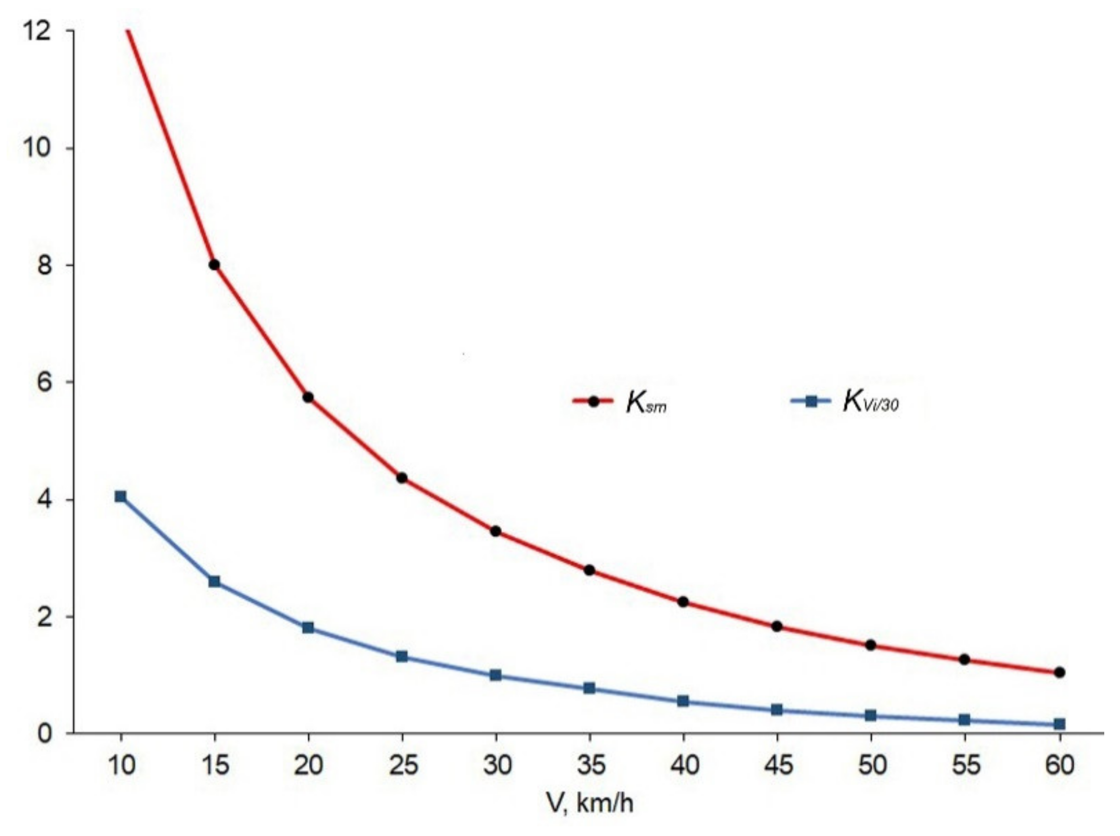
60	0.15	1.05

, and the graphical representation of K_sm on the background of K_Vi/30 is shown in Figure 8.

$$K_{sm}=K_{Vi/30}+K_{V0/30},$$

(9)

According to the comparison of the total emissions at the intersection in relation to the free movement of a traffic flow at a speed of 30 km/h, when the vehicle speed increases, the total emissions change significantly. So, when decreasing the speed of the traffic flow to 10 km/h (similar to a traffic jam), the amount of emissions increases by 3.6 times, and when increasing the speed to 50 km/h, the amount of emissions decreases by 2.3 times.

To create a practical calculation model of pollutant emissions, we should determine the structure and intensity of the traffic flow (this calculation has already been implemented in a working system) and calculate emissions at a speed of 30 km/h. Next, we determine the acceleration of vehicles after a stop at the stop line and their speed at the exit from the intersection. Based on Equations (6)–(8), we determine the total traffic-related emissions at the intersection. These tasks can be easily implemented in practice to instantaneously calculate vehicle speed when the traffic flow crosses the entire intersection.

4.4. Comparison of Clusters by Pollutant Emissions

Let us compare three cluster groups of intersections in terms of several traffic flow characteristics, which are practically significant for assessing pollutant emissions.

Table 6. Differences in the average values of variables for the three clusters.

Clusters	L1	L2	aSRost	VSRost	VSRsv	Sij	Cij
1 (8 lanes)	20.63	13.75	2.65	48.73	52.32	838.0	1755.0
2 (9 lanes)	16.67	19.78	2.53	49.77	48.23	694.3	1648.8
3 (6 lanes)	22.33	27.50	2.40	58.07	50.02	493.2	1557.0
αfact, %			53.8	0.6	43.1	0.3	0.0

presents the data and their level of statistical significance (α_fact) of differences for the three clusters as determined by Fisher’s criterion in the SPSS suite.

A statistically significant difference between the cluster groups of intersections is determined by the speed of the vehicles leaving the intersections V_SRost, as well as the saturation flows S_ij and the traffic lane capacity C_ij.

Let us differentiate between the three clusters of intersections in terms of the total emissions taking into account the calculations shown in Figure 5 with the determinant factor V_SRost. If we take the total emissions for the first cluster as 100%, the emissions for the second cluster will be 96.9%, and for the third cluster—72.5%. According to the Chi-square statistical test, the level of statistical significance of differences in the total emissions is negligible (asympt.value = 0.000), which indicates a high level of statistical significance in differences in the total emissions for the selected clusters of intersections. The calculation results are presented in

Table 7. Differences by pollutant emission clusters.

Total Emissions				Test Statistics
Clusters	Observed Emissions, %	Expected Emissions, %	Balance		Total Emissions
1	100.0	898.0	102.0	Chi-square	50.528
2	96.9	898.0	71.0	Degree of freedom	2
3	72.5	898.0	−173.0	Asympt. Value αfact	0.000
Total	269.4

.

5. Emission Forecasting by Fuzzy Logic Methods

The considered algorithm for calculating the amount of traffic-related pollutant emissions does not take into account many unpredictable, random factors, such as a sharp change in weather conditions, nonperiodic traffic jams, accidents, unpredictable interference, etc. In this case, it is expedient to use situation forecasting methods based on fuzzy logic algorithms, which integrally take into account the impact of many unpredictable factors. Taking into account the impact of such random factors separately is very difficult because of the complexity of obtaining initial data to analyze their impact.

To visualize the influence of fuzzy factors on pollutant emissions at a regulated intersection, we construct a general model using the fuzzyTECH8.77e computer program to assess the influence of the vehicle speeds when freely passing the intersection V_SRsv and a uniformly accelerated movement after a full stop V_SRost, as well as the reduced capacity of the traffic lane C_ij, on total pollutant emissions (SumVBR).

The initial set of the observation data on 23 traffic lanes at urban intersections was used as a basis. The simulation was based on the Gaussian nature of the membership functions since it reflects the best of the unpredictability of many influencing factors, which are difficult to take into account. The levels of membership functions are determined disproportionately because of the nonlinear nature of the dependence of emissions on the vehicle speed.

Figure 9 shows the block diagram of the constructed model, as well as Gaussian membership functions of V_SRost (V_SRsv similarly) and C_ij and the output variable SumVBR. Gaussian fuzzification is most consistent with the stochastic version of the problem. The parameters of the Gaussian terms were determined according to the authors’ expert estimates based on their practical work with surveillance camera data.

The block of correspondence rules with three level input variables consisting of 27 rules is too bulky, and it also formed according to the expert estimates based on the practical work with traffic flows.

The experimental studies of the constructed model predict the output variable based on the actual values of the input variables, as well as graphically represent the distribution field of their mutual influence in the form of volumetric surfaces. Thus, Figure 10 shows the dynamics of the total pollutant emissions (on a relative scale) at a variation in lane capacity of 25%, 50%, and 75% of the maximum value of 1200 equivalent units of vehicles per hour.

The simulation results demonstrate a similar influence of the speeds of traffic flows V_SRsv and V_SRost on the total emissions, as well as the determinant nature of the influence of the traffic lane capacity of the intersection. This study can serve as a useful basis for making reasoned decisions to reduce pollutant emissions using regulated intersection control.

6. Discussion

There are two types of movement of traffic flows at regulated traffic lights in an urban network: moving through the intersection without stopping and accelerated movement after a full stop at a red light.

Analysis of the initial data on the vehicle movement along 23 lanes allowed us to group the lanes into single-type clusters that differ with a statistical significance both in the geometry of the intersection and in the nature of the vehicle movement along them. The factor analysis of the initial data array also showed single-type groups of initial parameters distinguishing these traffic lanes. Statistically reliable clustering of the traffic lanes allowed us to give a comparative assessment of the environmental situation in the urban transport network nodes based on the obtained, practically applicable mathematical model.

We presented a complete mathematical model for calculating pollutant emissions, although it is difficult to apply it in practice. We proposed to simplify it to a working version by considering the above two characteristic types of the traffic flow movement at urban intersections. The approbation of such a practically applicable calculation model is demonstrated in the form of a comparative analysis of all emissions at the intersection in relation to the speed of the traffic flow of 30 km/h. Therefore, when reducing the speed of the traffic flow to 10 km/h (similar to a traffic jam), the amount of emissions increases by 3.6 times, and when increasing the speed to 50 km/h, the amount of emissions decreases by 2.3 times.

We presented a generalized forecast for pollutant emissions at regulated intersections using fuzzy logic. The simulation results demonstrate the similar influence of the speeds of two types of traffic movement on total emissions, as well as the determinant nature of the influence of the traffic lane capacity at intersections.

The detection of a statistically significant difference in traffic-related pollutant emissions when changing the speed at intersections can assist in making sound management decisions to minimize pollution in the urban transport network.

7. Conclusions

We proposed and tested a method to identify single-type groups of traffic lanes at urban intersections, which will allow for the minimization of a number of standard management decisions to reduce traffic-related pollutant emissions. We have developed a complete mathematical model which calculates emissions while taking into account the arbitrary speed of traffic flows as well as a simplified calculation model based on identifying the two typical modes of vehicle traffic at intersections: moving through the intersection at a constant speed (without stopping) and uniformly accelerated movement after a full stop at a red light. When using the simplified model, the calculated load on the dynamic monitoring system becomes acceptable, providing for stable, real-time operation. This approach is closer to reality than the calculation models used in the AIMS-Eco system.

When implementing the proposed simplified calculation model to determine emissions in the AIMS-Eco system, we expect a high approximation of the calculation results to the instrumental test measurements of emissions made by public environmental monitoring centers.

Further studies will focus on all the traffic lanes in a regulated intersection in order to assess the overall environmental situation at intersections and minimize emissions. This study can also serve as a basis for a simplified design of a system for environmental monitoring in the urban transport network based on the clustering of many urban intersections.