Article

Optimal Timing Fault Tolerant Control for Switched Stochastic Systems with Switched Drift Fault

1
School of Mathematics Science, Liaocheng University, Liaocheng 252000, China
2
Key Laboratory of Measurement and Control of CSE Ministry of Education, School of Automation, Southeast University, Nanjing 210096, China
3
New Drug Research and Development Co., Ltd., State Key Laboratory of Antibody Research & Development, NCPC, Shijiazhuang 052165, China
*
Authors to whom correspondence should be addressed.
Mathematics 2022, 10(11), 1880; https://doi.org/10.3390/math10111880
Submission received: 31 March 2022 / Revised: 22 May 2022 / Accepted: 27 May 2022 / Published: 30 May 2022

Abstract

:
In this article, an optimal timing fault tolerant control strategy is addressed for switched stochastic systems with unknown drift fault for each switching point. The proposed controllers in existing optimal timing control schemes are not directly aimed at the switched drift fault system, which affects the optimal control performance. A cost functional with system state information and fault variable is constructed. By solving the optimal switching time criterion, the switched stochastic system can accommodate switching drift fault. The variational technique is presented for the proposed cost function in deriving the gradient formula. Then, the optimal fault tolerant switching time is calculated by combining the Armijo step-size gradient descent algorithm. Finally, the effectiveness of the proposed controller design scheme is proved by the safe trajectory planning for a four wheel drive mobile robot and numerical example.

1. Introduction

The switched system is a complex kind of hybrid system, which consists of a family of subsystems and a switch rule that coordinates the sequence of the subsystems. The switch rule is triggered by switching signals [1,2]. Compared with nonswitching systems, switching systems have higher control flexibility. Switched systems with unstable subsystems can be stabilized by designing reasonable switching rules [3,4]. Switched control systems have been given considerable attention, not only to the inherent complexity, but also the wide range of practical applications. There are numerous industrial control processes that could be modeled as the switched systems, such as wind energy conversion [5], chemical reactors [6], hybrid electric vehicles [7], robot motion planning [8], etc.
For switched systems, the optimal control problems have attracted wide attention from researchers [9,10,11]. Different from the traditional continuous systems, the objective of switched system optimal control is to calculate the optimal switching sequence and switching rules to optimize the cost function, see [12] for a recent survey. After years of development, the optimal timing control of continuous systems has made great progress [13,14,15,16]. However, these conclusions may be infeasible when the systems are complex switched systems. For a class of autonomous systems in which the sequence of continuous dynamics is predefined, the authors of [17] proposed the optimal time switching strategy by computing the cost function and the gradient over an underlying time grid. Considering the relatively simple cost functional, the study described in [18] combined with a gradient descent algorithm gives the gradient formula for the switching time. The previous results mostly focus on the cost function containing only integral terms. Although the cost functional in [17] is relatively more general, it cannot meet the needs of some special working conditions, such as flexible satellite attitude optimization [19] or multi-agent vehicle formation planning [20]. It is necessary to study the time optimal switching problem of the generalized cost functional with the integral term and terminal term.
Since disturbance terms often exist in practical systems, it is almost impossible to construct an accurate mathematical model to describe practical switched systems [21,22,23]. At the same time, the stochastic disturbances lead to the stochastic characteristic of switched systems. From a practical application point of view, stochastic switched systems can model complex dynamics, uncertainty, randomness. Considering the inevitable effect of noise and stochastic disturbance, the authors of [24] investigated the time optimal switching strategy for linear stochastic switched systems. The optimal control strategy for discrete-time bilinear systems is extended to switched linear stochastic systems in [25]. For general multi-switched time-invariant stochastic systems, the authors of [26] proposed the time optimization control approach by minimizing a cost functional with different costs defined on the states. However, it is worth mentioning that the aforementioned schemes are only applicable to systems in good operating conditions (i.e., fault free). Extra efforts are needed to analyze the fault tolerant control problem for switched stochastic systems.
With the increasing demand for safety critical systems in both military and civilian applications, the performance and safety issues need to be specially considered despite the presence of faults [27]. This stimulates the research of a fault tolerant control system that can accommodate unknown system faults and maintain its prespecified performance [28,29,30]. In consideration of the actuator fault, the authors of [31] designed the fault tolerant controller for a class of uncertain switched nonlinear systems. The actuator saturation fault has been investigated for a class of discrete-time switched systems [32]. For the switching point perturbation, the robust optimal control of switched autonomous systems is derived in [33]. For switched parabolic systems described by partial differential equations, the boundary system fault is researched in [34]. With the above observations, the fault tolerant control for stochastic switched systems has not been well developed yet. It is a common phenomenon that the switching time fault occurs in practical switched engineering systems. The switching signals are easily subject to electromagnetic interference and unknown abrupt phenomena such as component and interconnection failures. These factors can induce the switch time to have a delay [31] and drift faults. In addition, from the optimal control point of view, the cost function may increase rapidly and serious security accidents have occurred during the control process when the switching time exceeds or lags behind the designed optimal switch time. However, as far as we know, there are few results about optimal fault tolerant control for switched stochastic systems with switched drift fault. The challenges outlined above motivate us to focus on the optimal timing fault tolerant control problem for switched stochastic systems.
The remainder of this article is arranged as follows: The problem formulation and the control objective are stated in Section 2. Section 3 presents the main results for signal switching, more switchings and optimal fault tolerant algorithm. Section 4 illustrates the obtained result applications in a four wheel drive mobile robot and numerical example. Section 5 provides some concluding remarks.

2. Problem Formulation

Consider the switched stochastic system depicted as follows:
x ˙ ( t ) = A i x ( t ) + B i ω ( t ) , t [ T i 1 , T i ] , i [ 1 , 2 , , N + 1 ] ,
where x ( t ) n is the state vector, A i and B i are a set of given constant real matrices of appropriate dimensions. T 0 denotes the initial time, T 1 , , T N ( T 0 < T 1 < < T N < T N + 1 = T f ) denote the time switching signal and T f denotes the final time. ω is the stochastic disturbance.
Initial condition x 0 n is a stochastic vector with mean m 0 and variance matrix P 0 ,
E [ x ( t 0 ) ] = m 0 , V a r [ x ( t 0 ) ] = E [ ( x 0 m 0 ) ( x 0 m 0 ) T ] = P 0 .
By employing the property of mathematical expectation for the stochastic initial vector, we have the mean vector m 0 n and variance matrix P 0 n × n . Since the discretization of the time and dynamic input approaches can bring about computation explosions and result in inaccurate solutions, in this paper we focus on a class of switched autonomous systems. Then, the switching time signals are the system input variables.
For the stochastic disturbance, the following condition is imposed.
Assumption A1.
The stochastic disturbance ω is the zero-mean Gaussian white noise process, which is independent of x ( t 0 ) . The following statistical properties are satisfied:
C o v [ ω ( t ) , ω ( τ ) ] = E [ ω ( t ) ω T ( τ ) ] = Q 0 δ ( t τ ) ,
C o v [ x ( t 0 ) , ω ( τ ) ] = E [ ( x 0 m 0 ) ω T ( τ ) ] = 0 ,
where δ ( t ) is the Dirac delta function,
+ δ ( t ) d t = 1 , δ ( t ) = 0 , t 0 , + , t = 0 .
The normal switching time is denoted as T = ( T 1 , , T N ) . The actuator switched fault is an unpermitted deviation T ϵ of the designed standard switching signal input T. The unknown switched drift fault for each switching point can be described as:
T ϵ = ( T 1 + ϵ 1 , , T i + ϵ i , T N + ϵ N ) ,
where the ϵ i is unknown drift parameters.
Assumption A2.
The drift fault parameters are limited to the bounded region, δ i ϵ i δ i , where δ i is a given small positive constant. For δ i , T i + δ i T i + 1 , the predefined triggered sequence of subsystems is continuous and there is no jump. In addition, the switched system states are continuous at the switching time which is different from the general hybrid system.
Remark 1.
Assumption 1 is reasonable and commonly used. In fact, for the practical engineering system, the stochastic noise disturbance is generated by the equipment plant, and is independent of the initial state of the system model. An actuator switched drift fault is a common type of fault. The drift fault parameter ϵ i is brought by electromagnetic interference, transmission delay, equipment aging and mechanical wear in modern engineering applications. It is meaningful and reasonable to limit the amplitude of the drift fault parameter ϵ i . The subsystem triggered sequence does not jump. Assumption 2 is the foundation of fault tolerant control switch system research.
Due to the stochastic characteristic of the system state x ( t ) , the nominal cost functional J 0 is described as:
J 0 = E { Ψ ( x ( t f ) ) + i = 0 N T i T i + 1 L i + 1 ( x ( t ) ) d t } ,
where L i + 1 ( x ( t ) ) = 1 2 x T ( t ) Q i x ( t ) are the running cost functions. Ψ ( x ( t f ) ) = 1 2 x T ( t f ) P T x ( t f ) denote the terminal cost term at the final time. The coefficient matrices P T = P T T 0 ,   Q i = Q i T 0 are the weight matrices for the present and terminal states, where P T n × n and Q i n × n .
Motivated by the integral mean value theorem, a novel cost functional mechanism is investigated to achieve an appropriate compromise between drift fault compensation and the optimal process.
J = E { Ψ ( x ( t f ) ) + 1 2 N i = 1 N δ i δ 1 δ 1 δ N δ N [ t 0 T 1 + ϵ 1 L 1 ( x ( t ) ) d t + + T i + ϵ i T i + 1 + ϵ i + 1 L i + 1 ( x ( t ) ) d t + + T N + ϵ N t f L N + 1 ( x ( t ) ) ] d ϵ N d ϵ 1 } .
Remark 2.
It is worth mentioning that the cost function (8) is the mean value of the integral over the switch fault time T ϵ . When the drift fault parameter δ i 0 , ϵ i 0 , i.e., fault free, by utilizing the L’H o ^ pital’s rule, the cost functional (8) becomes the nominal cost functional J 0 . The constructed cost functional J includes system state information and a fault variable, then the optimal switching time obtained by this cost functional is a relatively accommodated switching drift fault.In addition, the proposed cost functional mixes the integral term and terminal term. Therefore, the cost functional (8) we investigate in this paper is general and powerful enough to describe many industrial process.
Control objective: The main purpose of this paper is to deduce the gradient formula for the corresponding cost function with respect to a switched stochastic system (1). Then, under Assumptions 1 and 2, we solve the optimal switching signal criterion, such that the the proposed cost function (8) is minimized in spite of the switched drift fault (6).

3. The Main Results

In this section, we firstly take N = 1 as one switching time for the system. By employing the calculus of variations and some computation, the increment of the cost functional will be deduced according to the switching signal increment. Based on the gradient descent algorithm, the optimal time fault tolerant control of the switched stochastic system is proposed. Then, the multi-switchings time case can be achieved as the single switching time extension. Finally, the optimal fault tolerant algorithm is proposed with a flow chart.

3.1. Single Switching

Consider the case of a single switching for the linear switched autonomous stochastic system with switching time drift fault ϵ ,
x ˙ ( t ) = A 1 x ( t ) + B 1 ω , t [ t 0 , T 1 + ϵ ] , A 2 x ( t ) + B 2 ω , t [ T 1 + ϵ , t f ] .
For the switching time, we take a positive variation Δ t . Compared with the nominal system (9), we denote x ˜ to represent the state trajectory of the system switching time after the increment of Δ t , that is, the switching time is T 1 + ϵ + Δ t . The increment system x ˜ is defined as:
x ˜ ˙ ( t ) = A 1 x ˜ ( t ) + B 1 ω , t [ t 0 , T 1 + ϵ + Δ t ] , A 2 x ˜ ( t ) + B 2 ω , t [ T 1 + ϵ + Δ t , t f ] .
A portion of the grid is presented in Figure 1 to illustrate the different switching times.
In order to make the induced variation cost functional Δ J clear and easy to be represented, one can consider the statistical properties of the stochastic states with the nominal system x and the increment systems x ˜ .
The second-order origin moment matrix of the system states x ( t ) and x ˜ ( t ) satisfy the following matrix differential equation:
m ˙ x ( t ) = A 1 m x ( t ) + m x ( t ) A 1 T + B 1 Q 0 B 1 T , t [ t 0 , T 1 + ϵ ] , A 2 m x ( t ) + m x ( t ) A 2 T + B 2 Q 0 B 2 T , t [ T 1 + ϵ , t f ]
with the initial state m x ( 0 ) = P 0 + m 0 m 0 T .
m ˙ x ˜ ( t ) = A 1 m x ˜ ( t ) + m x ˜ ( t ) A 1 T + B 1 Q 0 B 1 T , t [ t 0 , T 1 + ϵ + Δ t ] , A 2 m x ˜ ( t ) + m x ˜ ( t ) A 2 T + B 2 Q 0 B 2 T , t [ T 1 + ϵ + Δ t , t f ] ,
with the same initial state m x ˜ ( 0 ) = P 0 + m 0 m 0 T = m x ( 0 ) . Then, the second-order origin moment matrix m x ( t ) and m x ˜ ( t ) have the uniform derivative equation on the interval [ t 0 , T 1 + ϵ ] .
Next, we will analyze the induced variation cost functional J. The cost functional J and J ˜ have a main discrepancy with the nominal system state x and the increment systems state x ˜ on the interval [ T 1 + ϵ , T 1 + ϵ + Δ t ] . We subdivide the time interval according to the background grid points falling between t 0 and t f , after the switching time T 1 + ϵ + Δ t . The nominal cost functional J can be described as
J = E { Ψ ( x ( t f ) ) + 1 2 δ δ δ [ t 0 T 1 + ϵ L 1 d t + T 1 + ϵ t f L 2 d t ] d ϵ } = E { Ψ ( x ( t f ) ) + 1 2 δ δ δ [ t 0 T 1 + ϵ L 1 d t + T 1 + ϵ T 1 + ϵ + Δ t L 2 d t + T 1 + ϵ + Δ t t f L 2 d t ] d ϵ } J 0 + J 1 + J 2 + J 3 .
The increment cost functional J ˜ can be described as
J ˜ = E { Ψ ( x ˜ ( t f ) ) + 1 2 δ δ δ [ t 0 T 1 + ϵ + Δ t L 1 d t + T 1 + ϵ + Δ t t f L 2 d t ] d ϵ } = E { Ψ ( x ˜ ( t f ) ) + 1 2 δ δ δ [ t 0 T 1 + ϵ L 1 d t + T 1 + ϵ T 1 + ϵ + Δ t L 1 d t + T 1 + ϵ + Δ t t f L 2 d t ] d ϵ } J ˜ 0 + J ˜ 1 + J ˜ 2 + J ˜ 3 .
The major results in this paper are briefly summarized as the following theorem:
Theorem 1.
For the linear switched autonomous stochastic system (9) with the single switching time T 1 and the unknown switching drift fault ϵ, if the system stochastic disturbance satisfies Assumption 1 and the drift fault parameter satisfies Assumption 2, we design the general cost functional J, as presented in Equation (13). Then, the derivative d J / d T 1 of the cost function J with respect to the switching time T 1 has the following form:
d J d T 1 = 1 4 δ δ δ t r ( m x ( T 1 + ϵ ) ( Q 1 Q 2 ) ) d ϵ + 1 4 δ δ δ T 1 + ϵ t f t r ( e A 2 ( t T 1 ϵ ) M 1 e A 2 T ( t T 1 ϵ ) Q 2 ) d t d ϵ + 1 2 t r ( ( e A 2 ( t f T 1 ϵ ) M 1 e A 2 T ( t f T 1 ϵ ) ) P T ) ,
where M 1 = ( A 1 A 2 ) m x ( T 1 + ϵ ) + m x ( T 1 + ϵ ) ( A 1 T A 2 T ) + B 1 Q 0 B 1 T B 2 Q 0 B 2 T , and m x ( T 1 + ϵ ) takes the value of the following matrix differential equation at t = T 1 + ϵ :
m ˙ x ( t ) = A 1 m x ( t ) + m x ( t ) A 1 T + B 1 Q 0 B 1 T , m x ( 0 ) = P 0 + m 0 m 0 T .
The cost function has the fault tolerant performance for the switching time fault.
Proof. 
According to the division of the time interval in Figure 1, through the following four steps, we complete the proof of the theorem.
Step 1. On the interval t [ t 0 , T 1 + ϵ ] , the systems (9) and (10) can be redescribed as
x ˙ ( t ) = A 1 x ( t ) + B 1 ω , t [ t 0 , T 1 + ϵ ] ,
x ˜ ˙ ( t ) = A 1 x ˜ ( t ) + B 1 ω , t [ t 0 , T 1 + ϵ ] .
The induced variation in the cost functional J and J ˜ ,
J ˜ 1 J 1 = E { 1 2 δ δ δ t 0 T 1 + ϵ L 1 d t d ϵ } E { 1 2 δ δ δ t 0 T 1 + ϵ L 1 d t d ϵ } = 1 2 δ δ δ t 0 T 1 + ϵ E ( L 1 ( x ˜ ) L 1 ( x ) ) d t d ϵ = 1 2 δ δ δ t 0 T 1 + ϵ 1 2 E ( x ˜ T ( t ) Q 1 x ˜ ( t ) x T ( t ) Q 1 x ( t ) ) d t d ϵ .
Owing to the diagonal properties of weight matrices Q 1 , we obtain
E ( x T ( t ) Q 1 x ( t ) ) = E ( t r ( x T ( t ) Q 1 x ( t ) ) ) = E ( t r ( x ( t ) x T ( t ) Q 1 ) ) = t r ( E ( x ( t ) x T ( t ) ) Q 1 ) = t r ( m x ( t ) Q 1 ) .
Under the same initial condition x ( 0 ) = x ˜ ( 0 ) , combining with (11), (12), (17) and (18), we can conclude that
m x ( t ) = m x ˜ ( t ) , t [ t 0 , T 1 + ϵ ] .
Then, Equation (20) is converted into
E ( x T ( t ) Q 1 x ( t ) ) = t r ( m x ( t ) Q 1 ) = t r ( m x ˜ ( t ) Q 1 ) = E ( x ˜ T ( t ) Q 1 x ( t ) ) .
Combining the above equation with (19), the following equation can be obtained:
J ˜ 1 J 1 = 1 2 δ δ δ t 0 T 1 + ϵ 1 2 E ( x ˜ T ( t ) Q 1 x ˜ ( t ) x T ( t ) Q 1 x ( t ) ) d t d ϵ = 0 .
Step 2. On the interval t [ T 1 + ϵ , T 1 + ϵ + Δ t ] , the systems in (9) and (10) are described as
x ˙ ( t ) = A 2 x ( t ) + B 2 ω , t [ T 1 + ϵ , T 1 + ϵ + Δ t ] ,
x ˜ ˙ ( t ) = A 1 x ˜ ( t ) + B 1 ω , t [ T 1 + ϵ , T 1 + ϵ + Δ t ] .
The increment of the cost function is
J ˜ 2 J 2 = 1 2 δ δ δ T 1 + ϵ T 1 + ϵ + Δ t E ( L 2 ( x ˜ ) L 1 ( x ) ) d t d ϵ = 1 4 δ δ δ T 1 + ϵ T 1 + ϵ + Δ t E ( x ˜ T ( t ) Q 2 x ˜ ( t ) x T ( t ) Q 1 x ( t ) ) d t d ϵ = 1 4 δ δ δ T 1 + ϵ T 1 + ϵ + Δ t t r ( m x ˜ Q 1 m x Q 2 ) d t d ϵ .
Consider the second-order origin moment matrix m x ( t ) , m x ˜ ( t ) and Equations (11) and (12). By applying Taylor expansion, m x ( t ) and m x ˜ ( t ) at T 1 + ϵ can be calculated as:
m x ( t ) = m x ( T 1 + ϵ ) + ( A 2 m x ( T 1 + ϵ ) + m x ( T 1 + ϵ ) A 2 T + B 2 Q 0 B 2 T ) ( t T 1 ϵ ) + o ( t T 1 ϵ ) = m x ( T 1 + ϵ ) + m 1 ( t T 1 ϵ ) + o ( t T 1 ϵ ) ,
m x ˜ ( t ) = m x ˜ ( T 1 + ϵ ) + ( A 1 m x ˜ ( T 1 + ϵ ) + m x ˜ ( T 1 + ϵ ) A 1 T + B 1 Q 0 B 1 T ) ( t T 1 ϵ ) + o ( t T 1 ϵ ) = m x ˜ ( T 1 + ϵ ) + m ˜ 1 ( t T 1 ϵ ) + o ( t T 1 ϵ ) .
It can be seen that m x ( T 1 + ϵ ) = m x ˜ ( T 1 + ϵ ) from (11) and (12). Note that at t = T 1 + ϵ + Δ t , the m x ( t ) is not equal to m x ˜ ( t ) , then, we have
t r ( m x ˜ Q 1 m x Q 2 ) = t r ( m x ( T 1 + ϵ ) ( Q 1 Q 2 ) + o ( t T 1 ϵ ) + ( m ˜ 1 Q 1 m 1 Q 2 ) ( t T 1 ϵ ) ) .
Substituting the above equation into (26), one has
J ˜ 2 J 2 = 1 4 δ δ δ t r ( m x ( T 1 + ϵ ) ( Q 1 Q 2 ) Δ t + T 1 + ϵ T 1 + ϵ + Δ t ( t r ( M 11 ) ( t T 1 ϵ ) + o ( t T 1 ϵ ) ) d t d ϵ = 1 4 δ δ δ t r ( m x ( T 1 + ϵ ) ( Q 1 Q 2 ) ) Δ t + 1 2 t r ( M 11 ) Δ t 2 + o ( Δ t ) d ϵ = Δ t 4 δ δ δ t r ( m x ( T 1 + ϵ ) ( Q 1 Q 2 ) ) d ϵ + o ( Δ t ) .
By dividing Δ t on both sides of the above equation and taking the limit operation Δ t 0 , one has
lim Δ t 0 J ˜ 2 J 2 Δ t = 1 4 δ δ δ t r ( m x ( T 1 + ϵ ) ( Q 1 Q 2 ) ) d ϵ .
Step 3. On the interval t [ T 1 + ϵ + Δ t , t f ] , the systems can be represented as
x ˙ ( t ) = A 2 x ( t ) + B 2 ω , t [ T 1 + ϵ + Δ t , t f ] ,
x ˜ ˙ ( t ) = A 2 x ˜ ( t ) + B 2 ω , t [ T 1 + ϵ + Δ t , t f ] .
The increment of the cost function is
J ˜ 3 J 3 = 1 2 δ δ δ T 1 + ϵ + Δ t t f E ( L 2 ( x ˜ ) L 2 ( x ) ) d t d ϵ = 1 4 δ δ δ T 1 + ϵ + Δ t t f E ( x ˜ T ( t ) Q 2 x ˜ ( t ) x T ( t ) Q 2 x ( t ) ) d t d ϵ = 1 4 δ δ δ T 1 + ϵ + Δ t t f t r ( ( m x ˜ m x ) Q 2 ) d t d ϵ .
Recalling the Taylor expansion at T 1 + ϵ for the m x ( t ) and m x ˜ ( t ) ,
m x ˜ ( T 1 + ϵ + Δ t ) m x ( T 1 + ϵ + Δ t ) = ( m ˜ 1 m 1 ) Δ t + o ( Δ t ) M 1 Δ t + o ( Δ t ) .
By applying Taylor series expansion at T 1 + ϵ + Δ t , the m x ( t ) and m x ˜ ( t ) can be described as
m x ( t ) = m x ( T 1 + ϵ + Δ t ) + m ˙ x ( T 1 + ϵ + Δ t ) ( t T 1 ϵ Δ t ) + + m x ( n ) ( T 1 + ϵ + Δ t ) ( t T 1 ϵ Δ t ) n n ! ,
m x ˜ ( t ) = m x ˜ ( T 1 + ϵ + Δ t ) + m ˙ x ˜ ( T 1 + ϵ + Δ t ) ( t T 1 ϵ Δ t ) + + m x ˜ ( n ) ( T 1 + ϵ + Δ t ) ( t T 1 ϵ Δ t ) n n ! .
By employing the mathematical calculations, we have
m x ˜ ( t ) m x ( t ) = e A 2 ( t T 1 ϵ Δ t ) M 1 e A 2 T ( t T 1 ϵ Δ t ) Δ t + o ( Δ t ) .
Substituting the above equation into (34), and dividing it by Δ t and taking the lim Δ t 0 , we obtain
lim Δ t 0 J ˜ 3 J 3 Δ t = lim Δ t 0 1 4 δ Δ t δ δ T 1 + ϵ + Δ t t f t r ( ( m x ˜ m x ) Q 2 ) d t d ϵ = lim Δ t 0 1 4 δ Δ t δ δ T 1 + ϵ + Δ t t f t r ( e A 2 ( t T 1 ϵ Δ t ) M 12 e A 2 T ( t T 1 ϵ Δ t ) Q 2 Δ t ) d t d ϵ = 1 4 δ δ δ T 1 + ϵ t f t r ( e A 2 ( t T 1 ϵ ) M 1 e A 2 T ( t T 1 ϵ ) Q 2 ) d t d ϵ .
Step 4. For t = t f , we analyze the difference of terminal cost item of the cost functional,
J ˜ 0 J 0 = E { Ψ ( x ˜ ( t f ) ) } E { Ψ ( x ( t f ) ) } = E { 1 2 x ˜ T ( t f ) P T x ˜ ( t f ) 1 2 x T ( t f ) P T x ( t f ) } = 1 2 t r ( ( m x ˜ ( t f ) m x ( t f ) ) P T ) .
Recalling the Taylor expansion at T 1 + ϵ + Δ t for the m x ( t ) and m x ˜ ( t ) , we have
m x ˜ ( t f ) m x ( t f ) = e A 2 ( t f T 1 ϵ Δ t ) M 1 e A 2 T ( t f T 1 ϵ Δ t ) Δ t + o ( Δ t ) .
Substituting the above equation into (40), and dividing it by Δ t and taking the lim Δ t 0 , we obtain
lim Δ t 0 J ˜ 0 J 0 Δ t = lim Δ t 0 1 2 Δ t t r ( ( m x ˜ ( t f ) m x ( t f ) ) P T ) = lim Δ t 0 1 2 Δ t t r ( ( e A 2 ( t f T 1 ϵ Δ t ) M 1 e A 2 T ( t f T 1 ϵ Δ t ) Δ t + o ( Δ t ) ) P T ) = 1 2 t r ( ( e A 2 ( t f T 1 ϵ ) M 1 e A 2 T ( t f T 1 ϵ ) ) P T ) .
Combining the above four steps, we can complete the proof. □

3.2. Multi-Switchings

In this subsection, we consider the case of more switchings ( N > 1 ) . Recall that the switched stochastic systems (1) have N + 1 linear time-invariant autonomous stochastic subsystems and the cost function (8) in Section 2. The major results in this paper with more switchings are briefly summarized as the following theorem:
Theorem 2.
For the linear switched autonomous stochastic system (1) with the multi-switching time T and the unknown switching drift fault ϵ, if the system stochastic disturbance satisfies Assumption 1 and the drift fault parameter satisfies Assumption 2, we design the general cost functional J, as presented in Equation (8). Then, the partial derivatives J ( T ) / T i ( i = 1 , , N ) with respect to the ith switching time have the following form:
J T i = 1 2 N + 1 i = 1 N δ i δ 1 δ 1 δ N δ N t r e A N + 1 t f T N ϵ N Γ j N e A N + 1 t f T N ϵ N P T + i = j N T i + ϵ i T i + 1 + ϵ i + 1 t r e A i + 1 t T i ϵ i Γ j i e A i + 1 t T i ϵ i Q i + 1 d t + t r m x T j + ϵ j Q j Q j + 1 d ϵ N d ϵ 1 ,
where the symbol t r ( · ) is defined as the trace function
Γ j j = M j , j = 1 , , N , Γ j i = e A i T i T i 1 Γ j , i 1 e A i T i T i 1 , i = j + 1 , , N , M j = A j A j + 1 m x T j + ϵ j + m x T j + ϵ j A j A j + 1 + B j Q 0 B j B j + 1 Q 0 B j + 1 .
The second-order origin moment matrix m x t satisfies the following matrix differential equation:
m ˙ x ( t ) = A i m x ( t ) + m x ( t ) A i + B i Q 0 B i , t T i 1 , T i , i = 1 , , N , A N + 1 m x ( t ) + m x ( t ) A N + 1 + B N + 1 Q 0 B N + 1 , t T N , t f m x t 0 = P 0 + m 0 m 0 .
The cost function has the fault tolerant performance for the switching time fault.

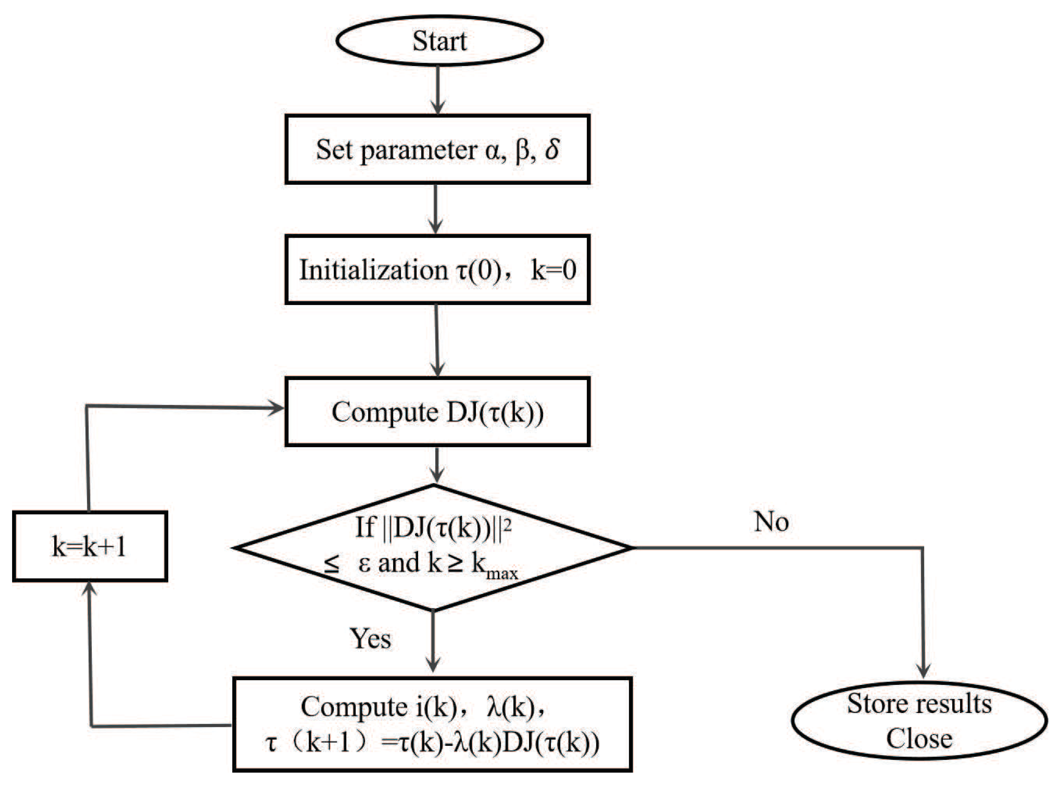
3.3. Optimal Fault Tolerant Algorithm
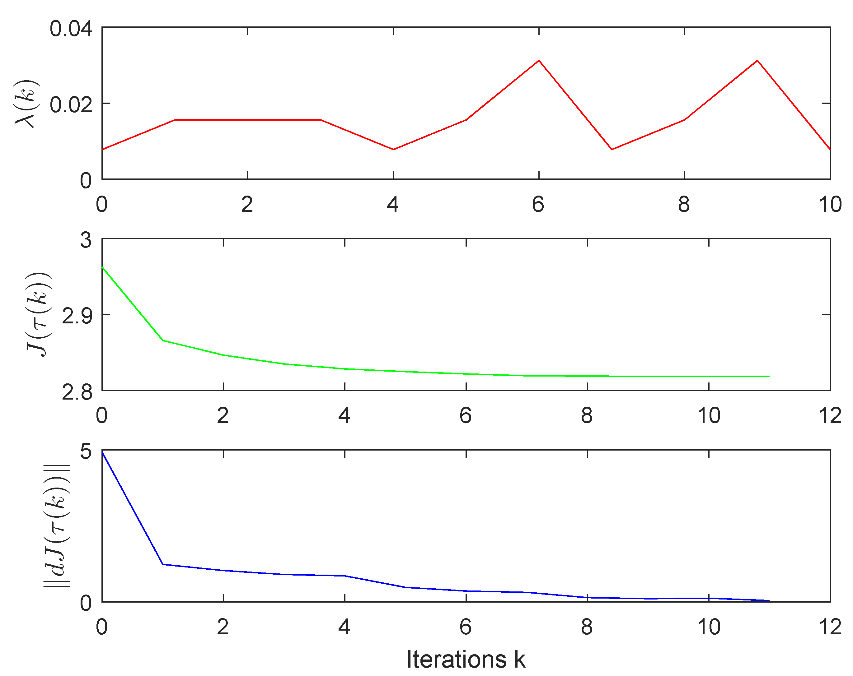
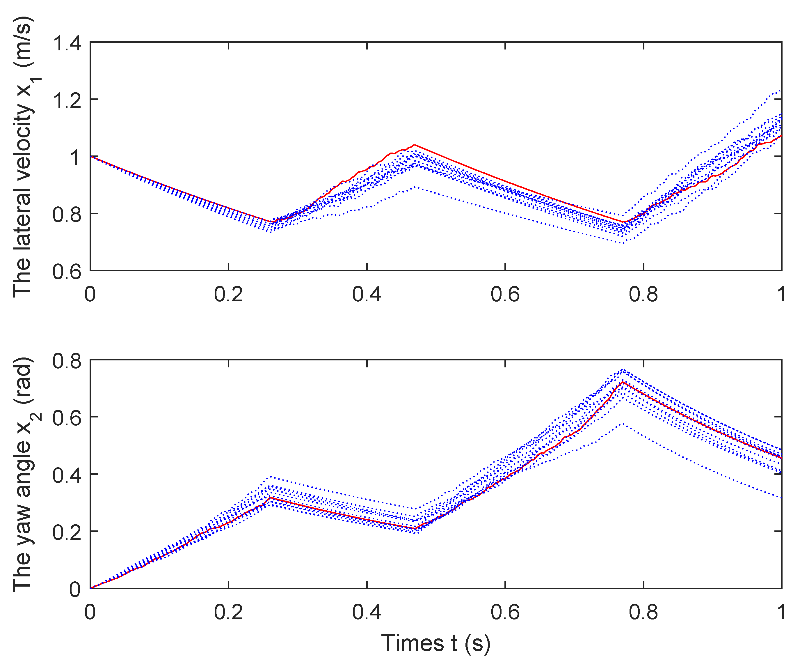
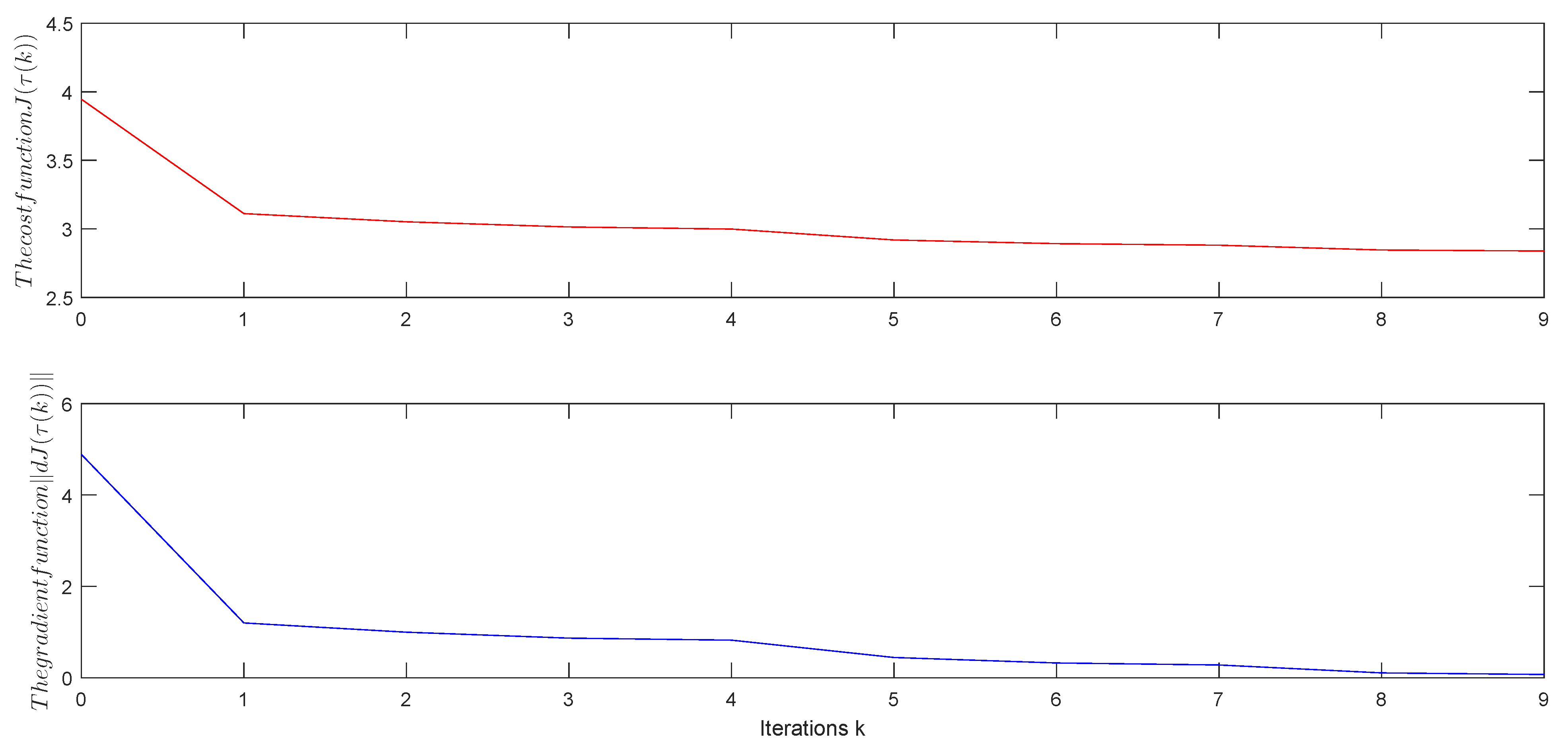
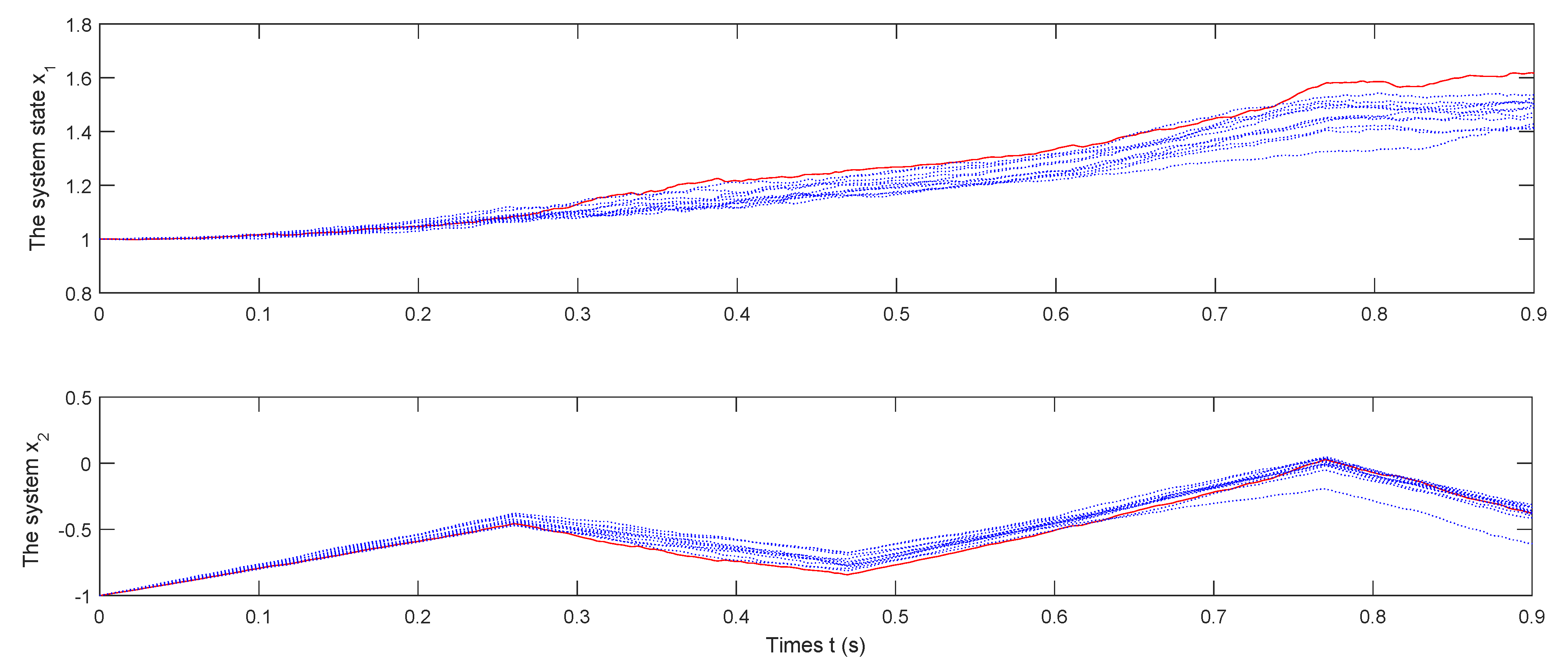
After taking into account the gradient of the cost functional in the above theorems, the next problem is to calculate the optimal switching time. In this subsection, the steepest descent algorithm with Armijo step sizes is explained in Figure 2. By denoting the initial parameters α ( 0 , 1 ) , β ( 0 , 1 ) and λ ( k ) : = β i ( k ) , the step size can be designed as i ( k ) = min { i 0 : J τ ( k ) β i D J ( τ ( k ) ) J ( τ ( k ) ) α β i D J ( τ ( k ) ) 2 } .

4. Simulation

In this section, the four wheel drive autonomous mobile robot system and numerical example are proposed to prove the feasibility of the designed optimization fault tolerant algorithm. The dynamic model of the four wheel drive mobile robot system represented in reference [35] is subject to actuator faults. It is shown that even with external stochastic disturbance and unknown switch draft fault in the actuator switched mechanism, the proposed optimization fault tolerant algorithm can explain the safety switch control of the different trajectory tasks for the autonomous mobile robot.

4.1. Practical Example

In consideration of the external stochastic disturbance, we select the lateral velocity and yaw angle of the center of gravity as the state variables. The kinematic model of the simplified four wheel drive mobile robot as shown in [35] is
a x = d V x d t V y d θ d t = V ˙ x V y Ω z , a y = d V y d t + V x d θ d t = V ˙ y + V x Ω z ,
where a x is the longitudinal acceleration, a y is the lateral acceleration, V x and V y are the forward velocity and lateral velocity of vehicle mass center, respectively, Ω z is the yaw motion around the Z axis. The mobile robot vehicle dynamics equation is as follows:
M a x = M V ˙ x V y Ω z = F x f cos δ f + F x r F y f sin δ f , M a y = M V ˙ y + V x Ω z = F y f cos δ f + F y r + F x f sin δ f , I z Ω ˙ z = l 1 F y f cos δ f l 2 F y r + l 1 F x f sin δ f ,
where δ f is the front wheel angle, F x f and F y f are the longitudinal and lateral forces of the front wheel, respectively. F x r and F y r are the longitudinal and lateral forces of the rear wheel, respectively. l 1 is the distance from the center of mass to the front axis, and l 2 is the distance from the center of mass to the rear axis. In consideration of the lateral characteristics of the tire, we have
F y f = C f α f , F y r = C r α r ,
where
α f = δ f l 1 Ω z + V y V x , α r = l 2 Ω z V y V x .
By substituting the kinematic model and the tire characteristics into the vehicle dynamics equation, we can obtain
V ˙ y = 1 M C f + C r V x V y V x + l 1 C f l 2 C r M V x Ω z + C f M δ f , Ω ˙ z = l 1 C f l 2 C r I z V x V y l 1 2 C f + l 2 2 C r I z V x Ω ˙ z + l 1 C f I z δ f .
The forward velocity of the mobile robot along the X axis is considered constant. Then, the car has only two degrees of freedom. In order to simplify the expressions, we introduce the change in coordinates:
a 11 = 1 M C f + C r V x , a 12 = V x + l 1 C f l 2 C r M V x , b 1 = C f M , a 21 = l 1 C f l 2 C r I z V x , a 22 = l 1 2 C f + l 2 2 C r I z V x , b 2 = l 1 C f I z , x 1 = V y , x 2 = Ω z .
By employing the external stochastic disturbance on the front wheel angle δ f , we select the coupling friction coefficients b 1 = 0 , b 2 = 1 and b 1 = 1 , b 2 = 0 to represent the the switched stochastic systems term B i ω . The forward velocity of the mobile robot along the X axis is considered constant. Thus, the four wheel drive mobile robot system has only two state variables, x 1 = V y , x 2 = Ω z . In complex road conditions, the friction coefficient of tires is different. In addition, we can note that the different trajectory tasks require a different forward velocity V x . Therefore, by different trajectory tasks, under the complex road conditions and external stochastic disturbance, the following switched stochastic systems equation is obtained for a four wheel drive mobile robot with safe trajectory planning:
x ˙ ( t ) = A 1 x ( t ) + B 1 ω , t [ t 0 , T 1 ] , A 2 x ( t ) + B 2 ω , t ( T 1 , t f ] ,
where the system matrices are
A 1 = 1 0 1 2 , B 1 = 0 1 , A 2 = 1 1 0 2 , B 2 = 1 0 .
As presented in the four wheel drive mobile robot example, the robot safe trajectory planning problems can be translated into the studied switched stochastic systems. Then, the proposed optimal timing fault tolerant control strategy can solve the safe trajectory planning problem effectively.
In order to illustrate the effectiveness of the proposed algorithm with multi-switching times, the system is repeatedly switched. The system is described by three switching points, as follows:
x ˙ ( t ) = A 1 x ( t ) + B 1 ω , t [ t 0 , T 1 ] , A 2 x ( t ) + B 2 ω , t ( T 1 , T 2 ] , A 1 x ( t ) + B 1 ω , t ( T 2 , T 3 ] , A 2 x ( t ) + B 2 ω , t ( T 3 , t f ] ,
where the initial state x ( 0 ) = [ 1 , 0 ] T , the initial time t 0 = 0 , the final time t f = 1 , the initial switching time T 1 = 0.3 , T 2 = 0.5 , T 3 = 0.7 . By the switch control mechanism, the four wheel drive mobile robot system executes the desired different trajectory tasks. We need to calculate the optimal switching time T 1 , T 2 , T 3 to minimize the cost functional J. The weight coefficient matrices are designed as the unit matrix. The steepest descent parameters are α = β = 0.5 , the threshold value ϵ = 0.05 , k m a x = 200 . The experiments are implemented with Matlab2015a on a desktop PC with i7-6700 3.4 GHz CPU, 16 GB memory and Windows 1064 bit OS. The simulation results are described in Figure 3 and Figure 4.
The optimal switching time is T = [ 0.2609 , 0.4677 , 0.7749 ] after ten iterations. Based on the proposed algorithm, we obtain the corresponding optimal cost J = 2.8185 . From Figure 3, it is easy to see that the cost J quickly converges to a minimum value and the gradient function d J ( τ ( k ) ) reaches the termination value. In addition, the system state trajectories with respect to the switching time signal τ ( k ) are illustrated in Figure 4.
The blue dotted lines explain the state trajectories with the iterate progress switching time vector τ ( k ) . As a comparison, the red solid line explains the optimal trajectories with respect to the optimal switching time signal.

4.2. Numerical Example

Consider the following switched nonlinear systems:
x ˙ ( t ) = A 1 x ( t ) + B 1 ω , t [ t 0 , T 1 ] , A 2 x ( t ) + B 2 ω , t ( T 1 , T 2 ] , A 3 x ( t ) + B 3 ω , t ( T 2 , T 3 ] , A 4 x ( t ) + B 4 ω , t ( T 3 , t f ] ,
where the system matrices are
A 1 = 1 1 0 2 , A 2 = 1 0 1 2 , A 3 = 1 0 1 2 , A 4 = 1 1 0 2
B 1 = B 3 = 0 1 , B 2 = B 4 = 1 0 .
We select the initial state x ( 0 ) = [ 1 , 1 ] T , the initial time t 0 = 0 , the final time t f = 0.9 , the initial switching time T 1 = 0.3 , T 2 = 0.5 , T 3 = 0.7 . The weight coefficient matrices are designed as Q 1 = I , Q 2 = 2 I , Q 3 = 3 I , Q 4 = 4 I , P = I , where I denotes the unit matrix. The cost function J ( τ ( k ) ) and the gradient function d J ( τ ( k ) ) with k iterations and the trajectories of the states x 1 ( t ) and x 2 ( t ) are shown in Figure 5 and Figure 6 when employing the proposed optimal timing fault tolerant control strategy.
It is worth noting that the switched subsystems are different in the numerical example which can describe the more general systems.

5. Conclusions

In this paper, an novel optimal timing fault tolerant control algorithm is proposed for switched stochastic systems with an unknown drift fault for each switching point. The designed optimal timing fault tolerant controller can not only realize the optimal performance, but also accommodate switching drift fault. Moreover, in this process, the cost functional has the general form with the integral terms and the terminal terms with the switched stochastic systems state variable. The variational technique is exploited to deduce the gradient formula. The steepest descent algorithm with Armijo step sizes is utilized to calculate the optimal switching time. The safety trajectory switching of a four wheel drive vehicle is taken as a practical application case to illustrate the effectiveness of the proposed method. Owing to the special structure of the gradient formula, how to extend the suggested methods to large-scale systems, multi-agent systems and practical systems are is a problem worthy of research.

Author Contributions

Conceptualization, C.Z.; methodology, C.Z., L.H. and K.Z.; software, C.Z. and L.H.; supervision, K.Z., W.S. and Z.H.; validation, C.Z., L.H. and Z.H.; writing, original draft, C.Z. and K.Z. All authors have read and agreed to the published version of the manuscript.

Funding

This work was funded by the Natural Science Foundation of China (No. 61973083, No. 61973077 and No. 61773118), and by the Fundamental Research Funds for the Central Universities: 2242022k30038.

Institutional Review Board Statement

Not applicable.

Informed Consent Statement

Not applicable.

Data Availability Statement

Not applicable.

Conflicts of Interest

The authors declare no conflict of interest.

References

  1. Geromel, J.C.; Colaneri, P. Stability and stabilization of discrete time switched systems. Int. J. Control 2006, 79, 719–728. [Google Scholar] [CrossRef]
  2. Wang, B.; Zhu, Q. Stability analysis of semi-Markov switched stochastic systems. Automatica 2018, 94, 72–80. [Google Scholar] [CrossRef]
  3. Zhao, Y.; Zhu, Q. Stabilization by delay feedback control for highly nonlinear switched stochastic systems with time delays. Int. J. Robust Nonlinear Control 2021, 31, 3070–3089. [Google Scholar] [CrossRef]
  4. Fan, L.; Zhu, Q. Mean square exponential stability of discrete-time Markov switched stochastic neural networks with partially unstable subsystems and mixed delays. Inf. Sci. 2021, 580, 243–259. [Google Scholar] [CrossRef]
  5. Bilbao, J.; Bravo, E.; García, O.; Rebollar, C.; Varela, C. Optimising energy management in hybrid microgrids. Mathematics 2022, 10, 214. [Google Scholar] [CrossRef]
  6. Ozkan, L.; Kothare, M.V. Stability analysis of a multi-model predictive control algorithm with application to control of chemical reactors. J. Process. Control 2006, 16, 81–90. [Google Scholar] [CrossRef]
  7. Hamouda, M.; Menaem, A.A.; Rezk, H.; Ibrahim, M.N.; Számel, L. Comparative evaluation for an improved direct instantaneous torque control strategy of switched reluctance motor drives for electric vehicles. Mathematics 2021, 9, 302. [Google Scholar] [CrossRef]
  8. Gao, F.; Wu, Y.; Zhang, Z. Global fixed-time stabilization of switched nonlinear systems: A time-varying scaling transformation approach. IEEE Trans. Circuits Syst. II Express Briefs 2019, 66, 1890–1894. [Google Scholar] [CrossRef]
  9. Zhu, F.; Antsaklis, P.J. Optimal control of hybrid switched systems: A brief survey. Discret. Event Dyn. Syst. 2015, 25, 345–364. [Google Scholar] [CrossRef]
  10. Li, S.; Qiu, J.; Ji, H.; Zhu, K.; Li, J. Piezoelectric vibration control for all-clamped panel using DOB-based optimal control. Mechatronics 2011, 21, 1213–1221. [Google Scholar] [CrossRef]
  11. Wu, X.; Zhang, K.; Cheng, M. Optimal control of constrained switched systems and application to electrical vehicle energy management. Nonlinear Anal. Hybrid Syst. 2018, 30, 171–188. [Google Scholar] [CrossRef]
  12. Fu, J.; Zhang, C. Optimal control of path-constrained switched systems with guaranteed feasibility. IEEE Trans. Autom. Control 2021, 67, 1342–1355. [Google Scholar] [CrossRef]
  13. Bai, Q.; Zhu, W. Event-triggered impulsive optimal control for continuous-time dynamic systems with input time-delay. Mathematics 2022, 10, 279. [Google Scholar] [CrossRef]
  14. Raisch, J.; O’Young, S.D. Discrete approximation and supervisory control of continuous systems. IEEE Trans. Autom. Control 1998, 43, 569–573. [Google Scholar] [CrossRef]
  15. Dong, J.; Yang, G.H. Robust static output feedback control synthesis for linear continuous systems with polytopic uncertainties. Automatica 2013, 49, 1821–1829. [Google Scholar] [CrossRef]
  16. Liu, T.; Qu, X.; Tan, W. Online optimal control for wireless cooperative transmission by ambient RF powered sensors. IEEE Trans. Wirel. Commun. 2020, 19, 6007–6019. [Google Scholar] [CrossRef]
  17. Stellato, B.; Oberblobaum, S.; Goulart, P.J. Second-order switching time optimization for switched dynamical systems. IEEE Trans. Autom. Control. 2017, 62, 5407–5414. [Google Scholar] [CrossRef] [Green Version]
  18. Seatzu, C.; Corona, D.; Giua, A.; Bemporad, A. Optimal control of continuous-time switched affine systems. IEEE Trans. Autom. Control 2006, 51, 726–741. [Google Scholar] [CrossRef]
  19. Azimi, M.; Sharifi, G. A hybrid control scheme for attitude and vibration suppression of a flexible spacecraft using energy-based actuators switching mechanism. Aerosp. Sci. Technol. 2018, 82, 140–148. [Google Scholar] [CrossRef]
  20. Yan, B.; Shi, P.; Lim, C.C.; Wu, C.; Shi, Z. Optimally distributed formation control with obstacle avoidance for mixed–order multi-agent systems under switching topologies. IET Control Theory Appl. 2018, 12, 1853–1863. [Google Scholar] [CrossRef]
  21. Ding, K.; Zhu, Q. Extended dissipative anti-disturbance control for delayed switched singular semi-Markovian jump systems with multi-disturbance via disturbance observer. Automatica 2021, 128, 109556. [Google Scholar] [CrossRef]
  22. Wu, K.; Yu, J.; Sun, C. Global robust regulation control for a class of cascade nonlinear systems subject to external disturbance. Nonlinear Dyn. 2017, 90, 1209–1222. [Google Scholar] [CrossRef]
  23. Zhang, M.; Zhu, Q. Stability analysis for switched stochastic delayed systems under asynchronous switching: A relaxed switching signal. Int. J. Robust Nonlinear Control 2020, 30, 8278–8298. [Google Scholar] [CrossRef]
  24. Liu, X.; Zhang, K.; Li, S.; Wei, H. Optimal timing control of discrete-time linear switched stochastic systems. Int. J. Control Autom. Syst. 2014, 12, 769–776. [Google Scholar] [CrossRef]
  25. Huang, R.; Zhang, J.; Lin, Z. Optimal control of discrete-time bilinear systems with applications to switched linear stochastic systems. Syst. Control. Lett. 2016, 94, 165–171. [Google Scholar] [CrossRef]
  26. Liu, X.; Li, S.; Zhang, K. Optimal control of switching time in switched stochastic systems with multi-switching times and different costs. Int. J. Control 2017, 90, 1604–1611. [Google Scholar] [CrossRef]
  27. Zhu, C.; Li, C.; Chen, X.; Zhang, K.; Xin, X.; Wei, H. Event-triggered adaptive fault tolerant control for a class of uncertain nonlinear systems. Entropy 2020, 22, 598. [Google Scholar] [CrossRef]
  28. Zhang, Y.; Jiang, J. Bibliographical review on reconfigurable fault-tolerant control systems. Annu. Rev. Control 2008, 32, 229–252. [Google Scholar] [CrossRef]
  29. Yu, X.; Jiang, J. A survey of fault-tolerant controllers based on safety-related issues. Annu. Rev. Control 2015, 39, 46–57. [Google Scholar] [CrossRef]
  30. Zhu, C.; Zhang, K.; Xin, X.; Gao, F.; Wei, H. Event-triggered adaptive fixed-time output feedback fault tolerant control for perturbed planar nonlinear systems. Int. J. Robust Nonlinear Control 2021, 31, 6934–6952. [Google Scholar] [CrossRef]
  31. Zhu, Q.; Cao, J. Exponential stability of stochastic neural networks with both Markovian jump parameters and mixed time delays. IEEE Trans. Syst. Man Cybern. Part B Cybern. 2010, 41, 341–353. [Google Scholar]
  32. Zhang, D.; Yu, L. Fault-tolerant control for discrete-time switched linear systems with time-varying delay and actuator saturation. J. Optim. Theory Appl. 2012, 153, 157–176. [Google Scholar] [CrossRef]
  33. Liu, J.; Zhang, K.; Sun, C.; Wei, H. Robust optimal control of switched autonomous systems. IMA J. Math. Control. Inf. 2016, 33, 173–189. [Google Scholar] [CrossRef]
  34. Guan, Y.; Yang, H.; Jiang, B. Fault-tolerant control for a class of switched parabolic systems. Nonlinear Anal. Hybrid Syst. 2019, 32, 214–227. [Google Scholar] [CrossRef]
  35. Peng, S.T. On one approach to constraining the combined wheel slip in the autonomous control of a 4ws4wd vehicle. IEEE Trans. Control. Syst. Technol. 2006, 15, 168–175. [Google Scholar] [CrossRef]
Figure 1. Switching times within the time grid.
Mathematics 10 01880 g001
Figure 2. The steepest descent algorithm flow chart.
Mathematics 10 01880 g002
Figure 3. The designed step size λ ( k ) , the cost functional J ( τ ( k ) ) and gradient d J ( τ ( k ) ) with k iterations.
Mathematics 10 01880 g003
Figure 4. The trajectories of states x 1 ( t ) and x 2 ( t ) .
Mathematics 10 01880 g004
Figure 5. The cost function J ( τ ( k ) ) and the gradient function d J ( τ ( k ) ) with k iterations.
Mathematics 10 01880 g005
Figure 6. The trajectories of states x 1 ( t ) and x 2 ( t ) .
Mathematics 10 01880 g006
Publisher’s Note: MDPI stays neutral with regard to jurisdictional claims in published maps and institutional affiliations.

