Low-Cost Emergent Dynamic Scheduling for Flexible Job Shops

Abstract

Flexible production is a typical representative of high-end manufacturing and is also a manifestation of a country’s national production capability. Compared with other production modes, the key distinction of flexible production is that all four dimensions of production (i.e., machines, operations, products, and orders) can be scheduled dynamically. Although many studies have investigated the flexible job shop scheduling problem, most have limited dynamic support and cannot deal with multidimensional dynamic production. This study, therefore, proposed a fine-grained system state description model, which was used to analyze the maximum production completion time. In the presence of a dynamic event, the model was able to quickly assign priorities to products according to the cost loss of each product. The system can therefore dynamically respond to events in a timely manner while reducing production costs and losses. Finally, we used a large number of orders to evaluate the proposed algorithm, which demonstrated millisecond-level response capability and low-cost maintenance capability. Compared with existing algorithms, the proposed algorithm reduced cost loss by up to $11\%$.

1. Introduction

Flexible production is a typical representative of high-end manufacturing. Here, “flexible” refers to the flexibility consumers have in customizing products. Compared with traditional production methods in which consumers can only purchase finished products, flexible production can quickly meet the individual needs of different consumers. In traditional production, cost reduction is achieved through mass production, which means it often cannot support customization. Although customization is possible for a small number of production methods, the associated production cost is usually high. With the rapid development of various technologies in recent years, such as industrial Internet, robots, and edge computing, the dynamic self-reconfiguration of production lines has become an option. Low-cost, flexible production has overcome the technical bottleneck, and an increasing number of flexible job shops have been put into use, achieving considerable economic benefits [1]. As an example, the flexible job shop in a Chinese heavy equipment manufacturing company, is equipped with eight assembly lines, which can achieve customized production for 69 types of products, showing a threefold increase in output value.

A flexible job shop contains multiple production lines, and each is composed of multiple machines. To make our proposed algorithm applicable to more industrial systems, our system model is defined broadly. Although there is a strict order for all operations in a job, multiple operations may be executed on the same machine, i.e., the job may not follow a linear fashion. Hence, our problem is not a flow shop scheduling problem. Details are shown in Section 4. In our system, after a customer’s order is received, the machines are reconfigured and scheduled according to customization needs and delivery time, such that the production process can be dynamically adjusted to meet order demand. As a result of different order-specific requirements, random order placement times, and the large number of machines, simple production scheduling can no longer meet production needs in such complex situations. Therefore, flexible job shop scheduling has become a key issue in the industry and has been investigated by numerous studies.

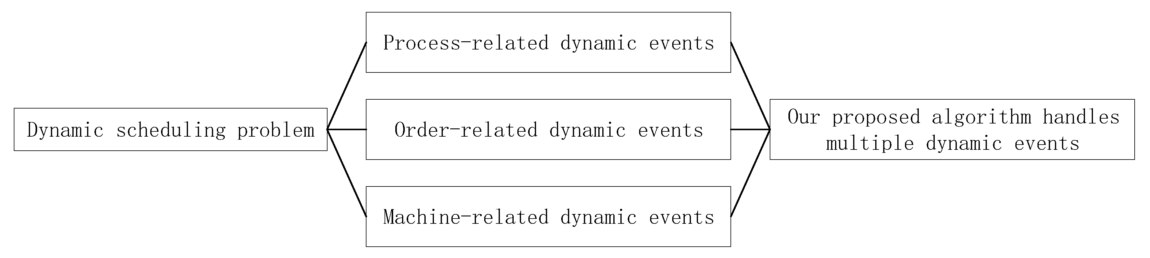
In an industrial system, there are many types of dynamic events, such as process-related, order-related and machine-related dynamic events. However, no algorithm can handle multiple dynamic events simultaneously (shown in Section 2). Therefore, in this study, a time-fine-grained state model was used to represent the complete characterization of system dynamics, and the model allowed changing the relationship between products and orders. Based on the time-fine-grained model and the flexible correspondence between products and orders, aiming at the lowest cost loss, a theoretical description of the optimization problem was given, and a priority scheduling algorithm based on completion time analysis was proposed to realize emergent scheduling to meet production needs. Since the model described the system state in a time-discrete manner and transformed the states at different times through our proposed efficient algorithm, this study can flexibly respond to multiple dynamic events.

The remainder of this paper is organized as follows. Section 2 introduces relevant works. Section 3 details the system model and our problem. Section 4 describes our algorithms. Section 5 evaluates the algorithms based on extensive orders. Finally, Section 6 concludes this paper.

2. Relevant Works

For the flexible job shop problem, there are two types of scheduling algorithms, namely static scheduling algorithm and dynamic scheduling algorithm.

In 1954, Johnson formulated the job shop scheduling problem and proposed the first static scheduling algorithm [2]. Static scheduling means that the production process is determined and there are no dynamic events. Since then, the static scheduling problem has been extensively studied. In the case of a single-objective static scheduling problem, improved meta-heuristic algorithms have typically been used to minimize the maximum completion time [3,4], number of machines [5], and machine usage time [6]. However, a flexible job shop involves a large number of complex processes, and multi-objective optimization has also been a key research topic in flexible scheduling. For example, an evolutionary algorithm has been used to simultaneously optimize completion time, energy consumption, and cost [7]. An improved multi-group NSGA-II algorithm was used to simultaneously optimize completion time, machine efficiency, and total machine load [8]. Further, hybrid particle swarm optimization was used to optimize completion time and total machine delay [9]. One study used the genetic algorithm to optimize total machine load and bottleneck machine load [10]. Meanwhile, Change et al. used the concept of “residual value subsidy + out-of-stock penalty” to optimize the economic benefits of multiple enterprises at the same time [11]. Wu et al. used the batch rolling optimization method to optimize production processes and production plans [12]. All of the above-mentioned studies regarded machines as the scheduling resources. Some studies have considered automatic guided vehicles as movable resources for optimization. For example, considering both automatic guided vehicles and machines, one study proposed using discrete particle swarm optimization to minimize the maximum completion time [13]. Considering the working capacity limitations of automatic guided vehicles, Li et al. proposed an artificial bee colony optimization algorithm for the multi-objective optimization of completion time and energy consumption [14]. These studies solved some of the scheduling problems in flexible job shops but failed to consider the dynamic situation of sudden production needs. One of the prerequisites of flexible job shops is that the production process can be dynamically adjusted to produce efficiently according to demand.

In 1957, Jackson distinguished the difference between dynamic scheduling and static scheduling, and he pointed out that the main feature of dynamic scheduling is to consider dynamic events [15]. In terms of the dynamic scheduling problem, researchers have conducted studies from multiple perspectives [16]. For process-related dynamic events, Wei et al. proposed a closed-loop scheduling mechanism for detection and adjustment based on the brainstorming algorithm to ensure completion time [17]. Li et al. proposed a novel affinity calculation method to handle high levels of uncertainty [18]. Xu et al. proposed an adaptive discrete flower pollination algorithm to handle the uncertainty of parameters during a flexible industrial process [19]. Zhong et al. proposed a new artificial bee colony algorithm to minimize the maximum fuzzy makespan [20]. Lei proposed a random key genetic algorithm to solve job shop scheduling problems with fuzzy processing time [21]. Liu et al. proposed a fast distribution estimation algorithm [22]. For order-related dynamic events, Luo et al. employed reinforcement learning-based methods to dynamically adjust production processes [23]. Luo and Wang proposed a double loop deep Q-network method with an exploration loop and exploitation loop to solve job shop scheduling problems under random order arrivals [24,25]. Zhuang et al. proposed a network-based dynamic dispatching rule generation mechanism to assign dynamic orders [26]. For machine-related dynamic events, scheduling must consider the cost of machine recovery; a few algorithms have been proposed to deal with this problem. Nouiri et al. proposed a fast, energy-efficient rescheduling method [27], and Chen et al. proposed a machine parameter readjustment method based on knowledge libraries and self-learning [28,29]. Zhang et al. designed an improved empire competition algorithm to minimize completion time and machine energy consumption while repairing the machine [30]. Shahrabi et al. used a machine learning algorithm to achieve real-time production scheduling [31]. Ghaleb et al., meanwhile, adopted an event-based rescheduling approach to address uncertainties in job arrivals and machine breakdown [32]. A predictive approach was proposed by Iwona et al. to deal with possible failures before they occur [33].

Although the above-mentioned studies investigated the dynamics of flexible job shops, they have some limitations. In actual production, unpredictable dynamic events such as machine breakdown, product defects, and order changes may arise, and any existing single algorithm is unable to deal with multiple events (as shown in Figure 1). Although the likelihood of multiple events occurring at the same time is very low, this still requires the system to support multiple scheduling methods. Thus, when a single dynamic event occurs, the scheduling method for the specific event can be used to solve it. However, the scheduling methods must be coordinated with each other. Otherwise, the results of one scheduling method will compromise existing scheduling outcomes. Therefore, compared with multiple scheduling algorithms, it is more effective to use one scheduling algorithm to handle multiple dynamic events. In this study, such a scheduling algorithm is proposed.

3. Problem Statement

We considered the dynamic problem model in four dimensions: machines, operations, products, and orders. The machine set available to the job shop is $M=\{m_1,m_2,\dots \}$, and the set of supported operations is $O=\{o_1,o_2,\dots \}$. Each machine supports several operations—for example, $m_j=\{o_{j,1}^m,o_{j,2}^m,\dots \}$. Operations corresponding to the machine are marked with a superscript m to distinguish them from the original operation set O (i.e., $o_{j,g}^m\in O)$. However, $o_{j,g}^m$ might not be equal to $o_g$ ($g\in Z^{+}$). It takes $t_h^o$ time to complete the operation $o_h$ ($h\in Z^{+}$). The product set is $P=\{p_1,p_2,\dots \}$, and each product is produced after multiple steps of sequential operations, $p_k=\{o_{k,1}^p,o_{k,2}^p,\dots \}$. The user can place an order $q_i=<p_i^q,d_i>$ at any time, and the order specifies the product $p_i^q$ and the latest delivery time $d_i$. The product $p_i^q$ consists of a series of operations, $p_i^q=\{o_{i,1}^q,o_{i,2}^q,\dots \}$. The set of orders is expressed as $Q=\{q_1,q_2,\dots \}$. The state model of the job shop at time t is $S_t=\{<m_j,p_k,o_{k,g}^p,t_j^r>|m_j\in M\mathrm{or}{m}_j=NULL,p_k\in P\mathrm{or}{p}_k=NULL,o_{k,g}^p\in p_k,t_j^r\in [0,t_h^o]\}$, where each quadruple means that machine $m_j$ is performing the gth operation of product pk at time t, and the operation has been performed for $t_j^r$ time. Note that some products might already be in the production plan, but the production has not yet started, and this state is expressed as $<NULL,p_k,o_{k,g}^p,t_j^r>$. When the production plan of some products is canceled, the state is expressed as $<NULL,p_k,o_{k,g}^p,0>$. If a machine is idle, its state is represented as $<m_j,NULL,NULL,0>$. Once some operations are interrupted, they need to be restarted, and for such operations, $t_j^r=0$. The above states can be jointly expressed using $S_t$; special algorithmic processing is not needed, and thus, they will not be considered in the sections that follow.

The system model includes the following assumptions:

• All pieces have arrived before the operation starts.
• The next operation cannot be started until the current operation is completed for the same product.
• There is no time gap between adjacent operations for the same product.

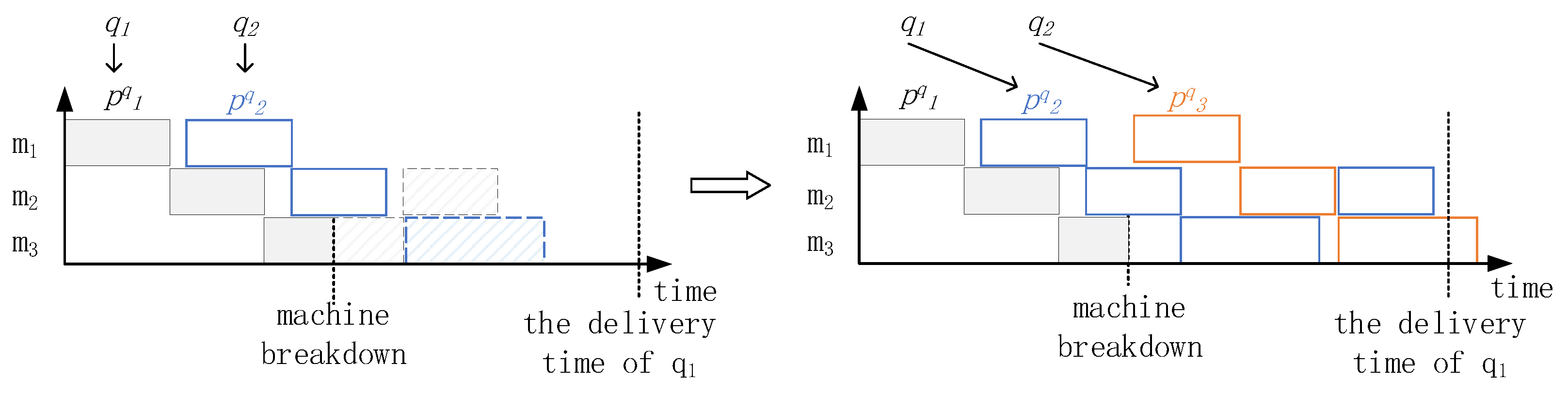
This study separated products and orders to flexibly adjust operations during the production process. While product demand comes from orders, products can be adjusted at the operation level when dynamic events occur. For example, in Figure 2, the semifinished product $p_1^q$ in order $q_1$ is damaged due to machine breakdown in the third operation, and product delivery cannot be guaranteed within the specified time in the case of reproduction. In this case, if there is product $p_2^q$ in the same operation as the operation of $p_1^q$, and the delivery time of $p_2^q$ is later, then the subsequent operation of product $p_2^q$ is adjusted to that of product $p_1^q$ such that order $q_1$ can be delivered on time. At the same time, a new $p_2^q$ is reproduced. Based on the idea of product–order separation, the scheduling method in this study generates a subsequent schedule $Sch(S_t,t)$ according to the shop state $S_t$ at time t. Products produced according to this schedule must meet the delivery requirements of the order set Q as much as possible, with minimum cost loss. The cost loss of order $q_i$ failure is expressed as $C\left(q_i\right)$, which includes the cost of reproduction, the cost of machine repair and maintenance, and compensation to consumers. The cost loss can be defined by the user of the algorithm.

To clearly describe the above problems, we first present problem description P1 based on optimization modulo theories (OMT) at the start of the system; subsequently, the description is expanded to the handling of dynamic events to formalize the final problem description P2. This study used the following 0–1 variable to describe the relationship between elements, as shown in Figure 3.

1.

If order $q_i$ has no deliverable product at the final delivery time, then $e_i=1$; otherwise, $e_i=0$.

2.

If product $p_k$ is available for the delivery of order $q_i$, then $x_{i,k}=1$; otherwise, $x_{i,k}=0$.

3.

If the operation $o_{k,g}^p$ of product $p_k$ can start on $m_j$ at time t, then $y_{k,g,t,j}=1$; otherwise, $y_{k,g,t,j}=0$.

4.

If the gth operation of product $p_k$ is $o_h$, then $z_{k,g,h}=1$; otherwise, $z_{k,g,h}=0$. This variable enables the product to change the final product type according to the needs of dynamic events.

First, we consider the situation at the start of the system. The set of orders Q, set of machines M, set of products P, and cost loss value $C\left(q_i\right)$ ($\forall q_i\in Q$) are known. All machines are idle, and there is no product currently in the production process. The objective function of problem P1 is

$$min\sum _{\forall q_i\in Q}C\left(q_i\right)\times e_i,$$

(1)

where $e_i$ can be obtained by $x_{i,k}$:

$$\forall q_i\in Q,((e_i=1)\wedge (\underset{\forall p_k}{\wedge }(x_{i,k}=0)))\vee ((e_i=0)\wedge (\underset{\forall p_k}{\vee }(x_{i,k}=1))).$$

(2)

The value of $e_i$ is divided into two cases: (1) If all products cannot be delivered as part of order $q_i$ (i.e., $\underset{\forall p_k}{\wedge }(x_{i,k}=0)$), then $e_i=1$. (2) If there are products that can be delivered for order $q_i$, (i.e., $\underset{\forall p_k}{\vee }(x_{i,k}=1)$), then $e_i=0$.

Problem P1 needs to satisfy the following constraints:

(1) One product can only be delivered for one order:

$$\forall p_k\in P,\sum _{\forall q_i\in Q}{x}_{i,k}=1.$$

(3)

(2) One operation can only be performed on one machine:

$$\forall p_k\in P,\forall o_{k,g}^p\in p_k,\sum _{\forall t,\forall m_j}{y}_{k,g,t,j}=1.$$

(4)

(3) Each operation of a product is unique:

$$\forall p_k\in P,\forall g,\sum _{\forall h\in [1,|O\left|\right]}{z}_{k,g,h}=1.$$

(5)

(4) Only products that meet the requirements of the order can be used for order delivery; that is, the operation steps and sequences of the product are exactly the same as those of the order requirements:

$$\forall q_i\in Q,\forall p_k\in P,\underset{\forall g}{\wedge }(o_{i,g}^q=\sum _{\forall o_h\in O}(z_{k,g,h}\times h))\wedge (x_{i,k}=1).$$

(6)

(5) There are no conflicts regarding machine usage time. The usage time of operation $o_{k,g}^p$ on machine $m_j$ is defined as $[{\alpha }_{k,g,j},{\beta }_{k,g,j}]$:

$$\forall m_j\in M,{\alpha }_{k,g,j}=\sum _{\forall t}t\times y_{k,g,t,j},{\beta }_{k,g,j}={\alpha }_{k,g,j}+t_{k,g}^p.$$

(7)

If an operation does not involve the use of machine $m_j$, then its usage time is expressed as $[0,0]$. Any two operations on the same machine cannot overlap in time:

$$(o_{k,g}^p=o_{a,b}^p)\vee ([{\alpha }_{k,g,j},{\beta }_{k,g,j}]=[0,0])\vee ([{\alpha }_{a,b,j},{\beta }_{a,b,j}]=[0,0])\vee ([{\alpha }_{k,g,j},{\beta }_{k,g,j}]\cap [{\alpha }_{a,b,j},{\beta }_{a,b,j}]=\varnothing ).$$

(8)

(6) Multiple steps for a product must be operated in sequence; that is, the completion time of the previous step must be earlier than the start time of the subsequent step:

$$\forall p_k\in P,\forall g\in [1,|p_k\left|\right),\sum _{\forall m_j\in M}{\beta }_{k,g,j}<\sum _{\forall m_j\in M}{\alpha }_{k,g+1,j}.$$

(9)

(7) The product must be completed before delivery; that is, the completion time of the last step of the product must be earlier than the order delivery deadline:

$$\forall q_i\in Q,\forall p_k\in P,(x_{i,k}=0)\vee (\sum _{\forall m_j\in M}{\beta }_{k,|p_k|,j}\le x_{i,k}\times d_i).$$

(10)

The state at time t is denoted $S_t$. If a dynamic event causes production to fail, such as the machine breakdown in Figure 2, the product is removed from $S_t$. If the order is canceled, it is removed from the set of orders. Based on the type of dynamic event, the following three modifications are made to problem P1 so that it can describe scheduling problem P2 after the occurrence of the dynamic event:

(1) The elements in $S_t$ that do not include $NULL$ indicate that the operation has been executed on the machine, and the corresponding $y_{k,g,t,j}$ and $z_{k,g,h}$ cannot be changed or optimized. Therefore, $y_{k,g,t,j}$ and $z_{k,g,h}$ are given fixed values, and the constraints on related operations are removed from the problem description:

$$\forall <m_j,p_k,o_{k,g}^p,t_j^r>\in S_t,y_{k,g,t-t_j^r,j}=1,$$

(11)

$$\forall <m_j,p_k,o_{k,g}^p,t_j^r>\in S_t,\forall h\in [1,o_{k,g}^p],z_{k,g,h}=1.$$

(12)

In addition, although the values of ${\alpha }_{k,g,j}$, ${\beta }_{k,g,j}$, and other $y_{k,g,t,j}$ are also affected, they can be calculated by Equations (4) and (7).

(2) If a product fails to be produced and needs to be reproduced, a corresponding number of products need to be added to P. Since the production steps for the additional products can be obtained in the algorithm, there is no need for constraints on product type.

(3) If an order is canceled, it is removed from Q.

This study focused on scheduling problem P2 after the occurrence of dynamic events. If the decision version of the problem does not consider the situation in which products can be transferrable to other orders, and the delivery time of all orders is limited to the shortest schedulable time, then the decision problem can be reduced to the traditional job shop scheduling problem. Since the job shop scheduling problem is an NP-hard problem, problem P2 is at least NP-hard, and the optimal solution cannot be obtained in polynomial time.

To validate the above model, we used a third-party solver Microsoft Z3 [34] to solve it. However, owing to the complexity of the model, the optimal solution can only be found within two hours for very small-scale variables. Since the focus of this study was emergency responses to dynamic events, the algorithm needed to be able to provide solutions within seconds or even milliseconds. Apparently, the hour-level algorithm cannot meet these requirements. This study, therefore, proposed a fast heuristic algorithm, which is described in the next section.

4. Scheduling Algorithm

An efficient priority scheduling strategy was adopted to achieve fast responses. First, assuming the priorities of all products have been assigned, a detailed priority scheduling algorithm is proposed. Then, the relationship between priority and product production time is analyzed using the scheduling algorithm. Lastly, priorities are assigned to products according to the above relationship, and production scheduling is achieved based on the priority scheduling algorithm.

Priority Scheduling

The priority of product $p_k$ is ${\rho }_k$ (priority assignment will be discussed later. In Algorithm 1, we assume ${\rho }_k$ is known.). Figure 4 shows the main steps for priority scheduling. For each operation, there is a product queue in which products are arranged from high to low priority. Once the machine completes an operation for a product, it continues to perform the operation on the next product with the highest priority in the queue, and the queue is updated. If multiple products are in the queue for machine $m_j$, and product $p_k$ has the highest priority, then $p_k$ is processed first. The corresponding scheduling algorithm is as shown in Algorithm 1.

Algorithm 1: Scheduling algorithm based on priority assignment

Input:$S_{ct}$ Output:$\forall y_{k,g,t,j}$, $obj$ 1: The elements in Q are sorted. For $q_i$ and $q_v$, if $d_i<d_v$, then $q_i$ is in front of $q_v$. The sorted set is $Q’$, where $q{’}_1$ has the shortest deadline. 2: for each $q{’}_i$ from $q{’}_1$ to $q{’}_{\left|Q\right|}$ do 3:    Search for product $p_k$ in P belonging to other undelivered orders, and the completed operation of $p_k$ in P is exactly the same as the previous operation of $q{’}_i$, and $p_k$ is the product with the maximum number of completed operations; 4:    $p_k$ will be delivered to order $q{’}_i$, i.e., $x_{i,k}=1$; 5:    Update the subsequent operations of $p_k$ according to order $q{’}_k$, that is, value assignment for $z_{k,g,h}$. 6:    Initialize order delivery status, i.e., $e_i=1$; 7: $AssignPriority\left(\right)$; // assign priority k for each product (Algorithm 2) 8: for$t=ct$ to ${max}_{\forall q_i\in Q}\left\{d_i\right\}$ do 9:    for $\forall m_j\in M$ do 10:      if $m_j$ is idle then 11:         $m_j$ processes $p_k$, $p_K\in Ps\left(m_j\right)$ and $/\exists p_u\in Ps\left(m_j\right)$ such that ${\rho }_b>{\rho }_k$, i.e., $y_{k,g,t,j}=1$; 12:      if $m_j$ finishes the operation for $p_k$ then 13:         $m_j$ is idle; 14:         Find the next operation for $p_k$ according to $z_{k,g,h}$, and put it in the waiting lists of the next operation; 15:         if $p_k$ is completed then 16:           if $t\le d_i$ then 17:              Order is deliverable, i.e., $e_i=0$; 18: Calculate $obj$ based on $e_i$ using Equation (1); 19: return $\forall y_{k,g,t,j}$, $obj$;

The input of Algorithm 1 is the fine-grained system state model $S_{ct}$, and the output is the scheduling result and the optimization objective for the problem. The system breaks down at time $ct$, and the problem model is modified from the three aspects of P2 and is input into the scheduling algorithm as the known input of Algorithm 2. After a series of processing, the scheduling result $y_{k,g,t,j}$ and objective $obj$ are output. The algorithm needs to first determine the correspondence between orders and products (lines 1–6) and process orders based on their priorities (lines 1–2). For order $q_i$, search for a deliverable product $p_k$ in P (line 3); the product must satisfy two conditions: (1) The completed steps of $p_k$ before time $ct$ must be completely consistent with the steps of order $q_i$; that is, Equation (6) is true before time $ct$. (2) Compared with product $p_k$, there is no other product that has more steps than $q_i$. Then, according to the identified product $p_k$, initial values are assigned to the order–product relation $x_{i,k}$, further operations $z_{k,g,h}$ of $p_k$, and order undelivered indicator $e_i$ (lines 4–6). After that, Algorithm 2 is used to assign priority to each product (line 7). Once the relationship between order, product, and priority is determined, products and operations are assigned to each machine in chronological order (lines 8–17). If machine $m_j$ is idle at the current moment, find the $p_k$ with the highest priority that can be processed on this machine (lines 10–11), where $Ps\left(m_j\right)$ is the set of products that can be processed on $m_j$—that is, $Ps\left(m_j\right)=\left\{p_a\right|z_{a,g,h}=1,o_h\in m_j\}$. When $m_j$ completes the current operation (line 12), its state is set to idle to wait for a new product at the next moment (line 13), and $p_k$ enters the queue for the next operation (line 14). If all operations of $p_k$ are completed before the deadline (lines 15–16), the product can be successfully delivered, and the undelivery indicator $e_i$ is cleared (line 17). When it is traversed in a finite time, the objective of the problem is calculated according to Equation (1) (line 18), which is output to the general control unit of the system together with the scheduling result (line 19). The algorithm is called each time a dynamic event occurs. After that, the general control unit schedules the production process according to the algorithm’s results.

In Algorithm 1, apart from Algorithm 2, the parts with the highest time complexity are lines 8, 9, and 11, and the corresponding time complexities are $O\left(t\right)$, $O\left(\right|M\left|\right)$, and $O\left(\right|P\left|\right)$, respectively. Thus, without considering Algorithm 2, the time complexity of Algorithm 1 is $O\left(t\right|M\left|\right|P\left|\right)$ (i.e., $O\left(n^3\right)$).

Algorithm 2: Priority assignment algorithm $AssignPriority\left(\right)$

Input:  $S_{ct}$ Output:  $\forall {\rho }_k$ 1: $\rho =0$; $\overline{\rho }=\left|P\right|$; 2: while$\rho \ne \overline{\rho }$do 3:    for $\forall p_k\in P$ do 4:      Assume $p_k$ is the product with the least priority in P, and calculate ${\delta }_k$ using Equation (13); 5:      ${\widehat{\delta }}_k={\displaystyle \sum _{\forall q_i\in Q}}{x}_{i,k}\times d_i-{\delta }_k$; 6:    Find the maximum ${\delta }_k$; 7:    if ${\delta }_k<0$ then 8:      The current priority $\rho$ is assigned to the product with the least cost loss, and it is removed from P; 9:    else 10:      The current priority $\rho$ is assigned to the corresponding product $p_k$, i.e., ${\rho }_k=\rho$; remove $p_k$ from P; 11:    $\rho =\rho +1$; 12: return$\forall {\rho }_k$;

5. Numerical Analysis

5.1. Time Analysis

Based on Algorithm 2, this section analyzes the maximum production completion time of product $p_k$, thereby obtaining the correspondence between the priority and deliverability of the product. For product $p_k$, it is defined that an operation to be performed at the current time $ct$ is $o_{k,c}^p$. Starting from the current time $ct$, in the worst case, it will take k time to complete the production. k is affected by the following factors: (1) the remaining time of the previous operation $o_{k,c-1}^p$; (2) the operation being performed on the machine at time $ct$ and the delay caused by $p_k$ not being ready; (3) the product with a higher priority than $p_k$ will be processed on the machine first, causing $p_k$ to be delayed; and (4) the operation time of $p_k$. Starting from time $ct$, for each operation between the first operation $o_{k,c}^p$ and the last operation $o_{k,|p_k|}^p$ of $p_k$, Factors (2)–(4) may exist. Thus, it will take the time described by Equation (13) at most to complete $p_k$:

$${\delta }_k=A_k+\sum _{\forall o_{k,g}^p\in \{o_{k,c}^p,...,o_{k,|p_k|}^p\}}(\frac{B_{k,g}+C_{k,g}}{|Ms(o_{k,g}^p)|}+D_{k,g}),$$

(13)

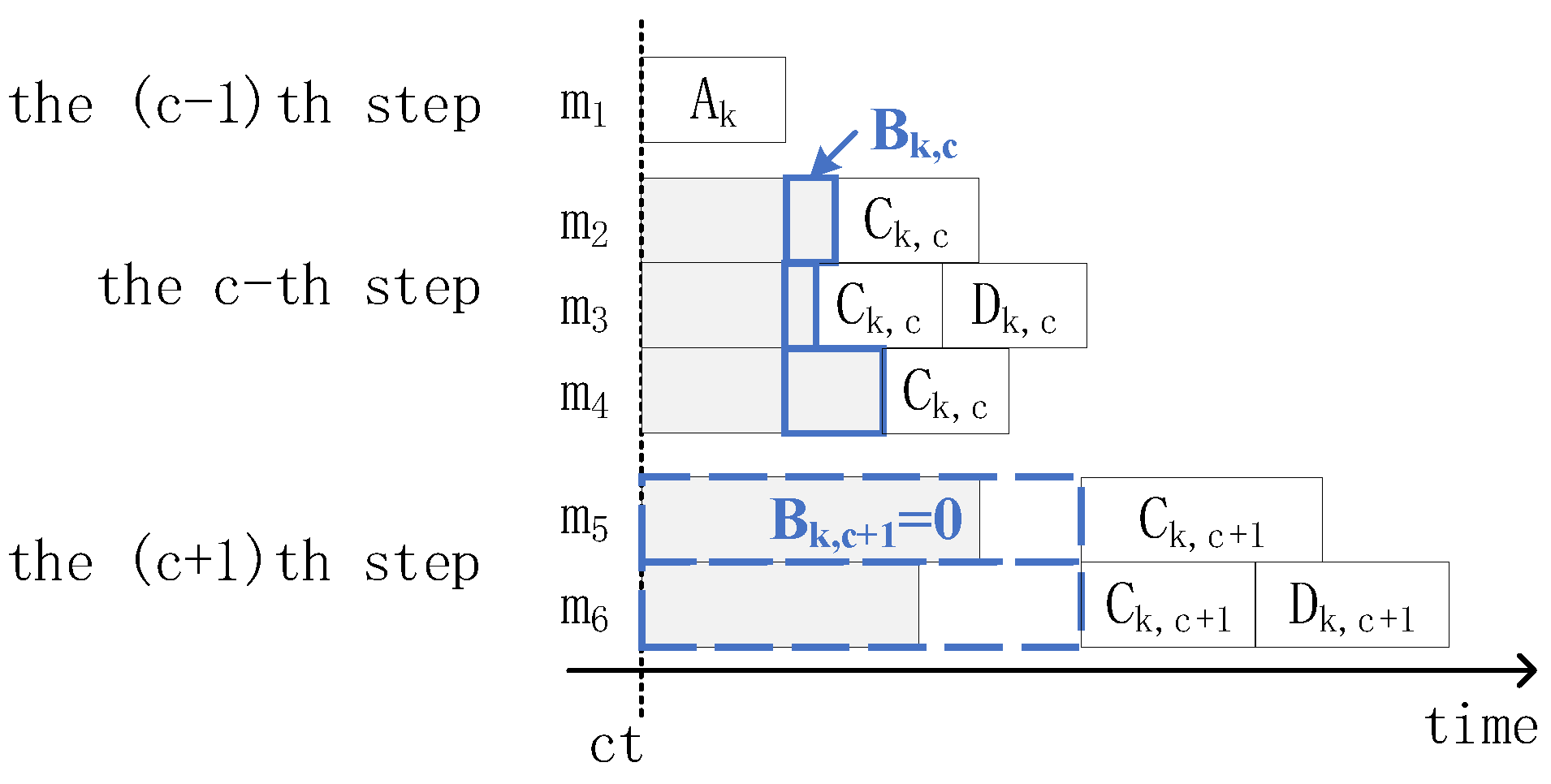
where $Ms\left(o_{k,g}^p\right)$ is the set of machines that support the operation $o_{k,g}^p$; $A_k$ is the time of Factor (1); and $B_{k,g}$, $C_{k,g}$, and $D_{k,g}$ are the time of Factors (2)–(4) of the gth step. Based on Figure 5, time k is described as follows:

If an operation of $p_k$ has started before time $ct$, the remaining time of the operation does not exceed the overall time of the operation. Thus, $A_k$ can be expressed as

$$A_k=\left\{\begin{array}{c}{t}_{k,c-1}^p-1\mathrm{if}\exists o_{k,c-1}^p,\hfill \\ 0\mathrm{otherwise}.\hfill \end{array}\right.$$

(14)

From the second operation, each operation can be executed on multiple machines. The factors that might cause a production delay of $p_k$ of multiple machines are expressed as $B_{k,g}+C_{k,g}$. After completing the previous operation, $p_k$ will wait for the next operation on the machine that is available first. Although the earliest available time of B and C cannot be estimated, the time will not exceed the average running time of B and C on multiple machines, which is $(B_{k,g}+C_{k,g})/|Ms(o_{k,g}^p)|$. The time delay of Factor (2) starts from time $ct$. To accumulate the time delay in multiple steps, $B_{k,g}$ only represents the time elapsed since the end of the previous operation, such as step c in Figure 5. If the time delay of Factor (2) does not exceed the end time of the previous operation, then $B_{k,g}=0$ (step $c+1$ in Figure 5). The end time of the previous operation is expressed as

$$E_{k,g-1}=A_k+\sum _{\forall o_{k,u}^p\in \{o_{k,c}^p,...,o_{k,g-1}^p\}}(\frac{B_{k,u}+C_{k,u}}{\left|Ms\right(o_{k,u}^p\left)\right|}+D_{k,u}).$$

(15)

The overall delay caused by factor (2) is expressed as

$$F_{k,g}=MaxT(|Ms(o_{k,g}^p)|,Os(Ms(o_{k,g}^p)))+MaxT(|Ms(o_{k,g}^p)|,Lp(Ms(o_{k,g}^p))),$$

(16)

where $Os(Ms(o_{k,g}^p))$ is the unfinished operation on machine $Ms(o_{k,g}^p)$, and $Lp(Ms(o_{k,g}^p))$ is the operation that will be performed on $Ms(o_{k,g}^p)$, which has a smaller priority than $o_{k,g}^p$. $MaxT(number,set)$ is the sum of the execution time of number operations with the longest execution time in the set. Therefore, $B_{k,g}$ is calculated as follows:

$$B_{k,g}=max\{0,F_{k,g}-|Ms(o_{k,g}^p)|\times E_{k,g-1}\}.$$

(17)

All higher-priority products that use the same machine may cause the production delay of $p_k$; thus, $C_{k,g}$ is calculated as follows:

$$C_{k,g}=\sum _{\forall o_h\in Hp(Ms(o_{k,g}^p))}{t}_h,$$

(18)

where $Hp(Ms(o_{k,g}^p))$ represents the operations that use the same machine as $o_{k,g}^p$ and have a higher priority.

The current operation $o_{k,g}^p$ of $p_k$ corresponds to a primitive operation $o_h$, and thus, $D_{k,g}=t_h$. At this point, it is known that it takes at most ${\delta }_k$ time to complete the production of $p_k$. If $ct+{\delta }_k$ is smaller than the delivery deadline of the order corresponding to $p_k$, the order can be successfully delivered. If $ct+{\delta }_k$ exceeds the delivery deadline, the order may be delivered, since the above analysis is only the worst-case scenario, and the actual production time may be shorter than the maximum time. To ensure the number of deliverable orders, it is necessary to reasonably assign the priority of products, such that the number of products that is produced beyond the delivery deadline is as small as possible.

5.2. Priority Assignment

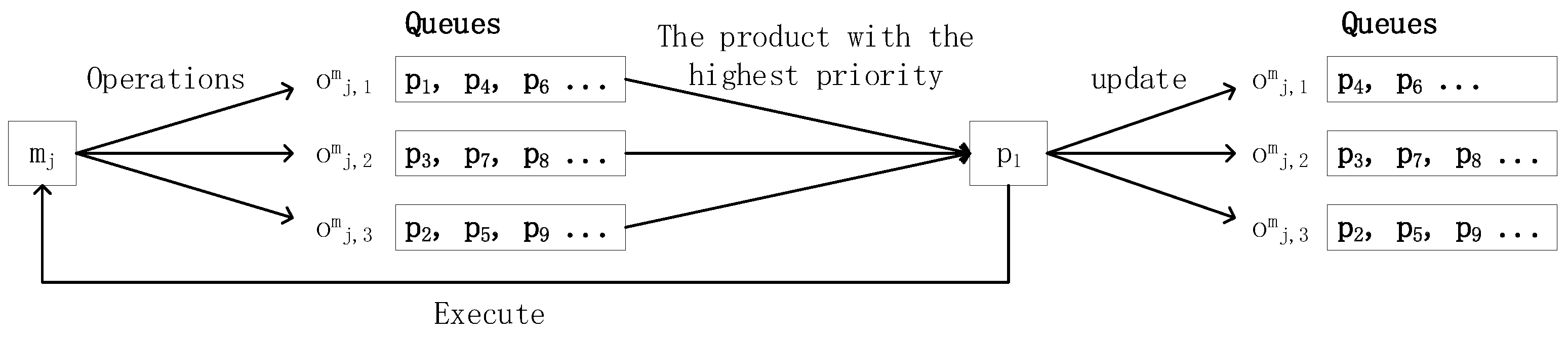
Based on the above analysis, the priority assignment algorithm is as shown in Algorithm 2. $\rho$ is the priority to be assigned currently, and $\overline{\rho }$ is the highest priority (line 1). Priorities are assigned in order of low to high (lines 1, 2, and 11). For each priority, the maximum production time ${\delta }_k$ for each product in P is calculated, as well as the remaining slack time $\widehat{{\delta }_k}$ before the order’s deadline, according to Equation (13) (lines 3–5). The larger the value of $\widehat{{\delta }_k}$, the sooner the product will be assigned. However, if the maximum $\widehat{{\delta }_k}$ is negative, it means that no product will be completed at the current priority. To minimize production cost, the product with the least cost loss will be assigned the current priority (lines 7–8). If the maximum $\widehat{{\delta }_k}$ is not negative, then $p_k$ can be produced, and the current priority $\rho$ is assigned to product $p_k$ (lines 9–10). Thereafter, the above steps are repeated for the next priority (line 11), until the priority assignment of all products is completed, and the function returns the assignment result (line 12). The time complexity of the algorithm is mainly in lines 2–5, with corresponding time complexities of $O\left(\right|P\left|\right)$, $O\left(\right|P\left|\right)$, $O\left(\right|O\left|\right)$, and $O\left(\right|Q\left|\right)$, respectively. Since the time complexities of lines 4 and 5 are both linear, the time complexity of Algorithm 2 is $O\left(n^3\right)$, which is smaller than that of Algorithm 1, which is $O\left(n^3\right)$.

5.3. Test Cases

A large number of test cases were randomly generated to evaluate the effectiveness and generalizability of the proposed algorithm. The parameter set of each test case is represented as <the maximum number of machines that can perform the same operation, the number of orders, the number of operations, the execution time interval of each operation, the deadline interval, the cost loss interval> (i.e., <$o,m,t,q,d,c$>). For example, the parameter set <$10,3,[1,10],5,[50,100],[1,100]$> means the job shop supports 10 operations, each operation can be executed by up to three machines, the time required for each operation is within [1, 10], there are currently five orders, and the deadlines of the orders are in the interval of [50, 100]. If an order cannot be delivered, its cost loss is in the interval of [1, 100].

The interval in the parameter set is used to reflect the diversity of test cases. When a test case is generated, a value in the corresponding interval is randomly selected as the order attribute, and a sudden breakdown of machines, operations, products, or orders is randomly placed to simulate dynamic events in actual production. To evaluate the generalizability of our proposed algorithm, for each parameter set, 1000 test cases are generated randomly, and then, the algorithm runs 1000 times to process them. We analyzed the effectiveness of the algorithm under different parameter configurations by sequentially changing each parameter.

5.4. Result Analysis

Z3 is the most widely used solver for OMT. However, its execution time is unacceptable for complex problems. In order for Z3 to solve the OMT formulation (Equations (1)–(12)), the parameter settings are <$3,2,[1,5],5,[10,20],\left[100\right]$>. For each parameter setting, 100 test cases were randomly generated. Since these test cases are simple, Z3 can finish in 10 min, and the proposed algorithm (denoted as SchPA) finishes in 2 ms. Compared with Z3, SchPA increases the cost by about 2%. However, when the number of orders is seven, Z3 cannot solve the test case in 2 h. To evaluate the generalizability of SchPA, in the following, we ignore Z3 and only compare SchPA with heuristic algorithms.

We compared SchPA with the First Come First Serve (FCFS) rule [35] and the shortest process time (SPT) rule [36]. FCFS is a simple rule in which the order that is placed first is produced first. SPT gives the highest priority to the job with the smallest operation time. In [37], the comparison between SPT and other classical methods was shown, and SPT has the most optimum outcome. This is why we chose SPT as a baseline method.

The algorithms in the present study were written in C++ and run on a Precision 5820 workstation. The solution time for all orders was less than 10 ms. The assessment index was the percentage of cost loss to the total cost of all orders. Cost loss was calculated using Equation (1), and total cost was obtained after the orders were generated. Each point in the following figure represents the average cost loss for 1000 random orders. For the purpose of comparison, the y-axis scale was kept constant at $[0,40\%]$.

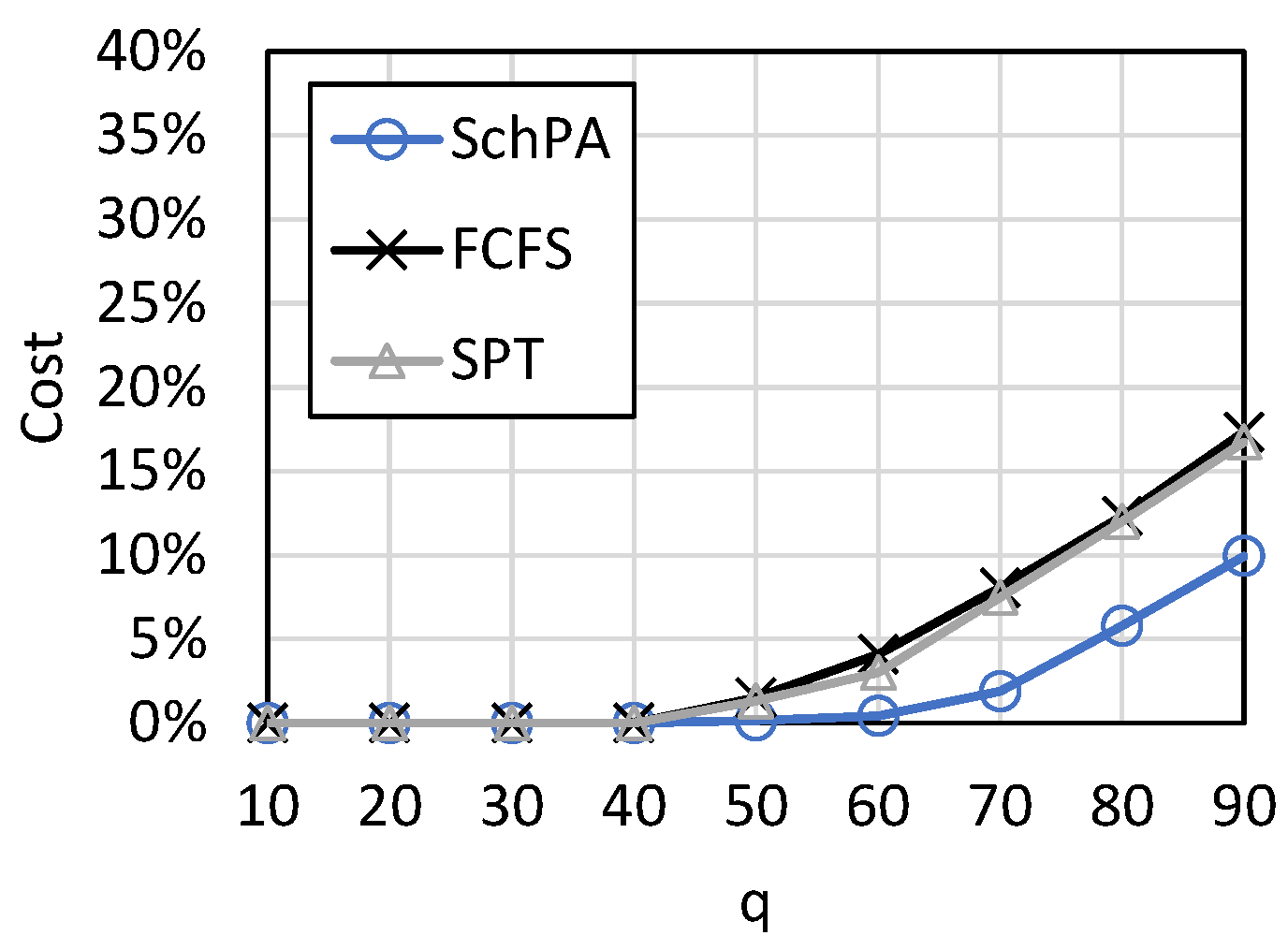
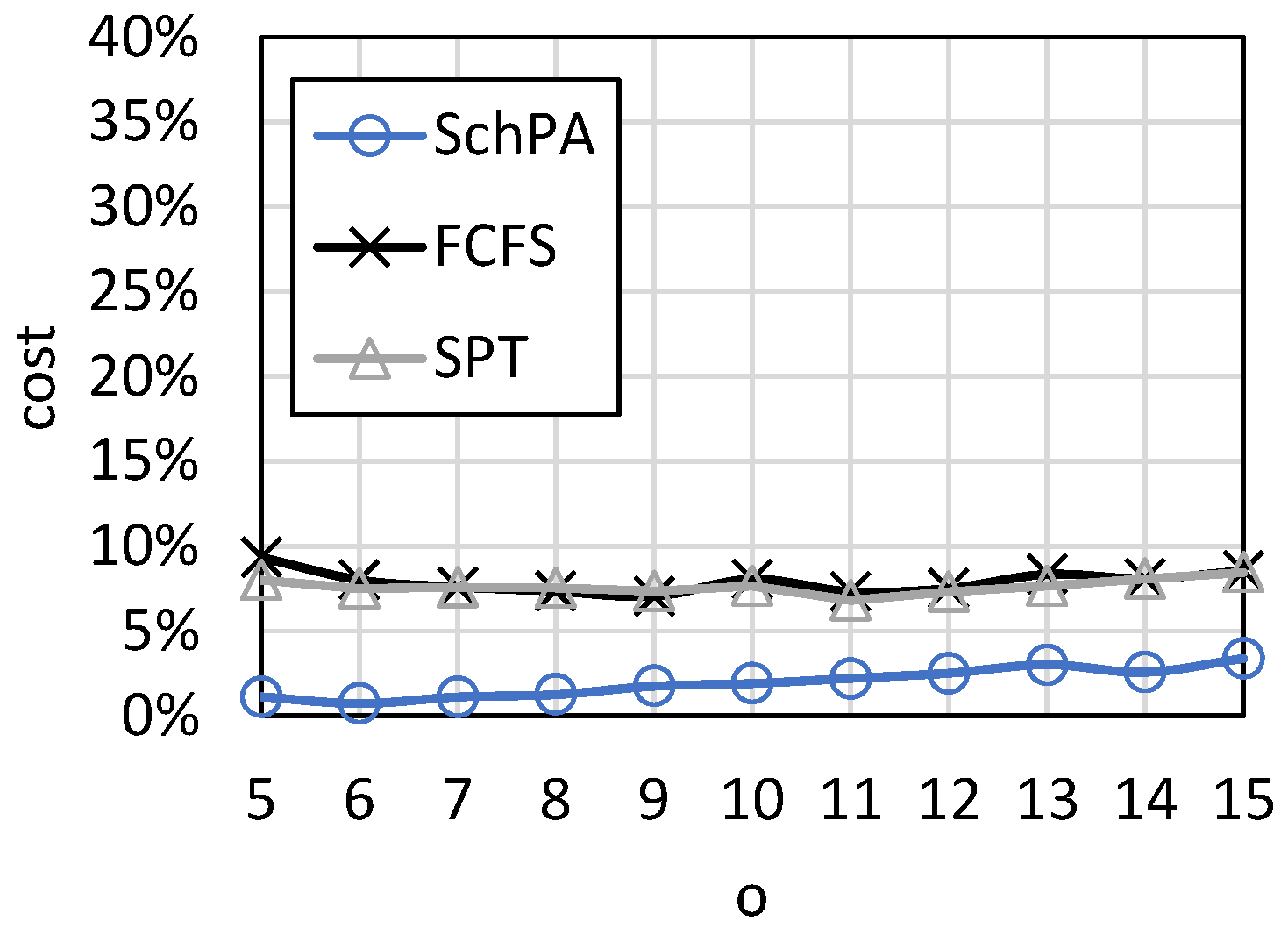
Figure 6 shows the cost loss curve with the number of orders. The parameter set is <10, 3, [1, 10], [10, 90], [50, 100], [1, 100]>. It can be seen that the cost loss increases with the number of orders. This is because the more orders there are, the more difficult it is for a limited number of machines to complete them. Since deadline and cost are optimized in our algorithm, it outperforms FCFS and SPT. SPT has less cost loss than FCFS because it can schedule production more efficiently. However, when an order fails, it needs to reproduce, so the cost loss is still large. When the number of orders is large, the proposed algorithm can reduce cost loss by about $6\%$. 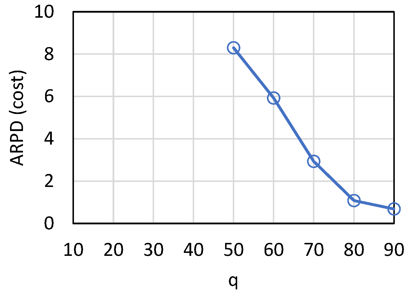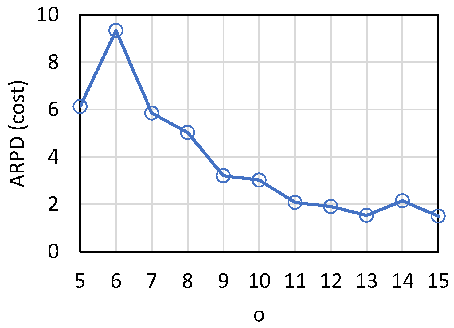To show the comparison result more clearly, the average relative percentage deviation (ARPD) of cost loss is shown in Figure 7. Since SPT had less cost loss than FCFS, we used SPT and SchPA to calculate the relative percentage deviation (RPD), i.e., RPD = (SPT − SchPA)/SchPA. ARPD was the average of RPD of the 1000 test cases. In the best case, the cost loss of SchPA is about one-ninth of SPT. 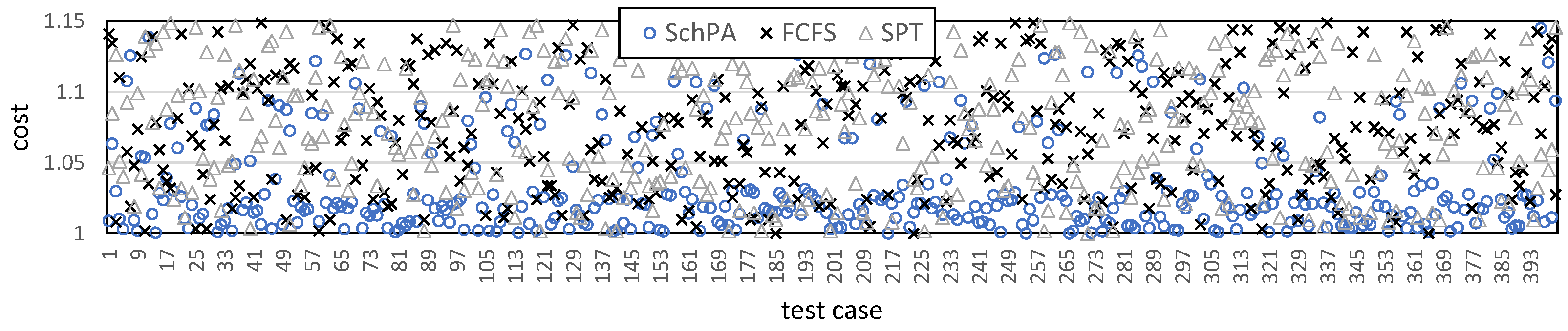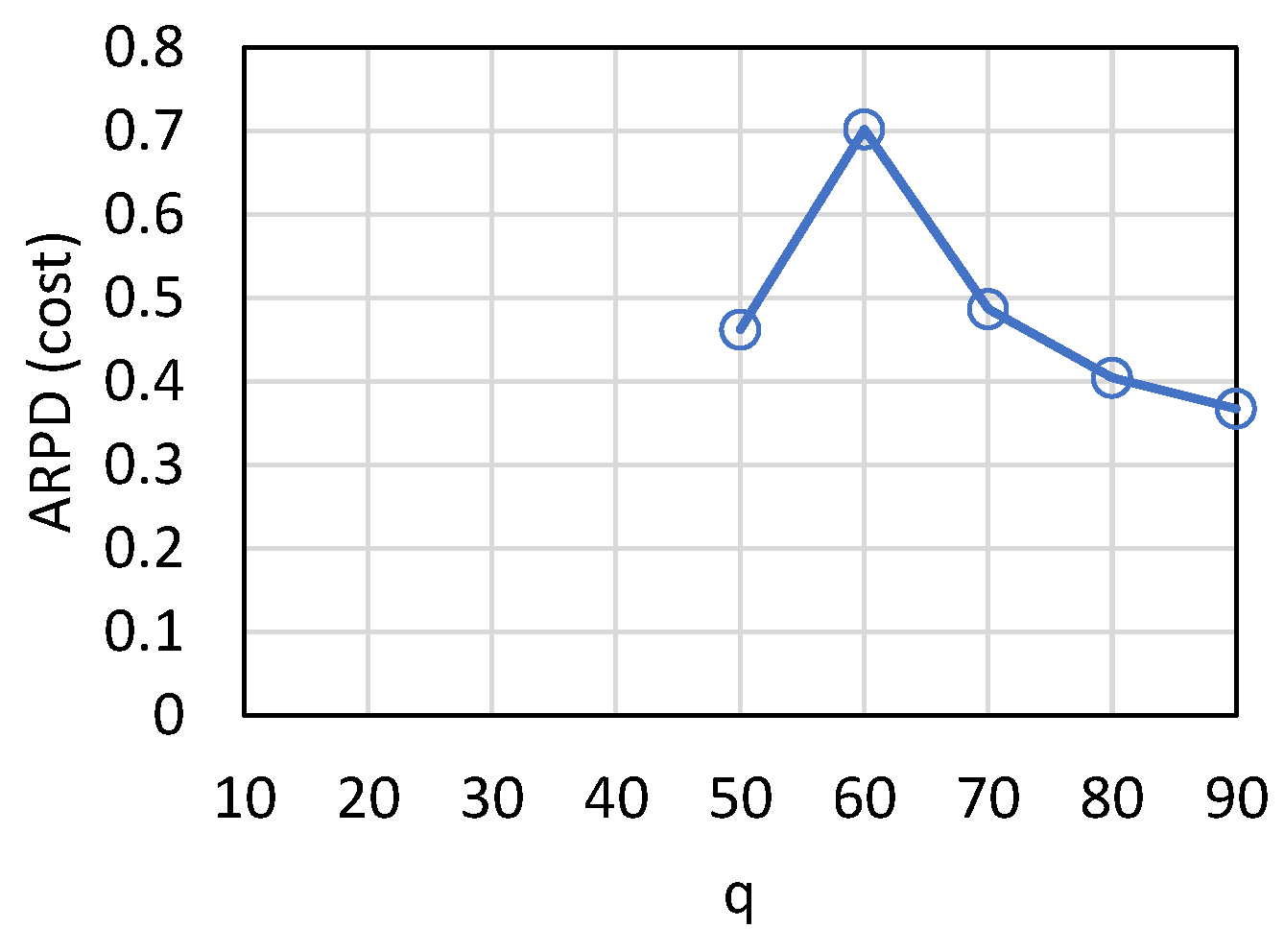Figure 8 shows the cost loss distribution when q = 70. Owing to the large number of orders, only partial results are shown. Regarding cost distribution, we can see that the proposed algorithm was below 1.04 for most of the orders.

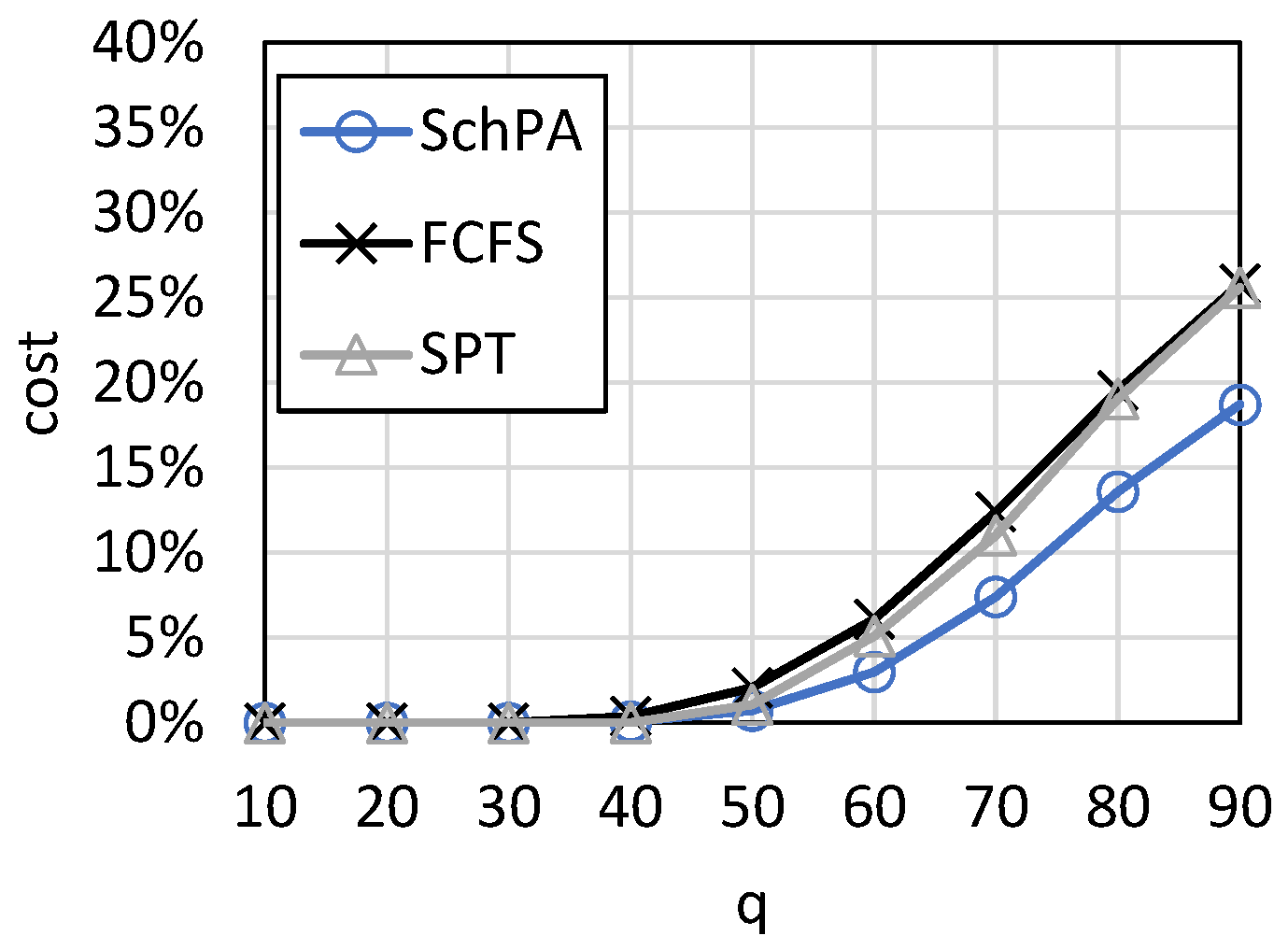
Figure 9 and Figure 10 show the cost loss and ARPD when the deadline is shortened from [50, 100] to [50, 80]. Comparing Figure 6 and Figure 9, we know that after the deadline is shortened, more orders cannot be completed in time. When there are 90 orders at the same time, the cost loss increases by about $10\%$. Therefore, if the deadline can be negotiated with the customer, the later the deadline, the better. If the deadline cannot be negotiated, loss can only be reduced by increasing the number of machines (Figure 11) or improving their efficiency (discussed later).

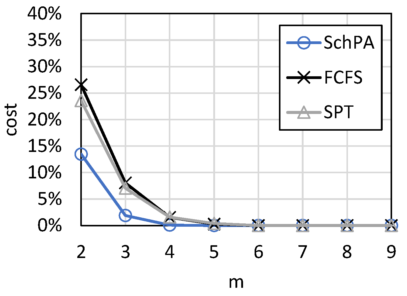
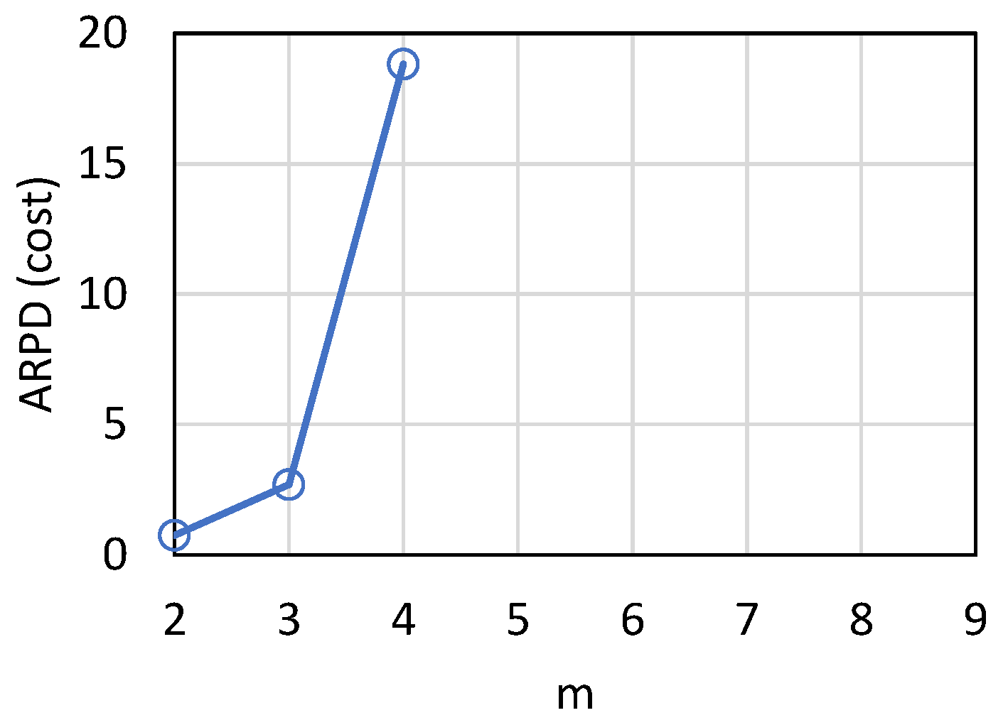
Figure 11 shows the variations in cost loss according to the number of machines, and Figure 12 shows ARPD for the test cases of Figure 12. The parameter set is <10, [2, 9], [1, 10], 70, [50, 100], [1, 100]>. It can be seen that when the number of machines increases to four, the cost loss decreases to zero. When the number of machines is small, the proposed algorithm is greatly superior to FCFS and SPT, suggesting that the proposed algorithm can precisely capture the competitive relationship between products and machines. When the number of machines is limited, the proposed algorithm should be used to reduce production losses.

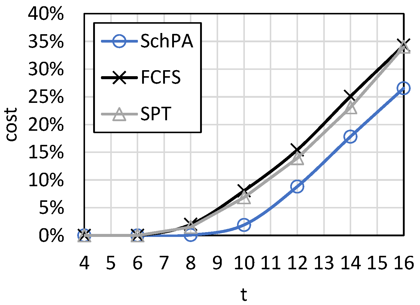
In Figure 13 and Figure 14, the execution time of each operation is modified. We can see that the shorter the execution time, the higher the machine efficiency. As can be seen, cost loss increases with a decrease in machine efficiency. If improving machine efficiency will increase the cost of other parts, it will be necessary to balance the costs of various parts, such that the system achieves optimal or near-optimal performance.

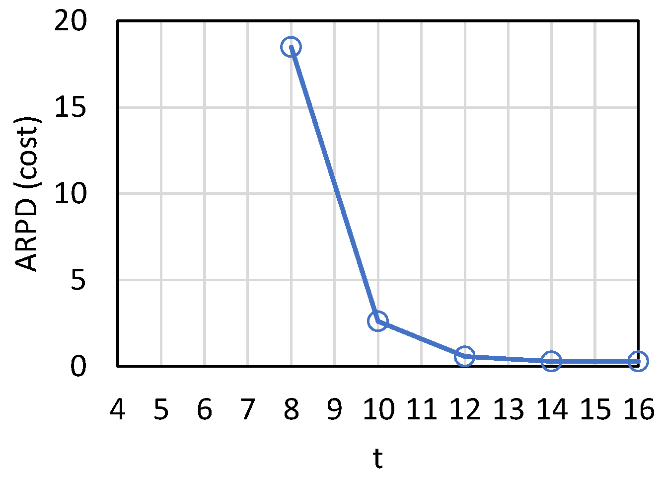
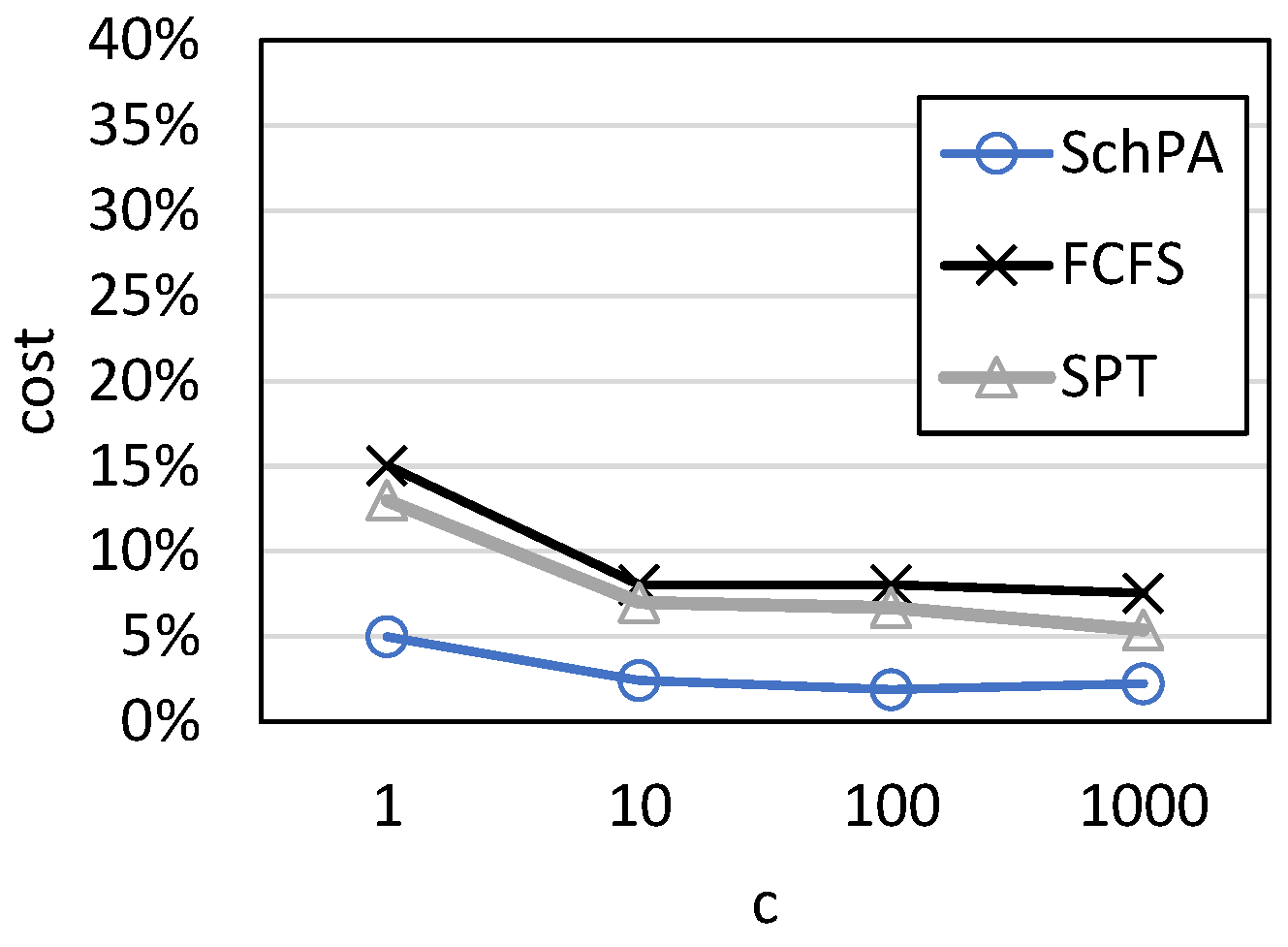
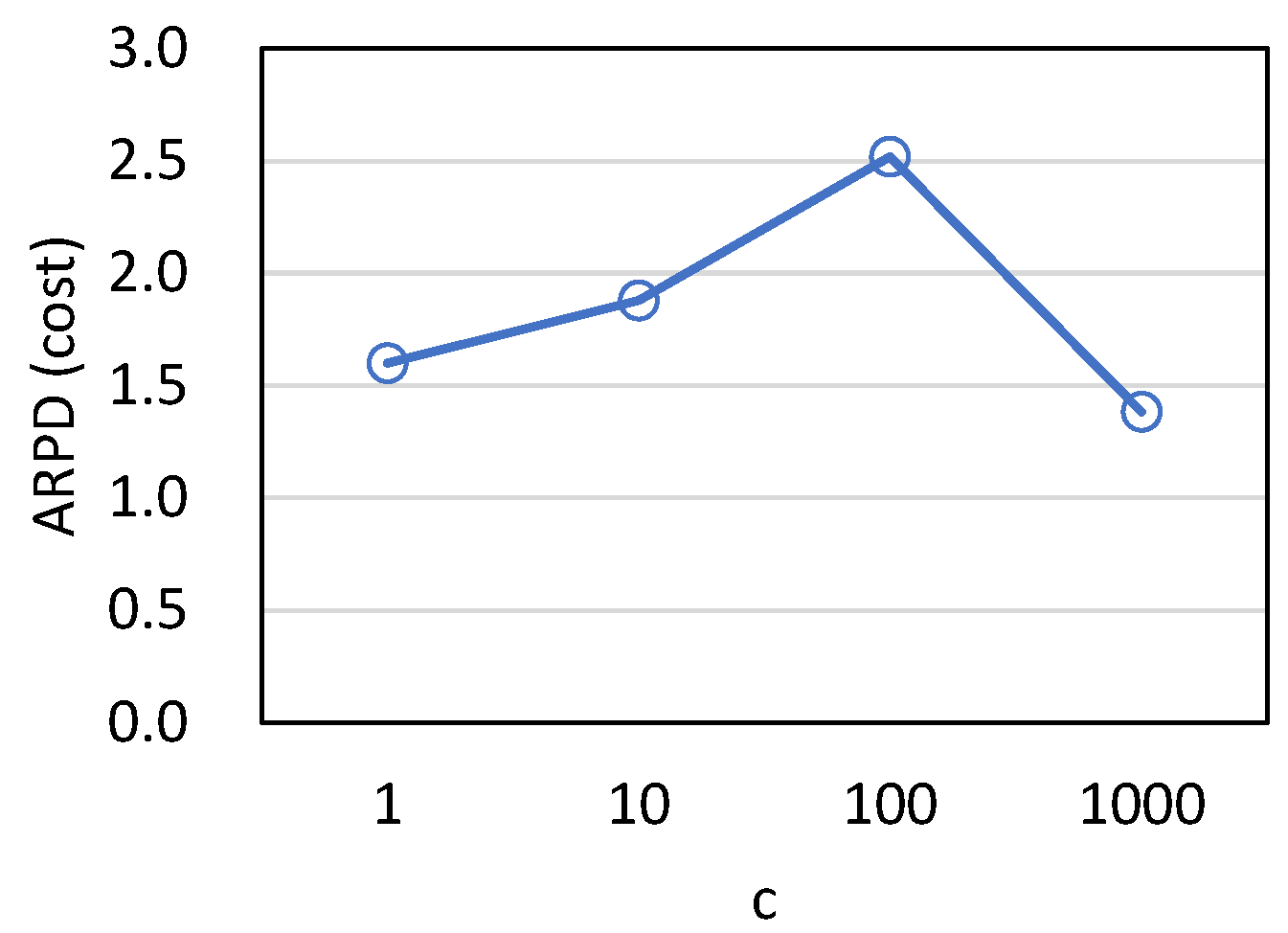
Figure 15 shows the variations in cost loss according to the number of operations, and Figure 16 is ARPD for the test cases of Figure 15. The parameter set is <[5, 15], 3, [1, 10], 70, [50, 100], [1, 100]>. As can be seen, the number of operations has little effect on cost loss. Figure 17 and Figure 18 show the results when the cost range is modified. We can see that the cost range has almost no effect on the percentage of loss, and loss is relatively high only when all products have the same cost. When the cost is randomly selected in the interval, it is not always the maximum value. Yet, when all products have the same cost, each product has the largest loss, resulting in a large loss. As long as the cost losses of different products are different, the percentage loss remains basically the same, regardless of the range of difference.

We also calculated the p-value results of a paired-sample t-test to distinguish SchPA and SPT. Among all these parameter sets, the largest p-value is $2.81\times {10}^{-6}$, which is smaller than 0.5. Therefore, SchPA significantly outperforms SPT.

6. Conclusions

In this study, we focused on the dynamic scheduling problem for flexible job shops with the goal of minimal cost loss. Although many relevant works have investigated the problem, most have limited dynamic support and cannot handle multiple dynamic events. We used a time-fine-grained model to describe the system state and proposed a priority scheduling algorithm based on completion time analysis. Since the model described the system state in a time-discrete manner and transformed the states at different times through our proposed efficient algorithm, this study can flexibly respond to multiple dynamic events.

To evaluate the effectiveness and generalizability of the proposed algorithm, we randomly generated extensive test cases and compared the proposed algorithm with FCFS and SPT. The results indicated that the proposed algorithm responded in milliseconds, and the cost optimization performance was superior to that of similar algorithms. Compared with FCFS and SPT, the proposed algorithm reduced cost loss by up to 11%.

In the future, we will consider the design of logistics systems in our problem. The logistics system supplies raw materials, components and integrated objects to production processes. Therefore, the stability and robustness of logistics systems are important to high-end manufacturing. In this paper, we assume that the logistics system is ideal and ignore its influence on production processes. In our next work, we will propose a holistic framework that supports the co-design of production and logistics management.