Quantized Fault-Tolerant Control for Descriptor Systems with Intermittent Actuator Faults, Randomly Occurring Sensor Non-Linearity, and Missing Data

Abstract

This paper examines the fault-tolerant control problem for discrete-time descriptor systems that are susceptible to intermittent actuator failures, nonlinear sensor data, and probability-based missing data. The discrete-time non-homogeneous Markov chain was adopted to describe the stochastic behavior of actuator faults. Moreover, Bernoulli-distributed stochastic variables with known conditional probabilities were employed to describe the practical features of random sensor non-linearity and missing data. In this study, the output signals were quantized and a dynamic output feedback controller was synthesized such that the closed-loop system was stochastically admissible and satisfied the strictly $(\mathbf{Q},\mathbf{S},\mathbf{R})$-$\gamma$-dissipative performance index. The theoretical developments are illustrated through numerical simulations of an infinite machine bus.

1. Introduction, Notations, and Outline

In this section, we provide the literature review and the notations and acronyms used in the present document, as well as the objectives and outline of this work.

1.1. Bibliographical Review

Singular systems, well known as descriptor systems, appear to be mathematical models that are able to depict the relationship between static and dynamic equations that simultaneously describe the behavior of different components in a system. Numerous applications of singular systems have been explored, including mechanical systems, robotics, chemical processes, and economical systems [1,2]. For digital control purposes, discrete-time singular systems have received great attention, with many publications in causality, asymptotic stability, and some prescribed performances [3,4,5,6,7].

Most dynamic systems, including actuators and sensors, are susceptible to unexpected faults or failures; in fact, many reasons may be responsible for a system’s instability and performance degradation. For specific reasons, one can cite sensors, actuators’ ages, sudden changes in working conditions, and internal components being corroded, among others, which could cause significant damage to the systems. Fault-tolerant control and fault diagnosis are crucial approaches for dynamic systems that seek to design satisfactory controllers to maintain the critical functionality of a system within admissible levels when suffering from faults or failures. Different elegant results have been developed to address the issue of reliable control for various classes of systems. Kavarian et al. develop a method for designing fault-tolerant controllers for power systems subject to random changes and actuator failures in [8]. The fault-tolerant control (FTC) method for wind-diesel hybrid systems with time-varying bounded sensor faults was proposed in [9]. In [10], the reliable observer-based control problem for discrete-time Takagi-Sugeno fuzzy systems with time-varying delays and stochastic actuator faults was formulated from the input-output approach. We also report on some results relating to fault-tolerant control for singular systems. For systems with actuator and/or sensor faults, sliding mode control was used [11]. The reliable control problem for nonlinear singularly perturbed systems with random actuator failures is discussed in [12]. Besides, as is mentioned in [13], the faults can be classified as permanent faults or intermittent faults. The first class of faults refers to faults that appear and are permanent and the last class of faults corresponds to the case where the faults occur occasionally and are limited in time. By virtue of its randomness, and intermittence, an intermittent fault needs a stochastic model to describe it [14,15]. In the meantime, Markovian jump systems have been proverbially regarded as a significant model for describing many systems with random structure changes [16,17,18]. Recently, the authors in [14] employed the Markov chain as a mathematical model to characterize the intermittent fault where the Markov chain was assumed to be homogeneous, with the probability of failure being independent of time. The hypothesis was, however, too restrictive in practice since the failure rate of any component usually depends on multiple aspects, for instance, its age and the extent of its solicitation. Thus, time-varying transition probabilities are more convenient, and the investigation of the non-homogeneous Markov process is more attractive, which is what motivated this study [19,20,21]. On the other hand, for most complex systems, the states are, however, not usually available for measurement and only a piece of partial information is accessible from the system outputs. A static/dynamic output feedback control design is often considered for such complex systems. In recent research, the dynamic output feedback control problem was also considered for singular systems [22,23,24]. Nevertheless, it should be pointed out that the output signals were generally taken from the sensors, which work practically under severe environments with aggressive conditions.Thus, it was necessary to pay close attention to the control problems for engineering systems with sensor non-linearities [4,11,25,26]. Moreover, it is understood that in engineering systems that employ digital channels for signal transmission, signal quantization becomes indispensable, especially when the bandwidth and energy are limited. Nevertheless, it may impact the system’s performance when signals are quantized. Thus, it is not surprising that researchers have recently investigated the problems of control and filtering using various quantization approaches [27,28]. For instance, in [29] the authors studied quantized non-stationary filtering for networked Markov switching repeated scalar non-linear systems. The work in [30], examined the quantification H_∞ control problem for non-linear stochastic network systems accompanied by probabilistic missing data. In [31], the authors studied the problem of event-triggered admissibilization for discrete-time singular Markovian jump network systems with delay and output quantizations. To the extent of our knowledge, few research efforts have been made on singular systems, and this established the second motivation for the present work.

1.2. Objective and Outline

This paper reveals the following significant contributions of our work: (1) the system under examination exhibited intermittent actuator faults, represented by a non-homogeneous Markov chain, and the data from different sensors might be missing and affected by stochastic nonlinearities; (2) sufficient conditions were established such that the closed-loop system was stochastically admissible under the strictly $(\mathbf{Q},\mathbf{S},\mathbf{R})$-$\gamma$-dissipative index; (3) a feasible control strategy was formulated for the considered control problem using the decoupling matrix procedure; and (4) simulation results of a physical plant to demonstrate the effectiveness of the control scheme was presented.

Table 1. Notations and acronyms used in the present document.

Symbol	Acronym/Notation
ℕ	the set of positive integer numbers
ℝ	the set of real numbers
$\mathcal{X}\in {ℝ}^n$	n-dimensional Euclidean space
$\mathit{X}\in {ℝ}^{n\times m}$	$n\times m$ real matrix
$\mathit{X}>0$	real symmetric positive definite matrix $\mathit{X}$
$\parallel \mathit{X}\parallel$	norm of the matrix $\mathit{X}$
${\mathit{X}}^{\top }$	transpose of the matrix $\mathit{X}$
$\mathrm{sym}\left(\mathit{X}\right)$	$\mathit{X}+{\mathit{X}}^{\top }$
$\lambda \left(\right)$	eigenvalue of a matrix
$\mathbb{E}$	mathematical expectation
*	term that is induced by symmetry
$r_k$	discrete-time Markov process
LMI	linear matrix inequalities
MJS	Markovian jump system
FTC	fault-tolerant control

displays the notations and acronyms that are used in this paper.

2. Preliminaries and Problem Statements

In this section, we introduce some preliminaries, which facilitate the comprehension of our proposal, and state the problem under study.

2.1. The Model

Consider a class of discrete-time descriptor systems described by the following state-space equations:

$$\left\{\begin{array}{cc}\hfill Ex(k+1)& =A\left(k\right)x\left(k\right)+B{u}_F\left(k\right)+B1w\left(k\right)\hfill \\ \hfill z\left(k\right)& =C1x\left(k\right)+D1w\left(k\right)\hfill \\ \hfill y\left(k\right)& =g\left(C2x\right(k\left)\right)\hfill \end{array}\right.$$

(1)

where $x\left(k\right){\in }^n$, $u_F\left(k\right){\in }^m$, and $w\left(k\right){\in }^w$ represent, respectively, the state vector, control input vector, and disturbance input vector, which lies in the square additive space $L_2[0,\infty )$. $z\left(k\right)\in p$ is the controlled output vector, and $y\left(k\right)\in n_y$ is the measurement output. The system is defined by the matrices E, B, $B_1$, $C_2$, $C1$, and $D_1$, which are assumed to be known, real, and constant with appropriate dimensions. The uncertain matrix $A\left(k\right)$ is defined as $A\left(k\right)=A+\Delta A\left(k\right)$, where A is a constant matrix, and $\Delta A\left(k\right)$ represents the parametric uncertainties.

2.2. Assumption

Throughout this paper, the following are assumed:

A1

$E\in {ℝ}^{n\times n}$ is a singular matrix such that $\left(E\right)=q<n$.

A2

Matrix $\Delta A$ is defined as $\Delta A=H\Delta \left(k\right)F$, where matrices H and F are known and constant with appropriate dimensions, and matrix $\Delta \left(k\right)$ is an unknown matrix verifying ${\Delta }^T\left(k\right)\Delta \left(k\right)\le I$.

A3

Due to actuator perturbation, we assume that there may exist an intermittent fault in the actuator, which is described as

$$\begin{array}{cc}\hfill & \begin{array}{cc}\hfill u_F\left(k\right)& ={\Theta }_{r\left(k\right)}u\left(k\right)\hfill \end{array}\hfill \end{array}$$

(2)

where matrix ${\Theta }_{r\left(k\right)}$ defines the actuator fault. For the sake of notation, in each $rk=i\in \mathbb{N}$, the related matrices or vectors to $rk$ are denoted using the index i.

Matrix ${\Theta }_i$ is defined as ${\Theta }_i=\overline{\theta }1i,\overline{\theta }2i,\cdots ,\overline{\theta }mi$, where the degradation levels of the actuator, $\theta si,s=1,2,\cdots m$, are defined in $\mathbb{N}$ with a probability matrix $\Pi \left(k\right)=\pi ij\left(k\right)$, $(i,j\in \mathbb{N})$. $\pi ij\left(k\right)$ defines the transition probability such that $\pi ij\left(k\right)=Pr\left(r\right(k+1)=j|r\left(k\right)=i)$, $\pi ij\left(k\right)\ge 0$ and ${\sum }_{j=1}^N\pi ij\left(k\right)=1$ for each i. A Markov chain that exhibits time-dependent transition probabilities is known as a non-homogeneous Markov chain. Transition matrix $\Pi \left(k\right)$ is assumed to have the following structure:

$$\begin{array}{c}\hfill \Pi \left(k\right)=\sum _{l=1}^M\alpha l\left(k\right){\Pi }^l\end{array}$$

(3)

where $0\le \alpha l\left(k\right)\le 1$ and ${\sum }_{l=1}^M\alpha l\left(k\right)=1$.

Accordingly, the time-varying transition probability matrix $\Pi \left(k\right)$ evolves on a polytope defined by its vertices ${\Pi }^l,l=1,\cdots ,M$, as well as referring to the polytopic time-varying transition matrix.

A4

Sensor outputs are sent over an unreliable network, where random non-linearities may affect the sensors. Here, we assume that the sensor output is as follows:

$$\begin{array}{c}\hfill \widehat{y}\left(k\right)=\theta \left(k\right)C2x\left(k\right)+(1-\theta \left(k\right))\phi \left(C2x\left(k\right)\right)\end{array}$$

(4)

where $\phi \left(C2x\right(k)$ is a non-linear function, which can be defined as

$$\begin{array}{c}\hfill \phi \left(C2x\right(k\left)\right)=L1C2x\left(k\right)+\varphi \left(C2x\right(k\left)\right)\end{array}$$

where $\varphi \left(C2x\right(k\left)\right)\in [L1,L2]$ is a nonlinear continuous function satisfying the sector condition [32,33]

$$\begin{array}{c}\hfill {\varphi }^T\left(C2x\left(k\right)\right)[\varphi \left(C2x\left(k\right)\right)-L\varphi \left(C2x\left(k\right)\right)]\le 0,\end{array}$$

(5)

where diagonal matrices $L1$ and $L2$ are known and verify $0\le L1<L2$ and $L=L2-L1$.

A5

Additionally, this study attempts to develop a controller using the quantization of sensor output. Based on the logarithmic quantizer, the following model can be used to define sensor output:

$$\begin{array}{c}\hfill q\left(\widehat{y}\left(k\right)\right)=\left[\begin{array}{cccc}q1\left({\widehat{y}}_1\left(k\right)\right)& q2\left({\widehat{y}}_2\left(k\right)\right)& \cdots & q{n}_y\left({\widehat{y}}_{n_y}\left(k\right)\right)\end{array}\right]\end{array}$$

(6)

where ${\widehat{y}}_s\left(k\right)$ is the ’s’th component of $\widehat{y}\left(k\right)$.

To define the logarithmic quantizer, we propose the following set of quantization levels:

$$\begin{array}{c}\hfill \mathcal{U}=\left\{u^l,u_i^l={\rho }^l{u}_0,l=0,\pm 1,\pm 2,\cdots \right\}\cup \left\{0\right\},u_0>0\end{array}$$

(7)

where ${\rho }^l$ is the quantization density verifying $0<{\rho }^l<1$.

Specifically, the corresponding logarithmic quantizer $q\left(\nu \right)$ is defined as follows:

$$q\left(\nu \right)=\left\{\begin{array}{cccc}\hfill & u^l\hfill & \hfill \mathrm{if}& \frac{1}{1+\delta }{\rho }^l{u}_0<\nu \le \frac{1}{1-\delta }{\rho }^l{u}_0\hfill \\ \hfill & 0\hfill & \hfill \mathrm{if}& \nu =0\hfill \\ \hfill & -q(-\nu )\hfill & \hfill \mathrm{if}& \nu <0\hfill \end{array}\right.$$

(8)

in which $\nu$ defines the input of the quantizer, and $\delta =\frac{1-\rho }{1+\rho }$.

The quantization error of a logarithmic quantizer is ${\Delta }_i=q_i\left({\nu }_i\right)-{\nu }_i$, where ${\Delta }_i\in [-\delta ,\delta ]$. Then, we have

$$\begin{array}{cc}\hfill q\left(\widehat{y}\left(k\right)\right)& =(I+\Delta q\left(k\right))\widehat{y}\left(k\right)\hfill \end{array}$$

where

$$\begin{array}{cc}\hfill \Delta q\left(k\right)& =diag\left({\Delta }_1,{\Delta }_2,\cdots {\Delta }_{n_y}\right)\hfill \end{array}$$

(9)

A6

The measured output suffers from both signal losses and quantization arriving to the controller, thus, the output is given by

$$\begin{array}{c}\hfill \begin{array}{cc}\hfill y\left(k\right)& =\beta \left(k\right)q\left(\widehat{y}\left(k\right)\right)=\beta \left(k\right)(I+\Delta q\left(k\right))\left(\theta \left(k\right)C2x\left(k\right)+(1-\theta (k\left)\right)\phi \left(C2x\right(k\left)\right)\right)\hfill \\ \hfill & =g\left(\right(C2x\left(k\right)\left)\right)\hfill \end{array}\end{array}$$

(10)

Stochastic parameters $\beta \left(k\right)$ and $\theta \left(k\right)$ in (4) and (10) are governed by the Bernoulli distribution so that we have the following:

$$\begin{array}{c}\hfill Pr\left(\tau \right(k)=1)=\tau ,Pr\left(\tau \right(k)=0)=1-\tau \end{array}$$

where $\tau \left(k\right)=\left\{\beta \right(k),\theta (k\left)\right\}$, $\tau =\{\beta ,\theta \}$, and $0\le \beta$, $\theta \le 1$ are known constants.

Let ${\rho }_1\left(k\right)=\beta \left(k\right)-\beta$ and ${\rho }_2\left(k\right)=\beta \left(k\right)\theta \left(k\right)-\beta \theta$. It can be seen that $\mathbb{E}\left\{{\rho }_l\left(k\right)\right\}=0$, $(l=1,2)$.

The purpose of this study was to design a mode-dependent full-order dynamic output controller of the following format:

$$\left\{\begin{array}{cc}\hfill E\widehat{x}(k+1)& ={\widehat{A}}_i\widehat{x}\left(k\right)+{\widehat{B}}_{i}y\left(k\right)\hfill \\ \hfill u\left(k\right)& ={\widehat{C}}_i\widehat{x}\left(k\right)\hfill \end{array}\right.$$

(11)

where ${\widehat{A}}_i$, ${\widehat{B}}_i$, and ${\widehat{C}}_i$ are the designed controller gains, and $\widehat{x}\left(k\right){\in }^n$ identifies the controller state. As a result of combining (1) and (11) we obtain the dynamics of a closed-loop system as follows:

$$\left\{\begin{array}{cc}\hfill \overline{E}\overline{x}(k+1)& =({\overline{A}}_i+\Delta \overline{A})\overline{x}\left(k\right)+B1w\left(k\right)+A\varphi i\varphi \left(C2x\left(k\right)\right)+{\rho }_1\left(k\right){{\rm Y}}_1\left(k\right)+{\rho }_2\left(k\right){{\rm Y}}_2\left(k\right)\hfill \\ \hfill z\left(k\right)& =C1\overline{x}\left(k\right)+D1w\left(k\right)\hfill \end{array}\right.$$

(12)

where ${\overline{x}}^T\left(k\right)={\left[\begin{array}{cc}{x}^T\left(k\right)& {\widehat{x}}^T\left(k\right)\end{array}\right]}^T$, $\overline{E}=(E,E)$, $\Delta \overline{A}\left(k\right)=\overline{H}\Delta \left(k\right)\overline{F}$, and

$$\begin{array}{cc}\hfill & {\overline{A}}_i={\overline{\mathbb{A}}}_i+{\overline{\mathbb{H}}}_i\Delta Q\left(k\right)\overline{\mathbb{F}},A\varphi i={\overline{\mathbb{A}}}_{\varphi i}+{\overline{\mathbb{H}}}_i\Delta Q\left(k\right)\overline{\mathbb{I}},\Delta Q\left(k\right)=(\Delta q\left(k\right),\Delta q\left(k\right))\hfill \\ \hfill {\overline{\mathbb{A}}}_i& =\left[\begin{array}{cc}A& B{\Theta }_i\widehat{}{C}_i\\ \beta \theta {\widehat{B}}_i{C}_2+\beta (1-\theta ){\widehat{B}}_{i}L1C_2& {\widehat{A}}_i\end{array}\right],{\overline{\mathbb{A}}}_{\varphi i}=\left[\begin{array}{c}0\\ \beta (1-\theta ){\widehat{B}}_i\end{array}\right]\hfill \\ \hfill B1& =\left[\begin{array}{c}{B}_1\\ 0\end{array}\right],{\overline{C}}_1=\left[\begin{array}{cc}{C}_1& 0\end{array}\right],D1=D1,{\overline{C}}_2=\left[\begin{array}{cc}{C}_2& 0\end{array}\right],\hfill \\ \hfill & \overline{H}=\left[\begin{array}{c}H\\ 0\end{array}\right],\overline{F}=\left[\begin{array}{cc}F& 0\end{array}\right],{\overline{\mathbb{H}}}_i=\left[\begin{array}{cc}0& 0\\ \beta \theta {\widehat{B}}_i& \beta (1-\theta ){\widehat{B}}_i\end{array}\right]\hfill \\ \hfill \overline{\mathbb{F}}& =\left[\begin{array}{cc}{C}_2& 0\\ L_1{C}_2& 0\end{array}\right],\overline{\mathbb{I}}=\left[\begin{array}{c}0\\ I\end{array}\right]\hfill \\ \hfill {{\rm Y}}_1\left(k\right)& =\left[\begin{array}{c}0\\ {\widehat{B}}_i\overline{\Delta }qL1C_{2}x\left(k\right)+{\widehat{B}}_i\overline{\Delta }q\varphi \left(C2x\left(k\right)\right)\end{array}\right],\overline{\Delta }q\left(k\right)=I+\Delta q\left(k\right)\hfill \\ \hfill {{\rm Y}}_2\left(k\right)& =\left[\begin{array}{c}0\\ {\widehat{B}}_i\overline{\Delta }q{C}_{2}x\left(k\right)-{\widehat{B}}_i\overline{\Delta }qL1C_{2}x\left(k\right)-{\widehat{B}}_i\overline{\Delta }q\varphi \left(C2x\left(k\right)\right)\end{array}\right]\hfill \end{array}$$

Remark 1

.

1.   As proposed in [34,35], expression (3) provides a non-homogeneous Markovian chain characterized by a time-varying transition probability, which may be described by a polytope with time-varying parameters. This case of Markovian chain degenerates the piecewise homogeneous and homogeneous cases.

2.   The Markov process is used here to model the actuator fault; hence, the precise transition probabilities were difficult to ascertain in practice. To circumvent this problem, time-varying transition probabilities were introduced in a convex polytopic set modeled by a non-homogeneous Markovian chain.

3.   From a practical point of view, the transition probability matrix can be be obtained using the method suggested in [36].

Before doing so, we recall, for nominal singular Markovian jump system (13), the subsequent definitions as follows:

$$\begin{array}{cc}\hfill Ex(k+1)& =A_{i}x\left(k\right)\hfill \end{array}$$

(13)

Definition 1

([37]).

1.   For each $i\in \mathbb{N}$, if $det(zE-A_i)$ is not identically zero, then pair $(E,A_i)$ is said to be regular;

2.   For each $i\in \mathbb{N}$, if $degdet(zE-A_i)=rank\left(E\right)$, then pair $(E,A_i)$ is said to be causal;

3.   If for any initial state $(r_0,x_0)$, $\mathbb{E}\left\{{\sum }_{k=0}^{\infty }{\parallel xk)\parallel }^2|r_0,x_0\right\}<\infty$ is verified, then system sys is stochastically stable;

4.   If system sys is regular, causal, and stochastically stable, then it is said to be stochastically admissible.

Throughout this study, we use a quadratic supply rate defined as

$$\begin{array}{c}\hfill J_{zw}\left(k\right)=z^T\left(k\right)\mathbf{Q}z\left(k\right)+2z^T\left(k\right)\mathbf{S}w\left(k\right)+w^T\left(k\right)\mathbf{R}w\left(k\right)\end{array}$$

where matrices $\mathbf{Q}$, $\mathbf{S}$, $\mathbf{R}$ are real, and $\mathbf{Q}={\mathbf{Q}}^T$, $\mathbf{R}={\mathbf{R}}^T$. We suppose that $\mathbf{Q}\le 0$ and $-\mathbf{Q}={\mathbf{Q}}_{-}^T{\mathbf{Q}}_{-}$.

Definition 2

([38]). System sys is strictly $(\mathbf{Q},\mathbf{S},\mathbf{R})$-γ dissipative for a given scalar γ, if the following inequality holds under zero initial condition:

$$\begin{array}{c}\hfill \begin{array}{cc}& s=0\infty J_{zw}\left(s\right)>\gamma s=0\infty w^T\left(s\right)w\left(s\right)\hfill \end{array}\end{array}$$

(14)

Remark 2.

The dissipativity criterion defined above unifies the performance and positive realness by an appropriate choice of different parameters. Actually, inequality (14) is equivalent to an performance index for $\gamma >0$ when $\mathbf{Q}$$=-I$, $\mathbf{S}$$=0$, and $\mathbf{R}$$=({\gamma }^2+\gamma )I$. The criterion corresponds to strict passivity or strictly positive realness if $\mathbf{Q}$$=0$, $\mathbf{S}$$=I$, and $\mathbf{R}$$=0$.

The following lemmas are introduced to help in the controller design process:

Lemma 1

([39]). Let $Q=Q^T$ and M and N be given matrices. For any matrix $F\left(k\right)$ satisfying $F^T\left(k\right)F\left(k\right)\le I$, $Q+MF\left(k\right)N+N^T{F}^T\left(k\right)M^T<0$ holds, if and only $Q+M{M}^T+N<0$ for any scalar $>0$.

Lemma 2.

If there exists a scalar α, matrices Q, N, M, U, and T satisfying

$$\begin{array}{c}\hfill \begin{array}{c}\hfill \left[\begin{array}{ccc}Q& M& \alpha N\\ & -\alpha \left(U\right)+T& 0\\ & *& -T\end{array}\right]<0\end{array}\end{array}$$

(15)

then,

$$\begin{array}{c}\hfill Q+\left(MU{N}^T\right)<0\end{array}$$

(16)

Proof. 

By checking the congruence transformation to (15) by ${[I,N{\left(U\right)}^{-T},N{\left(U\right)}^{-T}]}^T$, condition (16) holds. □

3. Admissibility and Dissipativity Analysis

This section shows the results on the stochastic mean square admissibility with dissipativity performance of the closed-loop system.

Theorem 1.

Given the scalars $\gamma >0$, ${\delta }_1,\cdots ,{\delta }_{n_y}$, and matrices $\mathbf{Q}$, $\mathbf{S}$, and $\mathbf{R}$, if there exist matrices $P_i^l>0$, $S_i$, $W_i$, ${\mathbb{V}}_{1i}$, ${\mathbb{V}}_{2i}$, and positive scalars $0i$, $1i$, $2i$ such that

$$\begin{array}{c}\hfill \left[\begin{array}{ccc}{\Xi }_i^{lq}({\overline{\mathbb{A}}}_i,{\overline{\mathbb{A}}}_{\varphi i})& {\mathbf{{\rm Y}}}_{1i}\Lambda & {\mathbf{{\rm Y}}}_2{W}_i\\ & -W_i& 0\\ & *& -W_i\end{array}\right]<0\end{array}$$

(17)

where

$$\begin{array}{cc}\hfill & \begin{array}{cc}\hfill & {\Xi }_i^{lq}({\overline{\mathbb{A}}}_i,{\overline{\mathbb{A}}}_{\varphi i})=\left[\begin{array}{cccccc}{\Xi }_{11i}^{lq}& {\Xi }_{12i}& {\Xi }_{13i}& {\Xi }_{14i}& C1i{\mathbf{Q}}_{-}& {\mathbb{V}}_{1i}H\\ & \Xi 22ilq& {\mathbb{V}}_{2i}{\overline{\mathbb{A}}}_{\varphi i}& {\mathbb{V}}_{2i}B1i& 0& {\mathbb{V}}_{2i}H\\ & *& -2_{1i}I& 0& 0& 0\\ & *& *& -{\Xi }_{44i}& D1i{\mathbf{Q}}_{-}& 0\\ & *& *& *& -I& 0\\ & *& *& *& *& {-}_{0i}I\end{array}\right]\hfill \end{array}\hfill \end{array}$$

(18)

$$\begin{array}{cc}\hfill & \begin{array}{cc}\hfill & {\mathbf{{\rm Y}}}_{1i}=\left\{{\mathbb{V}}_{1i}{\overline{\mathbb{H}}}_i,{\mathbb{V}}_{2i}{\overline{\mathbb{H}}}_i,0,0,0,0\right\},{\mathbf{{\rm Y}}}_2=\left\{{\overline{\mathbb{F}}}^T,0,{\overline{\mathbb{I}}}^T,0,0,0\right\}\hfill \\ \hfill & {\Xi }_{11i}^{lq}={\widehat{\Xi }}_{11i}^{lq}{+}_{0i}FF,{\widehat{\Xi }}_{11i}^{lq}=-{\overline{E}}^T(Pil-Xilq)\overline{E}+sym\left({\mathbb{V}}_{1i}({\overline{\mathbb{A}}}_i-\overline{E})\right)\hfill \\ \hfill & {\Xi }_{12i}={\left(Xilq\overline{E}\right)}^T+Si\overline{R}-{\mathbb{V}}_{1i}+{({\overline{\mathbb{A}}}_i-\overline{E})}^T{\mathbb{V}}_{2i}^T,\Xi 22ilq=-sym\left({\mathbb{V}}_{2i}\right)+Xilq\hfill \\ \hfill & {\Xi }_{13i}={\mathbb{V}}_{1i}{\overline{\mathbb{A}}}_{\varphi i}{+}_{1i}L{C}_2,{\Xi }_{14i}={\mathbb{V}}_{1i}B1i-C1i\mathbf{S}\hfill \\ \hfill & {\Xi }_{44i}=(\mathbf{R}-\gamma I)-\left(D1i\mathbf{S}\right),\Lambda =({\delta }_1,{\delta }_2,\cdots ,{\delta }_{n_y})\hfill \\ \hfill & Xilq=\sum _{j=1}^N\sum _{l=1}^M\sum _{q=1}^M\alpha l\left(k\right)\eta q\left(k\right)\pi ijlPjq,\alpha l(k+1)=\eta q\left(k\right)\hfill \end{array}\hfill \end{array}$$

(19)

then, closed-loop system CL is stochastically mean-square admissible with a strictly $(\mathbf{Q},\mathbf{S},\mathbf{R})$-γ-dissipative performance. $\overline{R}$ is a full column rank matrix such that $\overline{R}\overline{E}=0$ and $\left(\overline{R}\right)=2n-2r$.

Proof. 

Performing the Schur complement to (17), we get

$$\begin{array}{cc}\hfill {\Xi }_i^{lq}({\overline{\mathbb{A}}}_i,{\overline{\mathbb{A}}}_{\varphi i})& +{\mathbf{{\rm Y}}}_{1i}\Lambda W_i\Lambda {\mathbf{{\rm Y}}}_{1i}^T+{\mathbf{{\rm Y}}}_2{W}_i{\mathbf{{\rm Y}}}_2^T<0\hfill \end{array}$$

(20)

On the other hand, from the following inequality

$$\begin{array}{cc}\hfill 0& \le ({\mathbf{{\rm Y}}}_{1i}\Delta Q\left(k\right)W_i-{\mathbf{{\rm Y}}}_2)W_i^{-1}{({\mathbf{{\rm Y}}}_{1i}\Delta Q\left(k\right)W_i-{\mathbf{{\rm Y}}}_2)}^T\hfill \\ \hfill & ={\mathbf{{\rm Y}}}_{1i}\Delta Q\left(k\right)W_i\Delta Q\left(k\right){\mathbf{{\rm Y}}}_{1i}^T+{\mathbf{{\rm Y}}}_2{W}_i^{-1}{\mathbf{{\rm Y}}}_2^T-({\mathbf{{\rm Y}}}_1\Delta Q\left(k\right){\mathbf{{\rm Y}}}_2^T)\hfill \\ \hfill & \le {\mathbf{{\rm Y}}}_{1i}\Lambda W_i\Lambda {\mathbf{{\rm Y}}}_{1i}^T+{\mathbf{{\rm Y}}}_2{W}_i^{-1}{\mathbf{{\rm Y}}}_2^T-({\mathbf{{\rm Y}}}_1\Delta Q\left(k\right){\mathbf{{\rm Y}}}_2^T)\hfill \end{array}$$

we get

$$\begin{array}{cc}\hfill ({\mathbf{{\rm Y}}}_1\Delta Q\left(k\right){\mathbf{{\rm Y}}}_2^T)& \le {\mathbf{{\rm Y}}}_{1i}\Lambda W_i\Lambda {\mathbf{{\rm Y}}}_{1i}^T+{\mathbf{{\rm Y}}}_2{W}_i^{-1}{\mathbf{{\rm Y}}}_2^T\hfill \end{array}$$

(21)

Considering (9) with ${\Delta }_s\in [-{\delta }_s,{\delta }_s],s=1,2\cdots ,n_y$, results in

$$\begin{array}{cc}\hfill {\Xi }_i^{lq}({\overline{\mathbb{A}}}_i,{\overline{\mathbb{A}}}_{\varphi i})& +{\mathbf{{\rm Y}}}_{1i}{W}_i{\mathbf{{\rm Y}}}_{1i}^T+{\mathbf{{\rm Y}}}_1\Delta Q\left(k\right){\mathbf{{\rm Y}}}_2^T<0\hfill \end{array}$$

(22)

Using (21), it leads from (22) to

$$\begin{array}{c}\hfill {\Xi }_i^{lq}({\overline{\mathbb{A}}}_i,{\overline{\mathbb{A}}}_{\varphi i})+({\mathbf{{\rm Y}}}_{1i}\Delta Q\left(k\right){\mathbf{{\rm Y}}}_2^T)={\Xi }_i^{lq}({\overline{A}}_i,{\overline{A}}_{\varphi i})<0\end{array}$$

(23)

Assume $\Delta {\overline{A}}_{}=0$. We will firstly demonstrate that system CL is admissible. From th1con1, we have

$$\begin{array}{c}\hfill \Psi il=\left[\begin{array}{cc}-{\overline{E}}^T(Pil-Xilq)\overline{E}+sym\left({\mathbb{V}}_{1i}({\overline{A}}_i-\overline{E})\right)& {\left(Xilq\overline{E}\right)}^T+Si\overline{R}-{\mathbb{V}}_{1i}+{({\overline{A}}_i-\overline{E})}^{T}Wi\\ & -sym\left({\mathbb{V}}_{2i}\right)+Xilq\end{array}\right]<0\end{array}$$

(24)

Following this, we apply the congruence transformation to (24) by ${I,{(Ai-\overline{E})}^T}^T$, and we get

$$\begin{array}{c}\hfill {\overline{A}}_i^{T}Xilq{\overline{A}}_i-{\overline{E}}^{T}Pil\overline{E}+\left(Si\overline{R}Ai\right)<0\end{array}$$

(25)

For matrix $\overline{E}$, there exist two non-singular matrices $\widehat{M}$ and $\widehat{N}$ such that $\widehat{E}=\widehat{M}\overline{E}\widehat{N}=\left[\begin{array}{cc}I2r& 0\\ 0& 0\end{array}\right]$.

Define

$$\begin{array}{c}\hfill \begin{array}{cccc}\hfill Ai& =\widehat{M}{\overline{A}}_i\widehat{N}=\left[\begin{array}{cc}A11i& A12i\\ A21i& A22i\end{array}\right],\hfill & \hfill \widehat{R}& =\widehat{M}\overline{R}{\widehat{M}}^{-1}=\left[\begin{array}{cc}R11& R12\\ R21& R22\end{array}\right]\hfill \\ \hfill {\widehat{S}}_i& ={\widehat{M}}^{-T}{S}_i\widehat{N}=\left[\begin{array}{cc}S11i& S12i\\ S21i& S22i\end{array}\right],\hfill & \hfill {\widehat{P}}_i^l& ={\widehat{M}}^{-T}{P}_i^l{\widehat{M}}^{-1}=\left[\begin{array}{cc}P{11i}^l& P{12i}^l\\ & P{22i}^l\end{array}\right]\hfill \\ \hfill {\widehat{X}}_i^{lq}& ={\widehat{M}}^{-T}{X}_i^{lq}{\widehat{M}}^{-1}=\left[\begin{array}{cc}X{11i}^{lq}& X{12i}^{lq}\\ & X{22i}^{lq}\end{array}\right]\hfill \end{array}\end{array}$$

(26)

Using the fact that $\overline{R}\overline{E}=0$, it can be seen that ${\widehat{R}}_{}\widehat{E}=0$, $R11=0$ and $R21=0$.

Performing the congruence transformation to Inx1 by ${\widehat{N}}^T$ and $\widehat{N}$, respectively, the following inequality holds using (26):

$$\left[\begin{array}{cc}☆& ☆\\ ☆& sym(S12iR12iA22i+S22iR22iA22i+A12iX{12i}^{lq}A22i)+A12iX{12i}^{lq}A12i+A22iX{22i}^{lq}A22i\end{array}\right]<0$$

(27)

where ☆ represents the non concerned elements of the matrix. Thus, from (27), it can be verified that $sym(S12iR12iA22i+S22iR22iA22i+A12iX{12i}^{lq}A22i)<0$, which implies $A22i$ is nonsingular. By Definition 1, it can be concluded that pair $(\overline{E},{\overline{A}}_i)$ is regular and casual.

Our next step is to demonstrate that system (12) is stochastically stable. This can be accomplished by selecting a Lyapunov function which is defined as follows:

$$\begin{array}{c}\hfill V\left(k\right)={\overline{x}}^T\left(k\right){\overline{E}}^T\left(\sum _{l=1}^M\alpha l\left(k\right)Prkl\right)\overline{E}\overline{x}\left(k\right)\end{array}$$

(28)

Define $\Delta V\left(k\right)$ as the forward difference of $V\left(k\right)$. Therefore, along the trajectory of system (12), we can calculate

$$\begin{array}{c}\hfill \begin{array}{cc}\hfill \mathbb{E}\{\Delta V(k\left)\right\}& =\mathbb{E}\left\{V(k+1)-V\left(k\right)\left|x\right(k),rk=i\right\}\hfill \\ & ={\overline{x}}^T(k+1){\overline{E}}^T\left(\sum _{j=1}^N\sum _{l=1}^M\sum _{l=1}^M\alpha l\left(k\right)\alpha l(k+1)\pi ijlPjl\right)\overline{E}\overline{x}(k+1)\hfill \\ & -{\overline{x}}^T\left(k\right){\overline{E}}^T\left(\sum _{l=1}^M\alpha l\left(k\right)Pil\right)\overline{E}\overline{x}\left(k\right)\hfill \end{array}\end{array}$$

(29)

Note that ${\sum }_{l=1}^M\alpha l(k+1)Pjl={\sum }_{q=1}^M\eta q\left(k\right)Pjq$, where $0\le \eta q\left(k\right)\le 1$, and ${\sum }_{q=1}^M\eta q\left(k\right)=1$. Thus, we know that

$$\begin{array}{cc}\hfill & \begin{array}{cc}\hfill \mathbb{E}\{\Delta V(k\left)\right\}& ={\overline{x}}^T(k+1)\overline{E}\left(\sum _{j=1}^N\sum _{l=1}^M\sum _{q=1}^M\alpha l\left(k\right)\eta q\left(k\right)\pi ijlPjq\right)\overline{E}\overline{x}(k+1)\hfill \\ \hfill & -{\overline{x}}^T\left(k\right){\overline{E}}^T\left(\sum _{l=1}^M\alpha l\left(k\right)Pil\right)\overline{E}\overline{x}\left(k\right)\hfill \\ \hfill & ={\overline{x}}^T(k+1){\overline{E}}^{T}Xilq\overline{E}\overline{x}(k+1)-{\overline{x}}^T\left(k\right){\overline{E}}^T\left(\sum _{l=1}^M\alpha l\left(k\right)Pil\right)\overline{E}\overline{x}\left(k\right)\hfill \end{array}\hfill \end{array}$$

(30)

Let ${\overline{x}}_s\left(k\right)=\overline{x}(k+1)-\overline{x}\left(k\right)$. Equation (29) is equivalent to

$$\begin{array}{cc}\hfill \mathbb{E}\{\Delta V(k\left)\right\}& ={\overline{x}}_s^T\left(k\right)\overline{E}Xilq{\overline{E}}^T{\overline{x}}_s\left(k\right)-{\overline{x}}^T\left(k\right){\overline{E}}^T\left(\sum _{l=1}^M\alpha l\left(k\right)Pil-Xilq\right)\overline{E}\overline{x}\left(k\right)+2{\overline{x}}_s^T\left(k\right)\overline{E}Xilq{\overline{E}}^T\overline{x}\left(k\right)\hfill \end{array}$$

(31)

Additionally, using the fact that $\overline{R}\overline{E}=0$, we have

$$\begin{array}{c}\hfill 2\overline{x}kSi\overline{R}\overline{E}{\overline{x}}_s\left(k\right)=0\end{array}$$

(32)

Moreover, with appropriates matrices ${\mathbb{V}}_{1i}^T$ and ${\mathbb{V}}_{2i}^T$ it can be established from (12) that

$$\begin{array}{cc}\hfill & 2\mathbb{E}\left\{{\zeta }^T\left(k\right){\left[\begin{array}{ccc}{\mathbb{V}}_{1i}^T& {\mathbb{V}}_{2i}^T& 0\end{array}\right]}^T[-\overline{E}{\overline{x}}_s\left(k\right)+({\overline{A}}_i-\overline{E})\overline{x}\left(k\right)+A\varphi i\varphi \left(C2x\left(k\right)\right)+{\rho }_1\left(k\right){{\rm Y}}_1\left(k\right)+{\rho }_2\left(k\right){{\rm Y}}_2\left(k\right)]\right\}\hfill \\ \hfill & =2{\zeta }^T\left(k\right){\left[\begin{array}{ccc}{\mathbb{V}}_{1i}^T& {\mathbb{V}}_{2i}^T& 0\end{array}\right]}^T\left[\begin{array}{ccc}(Ai-\overline{E})& -I& A\varphi i\end{array}\right]\zeta \left(k\right)=0\hfill \end{array}$$

(33)

where $\zeta k=\left\{\overline{x}\left(k\right),\overline{E}{\overline{x}}_s\left(k\right),\varphi \left(C_{2}x\left(k\right)\right)\right\}$. According to sta cond, one has

$$\begin{array}{c}\hfill \begin{array}{c}\hfill -2_{1i}\left\{{\varphi }^T\left(C2x\left(k\right)\right)\left(\varphi \left(C2x\left(k\right)\right)-LC2\overline{x}\left(k\right)\right)\right\}\ge 0\end{array}\end{array}$$

(34)

where ${}_{1i}$ is a positive scalar.

Substituting Eq02–nonlincon4 into deltav1 gives us

$$\begin{array}{c}\hfill \mathbb{E}\{\Delta V\left(k\right)\}\le \zeta k{\overline{\Psi }}_i^{lq}\zeta k\end{array}$$

(35)

where

$$\begin{array}{c}\hfill {\overline{\Psi }}_i^{lq}=\left[\begin{array}{ccc}{\widehat{\Xi }}_{11i}^{lq}& {\Xi }_{12i}& {\Xi }_{13i}\\ & \Xi 22ilq& {\mathbb{V}}_{2i}A\varphi i\\ & *& -2_{1i}I\end{array}\right]\end{array}$$

(36)

From th1con1, we can deduce that ${\overline{\Psi }}_i^{lq}<0$, and del2 provides the following

$$\begin{array}{c}\hfill \begin{array}{c}\hfill \mathbb{E}\{\Delta V\left(k\right)\}\le \kappa {\zeta k}^2\end{array}\end{array}$$

(37)

where $\kappa <0$ is the largest eigenvalue of ${\overline{\Psi }}_i^{lq}$. Thus, from (37) we have

$$\begin{array}{cc}\hfill \mathbb{E}\{\sum _{l=0}^{\infty }{\parallel \zeta l\parallel }^2\}& \le {\displaystyle \frac{1}{\kappa }}\mathbb{E}\left\{\sum _{l=0}^{\infty }\Delta V\left(k\right)\right\}\hfill \end{array}$$

(38)

$$\begin{array}{cc}\hfill \mathbb{E}\{\sum _{l=0}^{\infty }{\parallel \zeta l\parallel }^2\}& \le -{\displaystyle \frac{1}{\kappa }}V\left(0\right)<\infty \hfill \end{array}$$

(39)

Thus, system CL is stochastically admissible according to Definition 1.

In order to show that system is $(\mathbf{Q},\mathbf{S},\mathbf{R})$-$\gamma$ dissipative, we present the following performance index:

$$\begin{array}{c}\hfill \begin{array}{cc}\hfill J_0& =\mathbb{E}\left\{k=0\infty (Jzw-\gamma w^T\left(k\right)w\left(k\right))\right\}\hfill \end{array}\end{array}$$

(40)

As with previous steps, the null equation

$$\begin{array}{c}\hfill 2{\psi }^T\left(k\right){\left[\begin{array}{cccc}{\mathbb{V}}_{1i}^T& {\mathbb{V}}_{2i}^T& 0& 0\end{array}\right]}^T\left[\begin{array}{cccc}(Ai-\overline{E})& -I& A\varphi i& B1i\end{array}\right]\psi \left(k\right)=0\end{array}$$

(41)

can be applied to get

$$\begin{array}{c}\hfill \mathbb{E}\{\Delta V\left(k\right)\}-Jzw\left(k\right)+\gamma w^T\left(k\right)w\left(k\right)={\psi }^T\left(k\right)\left({\overline{\Xi }}_i^{lq}\right)\psi \left(k\right)\end{array}$$

(42)

where $\psi \left(k\right)=\left\{\zeta \left(k\right),w\left(k\right)\right\}$, and

$$\begin{array}{cc}\hfill {\overline{\Xi }}_i^{lq}& =\left[\begin{array}{ccccc}{\widehat{\Xi }}_{11i}^{lq}& {\Xi }_{12i}& {\Xi }_{13i}& {\Xi }_{14i}& C1i{\mathbf{Q}}_{-}\\ & \Xi 22ilq& {\mathbb{V}}_{2i}{\overline{\mathbb{A}}}_{\varphi i}& {\mathbb{V}}_{2i}B1i& 0\\ & *& -2_{1i}I& 0& 0\\ & *& *& -{\Xi }_{44i}& D1i{\mathbf{Q}}_{-}\\ & *& *& *& -I\end{array}\right]\hfill \end{array}$$

(43)

According to th1con1, ${\overline{\Xi }}_i^{lq}<0$, and under zero initial conditions, we are left with the following equation:

$$\begin{array}{cc}\hfill J_0\le & k=0\infty \mathbb{E}\left\{\Delta V\left(k\right)-Jzw+\gamma w^T\left(k\right)w\left(k\right)\right\}\le \mathbb{E}\left\{V(\infty )+k=0\infty (-Jzw+\gamma w^T\left(k\right)w\left(k\right))\right\}<0\hfill \end{array}$$

(44)

Since $V(\infty )\ge 0$, it is easy to verify that $\mathbb{E}\left\{Jzw-\gamma w^T\left(k\right)w\left(k\right)\right\}>0$. Therefore, according to Definition 2, system CL is stochastically admissible and strictly $(\mathbf{Q},\mathbf{S},\mathbf{R})$-$\gamma$ dissipative.

Assume that $\Delta {\overline{A}}_{}\ne 0$. In the same manner as above, we arrive at

$$\begin{array}{c}\hfill {\overline{\Xi }}_i^{lq}+\left({\Gamma }_{1i}^T\Delta \left(k\right){\Gamma }_{2i}\right)<0\end{array}$$

(45)

where ${\Gamma }_{1i}=\left[\begin{array}{ccccc}{\left({\mathbb{V}}_{1i}H\right)}^T& {\left({\mathbb{V}}_{2i}H\right)}^T& 0& 0& 0\end{array}\right]$ and ${\Gamma }_{2i}=\left[\begin{array}{ccccc}\overline{F}& 0& 0& 0& 0\end{array}\right]$.

Because of ${\Delta }^T\left(k\right)\Delta \left(k\right)\le I$, inequality (22) holds according to Lemma 1. This ends the proof. □

Remark 3.

Theorem 1 establishes the existence of the controller such that the closed-loop system is stochastically admissible and strictly $(\mathbf{Q},\mathbf{S},\mathbf{R})$-γ dissipative. Due to the non-linear nature of the condition in the theorem, it cannot be solved with existing LMI solvers. The next section demonstrates the procedure to design the controller and overcome the BMI terms in (17).

4. Dissipativity Controller Design

In the sequel, the corresponding controller gains ${\widehat{A}}_i$, ${\widehat{B}}_i$, and ${\widehat{C}}_i$ will be designed based on the following conclusion.

Theorem 2.

System CL is stochastically admissible and strictly dissipative for a scalar $\gamma >0$, matrices $\mathbf{Q}$, $\mathbf{S}$, and $\mathbf{R}$, and tuning parameters $a1$, $a2$, $b1$, and $b2$, if the matrices $P_i^l>0$, $T_i>0$, $V_{1i}$, $V_{2i}$, $W_{1i}$, $W_{2i}$, $Y_i$, $W_i$, $U_i$, ${\widehat{\mathcal{A}}}_i$, ${\widehat{\mathcal{B}}}_i$, ${\widehat{\mathcal{C}}}_i$ and scalars $0i>0$, $1i>0$, and $2i>0$ exist such that the following LMI is true:

$$\begin{array}{c}\hfill \left[\begin{array}{ccccc}{\Psi }_i^{lq}({\mathcal{A}}_{1i},{\mathcal{A}}_{2i})& {\widetilde{\mathbf{{\rm Y}}}}_{1i}\Lambda & {\mathbf{{\rm Y}}}_{2i}{W}_i& {\widetilde{\mathbf{{\rm Y}}}}_{3i}& \alpha {\widetilde{\mathbf{{\rm Y}}}}_{4i}\\ & -W_i& 0& & \\ & *& -W_i& & \\ & *& & -\alpha \left(U_i\right)+T_i& 0\\ & *& & *& -T_i\end{array}\right]<0\end{array}$$

(46)

where

$$\begin{array}{cc}\hfill {\Psi }_i^{lq}({\mathcal{A}}_{1i},{\mathcal{A}}_{2i})& =\left[\begin{array}{cccccc}\Psi 11ilq& {\Psi }_{12i}& {\Psi }_{13i}{+}_{1i}L{C}_2& {\Psi }_{14i}-C1i\mathbf{S}& C1i{\mathbf{Q}}_{-}& {\Psi }_{16i}\\ & \Psi 22ilq& {\Psi }_{23i}& {\Psi }_{24i}& 0& {\Psi }_{26i}\\ & *& -2_{1i}I& 0& 0& 0\\ & *& *& -{\Phi }_{44i}& D1i{\mathbf{Q}}_{-}& 0\\ & *& *& *& -I& 0\\ & *& *& *& *& {-}_{0i}I\end{array}\right]\hfill \\ \hfill {\widetilde{\mathbf{{\rm Y}}}}_{1i}& =\left\{{\Psi }_{17i},{\Psi }_{27i},0,0,0,0\right\},\hfill \\ \hfill {\widetilde{\mathbf{{\rm Y}}}}_{3i}& =\left\{{\Psi }_{19i},{\Psi }_{29i},0,0,0,0,0,0\right\},\hfill \\ \hfill {\widetilde{\mathbf{{\rm Y}}}}_{4i}& =\left\{{\left[\begin{array}{cc}0& {\widehat{\mathcal{C}}}_i\end{array}\right]}^T,0,0,0,0,0,0,0\right\},\hfill \\ \hfill {\Psi }_{11i}^l& =-{\overline{E}}^T(Pil-Xilq)\overline{E}+sym\left({\mathcal{A}}_{1i}\right){+}_{0i}FF,\hfill \\ \hfill {\Psi }_{12i}& ={\left(Xilq\overline{E}\right)}^T+Si\overline{R}-{\mathbb{V}}_{1i}+{\left({\mathcal{A}}_{2i}\right)}^T,\hfill \\ \hfill \Psi 22ilq& =-sym\left({\mathbb{V}}_{2i}\right)+Xilq,\hfill \\ \hfill {\mathbb{V}}_{ji}& =\left[\begin{array}{cc}{V}_{ji}& a_j{Y}_i\\ W_{ji}& b_j{Y}_i\end{array}\right],j=1,2\hfill \\ \hfill {\mathcal{A}}_{ji}& =\left[\begin{array}{cc}{V}_{ji}(A-E)+a_j(\beta \theta {\widehat{\mathcal{B}}}_i{C}_2+\beta (1-\theta ){\widehat{\mathcal{B}}}_i{L}_1{C}_2)& a_j({\widehat{\mathcal{A}}}_i-Y_{i}E)+B{\Theta }_i{\widehat{\mathcal{C}}}_i\\ W_{ji}(A-E)+b_j(\beta \theta {\widehat{\mathcal{B}}}_i{C}_2+\beta (1-\theta ){\widehat{\mathcal{B}}}_i{L}_1{C}_2)& b_j({\mathcal{A}}_i-Y_{i}E)+B{\Theta }_i{\widehat{\mathcal{C}}}_i\end{array}\right],\hfill \\ \hfill {\Psi }_{j3i}& =\left[\begin{array}{c}{a}_j\beta (1-\theta ){\widehat{\mathcal{B}}}_i\\ b_j\beta (1-\theta ){\widehat{\mathcal{B}}}_i\end{array}\right]\hfill \\ \hfill {\Psi }_{j4i}& =\left[\begin{array}{c}{V}_{ji}{B}_1\\ W_{ji}{B}_1\end{array}\right],{\Psi }_{j6i}=\left[\begin{array}{c}{V}_{ji}H\\ W_{ji}H\end{array}\right],\hfill \\ \hfill {\Psi }_{j7i}& =\left[\begin{array}{cc}{a}_j\beta \theta {\widehat{B}}_i& a_j\beta (1-\theta ){\widehat{\mathcal{B}}}_i\\ b_j\beta \theta {\widehat{B}}_i& b_j\beta (1-\theta ){\widehat{\mathcal{B}}}_i\end{array}\right]\hfill \\ \hfill {\Psi }_{j9i}& =\left[\begin{array}{c}{V}_{ji}B{\Theta }_i-B{\Theta }_i{U}_i\\ W_{ji}B{\Theta }_i-B{\Theta }_i{U}_i\end{array}\right]\hfill \end{array}$$

(47)

Furthermore, the controller gains are given by

$$\begin{array}{c}\hfill \begin{array}{cccccc}\hfill Ai& =Y_i{\widehat{\mathcal{A}}}_i,\hfill & \hfill Bi& =Y_i{\widehat{\mathcal{B}}}_i,\hfill & \hfill Ci& =U_i{\widehat{\mathcal{C}}}_i\hfill \end{array}\end{array}$$

(48)

Proof. 

Based on Theorem 2, a feasible solution must satisfy the condition $-\left({\mathbb{V}}_{2i}\right)<0$ and $-\left(Ui\right)<0$. It follows that $Y_i$ and $U_i$ are nonsingular, and we get

$$\begin{array}{cccccc}\hfill {\widehat{\mathcal{A}}}_i& =Y_{i}Ai,\hfill & \hfill {\widehat{\mathcal{B}}}_i& =Y_{i}Bi,\hfill & \hfill {\widehat{\mathcal{C}}}_i& =U_{i}Ci\hfill \end{array}$$

(49)

According to Lemma 2, we obtain from (46)

$$\begin{array}{c}\hfill \left[\begin{array}{ccc}{\Psi }_i^{lq}({\mathcal{A}}_{1i},{\mathcal{A}}_{2i})& {\widetilde{\mathbf{{\rm Y}}}}_{1i}\Lambda & {\mathbf{{\rm Y}}}_{2i}{W}_i\\ & -W_i& 0\\ & *& -W_i\end{array}\right]+\left({\widetilde{\mathbf{{\rm Y}}}}_{3i}{U}_i{\widetilde{\mathbf{{\rm Y}}}}_{4i}^T\right)<0\end{array}$$

(50)

Note that $Ci=U_i{\widehat{\mathcal{C}}}_i$. Thus, it is easy to get

$$\begin{array}{c}\hfill {\widetilde{\mathbf{{\rm Y}}}}_{3i}{U}_i{\widetilde{\mathbf{{\rm Y}}}}_{4i}^T=\left[\begin{array}{cccccccc}\left[\begin{array}{cc}0& V_{1i}B{\Theta }_i{\widehat{C}}_i-B{\Theta }_i{\widehat{\mathcal{C}}}_i\\ 0& W_{1i}B{\Theta }_i{\widehat{C}}_i-B{\Theta }_i{\widehat{\mathcal{C}}}_i\end{array}\right]& 0& 0& 0& 0& 0& 0& 0\\ \left[\begin{array}{cc}0& V_{2i}B{\Theta }_i{\widehat{C}}_i-B{\Theta }_i{\widehat{\mathcal{C}}}_i\\ 0& W_{2i}B{\Theta }_i{\widehat{C}}_i-B{\Theta }_i{\widehat{\mathcal{C}}}_i\end{array}\right]& 0& 0& 0& 0& 0& 0& 0\\ 0& 0& 0& 0& 0& 0& 0& 0\\ 0& 0& 0& 0& 0& 0& 0& 0\\ 0& 0& 0& 0& 0& 0& 0& 0\\ 0& 0& 0& 0& 0& 0& 0& 0\\ 0& 0& 0& 0& 0& 0& 0& 0\\ 0& 0& 0& 0& 0& 0& 0& 0\end{array}\right]\end{array}$$

(51)

Using (51), inequality (50) is equivalent to

$$\begin{array}{c}\hfill \left[\begin{array}{ccc}{\Psi }_i^{lq}({\mathbf{A}}_{1i},{\mathbf{A}}_{2i})& {\widetilde{\mathbf{{\rm Y}}}}_{1i}\Lambda & {\mathbf{{\rm Y}}}_{2i}{W}_i\\ & -W_i& 0\\ & *& -W_i\end{array}\right]<0\end{array}$$

(52)

where

$$\begin{array}{cc}\hfill {\mathbf{A}}_{1i}& ={\mathcal{A}}_{1i}+\left[\begin{array}{cc}0& V_{1i}B{\Theta }_i{\widehat{C}}_i-B{\Theta }_i{\widehat{\mathcal{C}}}_i\\ 0& W_{1i}B{\Theta }_i{\widehat{C}}_i-B{\Theta }_i{\widehat{\mathcal{C}}}_i\end{array}\right]={\mathbb{V}}_{1i}({\overline{\mathbb{A}}}_i-\overline{E})\hfill \\ \hfill {\mathbf{A}}_{2i}& ={\mathcal{A}}_{2i}+\left[\begin{array}{cc}0& V_{2i}B{\Theta }_i{\widehat{C}}_i-B{\Theta }_i{\widehat{\mathcal{C}}}_i\\ 0& W_{2i}B{\Theta }_i{\widehat{C}}_i-B{\Theta }_i{\widehat{\mathcal{C}}}_i\end{array}\right]={\mathbb{V}}_{2i}({\overline{\mathbb{A}}}_i-\overline{E})\hfill \\ \hfill {\mathbb{V}}_{1i}& =\left[\begin{array}{cc}{V}_{1i}& a_1{Y}_i\\ W_{1i}& b_1{Y}_i\end{array}\right],{\mathbb{V}}_{2i}=\left[\begin{array}{cc}{V}_{2i}& a_2{Y}_i\\ W_{2i}& b_2{Y}_i\end{array}\right]\hfill \end{array}$$

Moreover, using the fact that

$$\begin{array}{cc}\hfill & {\Psi }_{j3i}={\mathbb{V}}_{ji}{\overline{\mathbb{A}}}_{\varphi i},{\Psi }_{j4i}={\mathbb{V}}_{ji}B1i,{\Psi }_{j7i}={\mathbb{V}}_{ji}{\overline{\mathbb{H}}}_i,j=1,2\hfill \end{array}$$

it can be verified that (52) is equivalent to (17). Hence, according to Theorem 1, if (46) holds then system CL is stochastically admissible and strictly dissipative. □

Remark 4.

In comparison with existing results in [23,40,41], the proposed control design scheme’s main benefit is its simplicity and lesser conservativeness. In [40], the SVD decomposition technique was applied with a specific structure of auxiliary matrices. Our proposed methodology differed from the one in [23] since it is valid only for systems with measurable states and requires the tuning of many scalars. Additionally, contrary to our study [41], some scalars were introduced in the matrix ${\mathbb{V}}_{1i}$ and ${\mathbb{V}}_{2i}$ in order to reduce the conservatism of the method.

5. A Numerical Application

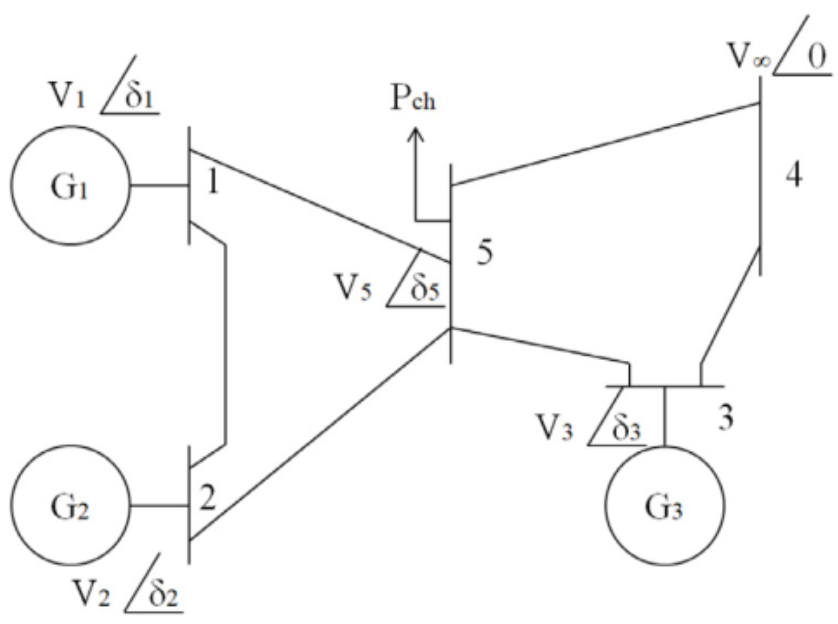
5.1. A Machine Infinite-Bus System

With the help of the example of a machine infinite-bus system displayed in Figure 1, and borrowed from [42], we demonstrate both the efficiency and correctness of the proposed control scheme.

From the publication [43], the following model describes the corresponding simulation system:

$$\begin{array}{c}\hfill \begin{array}{cc}\hfill A& =\left[\begin{array}{ccccccc}1& 0& 0& 0.01& 0& 0& 0\\ 0& 1& 0& 0& 0.01& 0& 0\\ 0& 0& 1& 0& 0& 0.01& 0\\ -1.0714& 0.7143& 0& 0.9593& 0& 0& 0.3571\\ 0.3846& -0.8461& 0& 0& 0.9423& 0& 0.4615\\ 0& 0& -0.75& 0& 0& 0.945& 0.4\\ 0.005& 0.012& 0.008& 0& 0& 0& -0.035\end{array}\right],\hfill \\ \hfill B& =\left[\begin{array}{ccc}0& 0& 0\\ 0& 0& 0\\ 0& 0& 0\\ 0.7142& 0& 0\\ 0& 0.3846& 0\\ 0& 0& 0.5\\ 0& 0& 0\end{array}\right],B_1=\left[\begin{array}{c}0\\ 0\\ 0\\ 0\\ 0\\ 0\\ 0.01\end{array}\right]C_2=\left[\begin{array}{ccccccc}1& 0& 0& 0& 0& 0& 0\\ 0& 1& 0& 0& 0& 0& 0\\ 0& 0& 1& 0& 0& 0& 0\\ 0& 0& 0& 0& 0& 0& 1\end{array}\right],\hfill \end{array}\end{array}$$

and $E=(1,1,1,1,1,1,0)$. The other parameters are respectively selected as follows:

$$\begin{array}{c}\hfill \begin{array}{cc}& \left[\begin{array}{c}H\\ \\ F\\ \\ C11\\ \\ D1\end{array}\right]=\left[\begin{array}{c}{\left[\begin{array}{ccccccc}0& 0& 0& 0.01& 0.01& 0.01& 0.01\end{array}\right]}^T\\ \\ \left[\begin{array}{ccccccc}0.1& -0.1& 0.1& 0& 0& 0& -0.1\end{array}\right]\\ \\ \left[\begin{array}{ccccccc}0.1& 0.1& 0.1& 0& 0& 0& 0.1\end{array}\right]\\ \\ 0\end{array}\right]\hfill \end{array}\end{array}$$

We suppose that an intermittent actuator fault may occur randomly according to a time-varying Markov chain with fault matrices selected as ${\Theta }_1=(1,1,1)$, and ${\Theta }_2=(0.5,0.5,0.5)$, and a transition probability defined by the following vertices:

$$\begin{array}{cccccc}\hfill {\Pi }^1& =\left[\begin{array}{cc}0.5& 0.5\\ 5/14& 9/14\end{array}\right],\hfill & \hfill {\Pi }^2& =\left[\begin{array}{cc}0.7& 0.3\\ 0.6& 0.4\end{array}\right],\hfill & \hfill {\Pi }^3& =\left[\begin{array}{cc}0.75& 0.25\\ 0.65& 0.35\end{array}\right],\hfill \end{array}$$

Moreover, the following non linear function

$$\begin{array}{c}\hfill \phi \left(C2x\left(k\right)\right)={\displaystyle \frac{L1+L2}{2}}C2x\left(k\right))+{\displaystyle \frac{L2-L1}{2}}sin\left(C2x\left(k\right)\right)\end{array}$$

is borrowed to represent the sensor non-linearity with $L_1=(0.5,0.5,0.5,0.5)$ and $L_2=(0.8,0.8,0.8,0.8)$. The parameters of the logarithmic quantizer are selected as $u_0=0.1$ and $\rho =0.9$. Let $\mathbf{Q}=-0.1,\mathbf{S}=0.1,\mathbf{R}=10$, $\gamma =0.1$, $R_0=\left[\begin{array}{cc}{0}_{7,6}& I_{7,1}\end{array}\right]$, $\overline{R}=(R_0,R_0)$, $a_1=1$, $b_1=0$, $a_2=1$, $b_2=0$, $\alpha =0.1$, ${}_0=1$, and ${}_1=1$.

A viable solution is found using Yalmip’s toolbox in conjunction with Mosek’s solver at $\beta =0.9$, $\theta =0.8$, and

$$\begin{array}{c}\hfill \begin{array}{cc}\hfill {\widehat{A}}_1& =\left[\begin{array}{ccccccc}0.65823& 0.0004064& 0.001535& 0.013364& 0.000794& 0.0061627& -0.0025474\\ 0.0047828& 0.66035& 0.0028214& 0.017249& 0.016817& 0.0067394& -0.0020184\\ 0.0023727& 0.0023443& 0.65729& 0.0074535& 0.0030585& 0.0075329& -0.0015125\\ -0.001726& -0.042823& -0.0083913& 0.59108& -0.036362& -0.023284& -0.0025816\\ 0.035663& 0.0067386& 0.0093891& -0.048313& 0.61179& -0.011463& -0.0015296\\ -0.010618& -0.017083& 0.020782& -0.014012& -0.011638& 0.6231& -0.0011323\\ 0.003645& 0.0030258& 0.00222& 0.0017253& -0.0011264& 0.00022401& -0.49802\end{array}\right]\hfill \\ \hfill {\widehat{B}}_1& =\left[\begin{array}{cccc}-0.05209& 0.013598& -0.0007033& 0.047023\\ 0.015709& -0.062511& 0.0060032& 0.047707\\ -0.0024841& 0.0037372& -0.058534& 0.032604\\ 0.19178& -0.017745& 0.0011332& -0.16227\\ 0.026467& 0.15574& -0.0050712& -0.16976\\ 0.026843& -0.0054818& 0.16765& -0.1031\\ -0.0014821& -0.0058124& -0.0033069& 0.010051\end{array}\right]\hfill \\ \hfill {\widehat{C}}_1& =\left[\begin{array}{ccccccc}-0.0256& 0.039964& 0.019995& 0.016935& -0.077525& -0.038215& -8.7587e-05\\ -0.056836& -0.082333& -0.013872& 0.083229& 0.13775& 0.0011287& 9.8431e-05\\ 0.026176& 0.023931& -0.11231& -0.11& -0.086408& 0.14403& -1.9844e-05\end{array}\right]\hfill \\ \hfill {\widehat{A}}_2& =\left[\begin{array}{ccccccc}0.65804& 0.00034327& 0.0013678& 0.0039296& 0.0007452& 0.0013286& -0.0017139\\ 0.0027157& 0.65996& 0.0017229& 0.0081953& 0.0060933& 0.0016663& -0.0014004\\ 0.0015253& 0.0015426& 0.65774& 0.00092097& 0.00060671& 0.0040795& -0.00092355\\ 0.018616& -0.021029& -0.002425& 0.64437& -0.0028923& 4.4378e-05& -0.0010219\\ 0.013199& 0.021075& -0.0037748& -0.013745& 0.64909& 0.0026206& -0.00024366\\ -0.0044677& -0.0065649& 0.030394& 0.0021783& 0.0034892& 0.6412& -0.0002276\\ 0.0022379& 0.0022817& 0.0014652& 0.00017662& -0.0012586& -0.0005046& -0.49805\end{array}\right]\hfill \\ \hfill {\widehat{B}}_2& =\left[\begin{array}{cccc}-0.061413& 0.017146& 0.0064549& 0.046044\\ 0.013098& -0.063389& 0.0080104& 0.048076\\ 0.0036008& 0.0070987& -0.071588& 0.028373\\ 0.11256& -0.022614& -0.011207& -0.077291\\ 0.0031899& 0.10688& -0.016069& -0.096737\\ -0.002898& -0.009896& 0.13612& -0.055888\\ -0.0019342& -0.0064795& -0.0036871& 0.011058\end{array}\right]\hfill \\ \hfill {\widehat{C}}_2& =\left[\begin{array}{ccccccc}-0.1033& 0.076039& 0.016612& 0.062354& -0.087665& -0.032075& -3.8798e-05\\ -0.038447& -0.17818& 0.020649& 0.027777& 0.12359& -0.042474& -3.3119e-05\\ 0.03359& 0.030564& -0.21223& -0.076694& -0.065088& 0.19051& -7.1046e-06\end{array}\right].\hfill \end{array}\end{array}$$

The control scheme proposed in [41] is not feasible with the above parameters for this system, which indicates the superiority of the new strategy.

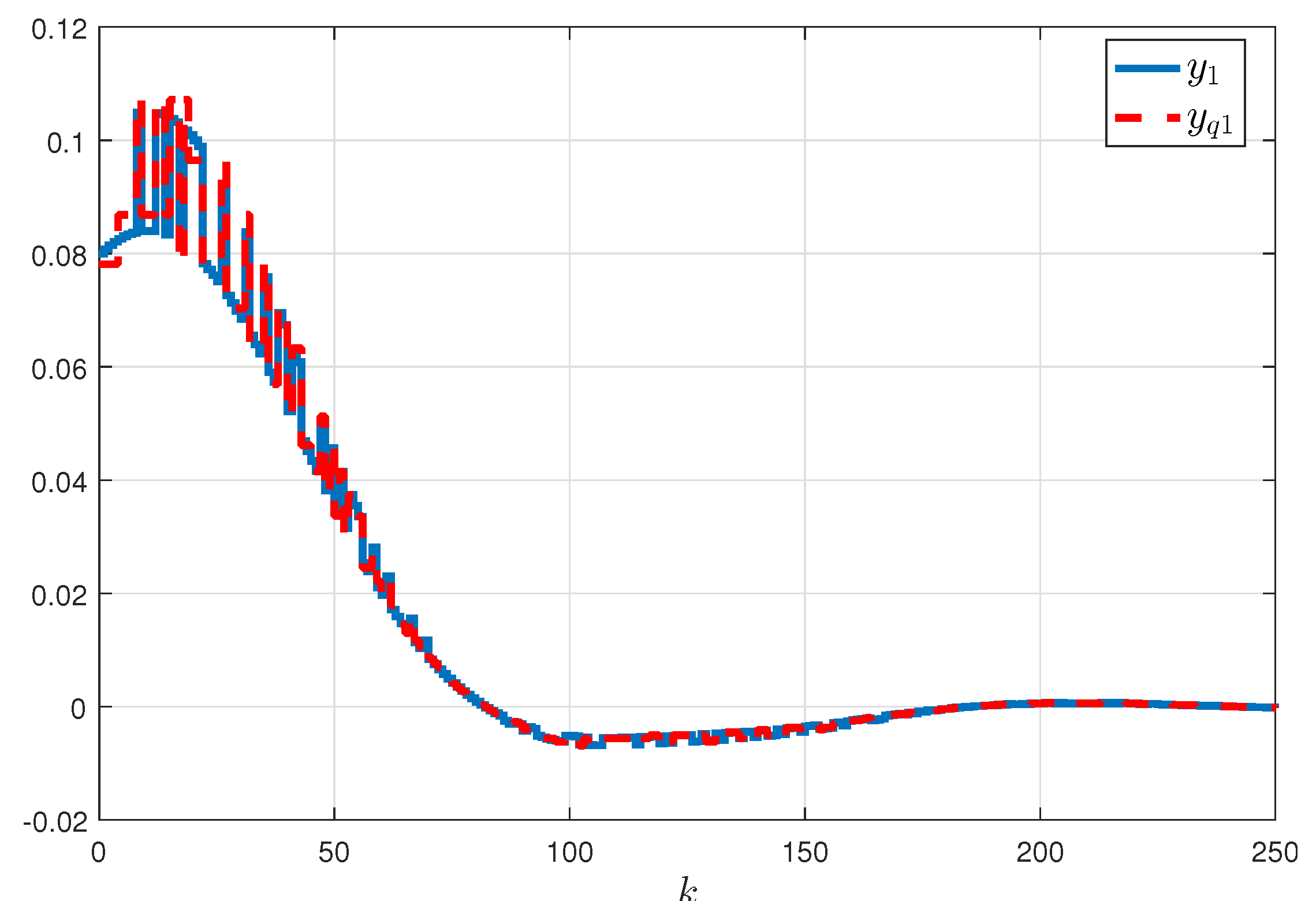
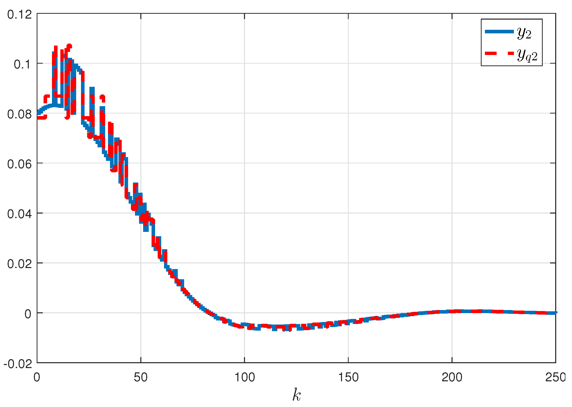
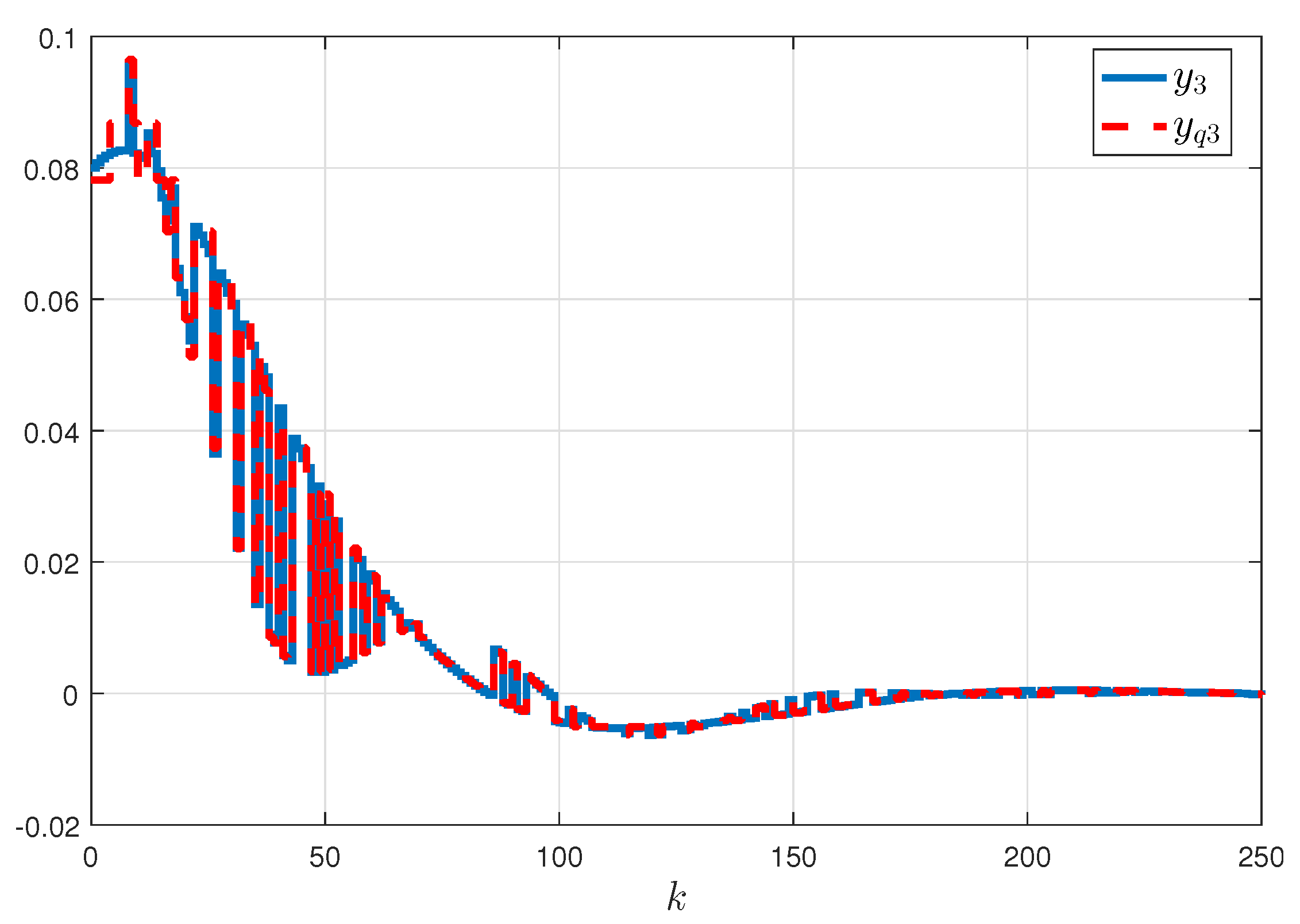
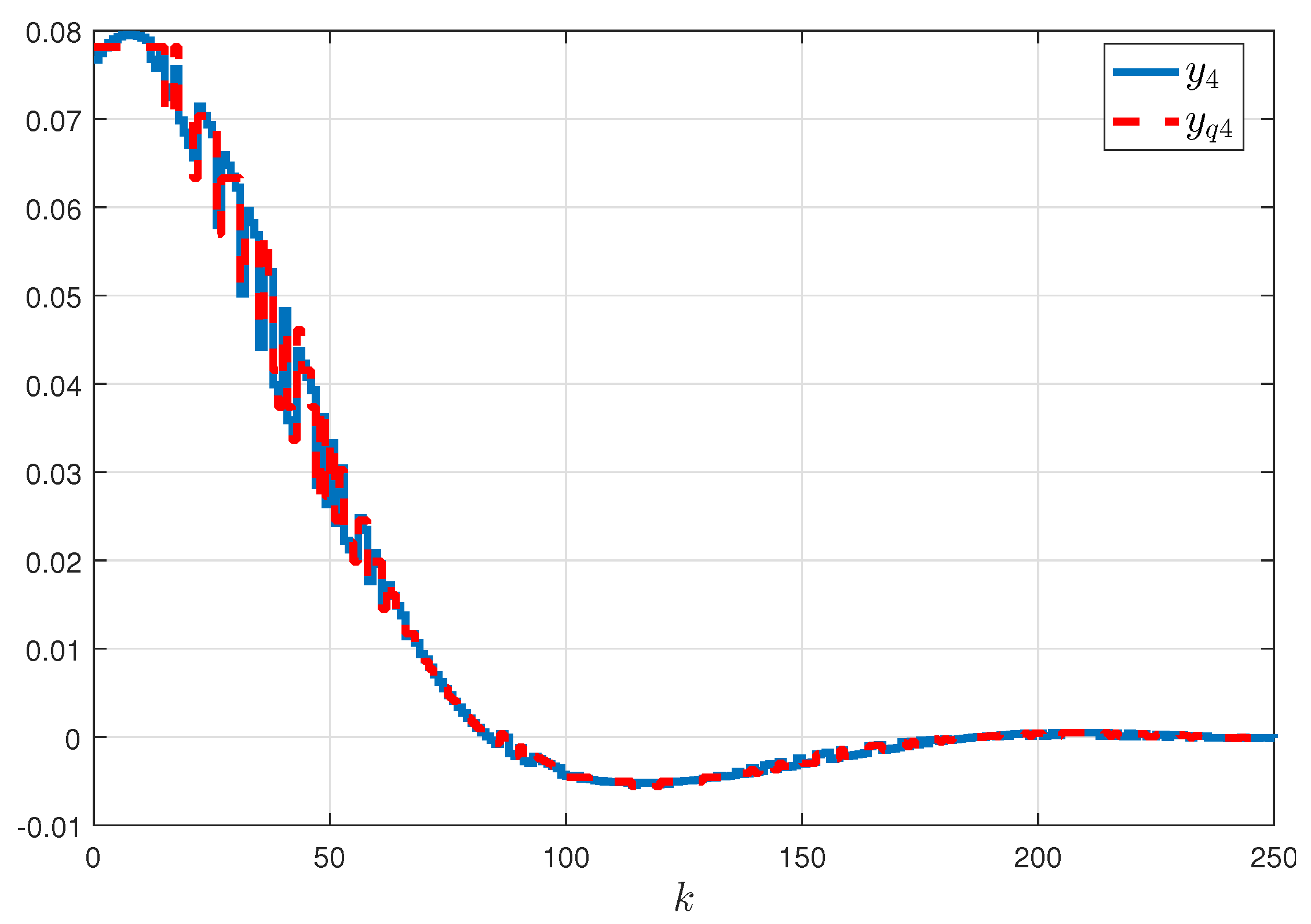
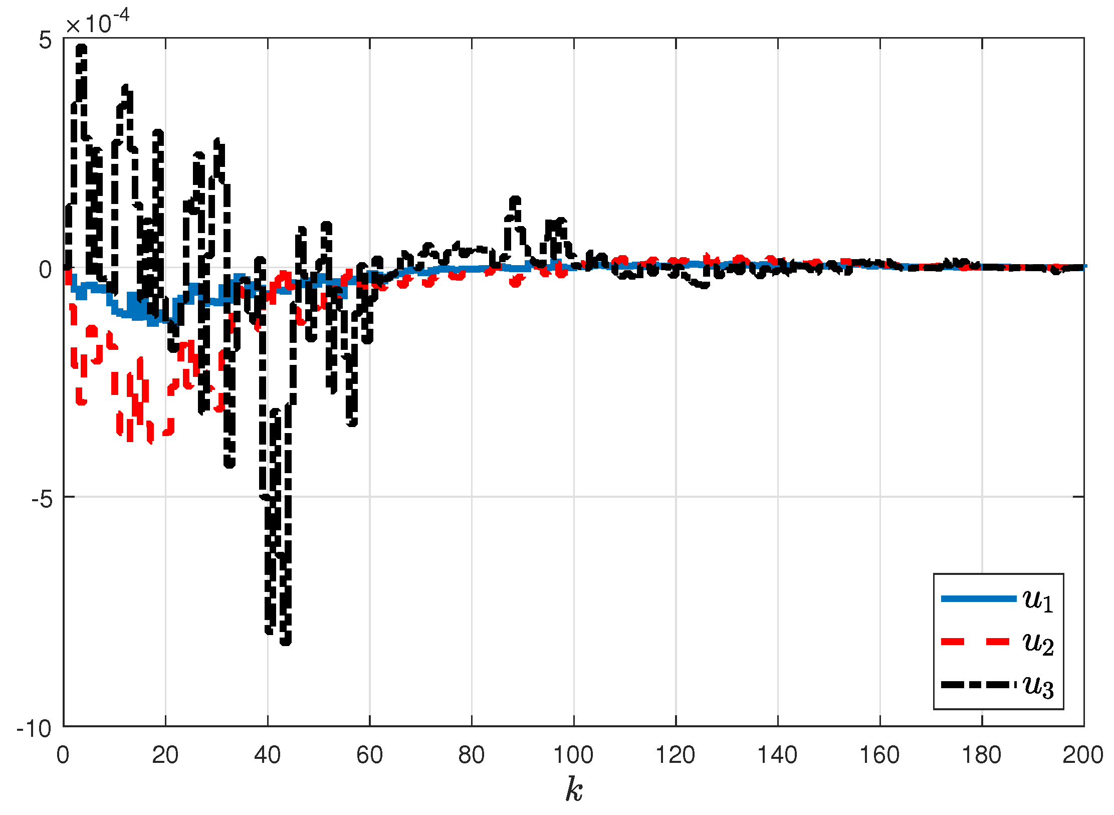
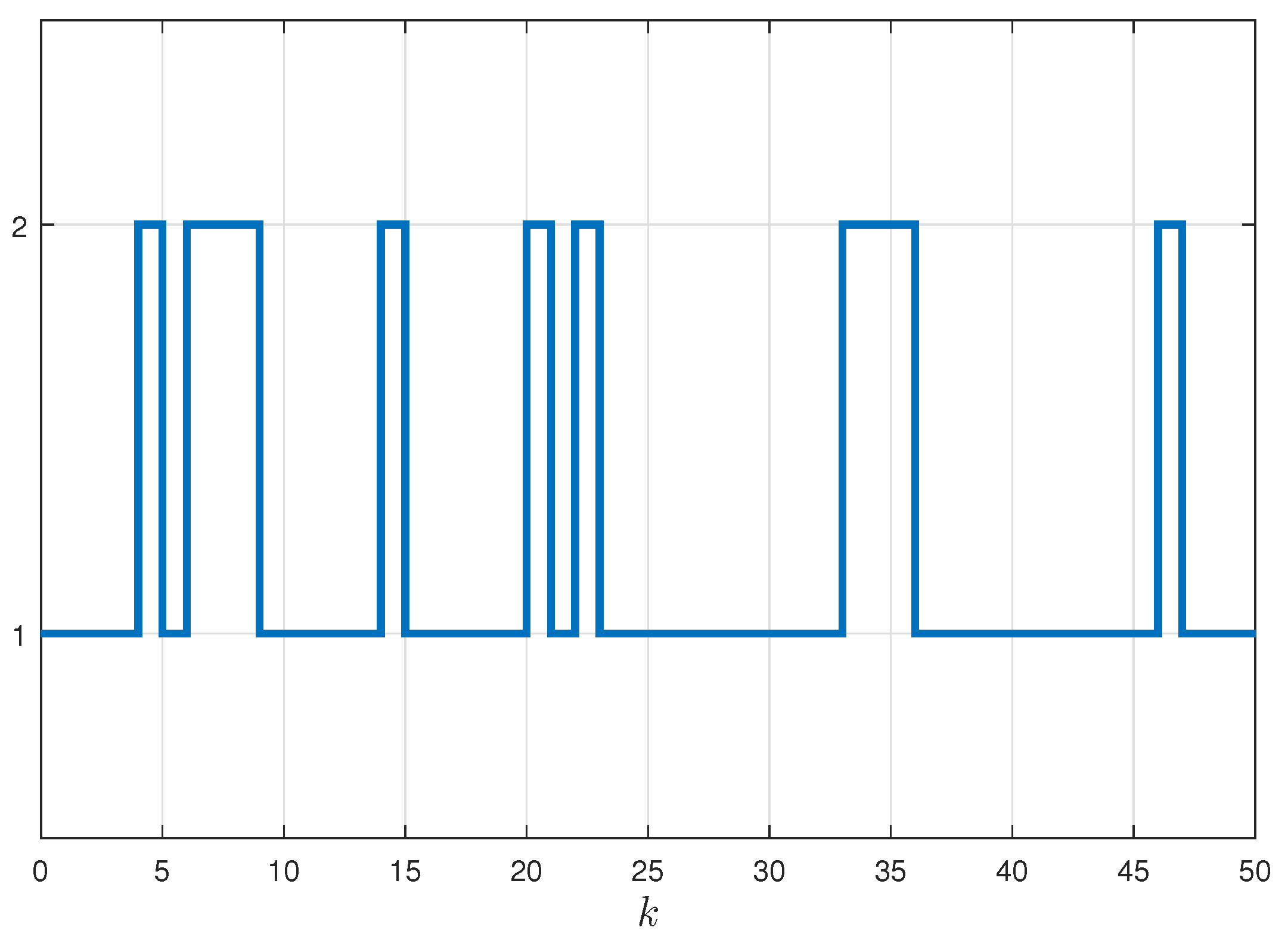
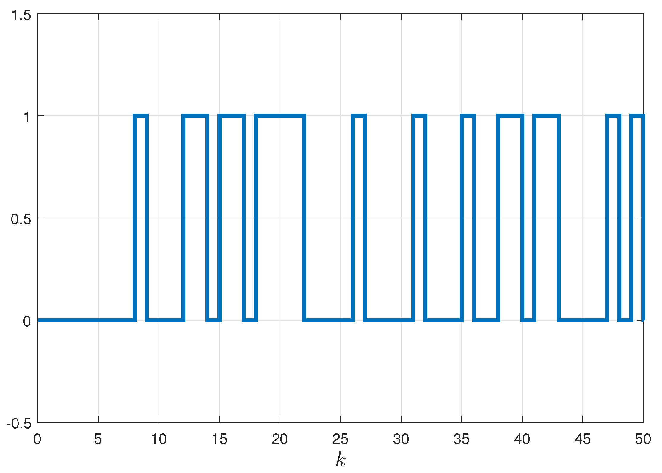
5.2. Results and Graphical Plots

As a way of demonstrating that the developed control strategy is effective, let us suppose that $w\left(k\right)=0.01sin\left(5k\right)$, and the initial condition

$x\left(0\right)=\left[\begin{array}{ccccccc}0.1& 0.1& 0.1& 0.1& 0.1& 0.1& 0.1\end{array}\right]$.

Figure 2, Figure 3, Figure 4, Figure 5, Figure 6 and Figure 7 illustrate the simulation results of the resulting closed-loop system, achieved by applying the designed fault-tolerant controller (11) to the uncertain system (Figure 1). Figure 2, Figure 3, Figure 4 and Figure 5 record the actual and quantized output responses of the system, while Figure 6, Figure 7, Figure 8 and Figure 9 show, respectively, the control input $u\left(k\right)$, the Markov chain mode of the actuator failure, and the Bernoulli distributions. The fault-tolerant dynamic output feedback controller could keep the closed-loop system dynamically stable under actuator faults, external disturbances, model uncertainties, and unmeasured states.

5.3. Comparative Explanations

With the fault-tolerant control of discrete-time descriptor systems characterized by intermittent actuator failures and unpredictable sensor non-linearities, this paper has proven effective in overcoming this challenge. In spite of various control issues for discrete-time Markovian jump systems having been explored in the literature [35,41,44], our approach differed in the following ways:

• Ref. [35] describes a discrete-time Markovian jump system with a quantized and resilient state feedback control law. As we considered a more general class of singular systems with partially measured states, our approach was more general. Additionally, random sensor non-linearity and missing data were taken into account.
• Although the reliable control problem for discrete-time descriptor systems, using a dynamic output feedback controller, had been explored in our previous work [41], the present investigation differed with the following points:
  • The intermittent actuator failures were described by a non-homogeneous Markov process with time-varying transition probabilities. Moreover, the randomly occurring sensor non-linearity, suggested in this study, was more general and might include the saturation non-linearity.
  • To handle a networked control system, the output quantization and missing data might be an effective scheme to reduce the storage space and transmission bandwidth [44].
• Between resilient controllers proposed in [35,44] and the reliable controller developed in this study, resilient controllers were employed to precisely handle gain fluctuations, whereas the reliable controller was used to compensate for failures of components in the system, especially actuators and sensors.

6. Conclusions and Future Work

6.1. Concluding Remarks

The fault-tolerant control problem presented in this paper is for discrete-time singular systems with intermittent actuator faults, randomly occurring sensor nonlinearity, and probabilistic missing data. Among the main results, the main findings are as follows: (i) Random sensor non-linearity and random missing data have been studied for singular linear systems, where related impacts have been assessed. (ii) We have discussed the intermittent actuator faults described by a non-homogenous Markov model. (iii) A dynamic output feedback controller with quantized output signals was proposed. The synthesized controller might guarantee the stochastic stability of closed-loop systems with satisfactory dissipative performance. A numerical simulation of the machine infinite bus confirmed the efficiency and potential value of the results obtained.

6.2. Limitations

This study revealed a quantized input model, which was independent of the failure modes. In spite of this, as presented in [29], this model could not be used to describe physical applications due to the absence of some available information of target modes. Accordingly, since information relating to a mode could not be transmitted correctly, the problem of combining mode-independent and mode-dependent systems when dealing with control/filtering problems pertaining to Markovian jump systems is fascinating [44]. This issue could be considered in the future.

6.3. Future Work

Other research areas that should be also pursued in the future include stabilization problems for nonlinear processes [45,46,47].

References

1. Dai, L. Singular Control Systems; Lecture Notes in Control and Information Sciences; Springer: New York, NY, USA, 1989; Volume 118. [Google Scholar]
2. Kchaou, M. Robust H Observer-Based Control for a Class of (TS) Fuzzy Descriptor Systems with Time-Varying Delay. Int. J. Fuzzy Syst. 2017, 19, 909–924. [Google Scholar] [CrossRef]
3. Zhang, Y.; Shi, P.; Agarwal, R.K.; Shi, Y. Event-Based Dissipative Analysis for Discrete Time-Delay Singular Jump Neural Networks. IEEE Trans. Neural Netw. Learn. Syst. 2020, 31, 1232–1241. [Google Scholar] [CrossRef]
4. Zhang, D.; Zhou, Z.; Jia, X. Networked fuzzy output feedback control for discrete-time Takagi-Sugeno fuzzy systems with sensor saturation and measurement noise. Inf. Sci. 2018, 457–458, 182–194. [Google Scholar] [CrossRef]
5. Wang, G.; Zhang, Q.; Yang, C. Stabilization of discrete-time singular Markovian jump repeated vector nonlinear systems. Int. J. Robust Nonlinear Control 2016, 26, 1777–1793. [Google Scholar] [CrossRef]
6. Zhang, Y.; Shi, P.; Agarwal, R.K.; Shi, Y. Event-based mixed H and passive filtering for discrete singular stochastic systems. Int. J. Control 2020, 93, 2407–2415. [Google Scholar] [CrossRef]
7. Zhang, Y.; Shi, P.; Basin, M.V. Event-based finite-time H filtering of discrete-time singular jump network systems. Int. J. Robust Nonlinear Control 2022, 32, 4038–4054. [Google Scholar] [CrossRef]
8. Kaviarasan, B.; Sakthivel, R.; Kwon, O.M. Robust fault-tolerant control for power systems against mixed actuator failures. Nonlinear Anal. Hybrid Syst. 2016, 22, 249–261. [Google Scholar] [CrossRef]
9. Kamal, E.; Aitouche, A.; Oueidat, M. Fuzzy Fault-Tolerant Control of Wind-Diesel Hybrid Systems Subject to Sensor Faults. IEEE Trans. Sustain. Energy 2013, 4, 857–866. [Google Scholar] [CrossRef]
10. Wang, S.; Jiang, Y.; Li, Y.; Liu, D. Reliable observer-based H control for discrete-time fuzzy systems with time-varying delays and stochastic actuator faults via scaled small gain theorem. Neurocomputing 2015, 147, 251–259. [Google Scholar] [CrossRef]
11. Liu, Y.; Ma, Y.; Wang, Y. Reliable sliding mode finite-time control for discrete-time singular Markovian jump systems with sensor fault and randomly occurring nonlinearities. Int. J. Robust Nonlinear Control 2018, 28, 381–402. [Google Scholar] [CrossRef]
12. Wang, Y.; Shi, P.; Yan, H. Reliable control of fuzzy singularly perturbed systems and its application to electronic circuits. IEEE Trans. Circuits Syst. I 2018, 65, 3519–3528. [Google Scholar] [CrossRef]
13. Zhao, D.; Karimi, H.R.; Sakthivel, R.; Li, Y. Non-fragile fault-tolerant control for nonlinear Markovian jump systems with intermittent actuator fault. Nonlinear Anal. Hybrid Syst. 2019, 32, 337–350. [Google Scholar] [CrossRef]
14. Cao, L.; Tao, Y.; Wang, Y.; Li, J.; Huang, B. Reliable H control for nonlinear discrete-time systems with multiple intermittent faults in sensors or actuators. Int. J. Syst. Sci. 2017, 48, 302–315. [Google Scholar] [CrossRef]
15. Tao, Y.; Shen, D.; Wang, Y.; Ye, Y. Reliable H control for uncertain nonlinear discrete-time systems subject to multiple intermittent faultsin sensors and/or actuators. J. Frankl. Inst. 2015, 352, 4721–4740. [Google Scholar] [CrossRef]
16. Li, F.; Xu, S.; Zhang, B. Resilient Asynchronous H Control for Discrete-Time Markov Jump Singularly Perturbed Systems Based on Hidden Markov Model. IEEE Trans. Syst. Man Cybern. Syst. 2020, 50, 2860–2869. [Google Scholar] [CrossRef]
17. Du, C.; Yang, C.; Li, F.; Gui, W. A Novel Asynchronous Control for Artificial Delayed Markovian Jump Systems via Output Feedback Sliding Mode Approach. IEEE Trans. Syst. Man Cybern. Syst. 2019, 49, 364–374. [Google Scholar] [CrossRef]
18. Shen, H.; Hu, X.; Wang, J.; Cao, J.; Qian, W. Non-Fragile H Synchronization for Markov Jump Singularly Perturbed Coupled Neural Networks Subject to Double-Layer Switching Regulation. IEEE Trans. Neural Netw. Learn. Syst. 2021, 1–11. [Google Scholar] [CrossRef]
19. Cheng, J.; Huang, W.; Lam, H.K.; Cao, J.; Zhang, Y. Fuzzy-Model-Based Control for Singularly Perturbed Systems with Nonhomogeneous Markov Switching: A Dropout Compensation Strategy. IEEE Trans. Fuzzy Syst. 2020, 30, 530–541. [Google Scholar] [CrossRef]
20. Wang, Z.; Rodrigues, M.; Theilliol, D.; Shen, Y. Observer-based control for singular nonhomogeneous Markov jump systems with packet losses. J. Frankl. Inst. 2018, 355, 6617–6637. [Google Scholar] [CrossRef]
21. Sathishkumar, M.; Sakthivel, R.; Kwon, O.M.; Kaviarasan, B. Finite-time mixed H and passive filtering for Takagi–Sugeno fuzzy nonhomogeneous Markovian jump systems. Int. J. Syst. Sci. 2017, 48, 1416–1427. [Google Scholar] [CrossRef]
22. Kwon, N.K.; Park, I.S.; Park, P.; Park, C. Dynamic Output-Feedback Control for Singular Markovian Jump System: LMI Approach. IEEE Trans. Autom. Control 2017, 62, 5396–5400. [Google Scholar] [CrossRef]
23. Long, S.; Zhong, S. H control for a class of discrete-time singular systems via dynamic feedback controller. Appl. Math. Lett. 2016, 58, 110–118. [Google Scholar] [CrossRef]
24. Zhang, Y.; Shi, P.; Nguang, S.K. Observer-based finite-time H control for discrete singular stochastic systems. Appl. Math. Lett. 2014, 38, 115–121. [Google Scholar] [CrossRef]
25. Chu, X.; Li, M. H non-fragile observer-based dynamic event-triggered sliding mode control for nonlinear networked systems with sensor saturation and dead-zone input. ISA Trans. 2019, 94, 93–107. [Google Scholar] [CrossRef]
26. Zuo, Z.; Wang, J.; Huang, L. Output feedback H controller design for linear discrete-time systems with sensor nonlinearities. IEE Proc.-Control Theory Appl 2005, 152, 19–26. [Google Scholar] [CrossRef]
27. Cheng, J.; Park, J.H.; Cao, J.; Qi, W. A hidden mode observation approach to finite-time SOFC of Markovian switching systems with quantization. Nonlinear Dyn. 2020, 100, 509–521. [Google Scholar] [CrossRef]
28. Shen, Y.; Wu, Z.G.; Shi, P.; Shu, Z.; Karimi, H.R. H control of Markov jump time-delay systems under asynchronous controller and quantizer. Automatica 2019, 99, 352–360. [Google Scholar] [CrossRef] [Green Version]
29. Cheng, J.; Park, J.H.; Zhao, X.; Karimi, H.R.; Cao, J. Quantized Nonstationary Filtering of Networked Markov Switching RSNSs: A Multiple Hierarchical Structure Strategy. IEEE Trans. Autom. Control 2020, 65, 4816–4823. [Google Scholar] [CrossRef]
30. Wang, Z.; Shen, B.; Shu, H.; Wei, G. Quantized H Control for Nonlinear Stochastic Time-Delay Systems With Missing Measurements. IEEE Trans. Autom. Control 2012, 57, 1431–1444. [Google Scholar] [CrossRef] [Green Version]
31. Zhang, Y.; Mu, X. Event-triggered output quantized control of discrete Markovian singular systems. Automatica 2022, 135, 109992. [Google Scholar] [CrossRef]
32. Khalil, H.K. Nonlinear Systems; Prentice-Hall: Hoboken, NJ, USA, 2002. [Google Scholar]
33. Hu, J.; Wang, Z.; Gao, H.; Stergioulas, L.K. Probability-guaranteed H finite-horizon filtering for a class of nonlinear time-varying systems with sensor saturations. Syst. Control Lett. 2012, 64, 477–484. [Google Scholar] [CrossRef] [Green Version]
34. Rathinasamy, S.; Murugesan, S.; Alzahrani, F.; Ren, Y. Quantized Finite-Time Non-fragile Filtering for Singular Markovian Jump Systems with Intermittent Measurements. Circuits Syst. Signal Process. 2019, 38, 3971–3995. [Google Scholar] [CrossRef]
35. Sathishkumar, M.; Sakthivel, R.; Alzahrani, F.S.; Kaviarasan, B.; Ren, Y. Mixed H and passivity-based resilient controller for nonhomogeneous Markov jump systems. Nonlinear Anal. Hybrid Syst. 2019, 31, 86–99. [Google Scholar] [CrossRef]
36. El-Sheikhi, F.A.; Soliman, H.M.; Ahshan, R.; Hossain, E. Regional Pole Placers of Power Systems under Random Failures/Repair Markov Jumps. Energies 2021, 14, 1989. [Google Scholar] [CrossRef]
37. Xu, S.; Lam, J. Robust Control and Filtering of Singular Systems; Springer: Berlin/Heidelberg, Germany, 2006. [Google Scholar]
38. Wu, Z.; Park, J.; Su, H.; Chu, J. Admissibility and dissipativity analysis for discrete-time singular systems with mixed time-varying delays. Appl. Math. Comput. 2012, 218, 7128–7138. [Google Scholar] [CrossRef]
39. Peterson, I. A stabilization algorithm for a class uncertain linear systems. Syst. Control Lett. 1987, 8, 351–357. [Google Scholar] [CrossRef]
40. Wang, W.; Ma, S.; Zhang, C. Stability and Static Output Feedback Stabilization for a Class of Nonlinear Discrete-Time Singular Switched Systems. Int. J. Control. Autom. Syst. 2013, 11, 1138–1148. [Google Scholar] [CrossRef]
41. Kchaou, M.; Jerbi, H.; Ali, N.B.; Alsaif, H. H Reliable Dynamic Output-Feedback Controller Design for Discrete-Time Singular Systems with Sensor Saturation. Actuators 2021, 10, 196. [Google Scholar] [CrossRef]
42. Koenig, D. Unknown input proportional multiple-integral observer design for linear descriptor systems: Application to state and fault estimation. IEEE Trans. Autom. Control 2005, 50, 212–217. [Google Scholar] [CrossRef] [Green Version]
43. Guo, S.; Jiang, B.; Zhu, F.; Wang, Z. Luenberger-like interval observer design for discrete-time descriptor linear system. Syst. Control Lett. 2019, 126, 21–27. [Google Scholar] [CrossRef]
44. Sathishkumar, M.; Sakthivel, R.; Wang, C.; Kaviarasan, B.; Marshal Anthoni, S. Non-fragile filtering for singular Markovian jump systems with missing measurements. Signal Process. 2018, 142, 125–136. [Google Scholar] [CrossRef]
45. Hamidi, F.; Aloui, M.; Jerbi, H.; Kchaou, M.; Abbassi, R.; Popescu, D.; Ben Aoun, S.; Dimon, C. Chaotic Particle Swarm Optimisation for Enlarging the Domain of Attraction of Polynomial Nonlinear Systems. Electronics 2020, 9, 10. [Google Scholar] [CrossRef]
46. Hamidi, F.; Jerbi, H.; Olteanu, S.C.; Popescu, D. An Enhanced Stabilizing Strategy for Switched Nonlinear Systems. Stud. Inform. Control 2019, 28, 391–400. [Google Scholar] [CrossRef]
47. Popescu, D.; Dimon, C.; Borne, P.; Olteanu, S.C.; Mone, M.A. Advanced Control for Hydrogen Pyrolysis Installations. Energies 2020, 13, 3270. [Google Scholar] [CrossRef]
Figure 1. Three machine infinite buses.
Mathematics 10 01872 g001
Figure 2. Actual output, y 1 , and quantized output, y q 1 .
Mathematics 10 01872 g002
Figure 3. Actual output, y 2 , and quantized output, y q 2 .
Mathematics 10 01872 g003
Figure 4. Actual output, y 3 , and quantized output, y q 3 .
Mathematics 10 01872 g004
Figure 5. Actual output, y 4 , and quantized output, y q 4 .
Mathematics 10 01872 g005
Figure 6. Input trajectories.
Mathematics 10 01872 g006
Figure 7. Mode values of Markov chains of an intermittent fault.
Mathematics 10 01872 g007
Figure 8. Bernoulli distribution variable β ( k ) .
Mathematics 10 01872 g008
Figure 9. ‘Bernoulli distribution variable θ ( k ) .
Mathematics 10 01872 g009