Identification and Classification of Aggregation Operators Using Bipolar Complex Fuzzy Settings and Their Application in Decision Support Systems

Abstract

The idea of bipolar complex fuzzy (BCF) sets, as a genuine modification of both bipolar fuzzy sets and complex fuzzy sets, gives a massive valuable framework for representing and evaluating ambiguous information. In intelligence decision making based on BCF sets, it is a critical dilemma to compare or rank positive and negative membership grades. In this framework, we deliberated various techniques for aggregating the collection of information into a singleton set, called BCF weighted arithmetic averaging (BCFWAA), BCF ordered weighted arithmetic averaging (BCFOWAA), BCF weighted geometric averaging (BCFWGA), and BCF ordered weighted geometric averaging (BCFOWGA) operators for BCF numbers (BCFNs). To illustrate the feasibility and original worth of the diagnosed approaches, we demonstrated various properties of the diagnosed operators, in addition to their capability that the evaluated value of a set of BCF numbers is a unique BCF number. Further, multiattribute decision making (“MADM”) refers to a technique employed to compute a brief and dominant assessment of opinions with multiattributes. The main influence of this theory is implementing the diagnosed theory in the field of the MADM tool using BCF settings. Finally, a benchmark dilemma is used for comparison with various prevailing techniques to justify the cogency and dominancy of the evaluated operators.

1. Introduction

The major theory of decision-making tools is gaining extensive consideration, of which multiattribute decision making (MADM) is one of the most meaningful and reliable used in many fields. MADM is a massive common genuine life technique that can be expressed as the gains of mental and reasoning procedures for the classification and verification of a suitable alternative based on defined attributes. In many situations, experts have ambiguity in representing a particular preference and accurate resolution values meaningfully if a problem study contains unreliable and problematic data. However, obtaining the beneficial optimal value using crisp is an extremely awkward task for experts. Hence, the principle of the fuzzy set (FS), diagnosed to evaluate MADM techniques, regards as awkward and ambiguous employing the supporting grade (SG) to demonstrate the level of an object involving FS theory [1]. Various investigations have been conducted on FS, for instance, fuzzy N-soft sets (FNSS) [2], hesitant FNSS [3], bibliometric overview under FSs [4], and fractional FSs [5]. Further, ambiguity and uncertainty are involved in every mathematical and genuine life issue, and in consideration of FS, dealing with awkward and unreliable information is very problematic. For this, the major targeted and well-known theory of bipolar FS (BFS) [6] was utilized to evaluate genuine life issues using positive and negative SG. However, the difference between these grades is that the positive SG is defined from the universal set to [0, 1], and the negative SG is defined from the universal set to [−1, 0]. Due to the negative SG, they have a lot of advantages compared with FSs. To enhance the feasibility in the data representation of the evaluation of the attributes and the accuracy of decision-making techniques, scholars have developed many techniques using BFS, for example, Dombi operators [7], Dombi prioritized operators [8], bipolar soft sets [9], bipolar fuzzy soft sets [10], cubic BFSs [11], averaging operators for cubic BFSs [12], extended BFSs [13], uniform for BFSs [14], 2-tuple linguistic BFSs [15], order weighted operators [16], analysis of distinct implications for BFSs [17], different types of measures for BFSs [18], bipolar hesitant fuzzy linguistic sets [19], and bipolar Pythagorean fuzzy sets [20].

With the availability of the above-cited information, there is an ambiguity to manage the periodicity that is in various genuine life dilemmas. The complex information can be considered to address the periodicity of the grades by its phase term, and also, complex information can be shown in two-dimension data. Keeping the supremacy and worth of the complex information, Ramot et al. [21] extended the range of FS (“[0, 1]”) into a range of complex FS (CFS) belonging to the unit disc in the complex plane. The mathematical structure of SG in CFS is of the form x + iy, where the values x and y are defined from the universal set to [0, 1]. In many papers, many authors have used the polar form of $x+iy$, which is $r{e}^{i\varnothing }$. In complex and diverse useful decision-making tools, CFS and specific complex fuzzy numbers have possible deficiencies, for example, interval-valued CFSs [22], complex fuzzy hypersoft sets [23], interdependency for CFSs [24], algebraic structure for CFSs [25], distance measures for CFSs [26], entropy measures for CFSs [27], and similarity measures for CFSs [28]. Additionally, ambiguity and uncertainty are involved in every mathematical and genuine life issue, and in consideration of CFS, dealing with awkward and unreliable information is very problematic. For this, the major targeted and well-known theory of bipolar CFS (BCFS) [29] was utilized to evaluate genuine life issues using positive and negative SG in the shape of complex numbers. However, the difference between these grades is that the positive SG is defined from the universal set to $\left[0, 1\left]+i\right[0, 1\right],$ and the negative SG is defined from the universal set to $\left[-1, 0\left]+i\right[-1, 0\right]$. Due to the negative SG, they have a lot of advantages compared with FSs, BFSs, and CFSs. To enhance the feasibility in the data representation of the evaluation of attributes and the accuracy of decision-making techniques, scholars have developed many techniques using BCFS, for example, Dombi aggregation operators [30] and Hamacher aggregation operators [31]. The information explained in this section is contained in three major problems.

• How do we manage the finite family of BCF numbers?
• How do we aggregate the distinct criteria values and arrange all opinion values?
• How do we give rank to alternatives for finding the beneficial decision?

Hence, the main key features of this analysis are eliminating these complications and computing a perfect and well-known technique for evaluating genuine life dilemmas very accurately.

The prevailing drawbacks, such as FSs, BFSs, and CFSs, have been extensively capable in various disciplines, while they have been limited in conditions and structures. In such structures, the data arranged based on the term are managed with only one-dimension data at a time, which are obvious loss of various kinds of information at specific periods. In genuine life, we deal with complex circumstances where it becomes necessary to add another term to the positive and negative SG. By introducing this other term/dimension, the complete data can be organized in a single term, and hence, data loss can be rejected. To demonstrate the meaning of the phase term, assume an automotive enterprise in Pakistan, where they resolve to choose the ERP software for enhancing their enterprise’s activities. Enterprises consult an expert team concerning (i) total rating and (ii) the latest version of the ERP software. This is a two-dimensional dilemma, and this is incapable of being performed correctly based on BCFSs. The theory of BCF information is a meaningful and valuable framework used for the identification and classification of the problematic and awkward information that happens in genuine life dilemmas.

The theory of the BCF set is a modified theory of BFS because the amplitude term workings the theory of BCF information, and due to this, the theory of the BCF set is massively valuable and dominant. The main difference between BCF sets and BFS is that the BCF set contains an amplitude term and the BFS does not. The amplitude and phase terms represent the real and imaginary parts in the BCF information. The phase term is not included in the theory of the BFS, and due to this issue, experts have lost a lot of information in evaluating the process of decision making. Similarly, the same cases have occurred in many places, and due to these issues, many experts have found alternatives. Further, the main importance of the phase term is explained with help of some suitable examples. For instance, someone wants to buy a car based on two important features, called model and production data, which represent the real and imaginary parts, and notices that the existing theory of the BFS has been refused. For managing such sort of issues, the theory of BCF information is massively suitable because the positive and negative membership grades in BCF information are in the shape of a complex number. Hence, the theory of BCF information is a modified version of the prevailing or traditional BFS.

Thus, motivated by the above genuine and practical examples of BCF information and decision-making procedure, this analysis deals with how to aggregate and how to find the best decision by employing the ambiguity and fuzzy data. To evaluate these complications, this analysis is focused on evaluating the above differences and proposing an alternative solution. The main purpose of this theory is described below:

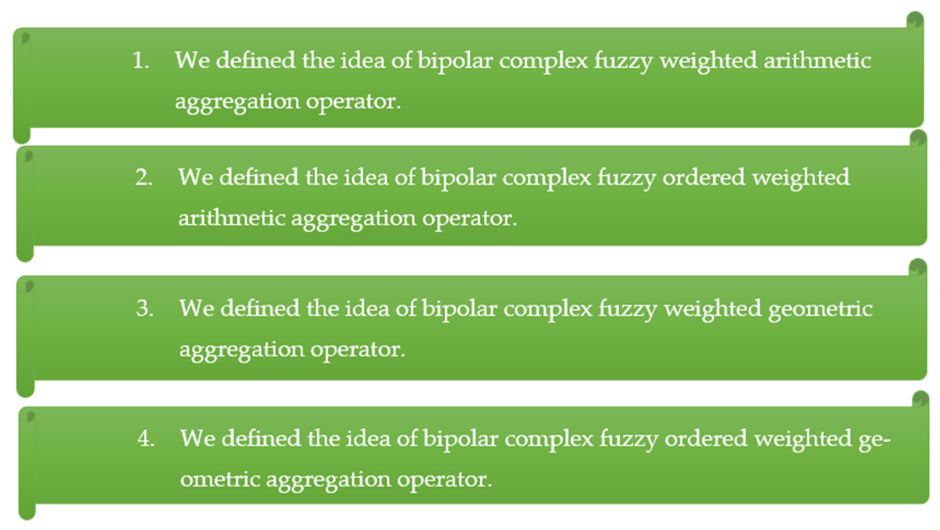
• To deliberate various techniques for aggregating the collection of information into a singleton set, called BCFWAA, BCFOWAA, BCFWGA, and BCFOWGA operators for BCFNs.
• To illustrate the feasibility and original worth of the diagnosed approaches, we demonstrated the properties (“idempotency, monotonicity, and boundedness”) and the results of the investigated work.
• MADM refers to a technique employed to compute a brief and dominant assessment of opinions with multiattributes. The main influence of this theory is implementing the diagnosed theory in the field of the MADM tool using BCF settings.
• Finally, the invented techniques are resolved by conferring with logical ranking evaluation and comparative techniques, which discovered that the ranking is the theme to a logical ranking that is encouraged by superior parallel results over a distinct framework with differences in the weights of the criteria.

The construction of this theory is developed in this fashion: In Section 2, we recall the fundamental theory of BCF setting and its operational laws. In Section 3, we deliberate various techniques for aggregating the collection of information into a singleton set, called BCFWAA, BCFOWAA, BCFWGA, and BCFOWGA operators for BCFNs. To illustrate the feasibility and original worth of the diagnosed approaches, we demonstrate the properties (“idempotency, monotonicity, and boundedness”) and the results of the investigated work. In Section 4, MADM refers to a technique employed to compute a brief and dominant assessment of opinions with multiattributes. The main influence of this theory is implementing the diagnosed theory in the field of the MADM tool using BCF settings. Finally, the invented techniques are resolved by conferring with logical ranking evaluation and comparative techniques, which discovered that the ranking is the theme to a logical ranking that is encouraged by superior parallel results over a distinct framework with differences in the weights of the criteria. In Section 5, we describe the conclusion of this article.

2. Preliminaries

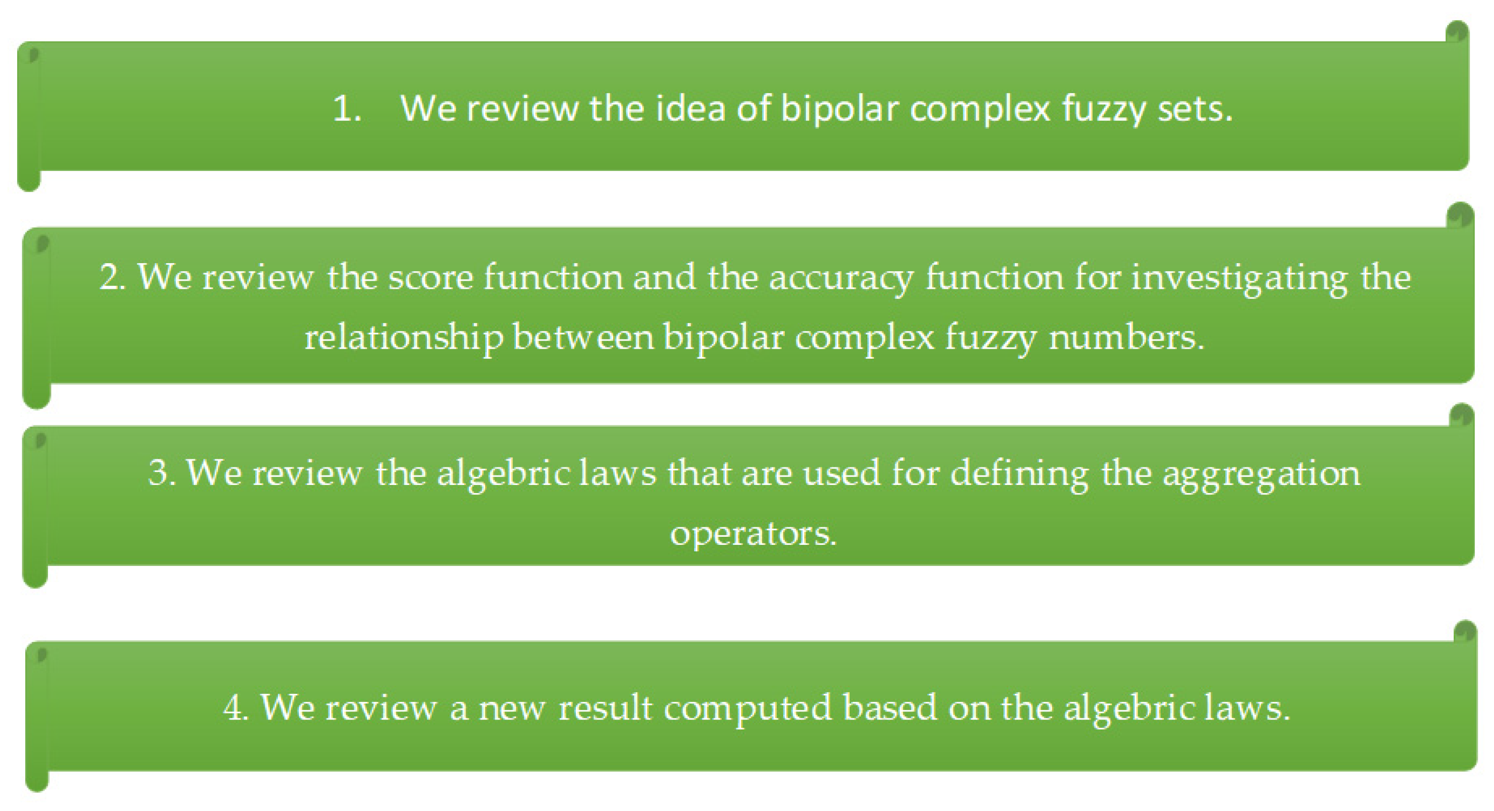
In this theory, we recall the fundamental theory of BCF setting and its operational laws. The theory of BCF information is a meaningful and valuable framework used for the identification and classification of the problematic and awkward information that happens in genuine life dilemmas.

Definition 1 ([29]).

The theory of BCF information is invented by:

$$\mathsf{Ŵ}=\left\{\left(𝜘, {\mathsf{{\rm T}}}_{P-\mathsf{Ŵ}}\left(𝜘\right), {\mathsf{{\rm T}}}_{N-\mathsf{Ŵ}}\left(𝜘\right)\right) | 𝜘\in \mathsf{Ẍ}\right\}$$

(1)

Obviously, ${\mathsf{{\rm T}}}_{P-\mathsf{Ŵ}}\left(𝜘\right)={\mathsf{{\rm T}}}_{RP-\mathsf{Ŵ}}\left(𝜘\right)+\iota {\mathsf{{\rm T}}}_{IP-\mathsf{Ŵ}}\left(𝜘\right)$and${\mathsf{{\rm T}}}_{N-\mathsf{Ŵ}}\left(𝜘\right)={\mathsf{{\rm T}}}_{RN-\mathsf{Ŵ}}\left(𝜘\right)+\iota {\mathsf{{\rm T}}}_{IN-\mathsf{Ŵ}}\left(𝜘\right)$, showing the positive and negative SG with${\mathsf{{\rm T}}}_{RP-\mathsf{Ŵ}}\left(𝜘\right),{\mathsf{{\rm T}}}_{IP-\mathsf{Ŵ}}\left(𝜘\right)\in \left[0,1\right]$, and${\mathsf{{\rm T}}}_{RN-\mathsf{Ŵ}}\left(𝜘\right),{\mathsf{{\rm T}}}_{IN-\mathsf{Ŵ}}\left(𝜘\right)\in \left[-1,0\right]$, where$\mathsf{Ŵ}=\left({\mathsf{{\rm T}}}_{P-\mathsf{Ŵ}}\left(𝜘\right),{\mathsf{{\rm T}}}_{N-\mathsf{Ŵ}}\left(𝜘\right)\right)=\left({\mathsf{{\rm T}}}_{RP-\mathsf{Ŵ}}\left(𝜘\right)+\iota {\mathsf{{\rm T}}}_{IP-\mathsf{Ŵ}}\left(𝜘\right),{\mathsf{{\rm T}}}_{RN-\mathsf{Ŵ}}\left(𝜘\right)+\iota {\mathsf{{\rm T}}}_{IN-\mathsf{Ŵ}}\left(𝜘\right)\right)$, represent the BCFNs used in all theories. The comparison between two BCF sets is very awkward; for this, we revise the theory of score and accuracy values, as shown below.

Definition 2 ([31]).

The mathematical form of the score value invented by:

$${\mathfrak{S}}_{SF}\left(\mathsf{Ŵ}\right)=\frac{1}{4}\left(2+{\mathsf{{\rm T}}}_{RP-\mathsf{Ŵ}}\left(𝜘\right)+{\mathsf{{\rm T}}}_{IP-\mathsf{Ŵ}}\left(𝜘\right)+{\mathsf{{\rm T}}}_{RN-\mathsf{Ŵ}}\left(𝜘\right)+{\mathsf{{\rm T}}}_{IN-\mathsf{Ŵ}}\left(𝜘\right)\right), {\mathfrak{S}}_{SF}\in \left[0, 1\right]$$

(2)

and the mathematical form of the accuracy value invented by:

$${\mathscr{H}}_{AF}\left(\mathsf{Ŵ}\right)=\frac{{\mathsf{{\rm T}}}_{RP-\mathsf{Ŵ}}\left(𝜘\right)+{\mathsf{{\rm T}}}_{IP-\mathsf{Ŵ}}\left(𝜘\right)+{\mathsf{{\rm T}}}_{RN-\mathsf{Ŵ}}\left(𝜘\right)+{\mathsf{{\rm T}}}_{IN-\mathsf{Ŵ}}\left(𝜘\right)}{4}, {\mathscr{H}}_{AF}\in \left[0, 1\right]$$

(3)

Using Equations (2) and (3), we demonstrate some theories, such that if ${\mathfrak{S}}_{SF}\left({\mathsf{Ŵ}}_1\right)<{\mathfrak{S}}_{SF}\left({\mathsf{Ŵ}}_2\right)$, then ${\mathsf{Ŵ}}_1<{\mathsf{Ŵ}}_2$; if ${\mathfrak{S}}_{SF}\left({\mathsf{Ŵ}}_1\right)>{\mathfrak{S}}_{SF}\left({\mathsf{Ŵ}}_2\right)$, then ${\mathsf{Ŵ}}_1>{\mathsf{Ŵ}}_2$; if ${\mathfrak{S}}_{SF}\left({\mathsf{Ŵ}}_1\right)={\mathfrak{S}}_{SF}\left({\mathsf{Ŵ}}_1\right)$, then if ${\mathscr{H}}_{AF}\left({\mathsf{Ŵ}}_1\right)<{\mathscr{H}}_{AF}\left({\mathsf{Ŵ}}_2\right),$ then ${\mathsf{Ŵ}}_1<{\mathsf{Ŵ}}_2$; if ${\mathscr{H}}_{AF}\left({\mathsf{Ŵ}}_1\right)>{\mathscr{H}}_{AF}\left({\mathsf{Ŵ}}_2\right),$ then ${\mathsf{Ŵ}}_1>{\mathsf{Ŵ}}_2$; if ${\mathscr{H}}_{AF}\left({\mathsf{Ŵ}}_1\right)={\mathscr{H}}_{AF}\left({\mathsf{Ŵ}}_2\right),$ then ${\mathsf{Ŵ}}_1={\mathsf{Ŵ}}_2$. We noticed that the BCF information is very valuable, but without defining the addition, multiplication, and scaler laws, it has no worth; therefore, we illustrate or recall some laws called algebraic laws based on BCF information. For ${\mathsf{Ŵ}}_1=\left({\mathsf{{\rm T}}}_{P-{\mathsf{Ŵ}}_1},{\mathsf{{\rm T}}}_{N-{\mathsf{Ŵ}}_1}\right)=\left({\mathsf{{\rm T}}}_{RP-{\mathsf{Ŵ}}_1}+\iota {\mathsf{{\rm T}}}_{IP-{\mathsf{Ŵ}}_1},{\mathsf{{\rm T}}}_{RN-{\mathsf{Ŵ}}_1}+\iota {\mathsf{{\rm T}}}_{IN-{\mathsf{Ŵ}}_1}\right)$ and ${\mathsf{Ŵ}}_2=\left({\mathsf{{\rm T}}}_{P-{\mathsf{Ŵ}}_2},{\mathsf{{\rm T}}}_{N-{\mathsf{Ŵ}}_2}\right)=\left({\mathsf{{\rm T}}}_{RP-{\mathsf{Ŵ}}_2}+\iota {\mathsf{{\rm T}}}_{IP-{\mathsf{Ŵ}}_2},{\mathsf{{\rm T}}}_{RN-{\mathsf{Ŵ}}_2}+\iota {\mathsf{{\rm T}}}_{IN-{\mathsf{Ŵ}}_2}\right)$ with $\lambda >0$, we have

$${\mathsf{Ŵ}}_1\oplus {\mathsf{Ŵ}}_2=\left(\begin{array}{c}{\mathsf{{\rm T}}}_{RP-{\mathsf{Ŵ}}_1}+{\mathsf{{\rm T}}}_{RP-{\mathsf{Ŵ}}_2}-{\mathsf{{\rm T}}}_{RP-{\mathsf{Ŵ}}_1}{\mathsf{{\rm T}}}_{RP-{\mathsf{Ŵ}}_2}+\iota \left({\mathsf{{\rm T}}}_{IP-{\mathsf{Ŵ}}_1}+{\mathsf{{\rm T}}}_{RP-{\mathsf{Ŵ}}_2}-{\mathsf{{\rm T}}}_{IP-{\mathsf{Ŵ}}_1}{\mathsf{{\rm T}}}_{IP-{\mathsf{Ŵ}}_2}\right), \\ -\left({\mathsf{{\rm T}}}_{RN-{\mathsf{Ŵ}}_1}{\mathsf{{\rm T}}}_{RN-{\mathsf{Ŵ}}_2}\right)+\iota \left(-\left({\mathsf{{\rm T}}}_{IN-{\mathsf{Ŵ}}_1}{\mathsf{{\rm T}}}_{IN-{\mathsf{Ŵ}}_2}\right)\right)\end{array}\right)$$

(4)

$${\mathsf{Ŵ}}_1\otimes {\mathsf{Ŵ}}_2=\left(\begin{array}{c}{\mathsf{{\rm T}}}_{RP-{\mathsf{Ŵ}}_1}{\mathsf{{\rm T}}}_{RP-{\mathsf{Ŵ}}_2}+\iota {\mathsf{{\rm T}}}_{IP-{\mathsf{Ŵ}}_1}{\mathsf{{\rm T}}}_{IP-{\mathsf{Ŵ}}_2}, \\ {\mathsf{{\rm T}}}_{RN-{\mathsf{Ŵ}}_1}+{\mathsf{{\rm T}}}_{RN-{\mathsf{Ŵ}}_2}{\mathsf{{\rm T}}}_{RN-{\mathsf{Ŵ}}_1}-{\mathsf{{\rm T}}}_{RN-{\mathsf{Ŵ}}_2}+\iota \left({\mathsf{{\rm T}}}_{IN-{\mathsf{Ŵ}}_1}+{\mathsf{{\rm T}}}_{IN-{\mathsf{Ŵ}}_2}{\mathsf{{\rm T}}}_{IN-{\mathsf{Ŵ}}_1}-{\mathsf{{\rm T}}}_{IN-{\mathsf{Ŵ}}_2}\right)\end{array}\right)$$

(5)

$$\lambda {\mathsf{Ŵ}}_1=\left(1-{\left(1-{\mathsf{{\rm T}}}_{RP-{\mathsf{Ŵ}}_1}\right)}^{\lambda }+\iota \left(1-{\left(1-{\mathsf{{\rm T}}}_{IP-{\mathsf{Ŵ}}_1}\right)}^{\lambda }\right),-{\left|{\mathsf{{\rm T}}}_{RN-{\mathsf{Ŵ}}_1}\right|}^{\lambda }+\iota \left(-{\left|{\mathsf{{\rm T}}}_{IN-{\mathsf{Ŵ}}_1}\right|}^{\lambda }\right) \right)$$

(6)

$${\mathsf{Ŵ}}_1{}^{\lambda }=\left(\left({\left({\mathsf{{\rm T}}}_{RP-{\mathsf{Ŵ}}_1}\right)}^{\lambda }+\iota {\left({\mathsf{{\rm T}}}_{IP-{\mathsf{Ŵ}}_1}\right)}^{\lambda },-1+{\left(1+{\mathsf{{\rm T}}}_{RN-{\mathsf{Ŵ}}_1}\right)}^{\lambda }+\iota \left(-1+{\left(1+{\mathsf{{\rm T}}}_{IN-{\mathsf{Ŵ}}_1}\right)}^{\lambda }\right)\right)\right)$$

(7)

The main influence of this section is available in Figure 1.

Theorem 1 ([31]).

For ${\mathsf{Ŵ}}_1=\left({\mathsf{{\rm T}}}_{P-{\mathsf{Ŵ}}_1}, {\mathsf{{\rm T}}}_{N-{\mathsf{Ŵ}}_1}\right)=\left({\mathsf{{\rm T}}}_{RP-{\mathsf{Ŵ}}_1}+\iota {\mathsf{{\rm T}}}_{IP-{\mathsf{Ŵ}}_1}, {\mathsf{{\rm T}}}_{RN-{\mathsf{Ŵ}}_1}+\iota {\mathsf{{\rm T}}}_{IN-{\mathsf{Ŵ}}_1}\right)$ and ${\mathsf{Ŵ}}_2=\left({\mathsf{{\rm T}}}_{P-{\mathsf{Ŵ}}_2}, {\mathsf{{\rm T}}}_{N-{\mathsf{Ŵ}}_2}\right)=\left({\mathsf{{\rm T}}}_{RP-{\mathsf{Ŵ}}_2}+\iota {\mathsf{{\rm T}}}_{IP-{\mathsf{Ŵ}}_2}, {\mathsf{{\rm T}}}_{RN-{\mathsf{Ŵ}}_2}+\iota {\mathsf{{\rm T}}}_{IN-{\mathsf{Ŵ}}_2}\right)$, with $\lambda , {\lambda }_1, {\lambda }_2>0$, we have

• ${\mathsf{Ŵ}}_1\oplus {\mathsf{Ŵ}}_2={\mathsf{Ŵ}}_2\oplus {\mathsf{Ŵ}}_1$;
• ${\mathsf{Ŵ}}_1\otimes {\mathsf{Ŵ}}_2=\mathsf{Ŵ}\otimes {\mathsf{Ŵ}}_1$;
• $\lambda \left({\mathsf{Ŵ}}_1\oplus {\mathsf{Ŵ}}_2\right)=\lambda {\mathsf{Ŵ}}_1\oplus \lambda {\mathsf{Ŵ}}_2$;
• ${\left({\mathsf{Ŵ}}_1\otimes {\mathsf{Ŵ}}_2\right)}^{\lambda }={\mathsf{Ŵ}}_1{}^{\lambda }\otimes {\mathsf{Ŵ}}_2{}^{\lambda }$;
• ${\lambda }_1{\mathsf{Ŵ}}_1\oplus {\lambda }_2{\mathsf{Ŵ}}_1=\left({\lambda }_1+{\lambda }_2\right){\mathsf{Ŵ}}_1$;
• ${\mathsf{Ŵ}}_1{}^{{\lambda }_1}\otimes {\mathsf{Ŵ}}_1{}^{{\lambda }_2}={\mathsf{Ŵ}}_1{}^{{\lambda }_1+{\lambda }_2}$;
• ${\left({\mathsf{Ŵ}}_2{}^{{\lambda }_1}\right)}^{{\lambda }_2}={\mathsf{Ŵ}}_2{}^{{\lambda }_1{\lambda }_2}$.

3. Aggregation Operators for BCF Settings

The idea of BCF sets, as a genuine modification of both bipolar fuzzy sets and complex fuzzy sets, gives a massive valuable framework for representing and evaluating ambiguous information. In intelligence decision making based on BCF sets, it is a critical dilemma to compare or rank positive and negative membership grades. In this framework, we deliberated various techniques for aggregating the collection of information into a singleton set, called BCFWAA, BCFOWAA, BCFWGA, and BCFOWGA operators for BCFNs. To illustrate the feasibility and original worth of the diagnosed approaches, we demonstrated various properties of the diagnosed operators, in addition to their capability that the evaluated value of a set of BCF numbers is a unique BCF number. In this article, $ð={\left({ð}_1, {ð}_1,,\dots {ð}_n \right)}^T$ is the weight vector (WV) such that ${ð}_j\in \left[0, 1\right]$ for all $j$ and ${{\displaystyle \sum }}_{j=1}^n{ð}_j=1$. The main influence of this section is available in Figure 2.

Definition 3.

For any collection of BCFNs,${\mathsf{Ŵ}}_j=\left({{\rm T}}_{P-{\mathsf{Ŵ}}_j}, {{\rm T}}_{N-{\mathsf{Ŵ}}_j}\right)=\left({{\rm T}}_{RP-{\mathsf{Ŵ}}_j}+\iota {{\rm T}}_{IP-{\mathsf{Ŵ}}_j}, {{\rm T}}_{RN-{\mathsf{Ŵ}}_j}+\iota {{\rm T}}_{IN-{\mathsf{Ŵ}}_j}\right), \left(j=1, 2, \dots , n\right)$, we have the following BCFWAA operator:

$$BCFWAA\left({\mathsf{Ŵ}}_1, {\mathsf{Ŵ}}_2, \dots , {\mathsf{Ŵ}}_n\right)=\begin{array}{c}n\\ \oplus \\ j=1\end{array}{ð}_j{\mathsf{Ŵ}}_j={ð}_1{\mathsf{Ŵ}}_1\oplus {ð}_2{\mathsf{Ŵ}}_2\oplus \dots \oplus {ð}_n{\mathsf{Ŵ}}_n$$

(8)

Theorem 2.

By employing Equation (8), we get the BCFNs and

$$BCFWAA\left({\mathsf{Ŵ}}_1, {\mathsf{Ŵ}}_2, \dots , {\mathsf{Ŵ}}_n\right)=\left(\begin{array}{c}1-{\displaystyle {\displaystyle \prod }_{j=1}^n}{\left(1-{\mathsf{{\rm T}}}_{RP-{\mathsf{Ŵ}}_j}\right)}^{{ð}_j}+\iota \left(1-{\displaystyle {\displaystyle \prod }_{j=1}^n}{\left(1-{\mathsf{{\rm T}}}_{IP-{\mathsf{Ŵ}}_j}\right)}^{{ð}_j}\right),\\ -{\displaystyle {\displaystyle \prod }_{j=1}^n}{\left|{\mathsf{{\rm T}}}_{RN-{\mathsf{Ŵ}}_j}\right|}^{{ð}_j}+\iota \left(-{\displaystyle {\displaystyle \prod }_{j=1}^n}{\left|{\mathsf{{\rm T}}}_{IN-{\mathsf{Ŵ}}_j}\right|}^{{ð}_j}\right)\end{array}\right)$$

(9)

Proof. 

By employing the well-known technique, called mathematical induction, to prove Equation (9), assume, for n = 2, we have

$${ð}_1{\mathsf{Ŵ}}_1=\left(\begin{array}{c}1-{\left(1-{\mathsf{{\rm T}}}_{RP-{\mathsf{Ŵ}}_1}\right)}^{{ð}_1}+\iota \left(1-{\left(1-{\mathsf{{\rm T}}}_{IP-{\mathsf{Ŵ}}_1}\right)}^{{ð}_1}\right),\\ -{\left|{\mathsf{{\rm T}}}_{RN-{\mathsf{Ŵ}}_1}\right|}^{{ð}_1}+\iota \left(-{\left|{\mathsf{{\rm T}}}_{IN-{\mathsf{Ŵ}}_1}\right|}^{{ð}_1}\right) \end{array}\right)$$

$${ð}_2{\mathsf{Ŵ}}_2=\left(\begin{array}{c}1-{\left(1-{\mathsf{{\rm T}}}_{RP-{\mathsf{Ŵ}}_2}\right)}^{{ð}_2}+\iota \left(1-{\left(1-{\mathsf{{\rm T}}}_{IP-{\mathsf{Ŵ}}_2}\right)}^{{ð}_2}\right),\\ -{\left|{\mathsf{{\rm T}}}_{RN-{\mathsf{Ŵ}}_2}\right|}^{{ð}_2}+\iota \left(-{\left|{\mathsf{{\rm T}}}_{IN-{\mathsf{Ŵ}}_2}\right|}^{{ð}_2}\right) \end{array}\right)$$

$$\begin{array}{c}{ð}_1{\mathsf{Ŵ}}_1\oplus {ð}_2{\mathsf{Ŵ}}_2=\left(\begin{array}{c}1-{\left(1-{\mathsf{{\rm T}}}_{RP-{\mathsf{Ŵ}}_1}\right)}^{{ð}_1}+\iota \left(1-{\left(1-{\mathsf{{\rm T}}}_{IP-{\mathsf{Ŵ}}_1}\right)}^{{ð}_1}\right),\\ -{\left|{\mathsf{{\rm T}}}_{RN-{\mathsf{Ŵ}}_1}\right|}^{{ð}_1}+\iota \left(-{\left|{\mathsf{{\rm T}}}_{IN-{\mathsf{Ŵ}}_1}\right|}^{{ð}_1}\right) \end{array}\right)\\ \hspace{1em}\hspace{1em}\hspace{1em}\hspace{1em}\hspace{1em}\oplus \left(\begin{array}{c}1-{\left(1-{\mathsf{{\rm T}}}_{RP-{\mathsf{Ŵ}}_2}\right)}^{{ð}_2}+\iota \left(1-{\left(1-{\mathsf{{\rm T}}}_{IP-{\mathsf{Ŵ}}_2}\right)}^{{ð}_2}\right),\\ -{\left|{\mathsf{{\rm T}}}_{RN-{\mathsf{Ŵ}}_2}\right|}^{{ð}_2}+\iota \left(-{\left|{\mathsf{{\rm T}}}_{IN-{\mathsf{Ŵ}}_2}\right|}^{{ð}_2}\right) \end{array}\right)\\ =\left(\begin{array}{c}1-{\left(1-{\mathsf{{\rm T}}}_{RP-{\mathsf{Ŵ}}_1}\right)}^{{ð}_1}{\left(1-{\mathsf{{\rm T}}}_{RP-{\mathsf{Ŵ}}_2}\right)}^{{ð}_2}+\iota \left(1-{\left(1-{\mathsf{{\rm T}}}_{IP-{\mathsf{Ŵ}}_1}\right)}^{{ð}_1}{\left(1-{\mathsf{{\rm T}}}_{IP-{\mathsf{Ŵ}}_2}\right)}^{{ð}_2}\right)\\ -\left(\left(-{\left|{\mathsf{{\rm T}}}_{RN-{\mathsf{Ŵ}}_j}\right|}^{{ð}_2}\right)\left(-{\left|{\mathsf{{\rm T}}}_{IN-{\mathsf{Ŵ}}_j}\right|}^{{ð}_2}\right)\right)\end{array}\right)\\ =\left(\begin{array}{c}1-{\displaystyle {\displaystyle \prod }_{j=1}^2}{\left(1-{\mathsf{{\rm T}}}_{RP-{\mathsf{Ŵ}}_j}\right)}^{{ð}_j}+\iota \left(1-{\displaystyle {\displaystyle \prod }_{j=1}^2}{\left(1-{\mathsf{{\rm T}}}_{IP-{\mathsf{Ŵ}}_j}\right)}^{{ð}_j}\right),\\ -{\displaystyle {\displaystyle \prod }_{j=1}^2}{\left|{\mathsf{{\rm T}}}_{RN-{\mathsf{Ŵ}}_j}\right|}^{{ð}_j}+\iota \left(-{\displaystyle {\displaystyle \prod }_{j=1}^2}{\left|{\mathsf{{\rm T}}}_{IN-{\mathsf{Ŵ}}_j}\right|}^{{ð}_j}\right)\end{array}\right)\end{array}$$

Now suppose Equation (9) is true for n = K, that is,

$$BCFWAA\left({\mathsf{Ŵ}}_1, {\mathsf{Ŵ}}_2, \dots , {\mathsf{Ŵ}}_{\mathsf{{\rm K}}}\right)=\left(\begin{array}{c}1-{\displaystyle {\displaystyle \prod }_{j=1}^{\mathsf{{\rm K}}}}{\left(1-{\mathsf{{\rm T}}}_{RP-{\mathsf{Ŵ}}_j}\right)}^{{ð}_j}+\iota \left(1-{\displaystyle {\displaystyle \prod }_{j=1}^{\mathsf{{\rm K}}}}{\left(1-{\mathsf{{\rm T}}}_{IP-{\mathsf{Ŵ}}_j}\right)}^{{ð}_j}\right),\\ -{\displaystyle {\displaystyle \prod }_{j=1}^{\mathsf{{\rm K}}}}{\left|{\mathsf{{\rm T}}}_{RN-{\mathsf{Ŵ}}_j}\right|}^{{ð}_j}+\iota \left(-{\displaystyle {\displaystyle \prod }_{j=1}^{\mathsf{{\rm K}}}}{\left|{\mathsf{{\rm T}}}_{IN-{\mathsf{Ŵ}}_j}\right|}^{{ð}_j}\right)\end{array}\right)$$

Now for n = K + 1, we have

$$\begin{array}{c}BCFWAA\left({\mathsf{Ŵ}}_1, {\mathsf{Ŵ}}_2, \dots ,{\mathsf{Ŵ}}_{\mathsf{{\rm K}}}, {\mathsf{Ŵ}}_{\mathsf{{\rm K}}+1}\right)\\ \hspace{1em}\hspace{1em}\hspace{1em}\hspace{1em}\hspace{1em}\hspace{1em}\hspace{1em}\hspace{1em}\hspace{1em}\hspace{1em}\hspace{1em}\hspace{1em}\hspace{1em}\hspace{1em}\hspace{1em}\hspace{1em}\hspace{1em}\hspace{1em}\hspace{1em}\hspace{1em}\hspace{1em}\hspace{1em}\hspace{1em}\hspace{1em}=\left(\begin{array}{c}1-{\displaystyle {\displaystyle \prod }_{j=1}^{\mathsf{{\rm K}}}}{\left(1-{\mathsf{{\rm T}}}_{RP-{\mathsf{Ŵ}}_j}\right)}^{{ð}_j}+\iota \left(1-{\displaystyle {\displaystyle \prod }_{j=1}^{\mathsf{{\rm K}}}}{\left(1-{\mathsf{{\rm T}}}_{IP-{\mathsf{Ŵ}}_j}\right)}^{{ð}_j}\right),\\ -{\displaystyle {\displaystyle \prod }_{j=1}^{\mathsf{{\rm K}}}}{\left|{\mathsf{{\rm T}}}_{RN-{\mathsf{Ŵ}}_j}\right|}^{{ð}_j}+\iota \left(-{\displaystyle {\displaystyle \prod }_{j=1}^{\mathsf{{\rm K}}}}{\left|{\mathsf{{\rm T}}}_{IN-{\mathsf{Ŵ}}_j}\right|}^{{ð}_j}\right)\end{array}\right)\\ \hspace{1em}\hspace{1em}\hspace{1em}\hspace{1em}\hspace{1em}\hspace{1em}\hspace{1em}\hspace{1em}\hspace{1em}\hspace{1em}\hspace{1em}\hspace{1em}\hspace{1em}\hspace{1em}\hspace{1em}\hspace{1em}\hspace{1em}\hspace{1em}\hspace{1em}\oplus \left(\begin{array}{c}+\iota \left(1-{\left(1-{\mathsf{{\rm T}}}_{IP-{\mathsf{Ŵ}}_{\mathsf{{\rm K}}+1}}\right)}^{{ð}_{\mathsf{{\rm K}}+1}}\right),\\ -\left({\left|{\mathsf{{\rm T}}}_{RN-{\mathsf{Ŵ}}_{\mathsf{{\rm K}}+1}}\right|}^{{ð}_{\mathsf{{\rm K}}+1}}\right)+\iota \left(-\left({\left|{\mathsf{{\rm T}}}_{IN-{\mathsf{Ŵ}}_{\mathsf{{\rm K}}+1}}\right|}^{{ð}_{\mathsf{{\rm K}}+1}}\right)\right)\end{array}\right)\\ =(\begin{array}{c}\left(\left(1-{\displaystyle {\displaystyle \prod }_{j=1}^{\mathsf{{\rm K}}}}{\left(1-{\mathsf{{\rm T}}}_{RP-{\mathsf{Ŵ}}_j}\right)}^{{ð}_j}\right)+1-{\left(1-{\mathsf{{\rm T}}}_{RP-{\mathsf{Ŵ}}_{\mathsf{{\rm K}}+1}}\right)}^{{ð}_{\mathsf{{\rm K}}+1}}-\left(1-{\left(1-{\mathsf{{\rm T}}}_{RP-{\mathsf{Ŵ}}_{\mathsf{{\rm K}}+1}}\right)}^{{ð}_{\mathsf{{\rm K}}+1}}\right)\left(1-{\displaystyle {\displaystyle \prod }_{j=1}^{\mathsf{{\rm K}}}}{\left(1-{\mathsf{{\rm T}}}_{RP-{\mathsf{Ŵ}}_j}\right)}^{{ð}_j}\right)\right)+\\ \iota \left(\left(1-{\displaystyle {\displaystyle \prod }_{j=1}^{\mathsf{{\rm K}}}}{\left(1-{\mathsf{{\rm T}}}_{IP-{\mathsf{Ŵ}}_j}\right)}^{{ð}_j}\right)+1-{\left(1-{\mathsf{{\rm T}}}_{IP-{\mathsf{Ŵ}}_{\mathsf{{\rm K}}+1}}\right)}^{{ð}_{\mathsf{{\rm K}}+1}}-\left(1-{\left(1-{\mathsf{{\rm T}}}_{IP-{\mathsf{Ŵ}}_{\mathsf{{\rm K}}+1}}\right)}^{{ð}_{\mathsf{{\rm K}}+1}}\right)\left(1-{\displaystyle {\displaystyle \prod }_{j=1}^{\mathsf{{\rm K}}}}{\left(1-{\mathsf{{\rm T}}}_{IP-{\mathsf{Ŵ}}_j}\right)}^{{ð}_j}\right)\right),\\ -\left({\displaystyle {\displaystyle \prod }_{j=1}^{\mathsf{{\rm K}}}}{\left|{\mathsf{{\rm T}}}_{RN-{\mathsf{Ŵ}}_j}\right|}^{{ð}_j}{\left|{\mathsf{{\rm T}}}_{RN-{\mathsf{Ŵ}}_{\mathsf{{\rm K}}+1}}\right|}^{{ð}_{\mathsf{{\rm K}}+1}}\right)+\iota \left(-\left({\displaystyle {\displaystyle \prod }_{j=1}^{\mathsf{{\rm K}}}}{\left|{\mathsf{{\rm T}}}_{IN-{\mathsf{Ŵ}}_j}\right|}^{{ð}_j}{\left|{\mathsf{{\rm T}}}_{IN-{\mathsf{Ŵ}}_{\mathsf{{\rm K}}+1}}\right|}^{{ð}_{\mathsf{{\rm K}}+1}}\right)\right)\end{array}\\ \hspace{1em}\hspace{1em}\hspace{1em}\hspace{1em}\hspace{1em}\hspace{1em}\hspace{1em}\hspace{1em}\hspace{1em}\hspace{1em}\hspace{1em}\hspace{1em}\hspace{1em}\hspace{1em}=\left(\begin{array}{c}1-{\displaystyle {\displaystyle \prod }_{j=1}^{\mathsf{{\rm K}}}}{\left(1-{\mathsf{{\rm T}}}_{RP-{\mathsf{Ŵ}}_j}\right)}^{{ð}_j}{\left(1-{\mathsf{{\rm T}}}_{RP-{\mathsf{Ŵ}}_{\mathsf{{\rm K}}+1}}\right)}^{{ð}_{\mathsf{{\rm K}}+1}}\\ +\iota \left(1-{\displaystyle {\displaystyle \prod }_{j=1}^{\mathsf{{\rm K}}}}{\left(1-{\mathsf{{\rm T}}}_{IP-{\mathsf{Ŵ}}_j}\right)}^{{ð}_j}{\left(1-{\mathsf{{\rm T}}}_{IP-{\mathsf{Ŵ}}_{\mathsf{{\rm K}}+1}}\right)}^{{ð}_{\mathsf{{\rm K}}+1}}\right),\\ -{\displaystyle {\displaystyle \prod }_{j=1}^{\mathsf{{\rm K}}}}{\left|{\mathsf{{\rm T}}}_{RN-{\mathsf{Ŵ}}_j}\right|}^{{ð}_j}{\left|{\mathsf{{\rm T}}}_{RN-{\mathsf{Ŵ}}_{\mathsf{{\rm K}}+1}}\right|}^{{ð}_{\mathsf{{\rm K}}+1}}\\ +\iota \left(-{\displaystyle {\displaystyle \prod }_{j=1}^{\mathsf{{\rm K}}}}{\left|{\mathsf{{\rm T}}}_{IN-{\mathsf{Ŵ}}_j}\right|}^{{ð}_j}{\left|{\mathsf{{\rm T}}}_{IN-{\mathsf{Ŵ}}_{\mathsf{{\rm K}}+1}}\right|}^{{ð}_{\mathsf{{\rm K}}+1}}\right)\end{array}\right)\\ \hspace{1em}\hspace{1em}\hspace{1em}\hspace{1em}\hspace{1em}\hspace{1em}\hspace{1em}\hspace{1em}\hspace{1em}\hspace{1em}\hspace{1em}\hspace{1em}\hspace{1em}\hspace{1em}=\left(\begin{array}{c}1-{\displaystyle {\displaystyle \prod }_{j=1}^{\mathsf{{\rm K}}+1}}{\left(1-{\mathsf{{\rm T}}}_{RP-{\mathsf{Ŵ}}_j}\right)}^{{ð}_j}+\iota \left(1-{\displaystyle {\displaystyle \prod }_{j=1}^{\mathsf{{\rm K}}+1}}{\left(1-{\mathsf{{\rm T}}}_{IP-{\mathsf{Ŵ}}_j}\right)}^{{ð}_j}\right),\\ -{\displaystyle {\displaystyle \prod }_{j=1}^{\mathsf{{\rm K}}+1}}{\left|{\mathsf{{\rm T}}}_{RN-{\mathsf{Ŵ}}_j}\right|}^{{ð}_j}+\iota \left(-{\displaystyle {\displaystyle \prod }_{j=1}^{\mathsf{{\rm K}}+1}}{\left|{\mathsf{{\rm T}}}_{IN-{\mathsf{Ŵ}}_j}\right|}^{{ð}_j}\right)\end{array}\right)\end{array}$$

This shows that Equation (9) holds for n ≥ 0. □

Theorem 3 (Idempotency property).

For any collection of BCFNs,${\mathsf{Ŵ}}_j=\left({{\rm T}}_{P-{\mathsf{Ŵ}}_j},{{\rm T}}_{N-{\mathsf{Ŵ}}_j}\right)=\left({{\rm T}}_{RP-{\mathsf{Ŵ}}_j}+{\iota {\rm T}}_{IP-{\mathsf{Ŵ}}_j},{{\rm T}}_{RN-{\mathsf{Ŵ}}_j}+{\iota {\rm T}}_{IN-{\mathsf{Ŵ}}_j}\right),\left(j=1,2,\dots ,n\right)$, if ${\mathsf{Ŵ}}_j=\mathsf{Ŵ}\forall j$, then

$$BCFWAA\left({\mathsf{Ŵ}}_1,{\mathsf{Ŵ}}_2,\dots ,{\mathsf{Ŵ}}_{\mathrm{n}}\right)=\mathsf{Ŵ}$$

(10)

Proof. 

Assuming that ${\mathsf{Ŵ}}_j=\mathsf{Ŵ}$, then

$$\begin{array}{c}BCFWAA\left({\mathsf{Ŵ}}_1, {\mathsf{Ŵ}}_2, \dots , {\mathsf{Ŵ}}_n\right)=\left(\begin{array}{c}1-{\displaystyle {\displaystyle \prod }_{j=1}^n}{\left(1-{\mathsf{{\rm T}}}_{RP-\mathsf{Ŵ}}\right)}^{{ð}_j}+\iota \left(1-{\displaystyle {\displaystyle \prod }_{j=1}^n}{\left(1-{\mathsf{{\rm T}}}_{IP-\mathsf{Ŵ}}\right)}^{{ð}_j}\right),\\ -{\displaystyle {\displaystyle \prod }_{j=1}^n}{\left|{\mathsf{{\rm T}}}_{RN-\mathsf{Ŵ}}\right|}^{{ð}_j}+\iota \left(-{\displaystyle {\displaystyle \prod }_{j=1}^n}{\left|{\mathsf{{\rm T}}}_{IN-\mathsf{Ŵ}}\right|}^{{ð}_j}\right)\end{array}\right)\\ =\left(\begin{array}{c}1-{\left(1-{\mathsf{{\rm T}}}_{RP-\mathsf{Ŵ}}\right)}^{{\displaystyle {\displaystyle \sum }_{j=1}^n}{ð}_j}+\iota \left(1-{\left(1-{\mathsf{{\rm T}}}_{IP-\mathsf{Ŵ}}\right)}^{{\displaystyle {\displaystyle \sum }_{j=1}^n}{ð}_j}\right),\\ -{\left|{\mathsf{{\rm T}}}_{RN-\mathsf{Ŵ}}\right|}^{{\displaystyle \sum }_{j=1}^n{ð}_j}+\iota \left(-{\left|{\mathsf{{\rm T}}}_{IN-\mathsf{Ŵ}}\right|}^{{\displaystyle \sum }_{j=1}^n{ð}_j}\right)\end{array}\right)\\ =\left(\begin{array}{c}1-\left(1-{\mathsf{{\rm T}}}_{RP-\mathsf{Ŵ}}\right)+\iota \left(1-\left(1-{\mathsf{{\rm T}}}_{IP-\mathsf{Ŵ}}\right)\right),\\ {\mathsf{{\rm T}}}_{RN-\mathsf{Ŵ}}+\iota \left({\mathsf{{\rm T}}}_{IN-\mathsf{Ŵ}}\right)\end{array}\right)\\ =\left({\mathsf{{\rm T}}}_{RP-\mathsf{Ŵ}}+\iota {\mathsf{{\rm T}}}_{IP-\mathsf{Ŵ}}, {\mathsf{{\rm T}}}_{RN-\mathsf{Ŵ}}+\iota {\mathsf{{\rm T}}}_{IN-\mathsf{Ŵ}}\right).\end{array}$$

 □

Theorem 4 (Monotonicity property).

For any two collections of BCFNs, ${\mathsf{Ŵ}}_{\mathrm{j}}=\left({\mathsf{{\rm T}}}_{\mathrm{P}-{\mathsf{Ŵ}}_{\mathrm{j}}},{\mathsf{{\rm T}}}_{\mathrm{N}-{\mathsf{Ŵ}}_{\mathrm{j}}}\right)=\left({\mathsf{{\rm T}}}_{\mathrm{RP}-{\mathsf{Ŵ}}_{\mathrm{j}}}+{\mathsf{\iota }\mathsf{{\rm T}}}_{\mathrm{IP}-{\mathsf{Ŵ}}_{\mathrm{j}}},{\mathsf{{\rm T}}}_{\mathrm{RN}-{\mathsf{Ŵ}}_{\mathrm{j}}}+{\mathsf{\iota }\mathsf{{\rm T}}}_{\mathrm{IN}-{\mathsf{Ŵ}}_{\mathrm{j}}}\right)$ and${\mathsf{Ŵ}}_{\mathrm{j}}^{\text{’}}=\left({\mathsf{{\rm T}}}_{\mathrm{P}-{\mathsf{Ŵ}}_{\mathrm{j}}^{\text{’}}},{\mathsf{{\rm T}}}_{\mathrm{N}-{\mathsf{Ŵ}}_{\mathrm{j}}^{\text{’}}}\right)=\left({\mathsf{{\rm T}}}_{\mathrm{RP}-{\mathsf{Ŵ}}_{\mathrm{j}}^{\text{’}}}+{\mathsf{\iota }\mathsf{{\rm T}}}_{\mathrm{IP}-{\mathsf{Ŵ}}_{\mathrm{j}}^{\text{’}}},{\mathsf{{\rm T}}}_{\mathrm{RN}-{\mathsf{Ŵ}}_{\mathrm{j}}^{\text{’}}}+{\mathsf{\iota }\mathsf{{\rm T}}}_{\mathrm{IN}-{\mathsf{Ŵ}}_{\mathrm{j}}^{\text{’}}}\right),\left(\mathrm{j}=1,2,\dots ,\mathrm{n}\right)$, if ${\mathsf{{\rm T}}}_{\mathrm{RP}-{\mathsf{Ŵ}}_{\mathrm{j}}}\le {\mathsf{{\rm T}}}_{\mathrm{RP}-{\mathsf{Ŵ}}_{\mathrm{j}}^{\text{’}}}$, ${\mathsf{{\rm T}}}_{\mathrm{IP}-{\mathsf{Ŵ}}_{\mathrm{j}}}\le {\mathsf{{\rm T}}}_{\mathrm{IP}-{\mathsf{Ŵ}}_{\mathrm{j}}^{\text{’}}}$, ${\mathsf{{\rm T}}}_{\mathrm{RN}-{\mathsf{Ŵ}}_{\mathrm{j}}}\le {\mathsf{{\rm T}}}_{\mathrm{RN}-{\mathsf{Ŵ}}_{\mathrm{j}}^{\text{’}}}$, ${\mathsf{{\rm T}}}_{\mathrm{IN}-{\mathsf{Ŵ}}_{\mathrm{j}}}\le {\mathsf{{\rm T}}}_{\mathrm{IN}-{\mathsf{Ŵ}}_{\mathrm{j}}^{\text{’}}}$ for all$j$, then

$$BCFWAA\left({\mathsf{Ŵ}}_1, {\mathsf{Ŵ}}_2, \dots , {\mathsf{Ŵ}}_n\right)\le BCFWAA\left({\mathsf{Ŵ}}_1^{’}, {\mathsf{Ŵ}}_2^{’}, \dots , {\mathsf{Ŵ}}_n^{’}\right)$$

(11)

Proof. 

Assuming that ${\mathsf{{\rm T}}}_{RP-{\mathsf{Ŵ}}_j}\le {\mathsf{{\rm T}}}_{RP-{\mathsf{Ŵ}}_j^{\text{’}}}$, ${\mathsf{{\rm T}}}_{IP-{\mathsf{Ŵ}}_j}\le {\mathsf{{\rm T}}}_{IP-{\mathsf{Ŵ}}_j^{\text{’}}}$, ${\mathsf{{\rm T}}}_{RN-{\mathsf{Ŵ}}_j}\le {\mathsf{{\rm T}}}_{RN-{\mathsf{Ŵ}}_j^{\text{’}}}$, ${\mathsf{{\rm T}}}_{IN-{\mathsf{Ŵ}}_j}\le {\mathsf{{\rm T}}}_{IN-{\mathsf{Ŵ}}_j^{\text{’}}}$ for all $j$, then

$$1-{\mathsf{{\rm T}}}_{IP-{\mathsf{Ŵ}}_j}\ge 1-{\mathsf{{\rm T}}}_{IP-{\mathsf{Ŵ}}_j^{’}}$$

Then

$${\displaystyle {\displaystyle \prod }_{j=1}^n}{\left(1-{\mathsf{{\rm T}}}_{RP-{\mathsf{Ŵ}}_j}\right)}^{{ð}_j}\ge {\displaystyle {\displaystyle \prod }_{j=1}^n}{\left(1-{\mathsf{{\rm T}}}_{RP-{\mathsf{Ŵ}}_j^{’}}\right)}^{{ð}_j}$$

$$1-{\displaystyle {\displaystyle \prod }_{j=1}^n}{\left(1-{\mathsf{{\rm T}}}_{RP-{\mathsf{Ŵ}}_j}\right)}^{{ð}_j}\le 1-{\displaystyle {\displaystyle \prod }_{j=1}^n}{\left(1-{\mathsf{{\rm T}}}_{RP-{\mathsf{Ŵ}}_j^{’}}\right)}^{{ð}_j}$$

Similarly,

$$1-{\displaystyle {\displaystyle \prod }_{j=1}^n}{\left(1-{\mathsf{{\rm T}}}_{IP-{\mathsf{Ŵ}}_j}\right)}^{{ð}_j}\le 1-{\displaystyle {\displaystyle \prod }_{j=1}^n}{\left(1-{\mathsf{{\rm T}}}_{IP-{\mathsf{Ŵ}}_j^{’}}\right)}^{{ð}_j}$$

Further,

$$-{\displaystyle {\displaystyle \prod }_{j=1}^n}{\left|{\mathsf{{\rm T}}}_{RN-{\mathsf{Ŵ}}_j}\right|}^{{ð}_j}\ge -{\displaystyle {\displaystyle \prod }_{j=1}^n}{\left|{\mathsf{{\rm T}}}_{RN-{\mathsf{Ŵ}}_j^{’}}\right|}^{{ð}_j}$$

$$-{\displaystyle {\displaystyle \prod }_{j=1}^n}{\left|{\mathsf{{\rm T}}}_{IN-{\mathsf{Ŵ}}_j}\right|}^{{ð}_j}\ge -{\displaystyle {\displaystyle \prod }_{j=1}^n}{\left|{\mathsf{{\rm T}}}_{IN-{\mathsf{Ŵ}}_j^{’}}\right|}^{{ð}_j}$$

Hence,

$$BCFWAA\left({\mathsf{Ŵ}}_1, {\mathsf{Ŵ}}_2, \dots , {\mathsf{Ŵ}}_n\right)\le BCFWAA\left({\mathsf{Ŵ}}_1^{’}, {\mathsf{Ŵ}}_2^{’}, \dots , {\mathsf{Ŵ}}_n^{’}\right).$$

 □

Theorem 5 (Boundedness property).

For any collection of BCFNs, ${\mathsf{Ŵ}}_j=\left({\mathsf{{\rm T}}}_{P-{\mathsf{Ŵ}}_j},{\mathsf{{\rm T}}}_{N-{\mathsf{Ŵ}}_j}\right)=\left({\mathsf{{\rm T}}}_{RP-{\mathsf{Ŵ}}_j}+\iota {\mathsf{{\rm T}}}_{IP-{\mathsf{Ŵ}}_j},{\mathsf{{\rm T}}}_{RN-{\mathsf{Ŵ}}_j}+\iota {\mathsf{{\rm T}}}_{IN-{\mathsf{Ŵ}}_j}\right),\left(j=1,2,\dots ,n\right)$, let ${\mathsf{Ŵ}}^{-}=\left(\underset{j}{\min }\left\{{\mathsf{{\rm T}}}_{RP-{\mathsf{Ŵ}}_j}\right\}+\iota \underset{j}{\min }\left\{{\mathsf{{\rm T}}}_{IP-{\mathsf{Ŵ}}_j}\right\},\underset{j}{\max }\left\{{\mathsf{{\rm T}}}_{RN-{\mathsf{Ŵ}}_j}\right\}+\iota \underset{j}{\max }\left\{{\mathsf{{\rm T}}}_{IP-{\mathsf{Ŵ}}_j}\right\}\right),$and ${\mathsf{Ŵ}}^{+}=\left(\underset{j}{\max }\left\{{\mathsf{{\rm T}}}_{RP-{\mathsf{Ŵ}}_j}\right\}+\iota \underset{j}{\max }\left\{{\mathsf{{\rm T}}}_{IP-{\mathsf{Ŵ}}_j}\right\},\underset{j}{\min }\left\{{\mathsf{{\rm T}}}_{RN-{\mathsf{Ŵ}}_j}\right\}+\iota \underset{j}{\min }\left\{{\mathsf{{\rm T}}}_{IP-{\mathsf{Ŵ}}_j}\right\}\right)$, then

$${\mathsf{Ŵ}}^{-}\le BCFWAA\left({\mathsf{Ŵ}}_1, {\mathsf{Ŵ}}_2, \dots , {\mathsf{Ŵ}}_n\right)\le {\mathsf{Ŵ}}^{+}$$

(12)

Proof. 

Similar to Theorem 4. □

Definition 4.

For any collection of BCFNs, ${\mathsf{Ŵ}}_j=\left({\mathsf{{\rm T}}}_{P-{\mathsf{Ŵ}}_j},{\mathsf{{\rm T}}}_{N-{\mathsf{Ŵ}}_j}\right)=\left({\mathsf{{\rm T}}}_{RP-{\mathsf{Ŵ}}_j}+\iota {\mathsf{{\rm T}}}_{IP-{\mathsf{Ŵ}}_j},{\mathsf{{\rm T}}}_{RN-{\mathsf{Ŵ}}_j}+\iota {\mathsf{{\rm T}}}_{IN-{\mathsf{Ŵ}}_j}\right),\left(j=1,2,\dots ,n\right)$, we have the following BCFOWAA operator:

$$BCFOWAA\left({\mathsf{Ŵ}}_1, {\mathsf{Ŵ}}_2, \dots , {\mathsf{Ŵ}}_n\right)=\begin{array}{c}n\\ \oplus \\ j=1\end{array}{ð}_j{\mathsf{Ŵ}}_{\epsilon \left(j\right)}={ð}_1{\mathsf{Ŵ}}_{\epsilon \left(1\right)}\oplus {ð}_2{\mathsf{Ŵ}}_{\epsilon \left(2\right)}\oplus \dots \oplus {ð}_n{\mathsf{Ŵ}}_{\epsilon \left(n\right)}$$

(13)

where $\left(\epsilon \left(1\right),\epsilon \left(2\right),\epsilon \left(3\right),\dots ,\epsilon \left(n\right)\right)$ is a permutation of $\left(1,2,\dots ,n\right)$ such that ${\mathsf{Ŵ}}_{\epsilon \left(j-1\right)}\ge {\mathsf{Ŵ}}_{\epsilon \left(j\right)}\forall j$.

Theorem 6.

By employing Equation (13), we get the BCFNs and

$$BCFOWAA\left({\mathsf{Ŵ}}_1, {\mathsf{Ŵ}}_2, \dots , {\mathsf{Ŵ}}_n\right)=\left(\begin{array}{c}1-{\displaystyle {\displaystyle \prod }_{j=1}^n}{\left(1-{\mathsf{{\rm T}}}_{RP-{\mathsf{Ŵ}}_{\epsilon \left(j\right)}}\right)}^{{ð}_j}+\iota \left(1-{\displaystyle {\displaystyle \prod }_{j=1}^n}{\left(1-{\mathsf{{\rm T}}}_{IP-{\mathsf{Ŵ}}_{\epsilon \left(j\right)}}\right)}^{{ð}_j}\right),\\ -{\displaystyle {\displaystyle \prod }_{j=1}^n}{\left|{\mathsf{{\rm T}}}_{RN-{\mathsf{Ŵ}}_{\epsilon \left(j\right)}}\right|}^{{ð}_j}+\iota \left(-{\displaystyle {\displaystyle \prod }_{j=1}^n}{\left|{\mathsf{{\rm T}}}_{IN-{\mathsf{Ŵ}}_{\epsilon \left(j\right)}}\right|}^{{ð}_j}\right)\end{array}\right)$$

(14)

Proof. 

Similar to Theorem 2. □

Theorem 7 (Idempotency property).

For any collection of BCFNs, ${\mathsf{Ŵ}}_j=\left({\mathsf{{\rm T}}}_{P-{\mathsf{Ŵ}}_j},{\mathsf{{\rm T}}}_{N-{\mathsf{Ŵ}}_j}\right)=\left({\mathsf{{\rm T}}}_{RP-{\mathsf{Ŵ}}_j}+\iota {\mathsf{{\rm T}}}_{IP-{\mathsf{Ŵ}}_j},{\mathsf{{\rm T}}}_{RN-{\mathsf{Ŵ}}_j}+\iota {\mathsf{{\rm T}}}_{IN-{\mathsf{Ŵ}}_j}\right),\left(j=1,2,\dots ,n\right)$, if ${\mathsf{Ŵ}}_j=\mathsf{Ŵ}\forall j$, then

$$BCFOWAA\left({\mathsf{Ŵ}}_1, {\mathsf{Ŵ}}_2, \dots , {\mathsf{Ŵ}}_n\right)=\mathsf{Ŵ}$$

(15)

Proof. 

Similar to Theorem 3. □

Theorem 8 (Boundedness property).

For any collection of BCFNs, ${\mathsf{Ŵ}}_j=\left({\mathsf{{\rm T}}}_{P-{\mathsf{Ŵ}}_j},{\mathsf{{\rm T}}}_{N-{\mathsf{Ŵ}}_j}\right)=\left({\mathsf{{\rm T}}}_{RP-{\mathsf{Ŵ}}_j}+\iota {\mathsf{{\rm T}}}_{IP-{\mathsf{Ŵ}}_j},{\mathsf{{\rm T}}}_{RN-{\mathsf{Ŵ}}_j}+\iota {\mathsf{{\rm T}}}_{IN-{\mathsf{Ŵ}}_j}\right),\left(j=1,2,\dots ,n\right)$, let ${\mathsf{Ŵ}}^{-}=\left(\underset{j}{\min }\left\{{\mathsf{{\rm T}}}_{RP-{\mathsf{Ŵ}}_j}\right\}+\iota \underset{j}{\min }\left\{{\mathsf{{\rm T}}}_{IP-{\mathsf{Ŵ}}_j}\right\},\underset{j}{\max }\left\{{\mathsf{{\rm T}}}_{RN-{\mathsf{Ŵ}}_j}\right\}+\iota \underset{j}{\max }\left\{{\mathsf{{\rm T}}}_{IP-{\mathsf{Ŵ}}_j}\right\}\right),$and ${\mathsf{Ŵ}}^{+}=\left(\underset{j}{\max }\left\{{\mathsf{{\rm T}}}_{RP-{\mathsf{Ŵ}}_j}\right\}+\iota \underset{j}{\max }\left\{{\mathsf{{\rm T}}}_{IP-{\mathsf{Ŵ}}_j}\right\},\underset{j}{\min }\left\{{\mathsf{{\rm T}}}_{RN-{\mathsf{Ŵ}}_j}\right\}+\iota \underset{j}{\min }\left\{{\mathsf{{\rm T}}}_{IP-{\mathsf{Ŵ}}_j}\right\}\right)$, then

$${\mathsf{Ŵ}}^{-}\le BCFOWAA\left({\mathsf{Ŵ}}_1, {\mathsf{Ŵ}}_2, \dots , {\mathsf{Ŵ}}_n\right)\le {\mathsf{Ŵ}}^{+}$$

(16)

Proof. 

Similar to Theorem 5. □

Theorem 9 (Monotonicity property).

For any two collections of BCFNs, ${\mathsf{Ŵ}}_j=\left({\mathsf{{\rm T}}}_{P-{\mathsf{Ŵ}}_j},{\mathsf{{\rm T}}}_{N-{\mathsf{Ŵ}}_j}\right)=\left({\mathsf{{\rm T}}}_{RP-{\mathsf{Ŵ}}_j}+\iota {\mathsf{{\rm T}}}_{IP-{\mathsf{Ŵ}}_j},{\mathsf{{\rm T}}}_{RN-{\mathsf{Ŵ}}_j}+\iota {\mathsf{{\rm T}}}_{IN-{\mathsf{Ŵ}}_j}\right)$ and ${\mathsf{Ŵ}}_j^{\text{’}}=\left({\mathsf{{\rm T}}}_{P-{\mathsf{Ŵ}}_j^{\text{’}}},{\mathsf{{\rm T}}}_{N-{\mathsf{Ŵ}}_j^{\text{’}}}\right)=\left({\mathsf{{\rm T}}}_{RP-{\mathsf{Ŵ}}_j^{\text{’}}}+\iota {\mathsf{{\rm T}}}_{IP-{\mathsf{Ŵ}}_j^{\text{’}}},{\mathsf{{\rm T}}}_{RN-{\mathsf{Ŵ}}_j^{\text{’}}}+\iota {\mathsf{{\rm T}}}_{IN-{\mathsf{Ŵ}}_j^{\text{’}}}\right),\left(j=1,2,\dots ,n\right)$, if ${\mathsf{{\rm T}}}_{RP-{\mathsf{Ŵ}}_j}\le {\mathsf{{\rm T}}}_{RP-{\mathsf{Ŵ}}_j^{\text{’}}}$, ${\mathsf{{\rm T}}}_{IP-{\mathsf{Ŵ}}_j}\le {\mathsf{{\rm T}}}_{IP-{\mathsf{Ŵ}}_j^{\text{’}}}$, ${\mathsf{{\rm T}}}_{RN-{\mathsf{Ŵ}}_j}\le {\mathsf{{\rm T}}}_{RN-{\mathsf{Ŵ}}_j^{\text{’}}}$, ${\mathsf{{\rm T}}}_{IN-{\mathsf{Ŵ}}_j}\le {\mathsf{{\rm T}}}_{IN-{\mathsf{Ŵ}}_j^{\text{’}}}$ for all $j$, then

$$BCFWAA\left({\mathsf{Ŵ}}_1, {\mathsf{Ŵ}}_2, \dots , {\mathsf{Ŵ}}_n\right)\le BCFOWAA\left({\mathsf{Ŵ}}_1^{’}, {\mathsf{Ŵ}}_2^{’}, \dots , {\mathsf{Ŵ}}_n^{’}\right)$$

(17)

Proof. 

Similar to Theorem 4. □

Definition 5.

For any collection of BCFNs, ${\mathsf{Ŵ}}_j=\left({\mathsf{{\rm T}}}_{P-{\mathsf{Ŵ}}_j},{\mathsf{{\rm T}}}_{N-{\mathsf{Ŵ}}_j}\right)=\left({\mathsf{{\rm T}}}_{RP-{\mathsf{Ŵ}}_j}+\iota {\mathsf{{\rm T}}}_{IP-{\mathsf{Ŵ}}_j},{\mathsf{{\rm T}}}_{RN-{\mathsf{Ŵ}}_j}+\iota {\mathsf{{\rm T}}}_{IN-{\mathsf{Ŵ}}_j}\right),\left(j=1,2,\dots ,n\right)$, we have the following BCFWGA operator:

$$BCFWGA\left({\mathsf{Ŵ}}_1, {\mathsf{Ŵ}}_2, \dots , {\mathsf{Ŵ}}_n\right)=\begin{array}{c}n\\ \otimes \\ j=1\end{array}{\mathsf{Ŵ}}_j^{{ð}_j}={\mathsf{Ŵ}}_1^{{ð}_1}\otimes {\mathsf{Ŵ}}_2^{{ð}_2}\otimes \dots \otimes {\mathsf{Ŵ}}_n^{{ð}_n}$$

(18)

Theorem 10.

By employing Equation (18), we get the BCFNs and

$$BCFWGA\left({\mathsf{Ŵ}}_1, {\mathsf{Ŵ}}_2, \dots , {\mathsf{Ŵ}}_n\right)=\left(\begin{array}{c}{\displaystyle {\displaystyle \prod }_{j=1}^n}{\left({\mathsf{{\rm T}}}_{RP-{\mathsf{Ŵ}}_j}\right)}^{{ð}_j}+\iota \left({\displaystyle {\displaystyle \prod }_{j=1}^n}{\left({\mathsf{{\rm T}}}_{IP-{\mathsf{Ŵ}}_j}\right)}^{{ð}_j}\right),\\ -1+{\displaystyle {\displaystyle \prod }_{j=1}^n}{\left(1+{\mathsf{{\rm T}}}_{RN-{\mathsf{Ŵ}}_j}\right)}^{{ð}_j}+\iota \left(-1+{\displaystyle {\displaystyle \prod }_{j=1}^n}{\left(1+{\mathsf{{\rm T}}}_{IN-{\mathsf{Ŵ}}_j}\right)}^{{ð}_j}\right)\end{array}\right)$$

(19)

Proof. 

By employing the well-known technique, called mathematical induction, to prove Equation (19), assume, for n = 2, we have

$${\mathsf{Ŵ}}_1{}^{{ð}_1}=\left(\left({\left({\mathsf{{\rm T}}}_{RP-{\mathsf{Ŵ}}_1}\right)}^{{ð}_1}+\iota {\left({\mathsf{{\rm T}}}_{IP-{\mathsf{Ŵ}}_1}\right)}^{{ð}_1},-1+{\left(1+{\mathsf{{\rm T}}}_{RN-{\mathsf{Ŵ}}_1}\right)}^{{ð}_1}+\iota \left(-1+{\left(1+{\mathsf{{\rm T}}}_{IN-{\mathsf{Ŵ}}_1}\right)}^{{ð}_1}\right)\right)\right)$$

$${\mathsf{Ŵ}}_2{}^{{ð}_2}=\left(\left({\left({\mathsf{{\rm T}}}_{RP-{\mathsf{Ŵ}}_2}\right)}^{{ð}_2}+\iota {\left({\mathsf{{\rm T}}}_{IP-{\mathsf{Ŵ}}_2}\right)}^{{ð}_2},-1+{\left(1+{\mathsf{{\rm T}}}_{RN-{\mathsf{Ŵ}}_2}\right)}^{{ð}_2}+\iota \left(-1+{\left(1+{\mathsf{{\rm T}}}_{IN-{\mathsf{Ŵ}}_2}\right)}^{{ð}_2}\right)\right)\right)$$

$$\begin{array}{c}{\mathsf{Ŵ}}_1{}^{{ð}_1}\otimes {\mathsf{Ŵ}}_2{}^{{ð}_2}=\left(\left({\left({\mathsf{{\rm T}}}_{RP-{\mathsf{Ŵ}}_1}\right)}^{{ð}_1}+\iota {\left({\mathsf{{\rm T}}}_{IP-{\mathsf{Ŵ}}_1}\right)}^{{ð}_1},-1+{\left(1+{\mathsf{{\rm T}}}_{RN-{\mathsf{Ŵ}}_1}\right)}^{{ð}_1}+\iota \left(-1+{\left(1+{\mathsf{{\rm T}}}_{IN-{\mathsf{Ŵ}}_1}\right)}^{{ð}_1}\right)\right)\right)\\ \hspace{1em}\hspace{1em}\hspace{1em}\hspace{1em}\hspace{1em}\otimes \left(\left({\left({\mathsf{{\rm T}}}_{RP-{\mathsf{Ŵ}}_2}\right)}^{{ð}_2}+\iota {\left({\mathsf{{\rm T}}}_{IP-{\mathsf{Ŵ}}_2}\right)}^{{ð}_2},-1+{\left(1+{\mathsf{{\rm T}}}_{RN-{\mathsf{Ŵ}}_2}\right)}^{{ð}_2}+\iota \left(-1+{\left(1+{\mathsf{{\rm T}}}_{IN-{\mathsf{Ŵ}}_2}\right)}^{{ð}_2}\right)\right)\right)\\ =\left(\begin{array}{c}{\left({\mathsf{{\rm T}}}_{RP-{\mathsf{Ŵ}}_1}\right)}^{{ð}_1}{\left({\mathsf{{\rm T}}}_{RP-{\mathsf{Ŵ}}_2}\right)}^{{ð}_2}+\iota \left({\left({\mathsf{{\rm T}}}_{IP-{\mathsf{Ŵ}}_1}\right)}^{{ð}_1}{\left({\mathsf{{\rm T}}}_{IP-{\mathsf{Ŵ}}_2}\right)}^{{ð}_2}\right)\\ -1+{\left(1+{\mathsf{{\rm T}}}_{RN-{\mathsf{Ŵ}}_1}\right)}^{{ð}_1}{\left(1+{\mathsf{{\rm T}}}_{RN-{\mathsf{Ŵ}}_2}\right)}^{{ð}_2}+\iota \left(-1+{\left(1+{\mathsf{{\rm T}}}_{IN-{\mathsf{Ŵ}}_1}\right)}^{{ð}_1}{\left(1+{\mathsf{{\rm T}}}_{IN-{\mathsf{Ŵ}}_2}\right)}^{{ð}_2}\right)\end{array}\right)\\ =\left(\begin{array}{c}{\displaystyle {\displaystyle \prod }_{j=1}^2}{\left({\mathsf{{\rm T}}}_{RP-{\mathsf{Ŵ}}_j}\right)}^{{ð}_j}+\iota \left({\displaystyle {\displaystyle \prod }_{j=1}^2}{\left({\mathsf{{\rm T}}}_{IP-{\mathsf{Ŵ}}_j}\right)}^{{ð}_j}\right),\\ -1+{\displaystyle {\displaystyle \prod }_{j=1}^2}{\left(1+{\mathsf{{\rm T}}}_{RN-{\mathsf{Ŵ}}_j}\right)}^{{ð}_j}+\iota \left(-1+{\displaystyle {\displaystyle \prod }_{j=1}^2}{\left(1+{\mathsf{{\rm T}}}_{IN-{\mathsf{Ŵ}}_j}\right)}^{{ð}_j}\right)\end{array}\right)\end{array}$$

Now suppose Equation (19) is true for n = K, that is,

$$BCFWGA\left({\mathsf{Ŵ}}_1, {\mathsf{Ŵ}}_2, \dots , {\mathsf{Ŵ}}_{\mathsf{{\rm K}}}\right)=\left(\begin{array}{c}{\displaystyle {\displaystyle \prod }_{j=1}^{\mathsf{{\rm K}}}}{\left({\mathsf{{\rm T}}}_{RP-{\mathsf{Ŵ}}_j}\right)}^{{ð}_j}+\iota \left({\displaystyle {\displaystyle \prod }_{j=1}^{\mathsf{{\rm K}}}}{\left({\mathsf{{\rm T}}}_{IP-{\mathsf{Ŵ}}_j}\right)}^{{ð}_j}\right),\\ -1+{\displaystyle {\displaystyle \prod }_{j=1}^{\mathsf{{\rm K}}}}{\left(1+{\mathsf{{\rm T}}}_{RN-{\mathsf{Ŵ}}_j}\right)}^{{ð}_j}+\iota \left(-1+{\displaystyle {\displaystyle \prod }_{j=1}^{\mathsf{{\rm K}}}}{\left(1+{\mathsf{{\rm T}}}_{IN-{\mathsf{Ŵ}}_j}\right)}^{{ð}_j}\right)\end{array}\right)$$

Now for n = K + 1, we have

$$\begin{array}{c}BCFWGA\left({\mathsf{Ŵ}}_1, {\mathsf{Ŵ}}_2, \dots ,{\mathsf{Ŵ}}_{\mathsf{{\rm K}}}, {\mathsf{Ŵ}}_{\mathsf{{\rm K}}+1}\right)\\ \hspace{1em}\hspace{1em}\hspace{1em}\hspace{1em}\hspace{1em}\hspace{1em}\hspace{1em}\hspace{1em}\hspace{1em}\hspace{1em}\hspace{1em}\hspace{1em}\hspace{1em}\hspace{1em}\hspace{1em}\hspace{1em}\hspace{1em}\hspace{1em}=\left(\begin{array}{c}{\displaystyle {\displaystyle \prod }_{j=1}^{\mathsf{{\rm K}}}}{\left({\mathsf{{\rm T}}}_{RP-{\mathsf{Ŵ}}_{\mathrm{j}}}\right)}^{{ð}_j}+\iota \left({\displaystyle {\displaystyle \prod }_{j=1}^{\mathsf{{\rm K}}}}{\left({\mathsf{{\rm T}}}_{IP-{\mathsf{Ŵ}}_j}\right)}^{{ð}_j}\right),\\ -1+{\displaystyle {\displaystyle \prod }_{j=1}^{\mathsf{{\rm K}}}}{\left(1+{\mathsf{{\rm T}}}_{RN-{\mathsf{Ŵ}}_j}\right)}^{{ð}_j}+\iota \left(-1+{\displaystyle {\displaystyle \prod }_{j=1}^{\mathsf{{\rm K}}}}{\left(1+{\mathsf{{\rm T}}}_{IN-{\mathsf{Ŵ}}_j}\right)}^{{ð}_j}\right)\end{array}\right)\\ \hspace{1em}\hspace{1em}\hspace{1em}\hspace{1em}\hspace{1em}\hspace{1em}\hspace{1em}\hspace{1em}\hspace{1em}\hspace{1em}\hspace{1em}\hspace{1em}\hspace{1em}\hspace{1em}\hspace{1em}\hspace{1em}\hspace{1em}\otimes \left(\begin{array}{c}{\left({\mathsf{{\rm T}}}_{RP-{\mathsf{Ŵ}}_{\mathsf{{\rm K}}+1}}\right)}^{{ð}_{\mathsf{{\rm K}}+1}}+\iota {\left({\mathsf{{\rm T}}}_{IP-{\mathsf{Ŵ}}_{\mathsf{{\rm K}}+1}}\right)}^{{ð}_{\mathsf{{\rm K}}+1}},\\ -1+{\left(1+{\mathsf{{\rm T}}}_{RN-{\mathsf{Ŵ}}_{\mathsf{{\rm K}}+1}}\right)}^{{ð}_{\mathsf{{\rm K}}+1}}+\iota \left(-1+{\left(1+{\mathsf{{\rm T}}}_{IN-{\mathsf{Ŵ}}_{\mathsf{{\rm K}}+1}}\right)}^{{ð}_{\mathsf{{\rm K}}+1}}\right)\end{array}\right)\\ =\left(\begin{array}{c}{\displaystyle {\displaystyle \prod }_{j=1}^{\mathsf{{\rm K}}+1}}{\left({\mathsf{{\rm T}}}_{RP-{\mathsf{Ŵ}}_{\mathrm{j}}}\right)}^{{ð}_j}+\iota \left({\displaystyle {\displaystyle \prod }_{j=1}^{\mathsf{{\rm K}}+1}}{\left({\mathsf{{\rm T}}}_{IP-{\mathsf{Ŵ}}_j}\right)}^{{ð}_j}\right),\\ -1+{\displaystyle {\displaystyle \prod }_{j=1}^{\mathsf{{\rm K}}+1}}{\left(1+{\mathsf{{\rm T}}}_{RN-{\mathsf{Ŵ}}_j}\right)}^{{ð}_j}+\iota \left(-1+{\displaystyle {\displaystyle \prod }_{j=1}^{\mathsf{{\rm K}}+1}}{\left(1+{\mathsf{{\rm T}}}_{IN-{\mathsf{Ŵ}}_j}\right)}^{{ð}_j}\right)\end{array}\right)\end{array}$$

This shows that Equation (19) holds for n ≥ 0. □

Theorem 11 (Idempotency property).

For any collection of BCFNs, ${\mathsf{Ŵ}}_j=\left({\mathsf{{\rm T}}}_{P-{\mathsf{Ŵ}}_j},{\mathsf{{\rm T}}}_{N-{\mathsf{Ŵ}}_j}\right)=\left({\mathsf{{\rm T}}}_{RP-{\mathsf{Ŵ}}_j}+\iota {\mathsf{{\rm T}}}_{IP-{\mathsf{Ŵ}}_j},{\mathsf{{\rm T}}}_{RN-{\mathsf{Ŵ}}_j}+\iota {\mathsf{{\rm T}}}_{IN-{\mathsf{Ŵ}}_j}\right),\left(j=1,2,\dots ,n\right)$, if${\mathsf{Ŵ}}_j=\mathsf{Ŵ}\forall j$, then

$$BCFWGA\left({\mathsf{Ŵ}}_1, {\mathsf{Ŵ}}_2, \dots , {\mathsf{Ŵ}}_n\right)=\mathsf{Ŵ}$$

(20)

Theorem 12 (Boundedness property).

For any collection of BCFNs, ${\mathsf{Ŵ}}_j=\left({\mathsf{{\rm T}}}_{P-{\mathsf{Ŵ}}_j},{\mathsf{{\rm T}}}_{N-{\mathsf{Ŵ}}_j}\right)=\left({\mathsf{{\rm T}}}_{RP-{\mathsf{Ŵ}}_j}+\iota {\mathsf{{\rm T}}}_{IP-{\mathsf{Ŵ}}_j},{\mathsf{{\rm T}}}_{RN-{\mathsf{Ŵ}}_j}+\iota {\mathsf{{\rm T}}}_{IN-{\mathsf{Ŵ}}_j}\right),\left(j=1,2,\dots ,n\right)$, let ${\mathsf{Ŵ}}^{-}=\left(\underset{j}{\min }\left\{{\mathsf{{\rm T}}}_{RP-{\mathsf{Ŵ}}_j}\right\}+\iota \underset{j}{\min }\left\{{\mathsf{{\rm T}}}_{IP-{\mathsf{Ŵ}}_j}\right\},\underset{j}{\max }\left\{{\mathsf{{\rm T}}}_{RN-{\mathsf{Ŵ}}_j}\right\}+\iota \underset{j}{\max }\left\{{\mathsf{{\rm T}}}_{IP-{\mathsf{Ŵ}}_j}\right\}\right),$and ${\mathsf{Ŵ}}^{+}=\left(\underset{j}{\max }\left\{{\mathsf{{\rm T}}}_{RP-{\mathsf{Ŵ}}_j}\right\}+\iota \underset{j}{\max }\left\{{\mathsf{{\rm T}}}_{IP-{\mathsf{Ŵ}}_j}\right\},\underset{j}{\min }\left\{{\mathsf{{\rm T}}}_{RN-{\mathsf{Ŵ}}_j}\right\}+\iota \underset{j}{\min }\left\{{\mathsf{{\rm T}}}_{IP-{\mathsf{Ŵ}}_j}\right\}\right)$, then

$${\mathsf{Ŵ}}^{-}\le BCFWGA\left({\mathsf{Ŵ}}_1, {\mathsf{Ŵ}}_2, \dots , {\mathsf{Ŵ}}_n\right)\le {\mathsf{Ŵ}}^{+}$$

(21)

Theorem 13 (Monotonicity property).

For any two collections of BCFNs, ${\mathsf{Ŵ}}_j=\left({\mathsf{{\rm T}}}_{P-{\mathsf{Ŵ}}_j},{\mathsf{{\rm T}}}_{N-{\mathsf{Ŵ}}_j}\right)=\left({\mathsf{{\rm T}}}_{RP-{\mathsf{Ŵ}}_j}+\iota {\mathsf{{\rm T}}}_{IP-{\mathsf{Ŵ}}_j},{\mathsf{{\rm T}}}_{RN-{\mathsf{Ŵ}}_j}+\iota {\mathsf{{\rm T}}}_{IN-{\mathsf{Ŵ}}_j}\right)$ and ${\mathsf{Ŵ}}_j^{\text{’}}=\left({\mathsf{{\rm T}}}_{P-{\mathsf{Ŵ}}_j^{\text{’}}},{\mathsf{{\rm T}}}_{N-{\mathsf{Ŵ}}_j^{\text{’}}}\right)=\left({\mathsf{{\rm T}}}_{RP-{\mathsf{Ŵ}}_j^{\text{’}}}+\iota {\mathsf{{\rm T}}}_{IP-{\mathsf{Ŵ}}_j^{\text{’}}},{\mathsf{{\rm T}}}_{RN-{\mathsf{Ŵ}}_j^{\text{’}}}+\iota {\mathsf{{\rm T}}}_{IN-{\mathsf{Ŵ}}_j^{\text{’}}}\right),\left(j=1,2,\dots ,n\right)$, if ${\mathsf{{\rm T}}}_{RP-{\mathsf{Ŵ}}_j}\le {\mathsf{{\rm T}}}_{RP-{\mathsf{Ŵ}}_j^{\text{’}}}$, ${\mathsf{{\rm T}}}_{IP-{\mathsf{Ŵ}}_j}\le {\mathsf{{\rm T}}}_{IP-{\mathsf{Ŵ}}_j^{\text{’}}}$, ${\mathsf{{\rm T}}}_{RN-{\mathsf{Ŵ}}_j}\le {\mathsf{{\rm T}}}_{RN-{\mathsf{Ŵ}}_j^{\text{’}}}$, ${\mathsf{{\rm T}}}_{IN-{\mathsf{Ŵ}}_j}\le {\mathsf{{\rm T}}}_{IN-{\mathsf{Ŵ}}_j^{\text{’}}}$ for all$j$, then

$$BCFWGA\left({\mathsf{Ŵ}}_1, {\mathsf{Ŵ}}_2, \dots , {\mathsf{Ŵ}}_n\right)\le BCFWGA\left({\mathsf{Ŵ}}_1^{’}, {\mathsf{Ŵ}}_2^{’}, \dots , {\mathsf{Ŵ}}_n^{’}\right)$$

(22)

Definition 6.

For any collection of BCFNs, ${\mathsf{Ŵ}}_j=\left({\mathsf{{\rm T}}}_{P-{\mathsf{Ŵ}}_j},{\mathsf{{\rm T}}}_{N-{\mathsf{Ŵ}}_j}\right)=\left({\mathsf{{\rm T}}}_{RP-{\mathsf{Ŵ}}_j}+\iota {\mathsf{{\rm T}}}_{IP-{\mathsf{Ŵ}}_j},{\mathsf{{\rm T}}}_{RN-{\mathsf{Ŵ}}_j}+\iota {\mathsf{{\rm T}}}_{IN-{\mathsf{Ŵ}}_j}\right),\left(j=1,2,\dots ,n\right)$, we have the following BCFOWGA operator:

$$BCFOWGA\left({\mathsf{Ŵ}}_1, {\mathsf{Ŵ}}_2, \dots , {\mathsf{Ŵ}}_n\right)=\begin{array}{c}n\\ \otimes \\ j=1\end{array}{\mathsf{Ŵ}}_{\epsilon \left(j\right)}^{{ð}_j}={\mathsf{Ŵ}}_{\epsilon \left(1\right)}^{{ð}_1}\otimes {\mathsf{Ŵ}}_{\epsilon \left(2\right)}^{{ð}_2}\otimes \dots \otimes {\mathsf{Ŵ}}_{\epsilon \left(2\right)}^{{ð}_n}$$

(23)

where $\left(\epsilon \left(1\right),\epsilon \left(2\right),\epsilon \left(3\right),\dots ,\epsilon \left(n\right)\right)$ is a permutation of $\left(1,2,\dots ,n\right)$ such that ${\mathsf{Ŵ}}_{\epsilon \left(j-1\right)}\ge {\mathsf{Ŵ}}_{\epsilon \left(j\right)}\forall j$.

Theorem 14.

By employing Equation (23), we get the BCFNs and

$$BCFOWGA\left({\mathsf{Ŵ}}_1, {\mathsf{Ŵ}}_2, \dots , {\mathsf{Ŵ}}_n\right)=\left(\begin{array}{c}{\displaystyle {\displaystyle \prod }_{j=1}^n}{\left({\mathsf{{\rm T}}}_{RP-{\mathsf{Ŵ}}_{\epsilon \left(j\right)}}\right)}^{{ð}_j}+\iota \left({\displaystyle {\displaystyle \prod }_{j=1}^n}{\left({\mathsf{{\rm T}}}_{IP-\epsilon \left(j\right)}\right)}^{{ð}_j}\right),\\ -1+{\displaystyle {\displaystyle \prod }_{j=1}^n}{\left(1+{\mathsf{{\rm T}}}_{RN-{\mathsf{Ŵ}}_{\epsilon \left(j\right)}}\right)}^{{ð}_j}+\iota \left(-1+{\displaystyle {\displaystyle \prod }_{j=1}^n}{\left(1+{\mathsf{{\rm T}}}_{IN-{\mathsf{Ŵ}}_{\epsilon \left(j\right)}}\right)}^{{ð}_j}\right)\end{array}\right)$$

(24)

Proof. 

Similar to Theorem 10. □

Theorem 15 (Idempotency property).

For any collection of BCFNs, ${\mathsf{Ŵ}}_j=\left({\mathsf{{\rm T}}}_{P-{\mathsf{Ŵ}}_j},{\mathsf{{\rm T}}}_{N-{\mathsf{Ŵ}}_j}\right)=\left({\mathsf{{\rm T}}}_{RP-{\mathsf{Ŵ}}_j}+\iota {\mathsf{{\rm T}}}_{IP-{\mathsf{Ŵ}}_j},{\mathsf{{\rm T}}}_{RN-{\mathsf{Ŵ}}_j}+\iota {\mathsf{{\rm T}}}_{IN-{\mathsf{Ŵ}}_j}\right),\left(j=1,2,\dots ,n\right)$, if ${\mathsf{Ŵ}}_j=\mathsf{Ŵ}\forall j$, then

$$BCFOWGA\left({\mathsf{Ŵ}}_1, {\mathsf{Ŵ}}_2, \dots , {\mathsf{Ŵ}}_n\right)=\mathsf{Ŵ}$$

(25)

Theorem 16 (Boundedness property).

For any collection of BCFNs, ${\mathsf{Ŵ}}_j=\left({\mathsf{{\rm T}}}_{P-{\mathsf{Ŵ}}_j},{\mathsf{{\rm T}}}_{N-{\mathsf{Ŵ}}_j}\right)=\left({\mathsf{{\rm T}}}_{RP-{\mathsf{Ŵ}}_j}+\iota {\mathsf{{\rm T}}}_{IP-{\mathsf{Ŵ}}_j},{\mathsf{{\rm T}}}_{RN-{\mathsf{Ŵ}}_j}+\iota {\mathsf{{\rm T}}}_{IN-{\mathsf{Ŵ}}_j}\right),\left(j=1,2,\dots ,n\right)$, let ${\mathsf{Ŵ}}^{-}=\left(\underset{j}{\min }\left\{{\mathsf{{\rm T}}}_{RP-{\mathsf{Ŵ}}_j}\right\}+\iota \underset{j}{\min }\left\{{\mathsf{{\rm T}}}_{IP-{\mathsf{Ŵ}}_j}\right\},\underset{j}{\max }\left\{{\mathsf{{\rm T}}}_{RN-{\mathsf{Ŵ}}_j}\right\}+\iota \underset{j}{\max }\left\{{\mathsf{{\rm T}}}_{IP-{\mathsf{Ŵ}}_j}\right\}\right)$and${\mathsf{Ŵ}}^{+}=\left(\underset{j}{\max }\left\{{\mathsf{{\rm T}}}_{RP-{\mathsf{Ŵ}}_j}\right\}+\iota \underset{j}{\max }\left\{{\mathsf{{\rm T}}}_{IP-{\mathsf{Ŵ}}_j}\right\},\underset{j}{\min }\left\{{\mathsf{{\rm T}}}_{RN-{\mathsf{Ŵ}}_j}\right\}+\iota \underset{j}{\min }\left\{{\mathsf{{\rm T}}}_{IP-{\mathsf{Ŵ}}_j}\right\}\right)$, then

$${\mathsf{Ŵ}}^{-}\le BCFOWGA\left({\mathsf{Ŵ}}_1, {\mathsf{Ŵ}}_2, \dots , {\mathsf{Ŵ}}_n\right)\le {\mathsf{Ŵ}}^{+}$$

(26)

Theorem 17 (Monotonicity property).

For any two collections of BCFNs, ${\mathsf{Ŵ}}_j=\left({\mathsf{{\rm T}}}_{P-{\mathsf{Ŵ}}_j},{\mathsf{{\rm T}}}_{N-{\mathsf{Ŵ}}_j}\right)=\left({\mathsf{{\rm T}}}_{RP-{\mathsf{Ŵ}}_j}+\iota {\mathsf{{\rm T}}}_{IP-{\mathsf{Ŵ}}_j},{\mathsf{{\rm T}}}_{RN-{\mathsf{Ŵ}}_j}+\iota {\mathsf{{\rm T}}}_{IN-{\mathsf{Ŵ}}_j}\right)$ and${\mathsf{Ŵ}}_j^{\text{’}}=\left({\mathsf{{\rm T}}}_{P-{\mathsf{Ŵ}}_j^{\text{’}}},{\mathsf{{\rm T}}}_{N-{\mathsf{Ŵ}}_j^{\text{’}}}\right)=\left({\mathsf{{\rm T}}}_{RP-{\mathsf{Ŵ}}_j^{\text{’}}}+\iota {\mathsf{{\rm T}}}_{IP-{\mathsf{Ŵ}}_j^{\text{’}}},{\mathsf{{\rm T}}}_{RN-{\mathsf{Ŵ}}_j^{\text{’}}}+\iota {\mathsf{{\rm T}}}_{IN-{\mathsf{Ŵ}}_j^{\text{’}}}\right),\left(j=1,2,\dots ,n\right)$, if${\mathsf{{\rm T}}}_{RP-{\mathsf{Ŵ}}_j}\le {\mathsf{{\rm T}}}_{RP-{\mathsf{Ŵ}}_j^{\text{’}}}$, ${\mathsf{{\rm T}}}_{IP-{\mathsf{Ŵ}}_j}\le {\mathsf{{\rm T}}}_{IP-{\mathsf{Ŵ}}_j^{\text{’}}}$, ${\mathsf{{\rm T}}}_{RN-{\mathsf{Ŵ}}_j}\le {\mathsf{{\rm T}}}_{RN-{\mathsf{Ŵ}}_j^{\text{’}}}$, ${\mathsf{{\rm T}}}_{IN-{\mathsf{Ŵ}}_j}\le {\mathsf{{\rm T}}}_{IN-{\mathsf{Ŵ}}_j^{\text{’}}}$ for all$j$, then

$$BCFOWGA\left({\mathsf{Ŵ}}_1, {\mathsf{Ŵ}}_2, \dots , {\mathsf{Ŵ}}_n\right)\le BCFOWGA\left({\mathsf{Ŵ}}_1^{’}, {\mathsf{Ŵ}}_2^{’}, \dots , {\mathsf{Ŵ}}_n^{’}\right)$$

(27)

4. Multiattribute Decision-Making Procedure

Decision making is worth finding the given decisions and considering the beneficial action plane to finalize the provided task. It is the main part of human life, both personally and professionally. Making the beneficial options and selecting the beneficial opportunity path are valuable skills to have in your mind as the requirement for intellectuals with such qualities is on the rise. The main theme of this theory is employing the technique of the MADM method based on diagnosed operators.

4.1. Decision-Making Procedure

To proceed with the decision-making procedure for evaluating various genuine life dilemmas in consideration of the diagnosed work, we assume that the collection of alternatives $\mathsf{Ŷ}=\left({\mathsf{Ŷ}}_1, {\mathsf{Ŷ}}_2,\dots ,{\mathsf{Ŷ}}_m\right)$ and their attributes $\mathsf{ƀ}=\left\{{\mathsf{ƀ}}_1, {\mathsf{ƀ}}_2,\dots , {\mathsf{ƀ}}_n\right\}$ with $ð={\left({ð}_1, {ð}_1,,\dots {ð}_n \right)}^T$ shows the weight vector such that ${ð}_j\in \left[0, 1\right]$ for all $j$ and ${{\displaystyle \sum }}_{j=1}^n{ð}_j=1$. For illustrating the matrix, we suggest various kinds of information in the shape of BCF settings, such that $\mathsf{Ŵ}=\left({\mathsf{{\rm T}}}_{P-\mathsf{Ŵ}}\left(𝜘\right),{\mathsf{{\rm T}}}_{N-\mathsf{Ŵ}}\left(𝜘\right)\right)=\left({\mathsf{{\rm T}}}_{RP-\mathsf{Ŵ}}\left(𝜘\right)+\iota {\mathsf{{\rm T}}}_{IP-\mathsf{Ŵ}}\left(𝜘\right), {\mathsf{{\rm T}}}_{RN-\mathsf{Ŵ}}\left(𝜘\right)+\iota {\mathsf{{\rm T}}}_{IN-\mathsf{Ŵ}}\left(𝜘\right)\right)$; it is clear that ${\mathsf{{\rm T}}}_{P-\mathsf{Ŵ}}\left(𝜘\right)={\mathsf{{\rm T}}}_{RP-\mathsf{Ŵ}}\left(𝜘\right)+\iota {\mathsf{{\rm T}}}_{IP-\mathsf{Ŵ}}\left(𝜘\right)$ and ${\mathsf{{\rm T}}}_{N-\mathsf{Ŵ}}\left(𝜘\right)={\mathsf{{\rm T}}}_{RN-\mathsf{Ŵ}}\left(𝜘\right)+\iota {\mathsf{{\rm T}}}_{IN-\mathsf{Ŵ}}\left(𝜘\right)$ diagnosed supporting and supporting against terms with ${\mathsf{{\rm T}}}_{RP-\mathsf{Ŵ}}\left(𝜘\right),{\mathsf{{\rm T}}}_{IP-\mathsf{Ŵ}}\left(𝜘\right)\in \left[0, 1\right]$ and ${\mathsf{{\rm T}}}_{RN-\mathsf{Ŵ}}\left(𝜘\right),{\mathsf{{\rm T}}}_{IN-\mathsf{Ŵ}}\left(𝜘\right)\in \left[-1, 0\right]$. To enhance the worth of the invented theory, we arranged some steps for evaluating the above dilemmas:

Step 1: Arrange the information and evaluate it if the data are in the shape of benefit types; if the data are in the cost type, then normalize it using

$$N=\{\begin{array}{cc}\left({\mathsf{{\rm T}}}_{RP-\mathsf{Ŵ}}\left(𝜘\right)+\iota {\mathsf{{\rm T}}}_{IP-\mathsf{Ŵ}}\left(𝜘\right), {\mathsf{{\rm T}}}_{RN-\mathsf{Ŵ}}\left(𝜘\right)+\iota {\mathsf{{\rm T}}}_{IN-\mathsf{Ŵ}}\left(𝜘\right)\right)& benefit\\ \left(1-{\mathsf{{\rm T}}}_{RP-\mathsf{Ŵ}}\left(𝜘\right)+\iota \left(1-{\mathsf{{\rm T}}}_{IP-\mathsf{Ŵ}}\left(𝜘\right)\right),-1+{\mathsf{{\rm T}}}_{RN-\mathsf{Ŵ}}\left(𝜘\right)+\iota \left(-1+{\mathsf{{\rm T}}}_{IN-\mathsf{Ŵ}}\left(𝜘\right)\right)\right)& cost\end{array}$$

Step 2: Evaluate the information by using the BCFWAA, BCFOWAA, BCFWGA, and BCFOWGA operators and find the singleton values.

Step 3: Evaluate the SV of the aggregated values.

Step 4: Evaluate the ranking values based on the obtained SVs and illustrate the best decision.

4.2. Numerical Example

The key factor of this theory is evaluating the invented theories based on the BCF setting in the field of MADM techniques. Here, we diagnose the best and most beneficial textile to the proposal as the best possible material under the four terms called alternatives showing the name of the textile enterprises and four attributes. To enhance the main theme of this theory, we take some information from [7], including the fashion instructor, who wants to develop a new enterprise for optimal fabric. The fashion instructor suggests four enterprises, which are described below:

${\mathsf{ƀ}}_1$: Strength;

${\mathsf{ƀ}}_2$: Taxes;

${\mathsf{ƀ}}_3$: Stickiness transmission;

${\mathsf{ƀ}}_4$: Smartness and dignity.

To resolve the information described in the above problem, the expert gives weight vectors for each attribute in shape: 0.2, 0.3, 0.1, and 0.4. To enhance the worth of the invented theory, we arrange some steps for evaluating the above dilemmas:

Step 1: Arrange the information and evaluate it if the data are in the shape of benefit types; if the data are in the cost type, then normalize it using

$$N=\{\begin{array}{cc}\left({\mathsf{{\rm T}}}_{RP-\mathsf{Ŵ}}\left(𝜘\right)+\iota {\mathsf{{\rm T}}}_{IP-\mathsf{Ŵ}}\left(𝜘\right), {\mathsf{{\rm T}}}_{RN-\mathsf{Ŵ}}\left(𝜘\right)+\iota {\mathsf{{\rm T}}}_{IN-\mathsf{Ŵ}}\left(𝜘\right)\right)& benefit\\ \left(1-{\mathsf{{\rm T}}}_{RP-\mathsf{Ŵ}}\left(𝜘\right)+\iota \left(1-{\mathsf{{\rm T}}}_{IP-\mathsf{Ŵ}}\left(𝜘\right)\right),-1+{\mathsf{{\rm T}}}_{RN-\mathsf{Ŵ}}\left(𝜘\right)+\iota \left(-1+{\mathsf{{\rm T}}}_{IN-\mathsf{Ŵ}}\left(𝜘\right)\right)\right)& cost\end{array}$$

However, the information in

Table 1. Original decision theory contains bipolar complex fuzzy settings.

	${\mathsf{ƀ}}_{\mathbf{1}}$	${\mathsf{ƀ}}_{\mathbf{2}}$	${\mathsf{ƀ}}_{\mathbf{3}}$	${\mathsf{ƀ}}_{\mathbf{4}}$
${\mathsf{Ŷ}}_1$	$\left(\begin{array}{c}0.11+\iota 0.12, \\ -0.21-\iota 0.11\end{array}\right)$	$\left(\begin{array}{c}0.14+\iota 0.24, \\ -0.16-\iota 0.32\end{array}\right)$	$\left(\begin{array}{c}0.25+\iota 0.7, \\ -0.5-\iota 0.98\end{array}\right)$	$\left(\begin{array}{c}0.55+\iota 0.39, \\ -0.05-\iota 0.23\end{array}\right)$
${\mathsf{Ŷ}}_2$	$\left(\begin{array}{c}0.39+\iota 0.65, \\ -0.35-\iota 0.15\end{array}\right)$	$\left(\begin{array}{c}0.67+\iota 0.8, \\ -0.9-\iota 0.98\end{array}\right)$	$\left(\begin{array}{c}0.89+\iota 0.95, \\ -0.55-\iota 0.5\end{array}\right)$	$\left(\begin{array}{c}0.68+\iota 0.7, \\ -0.5-\iota 0.4\end{array}\right)$
${\mathsf{Ŷ}}_3$	$\left(\begin{array}{c}0.45+\iota 0.11, \\ -0.2-\iota 0.1\end{array}\right)$	$\left(\begin{array}{c}0.23+\iota 0.36, \\ -0.3-\iota 0.78\end{array}\right)$	$\left(\begin{array}{c}0.63+\iota 0.13, \\ -0.67-\iota 0.24\end{array}\right)$	$\left(\begin{array}{c}0.23+\iota 0.54, \\ -0.11-\iota 0.65\end{array}\right)$
${\mathsf{Ŷ}}_4$	$\left(\begin{array}{c}0.26+\iota 0.43, \\ -0.24-\iota 0.05\end{array}\right)$	$\left(\begin{array}{c}0.67+\iota 0.23, \\ -0.43-\iota 0.17\end{array}\right)$	$\left(\begin{array}{c}0.3+\iota 0.34, \\ -0.36-\iota 0.11\end{array}\right)$	$\left(\begin{array}{c}0.5+\iota 0.5, \\ -0.4-\iota 0.4\end{array}\right)$

does not need to be normalized.

Step 2: Evaluate the information by using the BCFWAA, BCFOWAA, BCFWGA, and BCFOWGA operators and find the singleton values, as stated in

Table 2. The aggregated values obtained by using step 2.

Operators	${\mathsf{ƀ}}_{\mathbf{1}}$	${\mathsf{ƀ}}_{\mathbf{2}}$	${\mathsf{ƀ}}_{\mathbf{3}}$	${\mathsf{ƀ}}_{\mathbf{4}}$
BCFWAA	$\left(\begin{array}{c}0.3408+\iota 0.3469, \\ -0.1189-\iota 0.2533\end{array}\right)$	$\left(\begin{array}{c}0.6698+\iota 0.771, \\ -0.5623-\iota 0.4399\end{array}\right)$	$\left(\begin{array}{c}0.331+\iota 0.3823, \\ -0.2007-\iota 0.4274\end{array}\right)$	$\left(\begin{array}{c}0.5204+\iota 0.3993, \\ -0.3652-\iota 0.1794\end{array}\right)$
BCFOWAA	$\left(\begin{array}{c}0.2773+\iota 0.476, \\ -0.34-\iota 0.217\end{array}\right)$	$\left(\begin{array}{c}0.6825+\iota 0.8133, \\ -0.582-\iota 0.446\end{array}\right)$	$\left(\begin{array}{c}0.331+\iota 0.3615, \\ -0.222-\iota 0.435\end{array}\right)$	$\left(\begin{array}{c}0.4694+\iota 0.3471, \\ -0.354-\iota 0.122\end{array}\right)$
BCFWGA	$\left(\begin{array}{c}0.2444+\iota 0.2824, \\ -0.1724-\iota 0.4699\end{array}\right)$	$\left(\begin{array}{c}0.6223+\iota 0.7402, \\ -0.6788-\iota 0.7723\end{array}\right)$	$\left(\begin{array}{c}0.2909+\iota 0.3017, \\ -0.2659-\iota 0.6025\end{array}\right)$	$\left(\begin{array}{c}0.4857+\iota 0.3017, \\ -0.3765-\iota 0.2458\end{array}\right)$
BCFOWGA	$\left(\begin{array}{c}0.2159+\iota 0.3296, \\ -0.3132-\iota 0.8156\end{array}\right)$	$\left(\begin{array}{c}0.6038+\iota 0.7677, \\ -0.7224-\iota 0.8352\end{array}\right)$	$\left(\begin{array}{c}0.2909+\iota 0.2897, \\ -0.2833-\iota 0.6206\end{array}\right)$	$\left(\begin{array}{c}0.4167+\iota 0.3294, \\ -0.3644-\iota 0.1511\end{array}\right)$

.

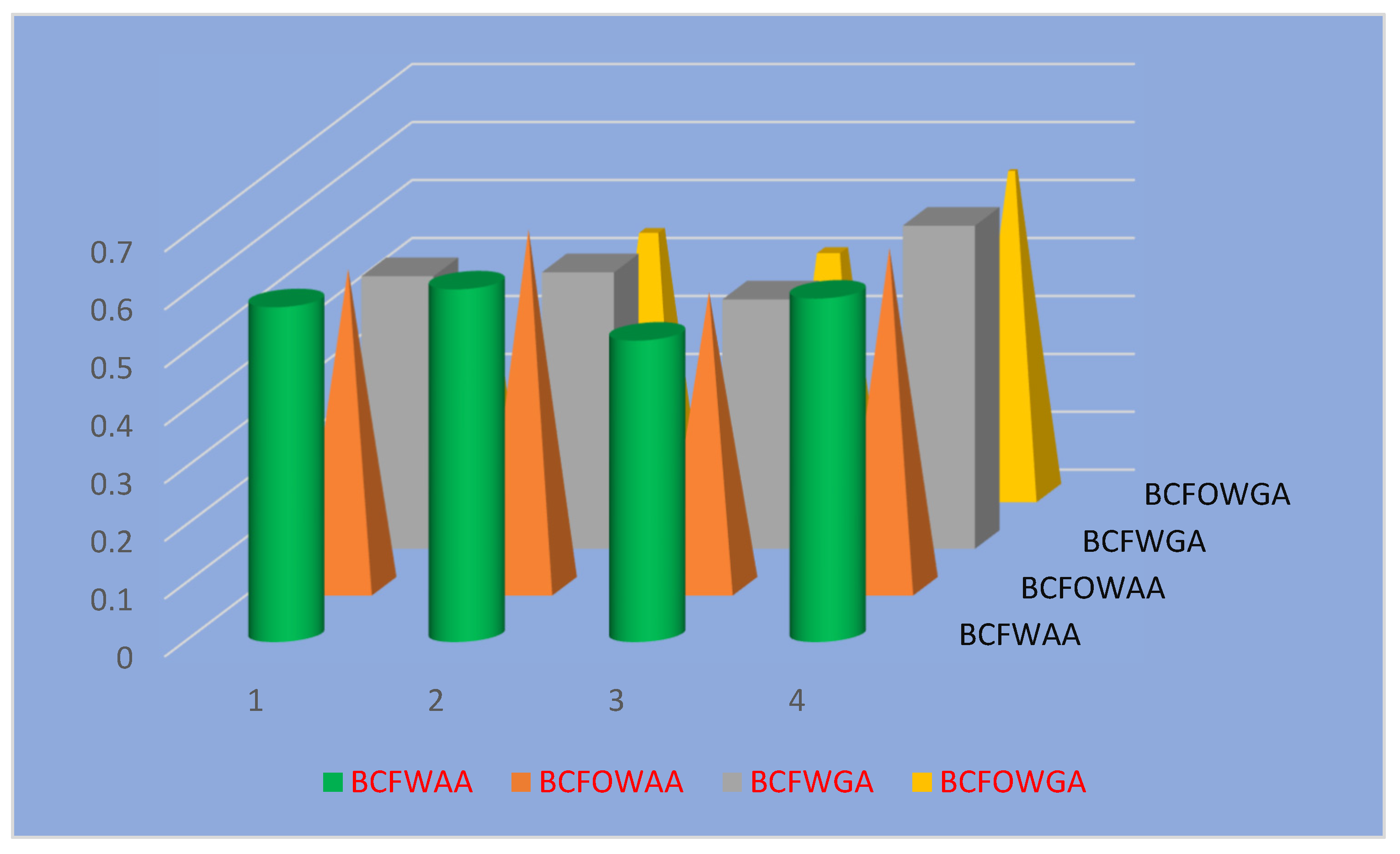
Step 3: Evaluate the SV of the aggregated values, as stated in

Table 3. The score values of the aggregated values given in Table 2.

Operators	${\mathfrak{S}}_{\mathit{S}\mathit{F}}\left({\mathsf{ƀ}}_1\right)$	${\mathfrak{S}}_{\mathit{S}\mathit{F}}\left({\mathsf{ƀ}}_2\right)$	${\mathfrak{S}}_{\mathit{S}\mathit{F}}\left({\mathsf{ƀ}}_3\right)$	${\mathfrak{S}}_{\mathit{S}\mathit{F}}\left({\mathsf{ƀ}}_4\right)$
BCFWAA	0.5789	0.6097	0.5213	0.5938
BCFOWAA	0.549	0.617	0.5089	0.5852
BCFWGA	0.4711	0.4778	0.431	0.5583
BCFOWGA	0.3542	0.4534	0.4192	0.5576

.

Step 4: Evaluate the ranking values based on the obtained SVs and illustrate the best decision, as stated in

Table 4. Ranking values.

Operators	Ranking
BCFWAA Operator	${\mathsf{Ŷ}}_2>{\mathsf{Ŷ}}_4>{\mathsf{Ŷ}}_1>{\mathsf{Ŷ}}_3$
BCFOWAA Operator	${\mathsf{Ŷ}}_2>{\mathsf{Ŷ}}_4>{\mathsf{Ŷ}}_1>{\mathsf{Ŷ}}_3$
BCFWGA Operator	${\mathsf{Ŷ}}_4>{\mathsf{Ŷ}}_2>{\mathsf{Ŷ}}_1>{\mathsf{Ŷ}}_3$
BCFOWGA Operator	${\mathsf{Ŷ}}_4>{\mathsf{Ŷ}}_2>{\mathsf{Ŷ}}_3>{\mathsf{Ŷ}}_1$

. The graphical depiction of the information discussed in Table 3 is illustrated in Figure 3.

The ranking results for any four different types of operators are described in Table 4 using the information of BCFWAA and BCFOWAA operators to get the best optimal value as ${\mathsf{Ŷ}}_2$ and using the information of BCFWGA and BCFOWGA operators get the best optimal value as ${\mathsf{Ŷ}}_4$. To check the supremacy of the diagnosed work, we remove the imaginary part of the diagnosed information, available in

Table 5. Original decision theory contains bipolar fuzzy settings.

	${\mathsf{ƀ}}_{\mathbf{1}}$	${\mathsf{ƀ}}_{\mathbf{2}}$	${\mathsf{ƀ}}_{\mathbf{3}}$	${\mathsf{ƀ}}_{\mathbf{4}}$
${\mathsf{Ŷ}}_1$	$\left(\begin{array}{c}0.11+\iota 0.0, \\ -0.21-\iota 0.0\end{array}\right)$	$\left(\begin{array}{c}0.14+\iota 0.0, \\ -0.16-\iota 0.0\end{array}\right)$	$\left(\begin{array}{c}0.25+\iota 0.0, \\ -0.5-\iota 0.0\end{array}\right)$	$\left(\begin{array}{c}0.55+\iota 0.0, \\ -0.05-\iota 0.0\end{array}\right)$
${\mathsf{Ŷ}}_2$	$\left(\begin{array}{c}0.39+\iota 0.0, \\ -0.35-\iota 0.0\end{array}\right)$	$\left(\begin{array}{c}0.67+\iota 0.0, \\ -0.9-\iota 0.0\end{array}\right)$	$\left(\begin{array}{c}0.89+\iota 0.0, \\ -0.55-\iota 0.0\end{array}\right)$	$\left(\begin{array}{c}0.68+\iota 0.0, \\ -0.5-\iota 0.0\end{array}\right)$
${\mathsf{Ŷ}}_3$	$\left(\begin{array}{c}0.45+\iota 0.0, \\ -0.2-\iota 0.0\end{array}\right)$	$\left(\begin{array}{c}0.23+\iota 0.0, \\ -0.3-\iota 0.0\end{array}\right)$	$\left(\begin{array}{c}0.63+\iota 0.0, \\ -0.67-\iota 0.0\end{array}\right)$	$\left(\begin{array}{c}0.23+\iota 0.0, \\ -0.11-\iota 0.0\end{array}\right)$
${\mathsf{Ŷ}}_4$	$\left(\begin{array}{c}0.26+\iota 0.0, \\ -0.24-\iota 0.0\end{array}\right)$	$\left(\begin{array}{c}0.67+\iota 0.0, \\ -0.43-\iota 0.0\end{array}\right)$	$\left(\begin{array}{c}0.3+\iota 0.0, \\ -0.36-\iota 0.0\end{array}\right)$	$\left(\begin{array}{c}0.5+\iota 0.0, \\ -0.4-\iota 0.0\end{array}\right)$

.

Evaluate the information by using the BCFWAA, BCFOWAA, BCFWGA, and BCFOWGA operators and find the singleton values, as stated in

Table 6. Expression of the aggregated values.

Operators	${\mathsf{ƀ}}_{\mathbf{1}}$	${\mathsf{ƀ}}_{\mathbf{2}}$	${\mathsf{ƀ}}_{\mathbf{3}}$	${\mathsf{ƀ}}_{\mathbf{4}}$
BCFWAA	$\left(\begin{array}{c}0.3408+\iota 0.0, \\ -0.1189-\iota 0.0\end{array}\right)$	$\left(\begin{array}{c}0.6698+\iota 0.0, \\ -0.5623-\iota 0.0\end{array}\right)$	$\left(\begin{array}{c}0.331+\iota 0.0, \\ -0.2007-\iota 0.0\end{array}\right)$	$\left(\begin{array}{c}0.5204+\iota 0.0, \\ -0.3652-\iota 0.0\end{array}\right)$
BCFOWAA	$\left(\begin{array}{c}0.2773+\iota 0.0, \\ -0.34-\iota 0.0\end{array}\right)$	$\left(\begin{array}{c}0.6825+\iota 0.0, \\ -0.582-\iota 0.0\end{array}\right)$	$\left(\begin{array}{c}0.331+\iota 0.0, \\ -0.222-\iota 0.0\end{array}\right)$	$\left(\begin{array}{c}0.4694+\iota 0.0, \\ -0.354-\iota 0.0\end{array}\right)$
BCFWGA	$\left(\begin{array}{c}0.2444+\iota 0.0, \\ -0.1724-\iota 0.0\end{array}\right)$	$\left(\begin{array}{c}0.6223+\iota 0.0, \\ -0.6788-\iota 0.0\end{array}\right)$	$\left(\begin{array}{c}0.2909+\iota 0.0, \\ -0.2659-\iota 0.0\end{array}\right)$	$\left(\begin{array}{c}0.4857+\iota 0.0, \\ -0.3765-\iota 0.0\end{array}\right)$
BCFOWGA	$\left(\begin{array}{c}0.2159+\iota 0.0, \\ -0.3132-\iota 0.0\end{array}\right)$	$\left(\begin{array}{c}0.6038+\iota 0.0, \\ -0.7224-\iota 0.0\end{array}\right)$	$\left(\begin{array}{c}0.2909+\iota 0.0, \\ -0.2833-\iota 0.0\end{array}\right)$	$\left(\begin{array}{c}0.4167+\iota 0.0, \\ -0.3644-\iota 0.0\end{array}\right)$

.

Evaluate the SV of the aggregated values, as stated in

Table 7. Representation of the score values.

Operators	${\mathfrak{S}}_{\mathit{S}\mathit{F}}\left({\mathsf{ƀ}}_1\right)$	${\mathfrak{S}}_{\mathit{S}\mathit{F}}\left({\mathsf{ƀ}}_2\right)$	${\mathfrak{S}}_{\mathit{S}\mathit{F}}\left({\mathsf{ƀ}}_3\right)$	${\mathfrak{S}}_{\mathit{S}\mathit{F}}\left({\mathsf{ƀ}}_4\right)$
BCFWAA	$0.5555$	$0.5269$	$0.5236$	$0.5388$
BCFOWAA	$0.5151$	$0.5252$	$0.5273$	$0.5289$
BCFWGA	$0.518$	$0.4859$	$0.5063$	$0.5273$
BCFOWGA	$0.4757$	$0.4703$	$0.5019$	$0.5131$

.

Evaluate the ranking values based on the obtained SVs and illustrate the best decision, as stated in

Table 8. Ranking values.

Operators	Ranking
BCFWAA Operator	${\mathsf{Ŷ}}_1>{\mathsf{Ŷ}}_4>{\mathsf{Ŷ}}_2>{\mathsf{Ŷ}}_3$
BCFOWAA Operator	${\mathsf{Ŷ}}_4>{\mathsf{Ŷ}}_3>{\mathsf{Ŷ}}_2>{\mathsf{Ŷ}}_1$
BCFWGA Operator	${\mathsf{Ŷ}}_4>{\mathsf{Ŷ}}_1>{\mathsf{Ŷ}}_3>{\mathsf{Ŷ}}_2$
BCFOWGA Operator	${\mathsf{Ŷ}}_4>{\mathsf{Ŷ}}_3>{\mathsf{Ŷ}}_1>{\mathsf{Ŷ}}_2$

.

The ranking results for any four different types of operators are described in Table 8. Using the information of the BCFWAA operator, we get the best optimal value as ${\mathsf{Ŷ}}_1$, and using the information of BCFOWAA, BCFWGA, and BCFOWGA operators, we get the best optimal value as ${\mathsf{Ŷ}}_4$.

4.3. Comparative Analysis

To illustrate the worth and value of the diagnosed operators, we perform a comparison between diagnosed workers and existing operators. That is because the technique of comparison plays a very valuable and meaningful role in the environment of the decision-making technique. The main theme of this theory is comparing the investigated theory with some prevailing theories. For this, we select some existing techniques and try to discuss them here. To enhance the feasibility in the data representation of the evaluation of the attributes and accuracy of decision-making techniques, scholars have developed many techniques using BCFS, for example, Dombi aggregation operators [30] and Hamacher aggregation operators [31]. A comparison of proposed and prevailing scenarios is diagnosed in

Table 9. Comparative analysis of the proposed work.

Authors	Methods	${\mathfrak{S}}_{\mathit{S}\mathit{F}}\left({\mathsf{ƀ}}_1\right)$	${\mathfrak{S}}_{\mathit{S}\mathit{F}}\left({\mathsf{ƀ}}_2\right)$	${\mathfrak{S}}_{\mathit{S}\mathit{F}}\left({\mathsf{ƀ}}_3\right)$	${\mathfrak{S}}_{\mathit{S}\mathit{F}}\left({\mathsf{ƀ}}_4\right)$	Ranking
Mahmood et al. [30]	BCFHWA	0.549	0.617	0.509	0.585	${\mathsf{Ŷ}}_2>{\mathsf{Ŷ}}_4>{\mathsf{Ŷ}}_1>{\mathsf{Ŷ}}_3$
Mahmood et al. [30]	BCFHWG	0.451	0.383	0.491	0.415	${\mathsf{Ŷ}}_3>{\mathsf{Ŷ}}_1>{\mathsf{Ŷ}}_4>{\mathsf{Ŷ}}_1$
Mahmood and Ur Rehman [31]	BCFDWA	0.614	0.683	0.562	0.601	${\mathsf{Ŷ}}_2>{\mathsf{Ŷ}}_1>{\mathsf{Ŷ}}_4>{\mathsf{Ŷ}}_3$
Mahmood and Ur Rehman [31]	BCFDWG	0.37	0.214	0.398	0.36	${\mathsf{Ŷ}}_3>{\mathsf{Ŷ}}_1>{\mathsf{Ŷ}}_4>{\mathsf{Ŷ}}_3$
Proposed	BCFWAA	0.5789	0.6097	0.5213	0.5938	${\mathsf{Ŷ}}_2>{\mathsf{Ŷ}}_4>{\mathsf{Ŷ}}_1>{\mathsf{Ŷ}}_3$
Proposed	BCFOWAA	0.549	0.617	0.5089	0.5852	${\mathsf{Ŷ}}_2>{\mathsf{Ŷ}}_4>{\mathsf{Ŷ}}_1>{\mathsf{Ŷ}}_3$
Proposed	BCFWGA	0.4711	0.4778	0.431	0.5583	${\mathsf{Ŷ}}_4>{\mathsf{Ŷ}}_2>{\mathsf{Ŷ}}_1>{\mathsf{Ŷ}}_3$
Proposed	BCFOWGA	0.3542	0.4534	0.4192	0.5576	${\mathsf{Ŷ}}_4>{\mathsf{Ŷ}}_2>{\mathsf{Ŷ}}_3>{\mathsf{Ŷ}}_1$

, and its graphical depiction is illustrated in Figure 4.

Figure 4 contains different alternatives in the shape of distinct colors, which shows the ranking results. Further, the theory of BCF information is of much value due to its strong shape. In this manuscript, the defined operators are computed based on the algebraic t-norm and t-conorm. From Table 9, we noticed that all prevailing and proposed works give different types of results. In [30,31], experts investigated the idea of Hamacher and Dombi aggregation operators by using the Hamacher t-norm and t-conorm and Dombi t-norm and t-conorm. Many people have diagnosed different types of norms, such as Einstein t-norm and t-conorm and Frank t-norm and t-conorm. In the future, we will try to employ them in the region of BCF information.

The theory of BCF information is a meaningful and valuable framework used for the identification and classification of the problematic and awkward information that happens in genuine life dilemmas.

5. Conclusions

In this manuscript, we combined the theory of BCF information with arithmetic/geometric aggregation operators and diagnosed the theory of CFWAA, BCFOWAA, BCFWGA, and BCFOWGA operators for BCFNs. Further, the fundamental properties and their related results were also examined to show the feasibility and originality of the diagnosed approaches. Moreover, we implemented the diagnosed theory in the field of the MADM tool using BCF settings. Finally, a benchmark dilemma was used for comparison with various prevailing techniques to justify the cogency and dominancy of the evaluated operators.

5.1. Limitations

We noticed that the theory of BCF information is very dominant and valuable, but in various situations, it is not working effectively, for example, if an expert gives information in the form of bipolar complex intuitionistic fuzzy sets, bipolar complex Pythagorean fuzzy sets, bipolar complex picture fuzzy sets, and bipolar complex spherical fuzzy sets.

5.2. Future Work

In the future, the theory of the Maclaurin symmetric mean [32], rough mF bipolar soft environment [33], bipolar fuzzy N-soft sets and their application [34], bipolar soft sets and their application in decision making [35] will be studied, and we will try to utilize them in the environment of BCF information.

References

1. Zadeh, L.A. Fuzzy sets. Inf. Control. 1965, 8, 338–353. [Google Scholar] [CrossRef] [Green Version]
2. Akram, M.; Adeel, A.; Alcantud, J.C.R. Fuzzy N-soft sets: A novel model with applications. J. Intell. Fuzzy Syst. 2018, 35, 4757–4771. [Google Scholar] [CrossRef]
3. Akram, M.; Adeel, A.; Alcantud, J.C.R. Hesitant fuzzy N-soft sets: A new model with applications in decision-making. Intell. Fuzzy Syst. 2019, 36, 6113–6127. [Google Scholar] [CrossRef]
4. Ohlan, R.; Ohlan, A. A bibliometric overview and visualization of fuzzy sets and systems between 2000 and 2018. Ser. Libr. 2022, 81, 190–212. [Google Scholar] [CrossRef]
5. Abdullah, S.; Al-Shomrani, M.M.; Liu, P.; Ahmad, S. A new approach to three-way decisions making based on fractional fuzzy decision-theoretical rough set. Int. J. Intell. Syst. 2022, 37, 2428–2457. [Google Scholar] [CrossRef]
6. Zhang, W.R. Bipolar fuzzy sets and relations: A computational framework for cognitive modeling and multiagent decision analysis. In NAFIPS/IFIS/NASA’94, Proceedings of the First International Joint Conference of The North American Fuzzy Information Processing Society Biannual Conference. The Industrial Fuzzy Control and Intellige, San Antonio, TX, USA, 18–21 December 1994; IEEE: New York, NY, USA, 1994; pp. 305–309. [Google Scholar]
7. Jana, C.; Pal, M.; Wang, J.Q. Bipolar fuzzy Dombi aggregation operators and its application in multiple-attribute decision-making process. J. Ambient Intell. Humaniz. Comput. 2019, 10, 3533–3549. [Google Scholar] [CrossRef]
8. Jana, C.; Pal, M.; Wang, J.Q. Bipolar fuzzy Dombi prioritized aggregation operators in multiple attribute decision making. Soft Comput. 2020, 24, 3631–3646. [Google Scholar] [CrossRef]
9. Mahmood, T. A novel approach towards bipolar soft sets and their applications. J. Math. 2020, 2020, 4690808. [Google Scholar] [CrossRef]
10. Abdullah, S.; Aslam, M.; Ullah, K. Bipolar fuzzy soft sets and its applications in decision making problem. J. Intell. Syst. 2014, 27, 729–742. [Google Scholar] [CrossRef] [Green Version]
11. Riaz, M.; Tehrim, S.T. Cubic bipolar fuzzy ordered weighted geometric aggregation operators and their application using internal and external cubic bipolar fuzzy data. Comput. Appl. Math. 2019, 38, 87. [Google Scholar] [CrossRef]
12. Riaz, M.; Tehrim, S.T. Multi-attribute group decision making based on cubic bipolar fuzzy information using averaging aggregation operators. J. Intell. Fuzzy Syst. 2019, 37, 2473–2494. [Google Scholar] [CrossRef]
13. Jana, C. Multiple attribute group decision-making method based on extended bipolar fuzzy MABAC approach. Comput. Appl. Math. 2021, 40, 227. [Google Scholar] [CrossRef]
14. Yager, R.R.; Rybalov, A. Bipolar aggregation using the Uninorms. Fuzzy Optim. Decis. Mak. 2011, 10, 59–70. [Google Scholar] [CrossRef]
15. Naz, S.; Akram, M.; Al-Shamiri, M.M.A.; Khalaf, M.M.; Yousaf, G. A new MAGDM method with 2-tuple linguistic bipolar fuzzy Heronian mean operators. Math. Biosci. Eng. 2022, 19, 3843–3878. [Google Scholar] [CrossRef]
16. Mesiar, R.; Stupňanová, A.; Jin, L. Bipolar ordered weighted averages: BIOWA operators. Fuzzy Sets Syst. 2022, 433, 108–121. [Google Scholar] [CrossRef]
17. Singh, P.K. Bipolar fuzzy attribute implications. Quantum Mach. Intell. 2022, 4, 4. [Google Scholar] [CrossRef]
18. Gutiérrez, I.; Gómez, D.; Castro, J.; Espínola, R. A new community detection problem based on bipolar fuzzy measures. In Computational Intelligence and Mathematics for Tackling Complex Problems 2; Springer: Cham, Switzerland, 2022; Volume 955, p. 91. ISBN 978-3-030-88817-6. [Google Scholar]
19. Liu, P.; Shen, M.; Pedrycz, W. MAGDM Framework Based on Double Hierarchy Bipolar Hesitant Fuzzy Linguistic Information and Its Application to Optimal Selection of Talents. Int. J. Fuzzy Syst. 2022, 1–23. [Google Scholar] [CrossRef]
20. Mandal, W.A. Bipolar pythagorean fuzzy sets and their application in Multi-attribute decision making problems. Ann. Data Sci. 2021, 4, 1–33. [Google Scholar] [CrossRef]
21. Ramot, D.; Milo, R.; Friedman, M.; Kandel, A. Complex fuzzy sets. IEEE Trans. Fuzzy Syst. 2002, 10, 171–186. [Google Scholar] [CrossRef]
22. Song, H.; Bi, L.; Hu, B.; Xu, Y.; Dai, S. New distance measures between the interval-valued complex fuzzy sets with applications to decision-making. Math. Probl. Eng. 2021, 2021, 6685793. [Google Scholar] [CrossRef]
23. Ahsan, M.; Saeed, M.; Mehmood, A.; Saeed, M.H.; Asad, J. The study of HIV diagnosis using complex fuzzy hypersoft mapping and proposing appropriate treatment. IEEE Access 2021, 9, 104405–104417. [Google Scholar] [CrossRef]
24. Mahmood, T.; Ali, Z.; Gumaei, A. Interdependency of complex fuzzy neighborhood operators and derived complex fuzzy coverings. IEEE Access 2021, 9, 73506–73521. [Google Scholar] [CrossRef]
25. Alolaiyan, H.; Alshehri, H.A.; Mateen, M.H.; Pamucar, D.; Gulzar, M. A novel algebraic structure of (α, β)-complex fuzzy subgroups. Entropy 2021, 23, 992. [Google Scholar] [CrossRef] [PubMed]
26. Liu, P.; Ali, Z.; Mahmood, T. The distance measures and cross-entropy based on complex fuzzy sets and their application in decision making. J. Intell. Fuzzy Syst. 2020, 39, 3351–3374. [Google Scholar] [CrossRef]
27. Bi, L.; Zeng, Z.; Hu, B.; Dai, S. Two classes of entropy measures for complex fuzzy sets. Mathematics 2019, 7, 96. [Google Scholar] [CrossRef] [Green Version]
28. Dai, S.; Bi, L.; Hu, B. Distance measures between the interval-valued complex fuzzy sets. Mathematics 2019, 7, 549. [Google Scholar] [CrossRef] [Green Version]
29. Mahmood, T.; Ur Rehman, U. A novel approach towards bipolar complex fuzzy sets and their applications in generalized similarity measures. Int. J. Intell. Syst. 2022, 37, 535–567. [Google Scholar] [CrossRef]
30. Mahmood, T.; Ur Rehman, U.; Ahmmad, J.; Santos-García, G. Bipolar Complex Fuzzy Hamacher Aggregation Operators and Their Applications in Multi-Attribute Decision Making. Mathematics 2022, 10, 23. [Google Scholar] [CrossRef]
31. Mahmood, T.; Ur Rehman, U. A method to multi-attribute decision making technique based on Dombi aggregation operators under bipolar complex fuzzy information. Comput. Appl. Math. 2022, 41, 47. [Google Scholar] [CrossRef]
32. Ullah, K. Picture fuzzy Maclaurin symmetric mean operators and their applications in solving multiattribute decision-making problems. Math. Probl. Eng. 2021, 2021, 1098631. [Google Scholar] [CrossRef]
33. Akram, M.; Ali, G.; Shabir, M. A hybrid decision-making framework using rough mF bipolar soft environment. Granul. Comput. 2021, 6, 539–555. [Google Scholar] [CrossRef]
34. Akram, M.; Amjad, U.; Davvaz, B. Decision-making analysis based on bipolar fuzzy N-soft information. Comput. Appl. Math. 2021, 40, 182. [Google Scholar] [CrossRef]
35. Karaaslan, F.; Karataş, S. A new approach to bipolar soft sets and its applications. Discret. Math. Algorithms Appl. 2015, 7, 1550054. [Google Scholar] [CrossRef] [Green Version]
Figure 1. The geometrical shape of the existing theory.
Mathematics 10 01726 g001
Figure 2. The geometrical shape of the proposed theory.
Mathematics 10 01726 g002
Figure 3. A graphical depiction of the information discussed in Table 3.
Mathematics 10 01726 g003
Figure 4. A graphical depiction comparison among proposed and prevailing scenarios. Where, BCFHWA, BCFHWG are presented by Mahmood et al. [30] and BCFDWA, BCFDWG are presented by Mahmood and Ur Rehman [31].
Mathematics 10 01726 g004