Complex Dynamic Behaviour of Food Web Model with Generalized Fractional Operator

Abstract

We apply a new generalized Caputo operator to investigate the dynamical behaviour of the non-integer food web model (FWM). This dynamical model has three population species and is nonlinear. Three types of species are considered in this population: prey species, intermediate predators, and top predators, and the top predators are also divided into mature and immature predators. We calculated the uniqueness and existence of the solutions applying the fixed-point hypothesis. Our study examines the possibility of obtaining new dynamical phase portraits with the new generalized Caputo operator and demonstrates the portraits for several values of fractional order. A generalized predictor–corrector (P-C) approach is utilized in numerically solving this food web model. In the case of the nonlinear equations system, the effectiveness of the used scheme is highly evident and easy to implement. In addition, stability analysis was conducted for this numerical scheme.

1. Introduction

Energy and materials follow one path between species in a food chain model, whereas food webs are more complex because they connect many food chains. Different trophic levels are found in a food web. There are various categories of organisms within the trophic levels, including producers, consumers, and decomposers. The structure of a food web is typically represented by a lattice arrangement. Using a system of differential equations, it is possible to design food chains and food webs. Food chains, in ecology, are a chain of organisms feeding on the organism next to them, while food webs are a collection of food chains joined together. It has been of interest to several researchers to analyse the dynamical behaviour of the food chain model and the web model [1,2,3,4]. A modular food web theory, which studies the structural and functional properties of low-species-based food webs, aims to determine how the structure and interactions mediate ecosystem stability [5,6]. Several species in nature have life cycles that are divided into at least two stages: mature and immature. These stages have different characteristics. Food web models (FWMs) depicting a stage structure have been extensively studied [7,8]. The impact of cannibalism on ecological systems has been studied extensively over the past few decades. Aquatic, as well as terrestrial food webs have cannibalistic populations. This subject has been addressed by several studies [9,10,11,12]. Stage-structured populations frequently engage in cannibalism, whether in the wild or in watery food webs. The cannibalism model was examined and investigated by Diekmann et al. [13]. A watery food chain in which a predator cannibalizes was studied by Bhattacharyya and Pal [14]. The dynamics of the system are therefore influenced by cannibalism in a very significant way. Fishes, birds, mammals, and others are among the animals that have cannibalistic natures.

There are over 300 years of development behind fractional calculus, and today, this is still an important concept of studying real-world problems [15,16,17,18,19,20]. The literature of fractional calculus has introduced a variety of fractional derivatives, including Caputo [21], Atangana–Baleanu [22], and Caputo–Fabrizio [23], which are the most widely used derivatives. Fractional differential equations can describe dynamic processes within biological and ecological systems with a higher degree of accuracy and reliability since most biological and ecological mathematical models have long-term memories. An understanding of fractional species systems can provide new possibilities for describing the dynamic behaviours of multi-species food web ecosystems, given the complexity and existence of nonlinear effects [24]. In addition, fractional-order forms have a number of advantages, such as a meticulous illustration and an accurate interpretation of operation rules. In order to further explore the dynamics of systems with competition, predation, and parasitism, classical integer differential equations of ecosystems are replaced with fractional differential equations. The literature contains a variety of nonlocal operators, which are used extensively in applied mathematics. An integral and fractional derivative introduced by Katugampola in 2014 generalizes both Riemann–Liouville and Hadamard integrals and derivatives [25,26]. The generalized Caputo operator was recently constructed by Odibat et al. [27]. In the literature, the generalized Caputo operator has been applied in various ways. A recent study by Rubayyi T. Alqahtani et al. [28] utilized a generalized Caputo operator to model bioethanol production. The new generalized Caputo operator was used to analyse the COVID-19 model [29]. In the paper [30], the author investigated irregular meshes with finite difference methods to determine the error estimates when the Caputo operator of the solution of the FDEs has a low smoothness. The paper [31] developed the asymptotic expansion formula for the trapezoidal approximation of the fractional integral, and the author applied the expansion formula to calculate approximations for fractional integrals of orders $\alpha ,\alpha +1,\alpha +2,\alpha +3,$ and $\alpha +4$.

In this paper, we extend the classical integer-order food web model (FWM) to a non-integer food web model through a generalized Caputo operator. Moreover, we discuss a generalized predictor–corrector numerical solution that is a generalization of the P-C numerical scheme [32,33] to study the complexity of the food web model’s behaviour, and we analyse the stability of this scheme. With the generalized Caputo operator, a non-uniform grid is used in the P-C scheme instead of the uniform grid in the Caputo operator. $\phi$ and $\rho$ are the only parameters needed to generalize the Caputo integral operator, which provides a great deal of theoretical and numerical equipment for fractional mathematical modelling. There are numerous applications of this P-C technique in various fields of FDEs. In this study, we analysed the behaviour of the food web model on various different fractional orders and on another parameter of the derivative, which gives us different dynamic phase diagrams of this food web model.

Due to Caputo derivatives describing better certain physical problems involving memory effects, we defined the generalized fractional derivatives in a Caputo form. This Caputo version of generalized fractional derivatives would prove useful for researchers interested in describing real-world phenomena using fractional operators. Finally, by noticing that ${lim}_{\rho \to 0}\left(\frac{x^{\rho }-a^{\rho }}{\rho }\right)=In\left(\frac{x}{a}\right)$ and ${lim}_{\rho \to 0}\left(\frac{b^{\rho }-x^{\rho }}{\rho }\right)=In\left(\frac{b}{x}\right)$ lead to Hadamard and Caputo–Hadamard results, we saw that the limiting case as $\rho \to 0$ leads to those results. Furthermore, when $\rho \to 1$, the fractional derivatives of Riemann–Liouville and of Caputo were obtained.

Outline of the Paper

We divided this whole work into the following sections: Section 2 represents the description of the food web model. The preliminaries of fractional calculus (FC) are covered in Section 3. The existence of solutions is demonstrated in Section 4. Solution uniqueness is demonstrated in Section 5. Section 6 presents generalized predictor–corrector numerical algorithms for fractional-order food web models using the generalized Caputo operator. Section 7 contains simulations and discussions of the numerical results. A conclusion is given in Section 8.

2. Description of the Food Web Model

Our study proposes and analyses a three-species FWM that includes cannibalism and a stage structure within top predator species. Predators at the top are generally divided into immature and mature stages. Initial stage individuals are unable to hunt or reproduce, as they are dependent on their mature parents for survival. Additionally, we constructed an ecological model that includes stage cannibalism and structure in the top predators as part of a three-species food web model.

A food web model can be constructed using the above considerations [34].

$$\begin{array}{ccc}\hfill \frac{dx\left(t\right)}{dt}& =& rx\left(t\right)\left(1-\frac{x\left(t\right)}{\mathcal{H}}\right)-a_{1}x\left(t\right)y\left(t\right),\hfill \\ \hfill \frac{dy\left(t\right)}{dt}& =& a_1{e}_{1}x\left(t\right)y\left(t\right)-a_{2}y\left(t\right)z\left(t\right)-d_{1}y\left(t\right),\hfill \\ \hfill \frac{dz\left(t\right)}{dt}& =& a_2{e}_{2}y\left(t\right)z\left(t\right)+a_3{e}_{3}z\left(t\right)u\left(t\right)+cu\left(t\right)-d_{2}z\left(t\right),\hfill \\ \hfill \frac{du\left(t\right)}{dt}& =& bz\left(t\right)-cu\left(t\right)-a_{3}z\left(t\right)u\left(t\right)-d_{3}u\left(t\right).\hfill \end{array}$$

(1)

Prey density (lower level species) at time t is denoted by x(t); intermediate predator density (middle-level species) at time t is denoted by y(t); top predator density (mature and immature of higher-level species) at time t is denoted by z(t), u(t). With an intrinsic growth rate r and carrying capacity $\mathcal{H}$, the prey grows logistically. Based on the Lotka–Volterra functional response, the intermediate predator consumes the prey at the lowest level, with an attack rate $a_1$ and a conversion rate $e_1$. In the absence of their food source, it continues to decay exponentially as a result of natural mortality rate $d_1$. There are two kinds of top predators: mature and immature. Immature populations are assumed to grow exponentially along with their parents denoted by the mature population with growth rate b, while a part grows up to become a mature population with growth rate c. Additionally, both the mature and immature populations face natural death with mortality rates of $d_2$ and $d_3$, respectively. With maximum attack rate $a_3$ and conversion rate $e_2$, the mature top predator attacks the intermediate predator using the Lotka–Volterra response functional. When the availability of their preferred food becomes rare, they cannibalise the immature top predator based on the Lotka–Volterra functional response with maximum attack rate $a_3$ and conversion rate $e_3$.

Equilibrium Points of the Food Web Model

In the part of this section, we calculate the equilibrium points corresponding to the food web model. The steady-state conditions for the model are as follows:

• ${\mathbf{E}}_0=(0,0,0,0)$ is the trivial equilibrium point that always exists.
• ${\mathbf{E}}_1=(\mathcal{H},0,0,0)$ is the axial equilibrium point.
• ${\mathbf{E}}_2=(\check{x},\check{y},0,0)=\left(\frac{d_1}{a_1{e}_1},\frac{r}{a_1}\left(1-\frac{d_1}{a_1{e}_1\mathcal{H}}\right),0,0\right)$ is the top predator free equilibrium point. If the condition $\mathcal{H}>\frac{d_1}{a_1{e}_1}$ holds, then it exists.
• ${\mathbf{E}}_3=(\ddot{x},\ddot{y},\ddot{z},\ddot{u})=\left(\ddot{x},\frac{r}{a_1}\left(1-\frac{\ddot{x}}{\mathcal{H}}\right),\frac{a_1{e}_1\ddot{x}-d_1}{a_2},\frac{b(a_1{e}_1\ddot{x}-d_1)}{a_2(c+d_3)+a_3(a_1{e}_1\ddot{x}-d_1)}\right)$ is the interior equilibrium point. The characteristic equation for $\ddot{x}$ is as follows:

  $$\begin{array}{c}\hfill {\gamma }_1{\ddot{x}}^3+{\gamma }_2{\ddot{x}}^2+{\gamma }_3\ddot{x}+{\gamma }_4=0.\end{array}$$

  (2)

  where

  $$\begin{array}{ccc}\hfill {\gamma }_1& =& -a_1^2{a}_2{a}_3{e}_1^2{e}_{2}r<0.\hfill \\ \hfill {\gamma }_2& =& a_1{e}_1[a_2{e}_{2}r(d_1{a}_3-a_2(c+d_3))+a_1^2{a}_3{e}_1\mathcal{H}(b{e}_3-d_2)+a_2{a}_{3}r(a_1{e}_1{e}_2\mathcal{H}+d_1)]\hfill \\ \hfill {\gamma }_3& =& a_2^{2}r(c+d_3)(a_1{e}_1{e}_2\mathcal{H}+2d_1)-2\mathcal{H}{a}_1{a}_3{e}_1{d}_1(r{a}_2{e}_2-a_1{d}_2)\hfill \\ & -& \mathcal{H}{e}_1{a}_1^2{a}_2(d_2{d}_3+c(d_2-b))-b\mathcal{H}{e}_1{a}_1^2{d}_1(a_3{e}_3+1)-r{a}_2{a}_3{d}_1.\hfill \\ \hfill {\gamma }_4& =& r\mathcal{H}{a}_2{e}_2{d}_1(a_3{d}_1-a_2(c+d_3))+\mathcal{H}{a}_1{a}_3{d}_1^2(b{e}_3-d_2)+\mathcal{H}{a}_1{d}_1(a_2{d}_2(c+d_3)-bc).\hfill \end{array}$$
  Thus, a simple computation shows that this exists only if and only if the following is true:

  $$\begin{array}{c}\hfill \check{x}<\ddot{x}<\mathcal{H},\end{array}$$

  (3)

  with one set condition $({\gamma }_2<0$ and ${\gamma }_4<0)$ or $({\gamma }_3>0$ and ${\gamma }_4>0)$.

3. Preliminaries

Definition 1.

The non-integer-order Riemann–Liouville (RL) integral of a function f(t) is described as

$$\begin{array}{ccc}\hfill {}_a^{RL}{\mathcal{I}}_t^{\phi }\left[f\left(t\right)\right]& =& {\displaystyle \frac{1}{\Gamma \left(\phi \right)}}{\int }_a^{t}f\left(\varsigma \right){(t-\varsigma )}^{\phi -1}d\varsigma .\hfill \\ \hfill {}_a^{RL}{\mathcal{I}}_t^0\left[f\left(t\right)\right]& =& f\left(t\right).\hfill \end{array}$$

(4)

Definition 2.

Consider $f\left(t\right)$∈$H^1$ to be a differentiable function in the interval $(a,b),a<b,$ and $\phi \in [0,1]$, then we define the Caputo non-classical operator as

$$\begin{array}{c}\hfill {}_a^C{\mathcal{D}}_t^{\phi }f\left(t\right)=\left\{\begin{array}{ccc}\frac{1}{\Gamma (n-\phi )}{\int }_a^t{f}^{\left(n\right)}\left(\varsigma \right){(t-\varsigma )}^{(n-\phi -1)}d\varsigma ,\hfill & if\hfill & n-1<\phi <n,\hfill \\ \frac{d^{n}f\left(t\right)}{d{t}^n},\hfill & if\hfill & \phi =n,\hfill \end{array}\right.\end{array}$$

(5)

Gamma functions are represented by $\Gamma (.)$. Here is the definition of the gamma function:

$$\begin{array}{c}\hfill \Gamma \left(x\right)={\int }_0^{+\infty }{\Omega }^{x-1}{e}^{-\Omega }d\Omega ,(Re\left(x\right)>0).\end{array}$$

(6)

Definition 3.

Here, the order of derivative $\phi >0$ and $\rho >0$, and the generalized non-classical integral ${}_{}^{GC}{\mathcal{I}}_{a+}^{\phi ,\rho }$ of a function f(t) is defined (assuming it exists) as

$${}_{}^{GC}{\mathcal{I}}_{a+}^{\phi ,\rho }\left[f\left(t\right)\right]=\frac{{\rho }^{1-\phi }}{\Gamma \left(\phi \right)}{\int }_a^t{\varsigma }^{\rho -1}f\left(\varsigma \right){(t^{\rho }-{\varsigma }^{\rho })}^{\phi -1}d\varsigma ,t>a.$$

(7)

Definition 4.

Here, the order of derivative $\phi >0$ $(m-1<\phi <m)$ and $\rho >0$. For a function f(t), the generalized Riemann-type non-classical derivative ${}_{}^{GRL}{\mathcal{D}}_{a+}^{\phi ,\rho }$ is defined as

$${}_{}^{GRL}{\mathcal{D}}_{a+}^{\phi ,\rho }\left[f\left(t\right)\right]=\frac{{\rho }^{\phi -m+1}}{\Gamma (m-\phi )}\left(t^{1-\rho }\frac{d}{dt}\right){\int }_a^t{\varsigma }^{\rho -1}f\left(\varsigma \right){(t^{\rho }-{\varsigma }^{\rho })}^{\phi -1}d\varsigma ,t>a\ge 0.$$

(8)

Definition 5.

Here, the order of derivative $\phi >0$, $\rho >0$ and $m=\lceil \phi \rceil$. For a function f(t), the generalized Caputo-type non-classical derivative ${}_{}^{GC}{\mathcal{D}}_{a+}^{\phi ,\rho }$ is defined as

$${}_{}^{GC}{\mathcal{D}}_{a+}^{\phi ,\rho }\left[f\left(t\right)\right]=\left({}_{}^{GRL}{\mathcal{D}}_{a+}^{\phi ,\rho }\left[f\left(x\right)-\sum _{n=0}^{m-1}\frac{f\left(n\right)\left(a\right)}{n!}{(x-a)}^n\right]\right)\left(t\right),t>a\ge 0.$$

(9)

Definition 6.

Here, the order of derivative $\phi >0$ $(m-1<\phi <m)$ and $\rho >0$. For a function f(t), the generalized Caputo-type non-classical derivative ${}_{}^{GC}{\mathcal{D}}_{a+}^{\phi ,\rho }$ is defined as

$${}_{}^{GC}{\mathcal{D}}_{a+}^{\phi ,\rho }\left[f\left(t\right)\right]=\frac{{\rho }^{\phi -m+1}}{\Gamma (m-\phi )}{\int }_a^t{\varsigma }^{\rho -1}f\left(\varsigma \right){(t^{\rho }-{\varsigma }^{\rho })}^{\phi -1}\left({\varsigma }^{1-\rho }\frac{d}{d\varsigma }\right)d\varsigma ,t>a\ge 0.$$

(10)

• The relation between the Riemann–Liouville and the generalized non-classical integral from the substitution ${\chi }^{\rho }\to \chi$ is as follows

  $${}_a^{GC}{\mathcal{I}}_t^{\phi ,\rho }\left[f\left(t\right)\right]={\rho }^{-\phi }{}_{a^{\rho }}^{RL}{\mathcal{I}}_{t^{\rho }}^{\phi }\left[f\left(t^{1/\rho }\right)\right].$$

  (11)

When the lower limit is zero $a=0$, the relation is

$${}_0^{GC}{\mathcal{I}}_t^{\phi ,\rho }\left[f\left(t\right)\right]={\rho }^{-\phi }{}_0^{RL}{\mathcal{I}}_{t^{\rho }}^{\phi }\left[f\left(t^{1/\rho }\right)\right].$$

(12)

4. Existence of Solutions

The fixed-point assumption is used to investigate the existence of a solution for the fractional food web mathematical model. Now, a non-integer food web mathematical model can be described as follows.

$$\begin{array}{ccc}\hfill {}_{}^{GC}{\mathcal{D}}_{0+}^{\phi ,\rho }\left[x\left(t\right)\right]& =& rx\left(t\right)\left(1-\frac{x\left(t\right)}{\mathcal{H}}\right)-a_{1}x\left(t\right)y\left(t\right),\hfill \\ \hfill {}_{}^{GC}{\mathcal{D}}_{0+}^{\phi ,\rho }\left[y\left(t\right)\right]& =& a_1{e}_{1}x\left(t\right)y\left(t\right)-a_{2}y\left(t\right)z\left(t\right)-d_{1}y\left(t\right),\hfill \\ \hfill {}_{}^{GC}{\mathcal{D}}_{0+}^{\phi ,\rho }\left[z\left(t\right)\right]& =& a_2{e}_{2}y\left(t\right)z\left(t\right)+a_3{e}_{3}z\left(t\right)u\left(t\right)+cu\left(t\right)-d_{2}z\left(t\right),\hfill \\ \hfill {}_{}^{GC}{\mathcal{D}}_{0+}^{\phi ,\rho }\left[u\left(t\right)\right]& =& bz\left(t\right)-cu\left(t\right)-a_{3}z\left(t\right)u\left(t\right)-d_{3}u\left(t\right).\hfill \end{array}$$

(13)

The initial conditions of a mathematical model of a food web are as follows:

$$\begin{array}{c}\hfill x\left(0\right)=x_0,y\left(0\right)=y_0,z\left(0\right)=z_0,u\left(0\right)=u_0.\end{array}$$

(14)

Using the generalized Caputo-type non-classical integral, we have

$$\begin{array}{c}\hfill \begin{array}{ccc}\hfill x\left(t\right)& -& x\left(0\right)={\displaystyle \frac{{\rho }^{1-\phi }}{\Gamma \left(\phi \right)}}{\int }_0^t\left\{rx\left(t\right)\left(1-{\displaystyle \frac{x\left(t\right)}{\mathcal{H}}}\right)-a_{1}x\left(t\right)y\left(t\right)\right\}{\varsigma }^{\rho -1}{(t^{\rho }-{\varsigma }^{\rho })}^{(\phi -1)}d\varsigma ,\hfill \\ \hfill y\left(t\right)& -& y\left(0\right)={\displaystyle \frac{{\rho }^{1-\phi }}{\Gamma \left(\phi \right)}}{\int }_0^t\left\{a_1{e}_{1}x\left(t\right)y\left(t\right)-a_{2}y\left(t\right)z\left(t\right)-d_{1}y\left(t\right)\right\}{\varsigma }^{\rho -1}{(t^{\rho }-{\varsigma }^{\rho })}^{(\phi -1)}d\varsigma ,\hfill \\ \hfill z\left(t\right)& -& z\left(0\right)={\displaystyle \frac{{\rho }^{1-\phi }}{\Gamma \left(\phi \right)}}{\int }_0^t\left\{a_2{e}_{2}y\left(t\right)z\left(t\right)+a_3{e}_{3}z\left(t\right)u\left(t\right)+cu\left(t\right)-d_{2}z\left(t\right)\right\}{\varsigma }^{\rho -1}{(t^{\rho }-{\varsigma }^{\rho })}^{(\phi -1)}d\varsigma ,\hfill \\ \hfill u\left(t\right)& -& u\left(0\right)={\displaystyle \frac{{\rho }^{1-\phi }}{\Gamma \left(\phi \right)}}{\int }_0^t\left\{bz\left(t\right)-cu\left(t\right)-a_{3}z\left(t\right)u\left(t\right)-d_{3}u\left(t\right)\right\}{\varsigma }^{\rho -1}{(t^{\rho }-{\varsigma }^{\rho })}^{(\phi -1)}d\varsigma .\hfill \end{array}\end{array}$$

(15)

In order to simplify, we determine

$$\begin{array}{ccc}\hfill {\mho }_1(t,x)& =& rx\left(t\right)\left(1-\frac{x\left(t\right)}{\mathcal{H}}\right)-a_{1}x\left(t\right)y\left(t\right),\hfill \\ \hfill {\mho }_2(t,y)& =& a_1{e}_{1}x\left(t\right)y\left(t\right)-a_{2}y\left(t\right)z\left(t\right)-d_{1}y\left(t\right),\hfill \\ \hfill {\mho }_3(t,z)& =& a_2{e}_{2}y\left(t\right)z\left(t\right)+a_3{e}_{3}z\left(t\right)u\left(t\right)+cu\left(t\right)-d_{2}z\left(t\right),\hfill \\ \hfill {\mho }_4(t,u)& =& bz\left(t\right)-cu\left(t\right)-a_{3}z\left(t\right)u\left(t\right)-d_{3}u\left(t\right).\hfill \end{array}$$

(16)

Theorem 1.

When $0\le {\mho }_1,{\mho }_2,{\mho }_3,{\mho }_4<1$, then the kernels ${\mho }_l,{\mho }_2,{\mho }_3,{\mho }_4$ satisfy the Lipschitz condition.

Proof of Theorem 1. 

Then, if ${\mho }_1(t,x)=rx\left(t\right)\left(1-\frac{x\left(t\right)}{k}\right)-a_{1}x\left(t\right)y\left(t\right)$ is the kernel and $x\left(t\right)$ and $x_1\left(t\right)$ are two function, we can find

$$\begin{array}{c}\hfill \begin{array}{ccc}\hfill \parallel {\mho }_1(t,x)-{\mho }_1(t,x_1)\parallel & =& ∥rx\left(t\right)\left(1-{\displaystyle \frac{x\left(t\right)}{\mathcal{H}}}\right)-a_{1}x\left(t\right)y\left(t\right)-\left(rx\left(t\right)\left(1-\frac{x\left(t\right)}{\mathcal{H}}\right)-a_{1}x\left(t\right)y\left(t\right)\right)∥,\hfill \\ & =& ∥\left(r\left(1-{\displaystyle \frac{x\left(t\right)+x_1\left(t\right)}{\mathcal{H}}}\right)-a_{1}y\left(t\right)\right)\left(x\left(t\right)-x_1\left(t\right)\right)∥,\hfill \\ & \le & ∥r\left(1-{\displaystyle \frac{x\left(t\right)+x_1\left(t\right)}{\mathcal{H}}}\right)-a_{1}y\left(t\right)∥\parallel x\left(t\right)-x_1\left(t\right)\parallel ,\hfill \\ & \le & \left(r\left(1-{\displaystyle \frac{\parallel x\left(t\right)\parallel +\parallel x_1\left(t\right)\parallel }{k}}\right)-a_1\parallel y\left(t\right)\parallel \right)\parallel x\left(t\right)-x_1\left(t\right)\parallel ,\hfill \\ & \le & \left(r\left(1-{\displaystyle \frac{2q_1}{\mathcal{H}}}\right)-a_1{q}_2\right)\parallel x\left(t\right)-x_1\left(t\right)\parallel ,\hfill \\ & \le & {⨿}_1\parallel x\left(t\right)-x_1\left(t\right)\parallel .\hfill \end{array}\end{array}$$

(17)

By putting ${⨿}_1=\left(r\left(1-\frac{2q_1}{\mathcal{H}}\right)-a_1{q}_2\right)$, $\parallel x\left(t\right)\parallel \le q_1$, $\parallel y\left(t\right)\parallel \le q_2$, $\parallel z\left(t\right)\parallel \le q_3$, and $\parallel u\left(t\right)\parallel \le q_4$ are the bounded functions; furthermore, we have □

$$\begin{array}{c}\hfill \parallel {\mho }_1(t,x)-{\mho }_1(t,x_1)\parallel \le {⨿}_1\parallel x\left(t\right)-x_1\left(t\right)\parallel .\end{array}$$

(18)

Therefore, the Lipschitz condition holds for ${\mho }_1$ if the inequality $0\le {\mho }_1<1$ is the contraction of ${\mho }_1$. As we apply the same procedure to kernels ${\mho }_2$, ${\mho }_3$, and ${\mho }_4$, the following results emerge:

$$\begin{array}{c}\hfill \parallel {\mho }_2(t,y)-{\mho }_2(t,y_1)\parallel \le {⨿}_2\parallel y\left(t\right)-y_1\left(t\right)\parallel ,\\ \hfill \parallel {\mho }_3(t,z)-{\mho }_3(t,z_1)\parallel \le {⨿}_3\parallel z\left(t\right)-z_1\left(t\right)\parallel ,\\ \hfill \parallel {\mho }_4(t,u)-{\mho }_4(t,u_1)\parallel \le {⨿}_4\parallel u\left(t\right)-u_1\left(t\right)\parallel .\end{array}$$

(19)

Kernels ${\mho }_1$, ${\mho }_2$, ${\mho }_3$, and ${\mho }_4$ are determined by Equation (16). Afterwards, we determine the associated integrals:

$$\begin{array}{c}\hfill \begin{array}{ccc}\hfill x\left(t\right)& =& x\left(0\right)+{\displaystyle \frac{{\rho }^{1-\phi }}{\Gamma \left(\phi \right)}}{\int }_0^t{\mho }_1(\varsigma ,x){\varsigma }^{\rho -1}{(t^{\rho }-{\varsigma }^{\rho })}^{(\phi -1)}d\varsigma ,\hfill \\ \hfill y\left(t\right)& =& y\left(0\right)+{\displaystyle \frac{{\rho }^{1-\phi }}{\Gamma \left(\phi \right)}}{\int }_0^t{\mho }_2(\varsigma ,y){\varsigma }^{\rho -1}{(t^{\rho }-{\varsigma }^{\rho })}^{(\phi -1)}d\varsigma ,\hfill \\ \hfill z\left(t\right)& =& z\left(0\right)+{\displaystyle \frac{{\rho }^{1-\phi }}{\Gamma \left(\phi \right)}}{\int }_0^t{\mho }_3(\varsigma ,z){\varsigma }^{\rho -1}{(t^{\rho }-{\varsigma }^{\rho })}^{(\phi -1)}d\varsigma ,\hfill \\ \hfill u\left(t\right)& =& u\left(0\right)+{\displaystyle \frac{{\rho }^{1-\phi }}{\Gamma \left(\phi \right)}}{\int }_0^t{\mho }_4(\varsigma ,u){\varsigma }^{\rho -1}{(t^{\rho }-{\varsigma }^{\rho })}^{(\phi -1)}d\varsigma ;\hfill \end{array}\end{array}$$

(20)

furthermore, we obtain

$$\begin{array}{c}\hfill \begin{array}{ccc}\hfill x_n\left(t\right)& =& x\left(0\right)+{\displaystyle \frac{{\rho }^{1-\phi }}{\Gamma \left(\phi \right)}}{\int }_0^t{\mho }_1(\varsigma ,x_{n-1}){\varsigma }^{\rho -1}{(t^{\rho }-{\varsigma }^{\rho })}^{(\phi -1)}d\varsigma ,\hfill \\ \hfill y_n\left(t\right)& =& y\left(0\right)+{\displaystyle \frac{{\rho }^{1-\phi }}{\Gamma \left(\phi \right)}}{\int }_0^t{\mho }_2(\varsigma ,y_{n-1}){\varsigma }^{\rho -1}{(t^{\rho }-{\varsigma }^{\rho })}^{(\phi -1)}d\varsigma ,\hfill \\ \hfill z_n\left(t\right)& =& z\left(0\right)+{\displaystyle \frac{{\rho }^{1-\phi }}{\Gamma \left(\phi \right)}}{\int }_0^t{\mho }_3(\varsigma ,z_{n-1}){\varsigma }^{\rho -1}{(t^{\rho }-{\varsigma }^{\rho })}^{(\phi -1)}d\varsigma ,\hfill \\ \hfill u_n\left(t\right)& =& u\left(0\right)+{\displaystyle \frac{{\rho }^{1-\phi }}{\Gamma \left(\phi \right)}}{\int }_0^t{\mho }_4(\varsigma ,u_{n-1}){\varsigma }^{\rho -1}{(t^{\rho }-{\varsigma }^{\rho })}^{(\phi -1)}d\varsigma ,\hfill \end{array}\end{array}$$

(21)

and the initial condition is

$$\begin{array}{c}\hfill x\left(0\right)=x_0,y\left(0\right)=y_0,z\left(0\right)=z_0,u\left(0\right)=u_0.\end{array}$$

(22)

When we subtract consecutive terms, we obtain

$$\begin{array}{c}\hfill \begin{array}{ccc}\hfill {\Xi }_n\left(t\right)=x_n\left(t\right)-x_{n-1}\left(t\right)& =& {\displaystyle \frac{{\rho }^{1-\phi }}{\Gamma \left(\phi \right)}}{\int }_0^t({\mho }_1(\varsigma ,x_{n-1})-{\mho }_1(\varsigma ,x_{n-2})){\varsigma }^{\rho -1}{(t^{\rho }-{\varsigma }^{\rho })}^{(\phi -1)}d\varsigma ,\hfill \\ \hfill {\Delta }_n\left(t\right)=y_n\left(t\right)-y_{n-1}\left(t\right)& =& {\displaystyle \frac{{\rho }^{1-\phi }}{\Gamma \left(\phi \right)}}{\int }_0^t({\mho }_2(\varsigma ,y_{n-1})-{\mho }_2(\varsigma ,y_{n-2})){\varsigma }^{\rho -1}{(t^{\rho }-{\varsigma }^{\rho })}^{(\phi -1)}d\varsigma ,\hfill \\ \hfill {\aleph }_n\left(t\right)=z_n\left(t\right)-z_{n-1}\left(t\right)& =& {\displaystyle \frac{{\rho }^{1-\phi }}{\Gamma \left(\phi \right)}}{\int }_0^t({\mho }_3(\varsigma ,z_{n-1})-{\mho }_3(\varsigma ,z_{n-2})){\varsigma }^{\rho -1}{(t^{\rho }-{\varsigma }^{\rho })}^{(\phi -1)}d\varsigma ,\hfill \\ \hfill {\gimel }_n\left(t\right)=u_n\left(t\right)-u_{n-1}\left(t\right)& =& {\displaystyle \frac{{\rho }^{1-\phi }}{\Gamma \left(\phi \right)}}{\int }_0^t({\mho }_4(\varsigma ,u_{n-1})-{\mho }_4(\varsigma ,u_{n-2})){\varsigma }^{\rho -1}{(t^{\rho }-{\varsigma }^{\rho })}^{(\phi -1)}d\varsigma .\hfill \end{array}\end{array}$$

(23)

Take the following

$$x_n\left(t\right)=\sum _{j=1}^n{\Xi }_n\left(t\right),y_n\left(t\right)=\sum _{j=1}^n{\Delta }_n\left(t\right),z_n\left(t\right)=\sum _{j=1}^n{\aleph }_n\left(t\right),u_n\left(t\right)=\sum _{j=1}^n{\gimel }_n\left(t\right).$$

(24)

Equation (23) is found using the triangular and norm properties.

$$\begin{array}{c}\hfill \begin{array}{ccc}\hfill \parallel {\Xi }_n\left(t\right)\parallel & =& \parallel x_n\left(t\right)-x_{n-1}\left(t\right)\parallel \hfill \\ & \le & {\displaystyle \frac{{\rho }^{1-\phi }}{\Gamma \left(\phi \right)}}∥{\int }_0^t({\mho }_1(\varsigma ,x_{n-1})-{\mho }_1(\varsigma ,x_{n-2})){\varsigma }^{\rho -1}{(t^{\rho }-{\varsigma }^{\rho })}^{(\phi -1)}d\varsigma ∥,\hfill \end{array}\end{array}$$

(25)

and under the Lipschitz condition, the Kernels will exhibit the following outcomes:

$$\begin{array}{c}\hfill \begin{array}{ccc}\hfill \parallel x_n\left(t\right)-x_{n-1}\left(t\right)\parallel & \le & {\displaystyle \frac{{\rho }^{1-\phi }}{\Gamma \left(\phi \right)}}{\int }_0^t∥{\mho }_1(\varsigma ,x_{n-1})-{\mho }_1(\varsigma ,x_{n-2})∥{\varsigma }^{\rho -1}{(t^{\rho }-{\varsigma }^{\rho })}^{(\phi -1)}d\varsigma ,\hfill \\ & \le & {\displaystyle \frac{{⨿}_1{\rho }^{1-\phi }}{\Gamma \left(\phi \right)}}{\int }_0^t∥x_{n-1}-x_{n-2}∥{\varsigma }^{\rho -1}{(t^{\rho }-{\varsigma }^{\rho })}^{(\phi -1)}d\varsigma .\hfill \end{array}\end{array}$$

(26)

Therefore, we obtain the following:

$$\begin{array}{ccc}\hfill \parallel {\Xi }_n\left(t\right)\parallel & \le & \frac{{⨿}_1{\rho }^{1-\phi }}{\Gamma \left(\phi \right)}{\int }_0^t∥{\Xi }_n\left(\varsigma \right)∥{\varsigma }^{\rho -1}{(t^{\rho }-{\varsigma }^{\rho })}^{(\phi -1)}d\varsigma .\hfill \end{array}$$

(27)

We obtain the same results for ${\Delta }_n\left(t\right)$, ${\aleph }_n\left(t\right)$, and ${\gimel }_n\left(t\right)$ when we follow the same procedure:

$$\begin{array}{ccc}\hfill \parallel {\Delta }_n\left(t\right)\parallel & \le & \frac{{⨿}_2{\rho }^{1-\phi }}{\Gamma \left(\phi \right)}{\int }_0^t∥{\Delta }_n\left(\varsigma \right)∥{\varsigma }^{\rho -1}{(t^{\rho }-{\varsigma }^{\rho })}^{(\phi -1)}d\varsigma ,\hfill \\ \hfill \parallel {\aleph }_n\left(t\right)\parallel & \le & \frac{{⨿}_3{\rho }^{1-\phi }}{\Gamma \left(\phi \right)}{\int }_0^t∥{\aleph }_n\left(\varsigma \right)∥{\varsigma }^{\rho -1}{(t^{\rho }-{\varsigma }^{\rho })}^{(\phi -1)}d\varsigma ,\hfill \\ \hfill \parallel {\gimel }_n\left(t\right)\parallel & \le & \frac{{⨿}_4{\rho }^{1-\phi }}{\Gamma \left(\phi \right)}{\int }_0^t∥{\gimel }_n\left(\varsigma \right)∥{\varsigma }^{\rho -1}{(t^{\rho }-{\varsigma }^{\rho })}^{(\phi -1)}d\varsigma .\hfill \end{array}$$

(28)

Following the above conclusion, we can prove the new theorem.

Theorem 2.

The generalized Caputo-type non-classical-order food web mathematical model has a unique solution if $t_{max}$ fulfills the following criteria.

$$\begin{array}{c}\hfill \frac{{⨿}_1}{\Gamma (1+\phi )}{\left(\frac{t_{max}^{\rho }}{\rho }\right)}^{\phi }<1.\end{array}$$

(29)

Proof of Theorem 2. 

By assuming that x(t), y(t), z(t), and u(t) are bounded functions and considering that we have already shown that the kernels possess the Lipschitz condition, the following relation is then given:

$$\begin{array}{c}\hfill \begin{array}{ccc}\hfill \parallel {\Xi }_n\left(t\right)\parallel & \le & \parallel x\left(0\right)\parallel {\left[{\displaystyle \frac{{⨿}_1}{\Gamma (1+\phi )}}{\left({\displaystyle \frac{t_{max}^{\rho }}{\rho }}\right)}^{\phi }\right]}^n,\hfill \\ \hfill \parallel {\Delta }_n\left(t\right)\parallel & \le & \parallel y\left(0\right)\parallel {\left[{\displaystyle \frac{{⨿}_2}{\Gamma (1+\phi )}}{\left({\displaystyle \frac{t_{max}^{\rho }}{\rho }}\right)}^{\phi }\right]}^n,\hfill \\ \hfill \parallel {\aleph }_n\left(t\right)\parallel & \le & \parallel z\left(0\right)\parallel {\left[{\displaystyle \frac{{⨿}_3}{\Gamma (1+\phi )}}{\left({\displaystyle \frac{t_{max}^{\rho }}{\rho }}\right)}^{\phi }\right]}^n,\hfill \\ \hfill \parallel {\gimel }_n\left(t\right)\parallel & \le & \parallel z\left(0\right)\parallel {\left[{\displaystyle \frac{{⨿}_4}{\Gamma (1+\phi )}}{\left({\displaystyle \frac{t_{max}^{\rho }}{\rho }}\right)}^{\phi }\right]}^n,\hfill \end{array}\end{array}$$

(30)

Considering that all the above functions exist and are smooth, we prove that these functions are the solution to the food web mathematical model. Hence, we assume

$$\begin{array}{c}\hfill \begin{array}{c}x\left(t\right)-x\left(0\right)=x_n\left(t\right)-{\mathcal{A}}_n\left(t\right),\\ y\left(t\right)-y\left(0\right)=y_n\left(t\right)-{\mathcal{B}}_n\left(t\right),\\ z\left(t\right)-z\left(0\right)=z_n\left(t\right)-{\mathcal{C}}_n\left(t\right).\\ u\left(t\right)-u\left(0\right)=u_n\left(t\right)-{\mathcal{D}}_n\left(t\right).\end{array}\end{array}$$

(31)

When $n\to 0$ is taken as the limit in Equation (31), we obtain

$$\begin{array}{c}\hfill \begin{array}{ccc}\hfill \parallel {\mathcal{A}}_n\left(t\right)\parallel & \le & {\displaystyle \frac{{\rho }^{1-\phi }}{\Gamma \left(\phi \right)}}∥{\int }_0^t({\mho }_1(\varsigma ,x)-{\mho }_1(\varsigma ,x_{n-1})){\varsigma }^{\rho -1}{(t^{\rho }-{\varsigma }^{\rho })}^{(\phi -1)}d\varsigma ∥,\hfill \\ & \le & {\displaystyle \frac{{\rho }^{1-\phi }}{\Gamma \left(\phi \right)}}{\int }_0^t∥{\mho }_1(\varsigma ,x)-{\mho }_1(\varsigma ,x_{n-1})∥{\varsigma }^{\rho -1}{(t^{\rho }-{\varsigma }^{\rho })}^{(\phi -1)}d\varsigma ,\hfill \\ & \le & {\displaystyle \frac{{⨿}_1{\rho }^{1-\phi }}{\Gamma \left(\phi \right)}}{\int }_0^t∥x-x_{n-1}∥{\varsigma }^{\rho -1}{(t^{\rho }-{\varsigma }^{\rho })}^{(\phi -1)}d\varsigma ,\hfill \\ & \le & {\displaystyle \frac{{⨿}_1}{\Gamma (1+\phi )}}{\left(\frac{t^{\rho }}{\rho }\right)}^{\phi }∥x-x_{n-1}∥.\hfill \end{array}\end{array}$$

(32)

A recursive process leads to the following equation:

$$\begin{array}{ccc}\hfill \parallel {\mathcal{A}}_n\left(t\right)\parallel & \le & ∥x\left(0\right)∥{\left[\frac{1}{\Gamma (1+\phi )}{\left(\frac{t^{\rho }}{\rho }\right)}^{\phi }\right]}^{n+1}{⨿}_1^n\mathcal{F},\hfill \end{array}$$

(33)

then, for $t_{max}$, we obtain:

$$\begin{array}{ccc}\hfill \parallel {\mathcal{A}}_n\left(t\right)\parallel & \le & ∥x\left(0\right)∥{\left[\frac{1}{\Gamma (1+\phi )}{\left(\frac{t_{max}^{\rho }}{\rho }\right)}^{\phi }\right]}^{n+1}{⨿}_1^n\mathcal{F}.\hfill \end{array}$$

(34)

We can obtain $\parallel {\mathcal{A}}_n\left(t\right)\parallel \to 0$ at $n\to \infty$ by taking the limits of both sides of the above equation, and $\parallel {\mathcal{B}}_n\left(t\right)\parallel \to 0$, $\parallel {\mathcal{C}}_n\left(t\right)\parallel \to 0$ and $\parallel {\mathcal{D}}_n\left(t\right)\parallel \to 0$ can also be obtained by taking the limits of both sides. Therefore, the proof is complete. □

5. Find the Uniqueness of the Solution

In this segment of the food web mathematical model, unique solutions are presented. Consider $x_1\left(t\right)$, $y_1\left(t\right)$, $z_1\left(t\right)$, and $u_1\left(t\right)$ to be the other solutions of the proposed system, then we have

$$\begin{array}{ccc}\hfill x\left(t\right)-x_1\left(t\right)& =& \frac{{\rho }^{1-\phi }}{\Gamma \left(\phi \right)}{\int }_0^t({\mho }_1(\varsigma ,x)-{\mho }_1(\varsigma ,x_1)){\varsigma }^{\rho -1}{(t^{\rho }-{\varsigma }^{\rho })}^{(\phi -1)}d\varsigma .\hfill \end{array}$$

(35)

When the norm is applied to each side of Equation (35), the following result is obtained:

$$\begin{array}{ccc}\hfill ∥x\left(t\right)-x_1\left(t\right)∥& \le & \frac{{\rho }^{1-\phi }}{\Gamma \left(\phi \right)}{\int }_0^t∥{\mho }_1(\varsigma ,x)-{\mho }_1(\varsigma ,x_1)∥{\varsigma }^{\rho -1}{(t^{\rho }-{\varsigma }^{\rho })}^{(\phi -1)}d\varsigma .\hfill \end{array}$$

(36)

The Lipschitz condition applied to the kernel yields

$$\begin{array}{c}\hfill \begin{array}{ccc}\hfill ∥x\left(t\right)-x_1\left(t\right)∥& \le & {\displaystyle \frac{{\mho }_1{\rho }^{1-\phi }}{\Gamma \left(\phi \right)}}{\int }_0^t∥x-x_1∥{\varsigma }^{\rho -1}{(t^{\rho }-{\varsigma }^{\rho })}^{(\phi -1)}d\varsigma ,\hfill \\ & \le & {\displaystyle \frac{{⨿}_1}{\Gamma (1+\phi )}}{\left({\displaystyle \frac{t^{\rho }}{\rho }}\right)}^{\phi }∥x-x_{n-1}∥.\hfill \end{array}\end{array}$$

(37)

In addition, we obtain the following:

$$\begin{array}{c}\hfill ∥x\left(t\right)-x_1\left(t\right)∥\left(1-\frac{{⨿}_1}{\Gamma (1+\phi )}{\left(\frac{t^{\rho }}{\rho }\right)}^{\phi }\right)\le 0,\end{array}$$

(38)

$$\begin{array}{c}\hfill \parallel x\left(t\right)-x_1\left(t\right)\parallel =0\Rightarrow x\left(t\right)=x_1\left(t\right).\end{array}$$

(39)

According to the above, the first differential equation of the financial model has a unique solution. Similarly, we show that y(t), z(t), and u(t) have unique solutions.

6. Generalized Predictor–Corrector Technique

We converted the model into a fractional Volterra type in order to obtain numerical solutions. We propose a P-C scheme with a generalized Caputo operator to solve the food web system.

Consider the Volterra integral form of the first equation of the food web system:

$$\begin{array}{ccc}\hfill x\left(t\right)& =& x\left(0\right)+\frac{1}{\Gamma \left(\phi \right)}{\int }_0^t{\mathbb{A}}_1(\varsigma ,x,y,z,u){\left(\frac{(t^{\rho }-{\varsigma }^{\rho })}{\rho }\right)}^{(\phi -1)}\frac{d\varsigma }{{\varsigma }^{1-\rho }};\hfill \end{array}$$

(40)

we can write the above equation as follows:

$$\begin{array}{ccc}\hfill x\left(t\right)& =& x\left(0\right)+\frac{{\rho }^{1-\phi }}{\Gamma \left(\phi \right)}{\int }_0^t{\mathbb{A}}_1(\varsigma ,x,y,z,u){\varsigma }^{\rho -1}{(t^{\rho }-{\varsigma }^{\rho })}^{\phi -1}d\varsigma .\hfill \end{array}$$

(41)

In order to simplify, we write ${\mathbb{A}}_1(\varsigma ,x\left(\varsigma \right))$ instead of ${\mathbb{A}}_1(\varsigma ,x,y,z,u)$. The interval [0, T] is divided into N subintervals $\left\{[t_r,t_{r+1}],r=0,1,2,\dots ,N-1\right\}$ with the mesh points as follows:

$$\begin{array}{c}\hfill \left\{\begin{array}{ccc}\hfill t_0& =& 0,\hfill \\ \hfill t_{n+1}& =& {(t_n^{\rho }+h)}^{1/\rho },n=0,1,\dots ,N-1,\hfill \end{array}\right.\end{array}$$

(42)

Here, $h=\frac{T^{\rho }}{N}$. The approximate solution $x_{n+1}\approx x\left(t_{n+1}\right)$ of Equation (41) can be calculated as follows:

$$\begin{array}{ccc}\hfill x\left(t_{n+1}\right)& =& x\left(0\right)+\frac{{\rho }^{1-\phi }}{\Gamma \left(\phi \right)}{\int }_0^{t_{n+1}}{\mathbb{A}}_1(\varsigma ,x\left(\varsigma \right)){\varsigma }^{\rho -1}{(t_{n+1}^{\rho }-{\varsigma }^{\rho })}^{\phi -1}d\varsigma .\hfill \end{array}$$

(43)

Let $k={\varsigma }^{\rho }$; therefore, the above equation becomes:

$$\begin{array}{ccc}\hfill x\left(t_{n+1}\right)& =& x\left(0\right)+\frac{{\rho }^{-\phi }}{\Gamma \left(\phi \right)}{\int }_0^{t_{n+1}^{\rho }}{\mathbb{A}}_1(k^{\frac{1}{\rho }},x\left(k^{\frac{1}{\rho }}\right)){(t_{n+1}^{\rho }-k)}^{\phi -1}dk.\hfill \end{array}$$

(44)

The integral can now be discretized as follows:

$$\begin{array}{ccc}\hfill x\left(t_{n+1}\right)& =& x\left(0\right)+\frac{{\rho }^{-\phi }}{\Gamma \left(\phi \right)}\sum _{r=0}^n{\int }_{t_r^{\rho }}^{t_{r+1}^{\rho }}{\mathbb{A}}_1(k^{\frac{1}{\rho }},x\left(k^{\frac{1}{\rho }}\right)){(t_{n+1}^{\rho }-k)}^{\phi -1}dk.\hfill \end{array}$$

(45)

Using the trapezoidal rule, the right-hand side of (45) is evaluated relative to the weight function ${(t_{n+1}^{\rho }-k)}^{\phi -1}$. We can replace ${\mathbb{A}}_1(k^{\frac{1}{\rho }},x\left(k^{\frac{1}{\rho }}\right))$ with its piecewise linear interpolant by choosing nodes at $t_r^{\rho }(r=0,1,2,\dots ,n+1)$. Then, we have:

$$\begin{array}{c}\hfill \begin{array}{ccc}\hfill {\int }_{t_r^{\rho }}^{t_{r+1}^{\rho }}{\mathbb{A}}_1(k^{\frac{1}{\rho }},x\left(k^{\frac{1}{\rho }}\right)){(t_{n+1}^{\rho }-k)}^{\phi -1}dk& =& {\displaystyle \frac{h^{\phi -1}}{\phi \Gamma (\phi +1)}}\left[({(n-r)}^{\phi +1}-(n-r-\phi ){(n-r+1)}^{\phi })\right.\hfill \\ & \times & {\mathbb{A}}_1(t_r,x\left(t_r\right))+(n-r+1)\phi -(n-r+1+\phi ){(n-r)}^{\phi }\hfill \\ & \times & \left.{\mathbb{A}}_1(t_{r+1},x\left(t_{r+1}\right))\right].\hfill \end{array}\end{array}$$

(46)

The corrector expression for $x\left(t_{n+1}\right),n=0,1,2,\dots ,N-1$ is as follows if the above term is substituted into (45):

$$\begin{array}{c}\hfill \begin{array}{ccc}\hfill x\left(t_{n+1}\right)& =& x\left(0\right)+{\displaystyle \frac{{\rho }^{-\phi }{h}^{\phi }}{\Gamma (\phi +2)}}{\displaystyle \sum _{r=0}^n}{\Delta }_{r,n+1}{\mathbb{A}}_1(t_r,x\left(t_r\right))+{\displaystyle \frac{{\rho }^{-\phi }{h}^{\phi }}{\Gamma (\phi +2)}}{\mathbb{A}}_1(t_{n+1},x\left(t_{n+1}\right)),\hfill \end{array}\end{array}$$

(47)

where

$$\begin{array}{c}\hfill {\Delta }_{r,n+1}=\left\{\begin{array}{ccc}{n}^{\phi +1}-(n-\phi ){(n+1)}^{\phi },\hfill & if\hfill & r=0,\hfill \\ {(n-r+2)}^{(\phi +1)}+{(n-r)}^{(\phi +1)}-2{(n-r+1)}^{(\phi +1)},\hfill & if\hfill & 1\le r\le n.\hfill \end{array}\right.\end{array}$$

(48)

Using the Adams–Bashforth method, we determine the predictor value $x^p\left(t_{n+1}\right)$ for integral (44). We replace ${\mathbb{A}}_1(k^{\frac{1}{\rho }},x\left(k^{\frac{1}{\rho }}\right))$ with ${\mathbb{A}}_1(t_r,x\left(t_r\right))$ at each integral in Equation (45) to obtain the following:

$$\begin{array}{ccc}\hfill x^p\left(t_{n+1}\right)& =& x\left(0\right)+\frac{{\rho }^{-\phi }}{\Gamma \left(\phi \right)}\sum _{r=0}^n{\int }_{t_r^{\rho }}^{t_{r+1}^{\rho }}{\mathbb{A}}_1(t_r,x\left(t_r\right)){(t_{n+1}^{\rho }-k)}^{\phi -1}dk.\hfill \end{array}$$

(49)

Thus, we can conclude that:

$$\begin{array}{ccc}\hfill x^p\left(t_{n+1}\right)& =& x\left(0\right)+\frac{{\rho }^{-\phi }{h}^{\phi }}{\Gamma (\phi +2)}\sum _{r=0}^n[{(n+1-r)}^{\phi }-{(n-r)}^{\phi }]{\mathbb{A}}_1(t_r,x\left(t_r\right)).\hfill \end{array}$$

(50)

We now approximate $x\left(t_{n+1}\right)\approx x_{n+1}$ to develop the P-C algorithm by replacing $x^p\left(t_{n+1}\right)$ with $x\left(t_{n+1}\right)$ in Equation (47), as follows:

$$\begin{array}{ccc}\hfill x_{n+1}& =& x\left(0\right)+\frac{{\rho }^{-\phi }{h}^{\phi }}{\Gamma (\phi +2)}\sum _{r=0}^n{\Delta }_{r,n+1}{\mathbb{A}}_1(t_r,x_r)+\frac{{\rho }^{-\phi }{h}^{\phi }}{\Gamma (\phi +2)}{\mathbb{A}}_1(t_{n+1},x_{n+1}^p).\hfill \end{array}$$

(51)

We developed a P-C scheme specified in (50) and (51). In this case, the P-C algorithm for the whole model can be written as follows:

$$\begin{array}{c}\hfill \begin{array}{ccc}\hfill x_{n+1}& =& x\left(0\right)+{\displaystyle \frac{{\rho }^{-\phi }{h}^{\phi }}{\Gamma (\phi +2)}}{\displaystyle \sum _{r=0}^n}{\Delta }_{r,n+1}{\mathbb{A}}_1(t_r,x_r)+{\displaystyle \frac{{\rho }^{-\phi }{h}^{\phi }}{\Gamma (\phi +2)}}{\mathbb{A}}_1(t_{n+1},x_{n+1}^p),\hfill \\ \hfill y_{n+1}& =& y\left(0\right)+{\displaystyle \frac{{\rho }^{-\phi }{h}^{\phi }}{\Gamma (\phi +2)}}{\displaystyle \sum _{r=0}^n}{\Delta }_{r,n+1}{\mathbb{A}}_2(t_r,y_r)+{\displaystyle \frac{{\rho }^{-\phi }{h}^{\phi }}{\Gamma (\phi +2)}}{\mathbb{A}}_2(t_{n+1},y_{n+1}^p),\hfill \\ \hfill z_{n+1}& =& z\left(0\right)+{\displaystyle \frac{{\rho }^{-\phi }{h}^{\phi }}{\Gamma (\phi +2)}}{\displaystyle \sum _{r=0}^n}{\Delta }_{r,n+1}{\mathbb{A}}_3(t_r,z_r)+{\displaystyle \frac{{\rho }^{-\phi }{h}^{\phi }}{\Gamma (\phi +2)}}{\mathbb{A}}_3(t_{n+1},z_{n+1}^p),\hfill \\ \hfill u_{n+1}& =& u\left(0\right)+{\displaystyle \frac{{\rho }^{-\phi }{h}^{\phi }}{\Gamma (\phi +2)}}{\displaystyle \sum _{r=0}^n}{\Delta }_{r,n+1}{\mathbb{A}}_4(t_r,u_r)+{\displaystyle \frac{{\rho }^{-\phi }{h}^{\phi }}{\Gamma (\phi +2)}}{\mathbb{A}}_4(t_{n+1},u_{n+1}^p);\hfill \end{array}\end{array}$$

(52)

here, $h=\frac{T^{\rho }}{N}$ and $x_{n+1}^p,y_{n+1}^p$, $z_{n+1}^p$, and $u_{n+1}^p$ are defined as follows:

$$\begin{array}{c}\hfill \begin{array}{ccc}\hfill x^p\left(t_{n+1}\right)& =& x\left(0\right)+{\displaystyle \frac{{\rho }^{-\phi }{h}^{\phi }}{\Gamma (\phi +2)}}{\displaystyle \sum _{r=0}^n}[{(n+1-r)}^{\phi }-{(n-r)}^{\phi }]{\mathbb{A}}_1(t_r,x_r),\hfill \\ \hfill y^p\left(t_{n+1}\right)& =& y\left(0\right)+{\displaystyle \frac{{\rho }^{-\phi }{h}^{\phi }}{\Gamma (\phi +2)}}{\displaystyle \sum _{r=0}^n}[{(n+1-r)}^{\phi }-{(n-r)}^{\phi }]{\mathbb{A}}_2(t_r,y_r),\hfill \\ \hfill z^p\left(t_{n+1}\right)& =& z\left(0\right)+{\displaystyle \frac{{\rho }^{-\phi }{h}^{\phi }}{\Gamma (\phi +2)}}{\displaystyle \sum _{r=0}^n}[{(n+1-r)}^{\phi }-{(n-r)}^{\phi }]{\mathbb{A}}_3(t_r,z_r),\hfill \\ \hfill u^p\left(t_{n+1}\right)& =& u\left(0\right)+{\displaystyle \frac{{\rho }^{-\phi }{h}^{\phi }}{\Gamma (\phi +2)}}{\displaystyle \sum _{r=0}^n}[{(n+1-r)}^{\phi }-{(n-r)}^{\phi }]{\mathbb{A}}_4(t_r,u_r),\hfill \end{array}\end{array}$$

(53)

where ${\mathbb{A}}_1,{\mathbb{A}}_2$ and ${\mathbb{A}}_3$ are defined as follows:

$$\begin{array}{ccc}\hfill {\mathbb{A}}_1(t,x)& =& rx\left(t\right)\left(1-\frac{x\left(t\right)}{\mathcal{H}}\right)-a_{1}x\left(t\right)y\left(t\right),\hfill \\ \hfill {\mathbb{A}}_2(t,y)& =& a_1{e}_{1}x\left(t\right)y\left(t\right)-a_{2}y\left(t\right)z\left(t\right)-d_{1}y\left(t\right),\hfill \\ \hfill {\mathbb{A}}_3(t,z)& =& a_2{e}_{2}y\left(t\right)z\left(t\right)+a_3{e}_{3}z\left(t\right)u\left(t\right)+cu\left(t\right)-d_{2}z\left(t\right),\hfill \\ \hfill {\mathbb{A}}_4(t,u)& =& bz\left(t\right)-cu\left(t\right)-a_{3}z\left(t\right)u\left(t\right)-d_{3}u\left(t\right).\hfill \end{array}$$

(54)

Remark 1.

The comparison of our adaptive P-C formula with that of [12], based on the product integration methods described in [30], shows that the error should behave in this way:

$$\begin{array}{c}\hfill \underset{r=0,1,..N}{max}|x\left(t_r\right)-x_r|=O\left({\left(\frac{h}{\rho }\right)}^p\right).\end{array}$$

(55)

where $p=min\left\{2,1+\phi \right\}$.

Theorem 3. 

(P-C stability) Suppose ${\mathbb{A}}_1(t,x\left(t\right))$ fulfills the Lipschitz condition and $S_e(e=1,2,3,\dots ,i+1)$ is a solution of Systems (53) and (54). Consequently, the P-C numerical algorithm is conditionally stable.

Proof of Theorem 3. 

Consider ${\widehat{x}}_0$, ${\widehat{x}}_e(e=0,1,2,\dots ,i+1)$, and ${\widehat{x}}_{i+1}^p(i=0,1,2,\dots ,N-1)$ to be perturbations of $x_0,x_e$ and $x_{i+1}^p$. Equations (52) and (53) become

$$\begin{array}{ccc}\hfill {\widehat{x}}_{i+1}^p& =& \widehat{x}\left(0\right)+\frac{{\rho }^{-\phi }{h}^{\phi }}{\Gamma (\phi +1)}\sum _{e=0}^i{\Theta }_{e,i+1}[{\mathbb{A}}_1(t_e,x_e+{\widehat{x}}_e)-{\mathbb{A}}_1(t_e,x_e)],\hfill \end{array}$$

(56)

where ${\Theta }_{e,i+1}=[{(i+1-e)}^{\phi }-{(i-e)}^{\phi }]$. Therefore,

$$\begin{array}{c}\hfill \begin{array}{ccc}\hfill {\widehat{x}}_{i+1}& =& \widehat{x}\left(0\right)+{\displaystyle \frac{{\rho }^{-\phi }{h}^{\phi }}{\Gamma (\phi +2)}}\left[{\mathbb{A}}_1(t_{i+1},x_{i+1}^p+{\widehat{x}}_{i+1}^p)-{\mathbb{A}}_1(t_{i+1},x_{i+1}^p)\right]\hfill \\ & +& {\displaystyle \frac{{\rho }^{-\phi }{h}^{\phi }}{\Gamma (\phi +2)}}{\displaystyle \sum _{e=0}^i}{\Pi }_{e,i+1}[{\mathbb{A}}_1(t_e,x_e+{\widehat{x}}_e)-{\mathbb{A}}_1(t_e,x_e)],\hfill \end{array}\end{array}$$

(57)

and we use the Lipschitz property of ${\mathbb{A}}_1(t,x\left(t\right))$, then we can have

$$\begin{array}{c}\hfill \left|{\widehat{x}}_{i+1}\right|\le {\mathbb{T}}_0+\frac{{\rho }^{-\phi }{h}^{\phi }{\psi }_1}{\Gamma (\phi +2)}\left\{\left|{\widehat{x}}_{i+1}^p\right|+\sum _{e=1}^i{\Pi }_{e,i+1}\left|{\widehat{x}}_e\right|\right\}.\end{array}$$

(58)

where ${\mathbb{T}}_0={max}_{0\le i\le N}\left\{\left|{\widehat{x}}_0\right|+\frac{{\rho }^{-\phi }{h}^{\phi }{\psi }_1{\Pi }_{i,0}}{\Gamma (\phi +2)}\left|{\widehat{x}}_0\right|\right\}$. The following equation can also be easily derived:

$$\begin{array}{c}\hfill \left|{\widehat{x}}_{i+1}^p\right|\le {\mathbb{S}}_0+\frac{{\rho }^{-\phi }{h}^{\phi }{\psi }_1}{\Gamma (\phi +1)}\left\{\sum _{e=1}^i{\Theta }_{e,i+1}\left|{\widehat{x}}_e\right|\right\}.\end{array}$$

(59)

where ${\mathbb{S}}_0={max}_{0\le i\le N}\left\{\left|{\widehat{x}}_0\right|+\frac{{\rho }^{-\phi }{h}^{\phi }{\psi }_1{\Theta }_{i,0}}{\Gamma (\phi +1)}\left|{\widehat{x}}_0\right|\right\}$. Now, substituting $\left|{\widehat{x}}_{i+1}^p\right|$ from Equation (59) into (58), we obtain:

$$\begin{array}{c}\hfill \begin{array}{ccc}\hfill \left|{\widehat{x}}_{i+1}\right|& \le & {\mathbb{R}}_0+{\displaystyle \frac{{\rho }^{-\phi }{h}^{\phi }{\psi }_1}{\Gamma (\phi +2)}}\left\{{\displaystyle \frac{{\rho }^{-\phi }{h}^{\phi }{\psi }_1}{\Gamma (\phi +1)}}{\displaystyle \sum _{e=1}^i}{\Theta }_{e,i+1}\left|{\widehat{x}}_e\right|+{\displaystyle \sum _{e=1}^i}{\Pi }_{e,i+1}\left|{\widehat{x}}_e\right|\right\},\hfill \\ & \le & {\mathbb{R}}_0+{\displaystyle \frac{{\rho }^{-\phi }{h}^{\phi }{\psi }_1}{\Gamma (\phi +2)}}{\displaystyle \sum _{e=1}^i}\left\{{\displaystyle \frac{{\rho }^{-\phi }{h}^{\phi }{\psi }_1}{\Gamma (\phi +1)}}{\Theta }_{e,i+1}+{\Pi }_{e,i+1}\right\}\left|{\widehat{x}}_e\right|,\hfill \\ & \le & {\mathbb{R}}_0+{\displaystyle \frac{{\rho }^{-\phi }{h}^{\phi }{\psi }_1{\mathfrak{D}}_{\phi ,2}}{\Gamma (\phi +2)}}{\displaystyle \sum _{e=1}^i}{\left\{i+1-e\right\}}^{\phi -1}\left|{\widehat{x}}_e\right|.\hfill \end{array}\end{array}$$

(60)

Here, ${\mathbb{R}}_0=max\left\{{\mathbb{T}}_0+\frac{{\rho }^{-\phi }{h}^{\phi }{\psi }_1{\Pi }_{i+1,i+1}}{\Gamma (\phi +2)}{\mathbb{S}}_0\right\}$ and a constant ${\mathfrak{D}}_{\phi ,2}>0$ is determined by $\phi$. It follows that $\left|{\widehat{x}}_{i+1}\right|\le \mathfrak{D}{\mathbb{R}}_0$. □

7. Numerical Results and Discussion

For the numerical simulation of the food web mathematical model, we propose a predictor–corrector (P-C) algorithm involving a generalized Caputo operator. Our numerical solution for the food web generalized Caputo derivative model illustrates the applicability and efficiency of the proposed algorithm. MATLAB was used to perform the simulations. The proposed algorithms should be beneficial for the simulation of non-integer models. The dynamical behaviours of the food web model were examined in our analysis. We considered the following parameter values and initial values in

Table 1. Representation and numerical values of the assumed parameters.

Parameters	Numerical Values	Description	References
r	1	Intrinsic growth rate	[34]
$\mathcal{H}$	100	Carrying capacity	[34]
$a_1$	1.0	Maximum attack rate	[34]
$a_2$	0.25	Maximum attack rate	[34]
$a_3$	0.1	Maximum attack rate	[34]
$d_1$	0.01	Natural mortality rate	[34]
$d_2$	0.2	Natural mortality rate	[34]
$d_3$	0.01	Natural mortality rate	[34]
c	0.15	Growth rate	[34]
b	0.15	Growth rate	[34]
$e_1$	0.65	Conversion rate	[34]
$e_2$	0.5	Conversion rate	[34]
$e_3$	0.5	Conversion rate	[34]

.

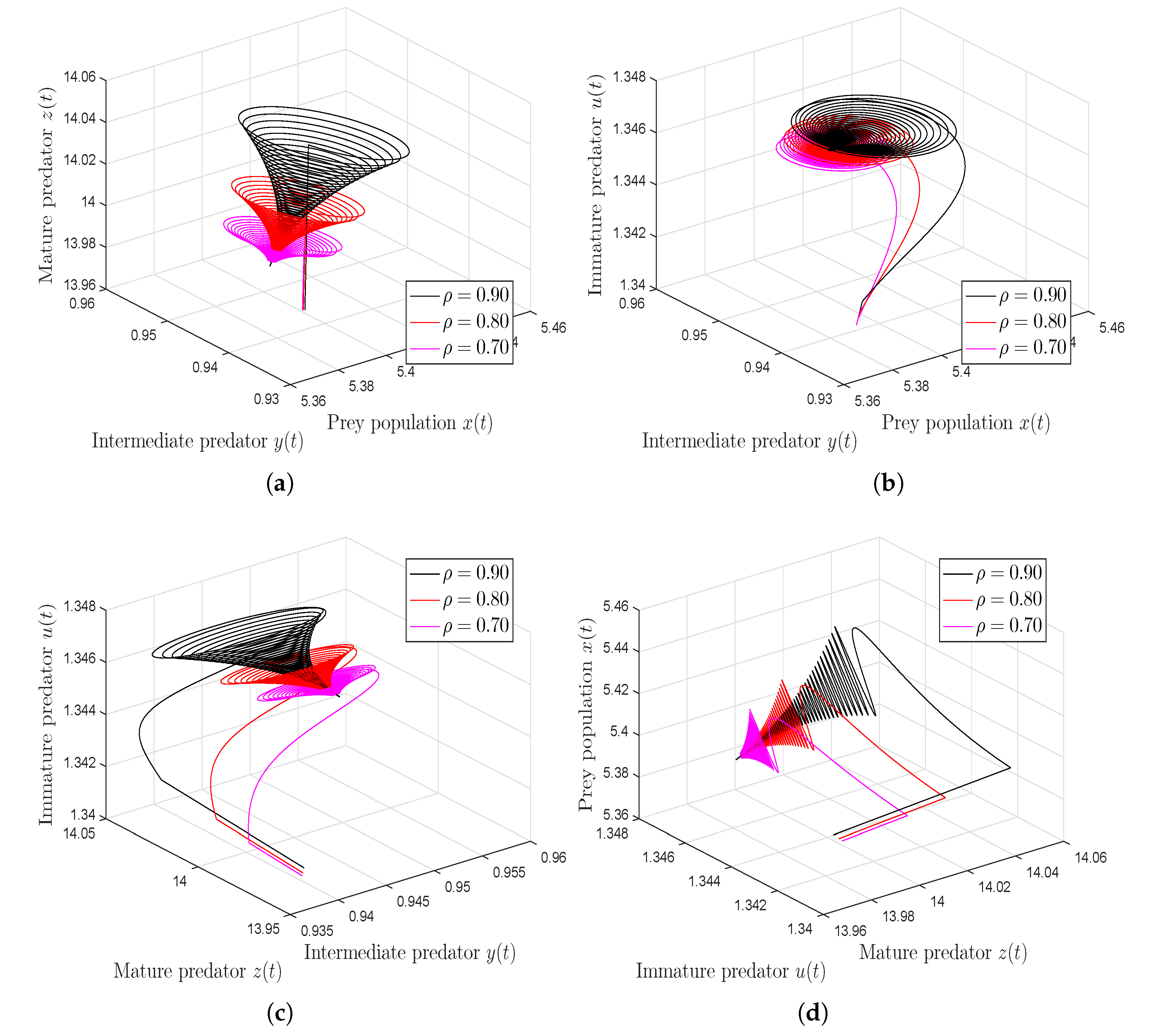
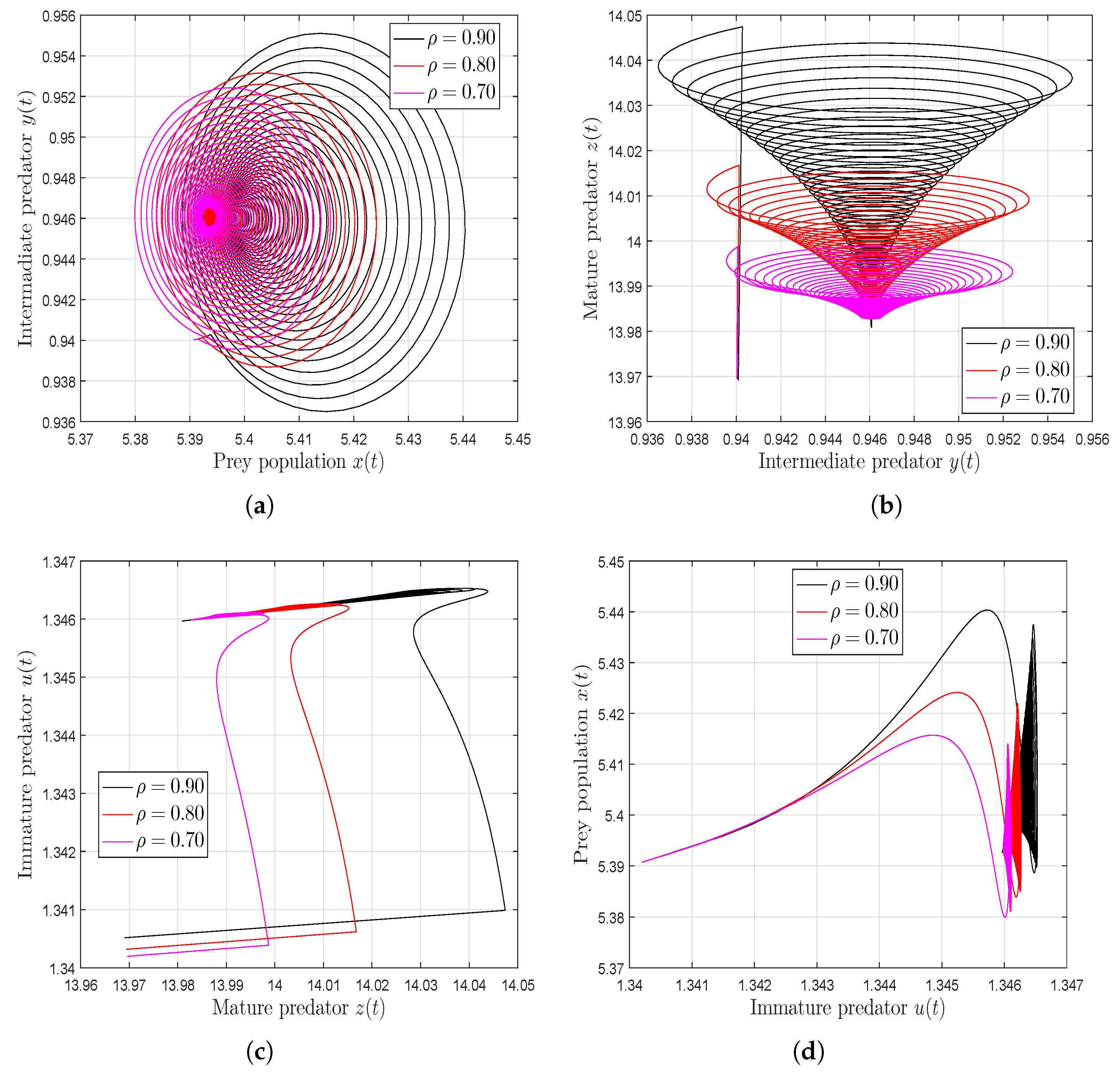
Generalized Caputo-type fractional derivatives also possess the same properties as Caputo-type derivatives. In order to solve the fractional IVP efficiently, consistently, and accurately, the predictor–corrector (PC) scheme is one of the best available. We solved the projected model using the modified PC scheme in the current study. According to the generalized Caputo algorithm, adaptive PC schemes use a nonuniform grid, which differs from the derivative Caputo PC algorithm. In fractional calculus applications, the generalized fractional integral operator is a valuable tool for controlling and building mathematical models due to the effect of its parameters $\phi$ and $\rho$. This new generalized Caputo fractional derivative has extra features over the other fractional derivatives such as Caputo, Caputo–Fabrizio, and Atangana–Baleanu. There is another parameter $\rho$ that is very helpful to graphical simulations when it comes to true data, in addition to the fractional-order parameter $\phi$. Changing the parameter value $\rho$ allows us to see more kinds of graphs.

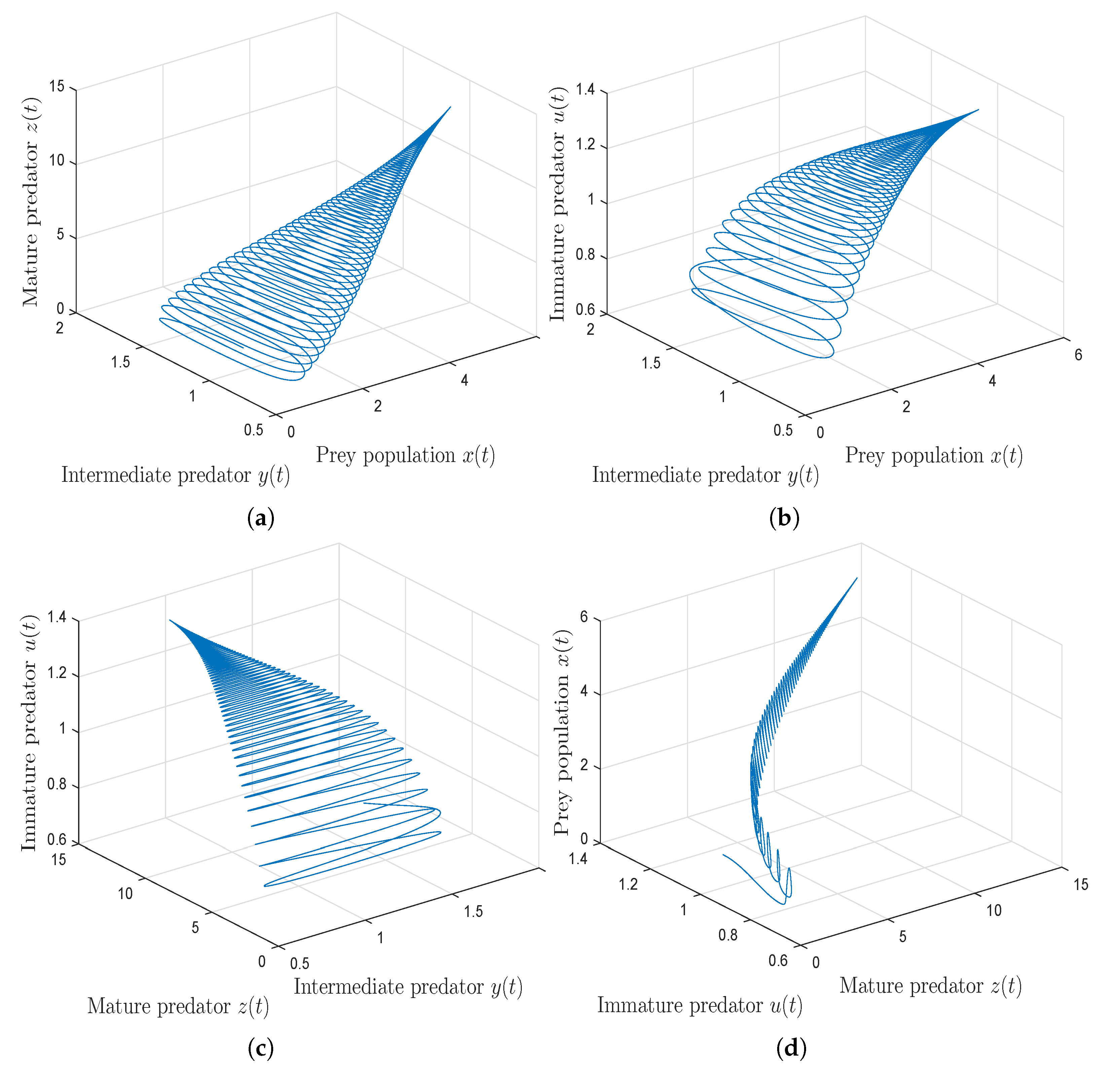
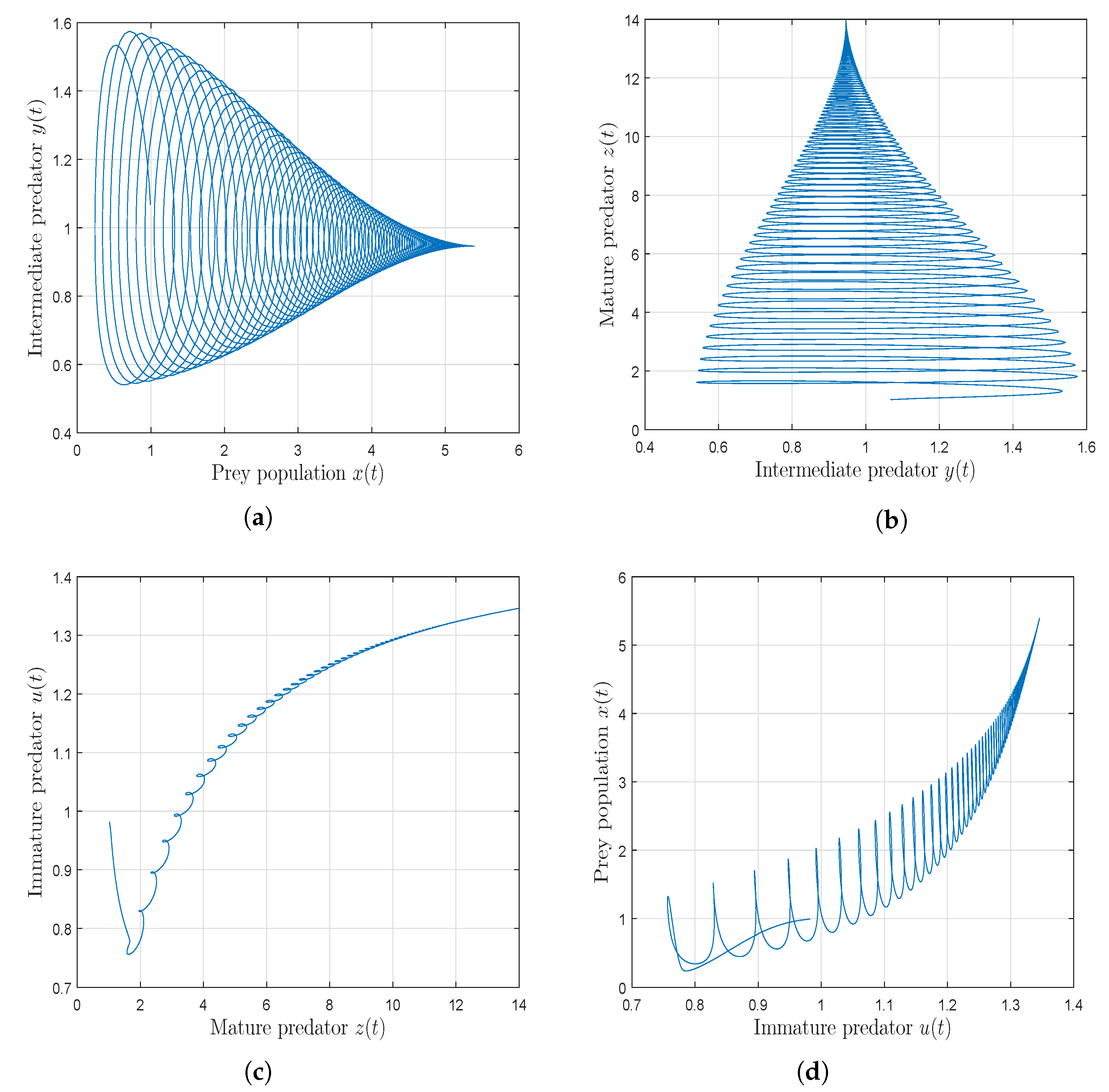
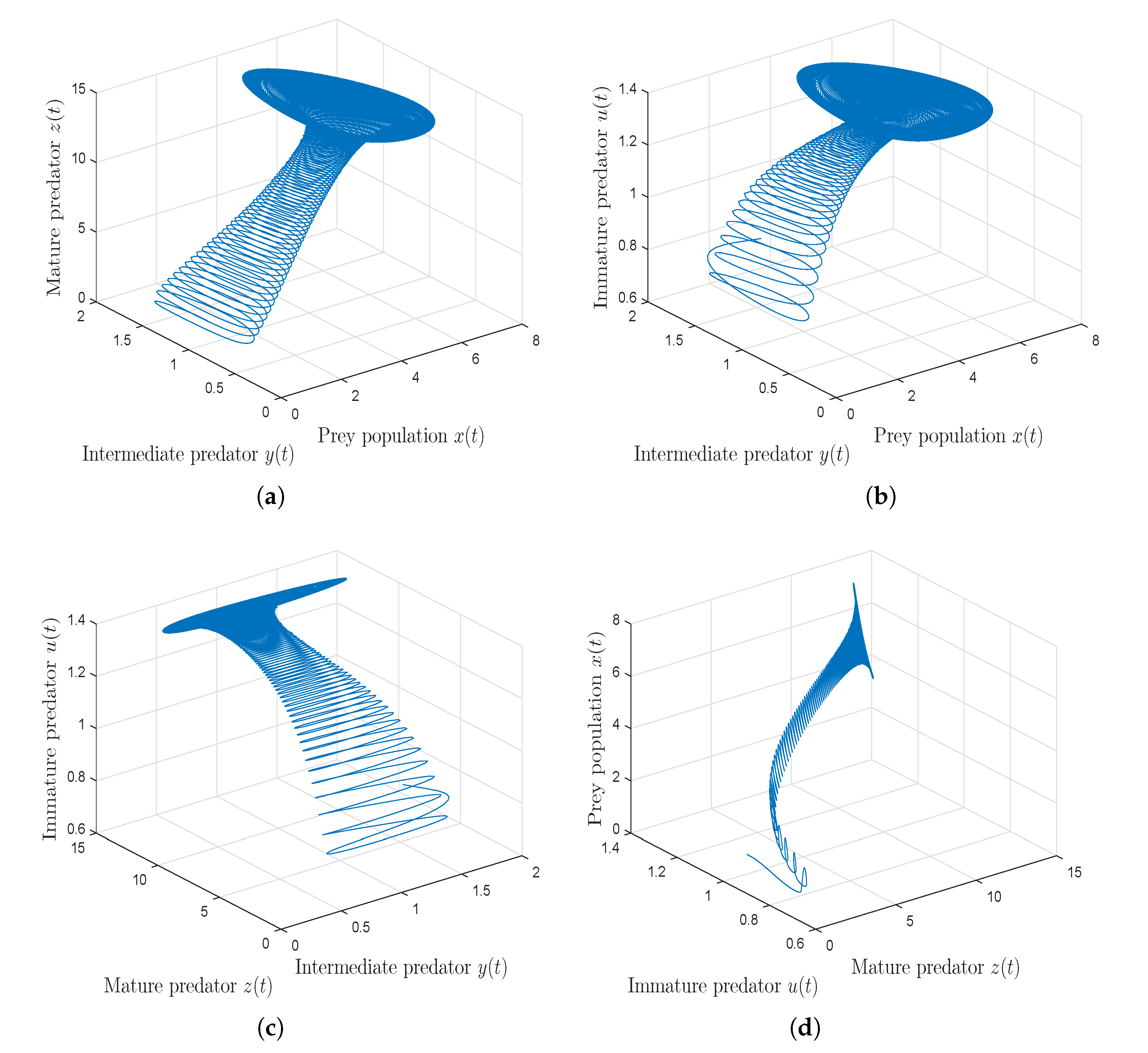
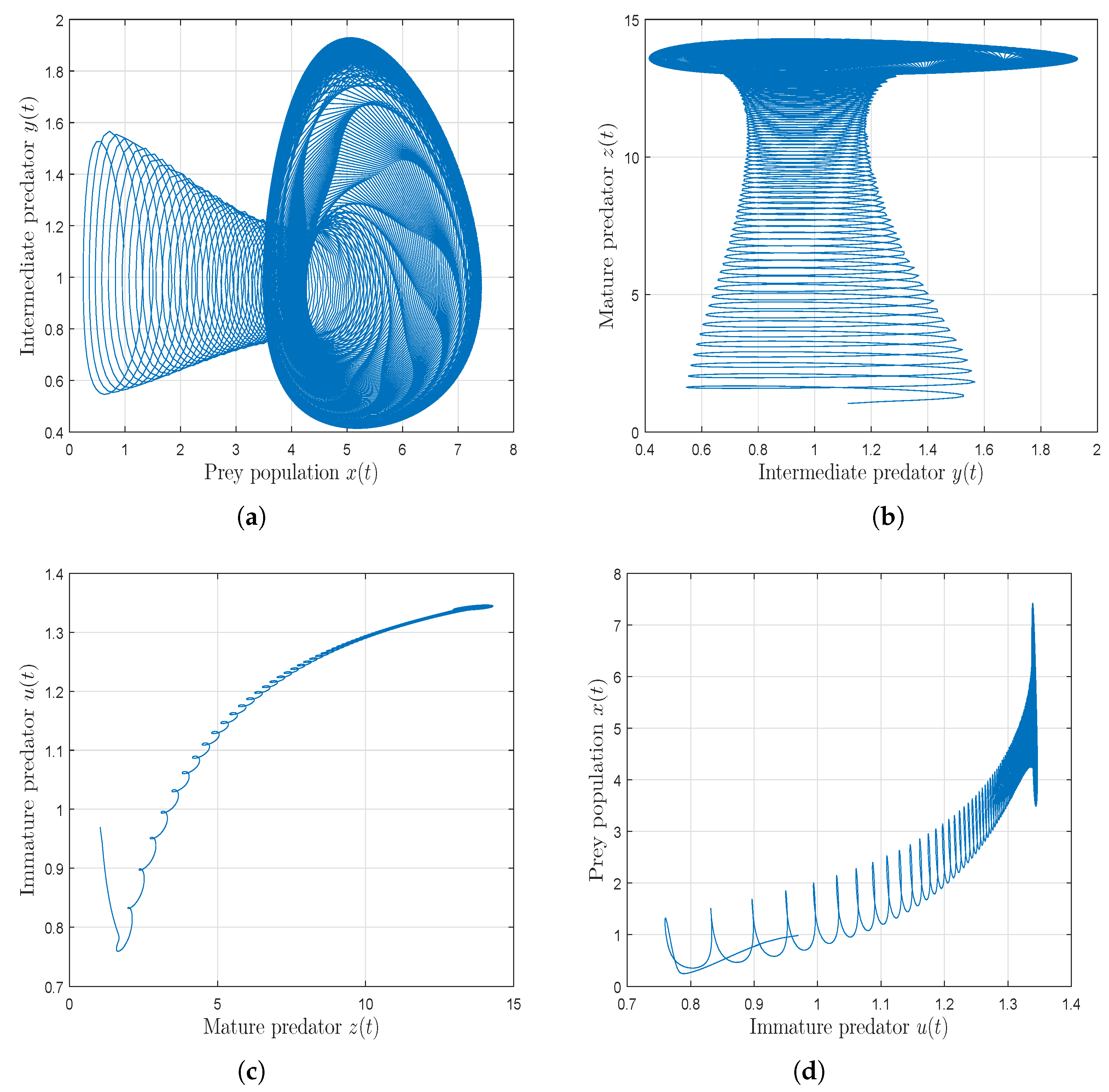
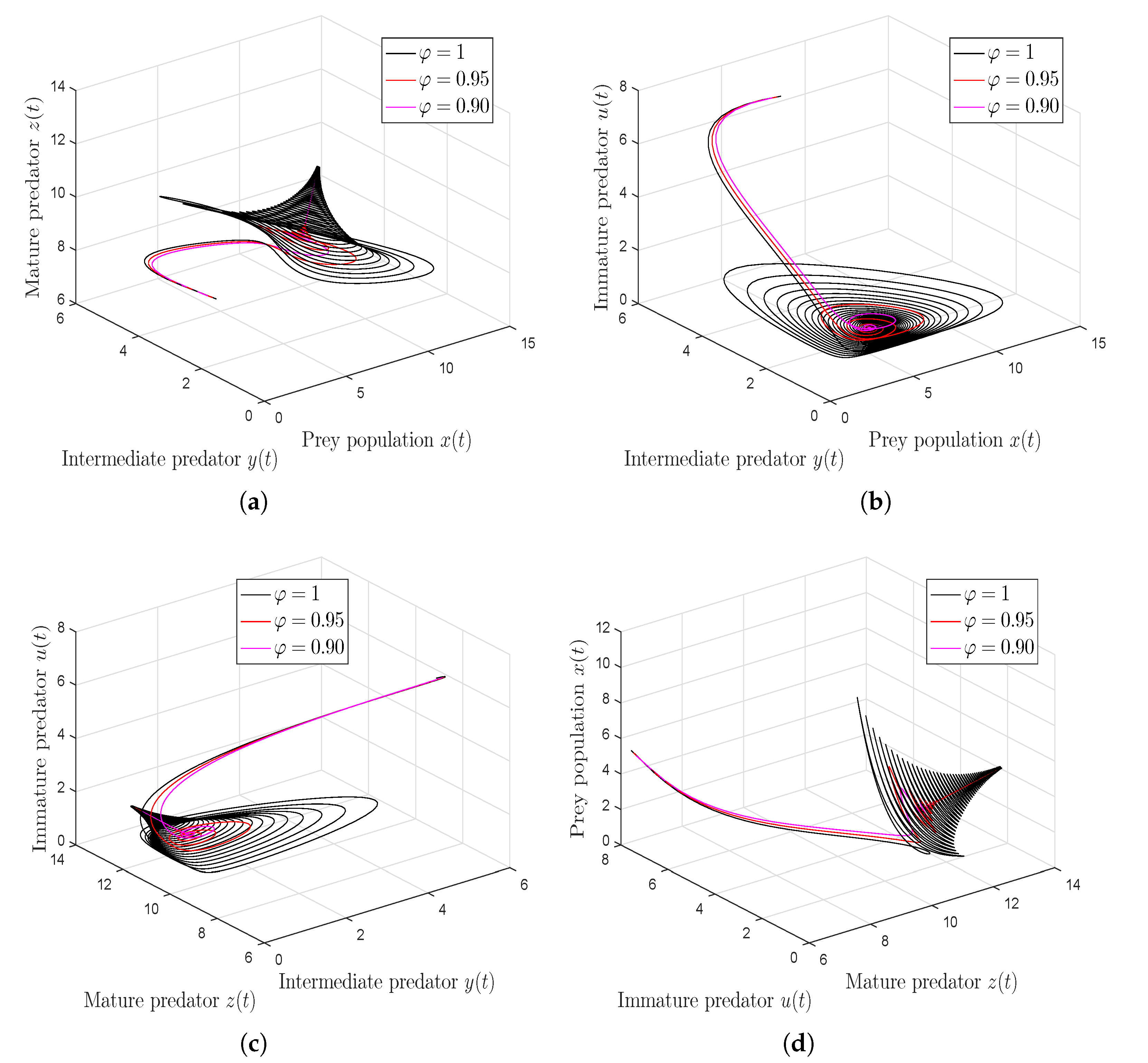
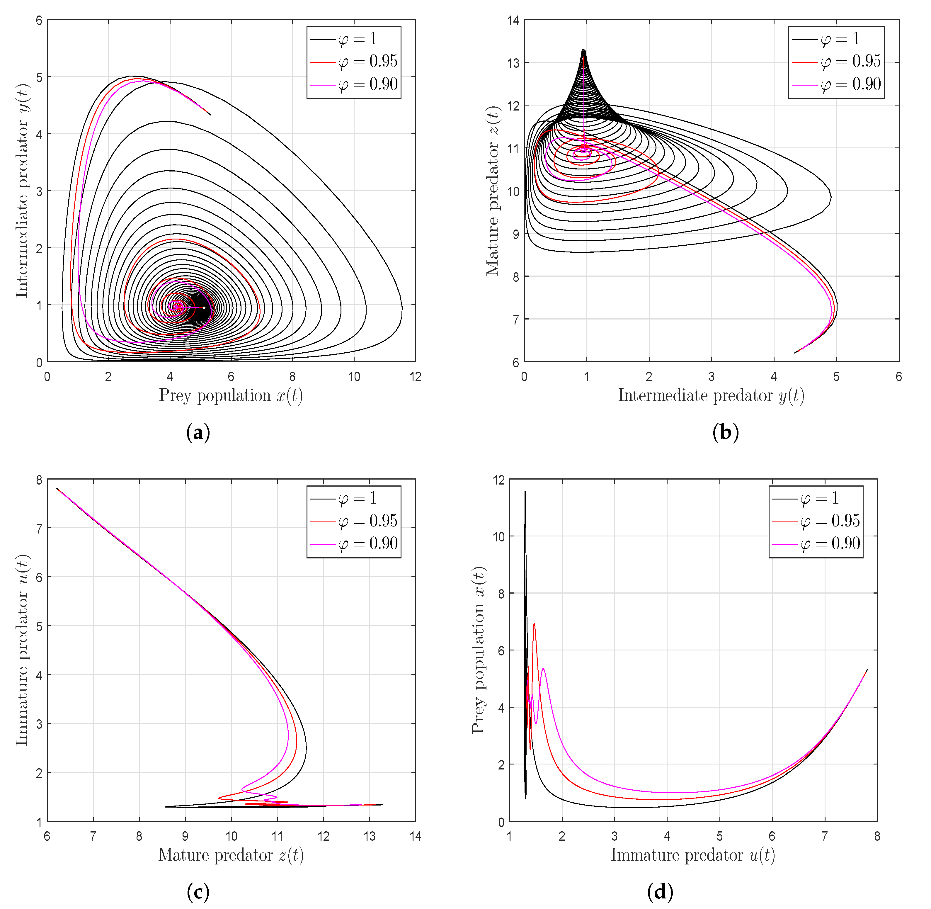
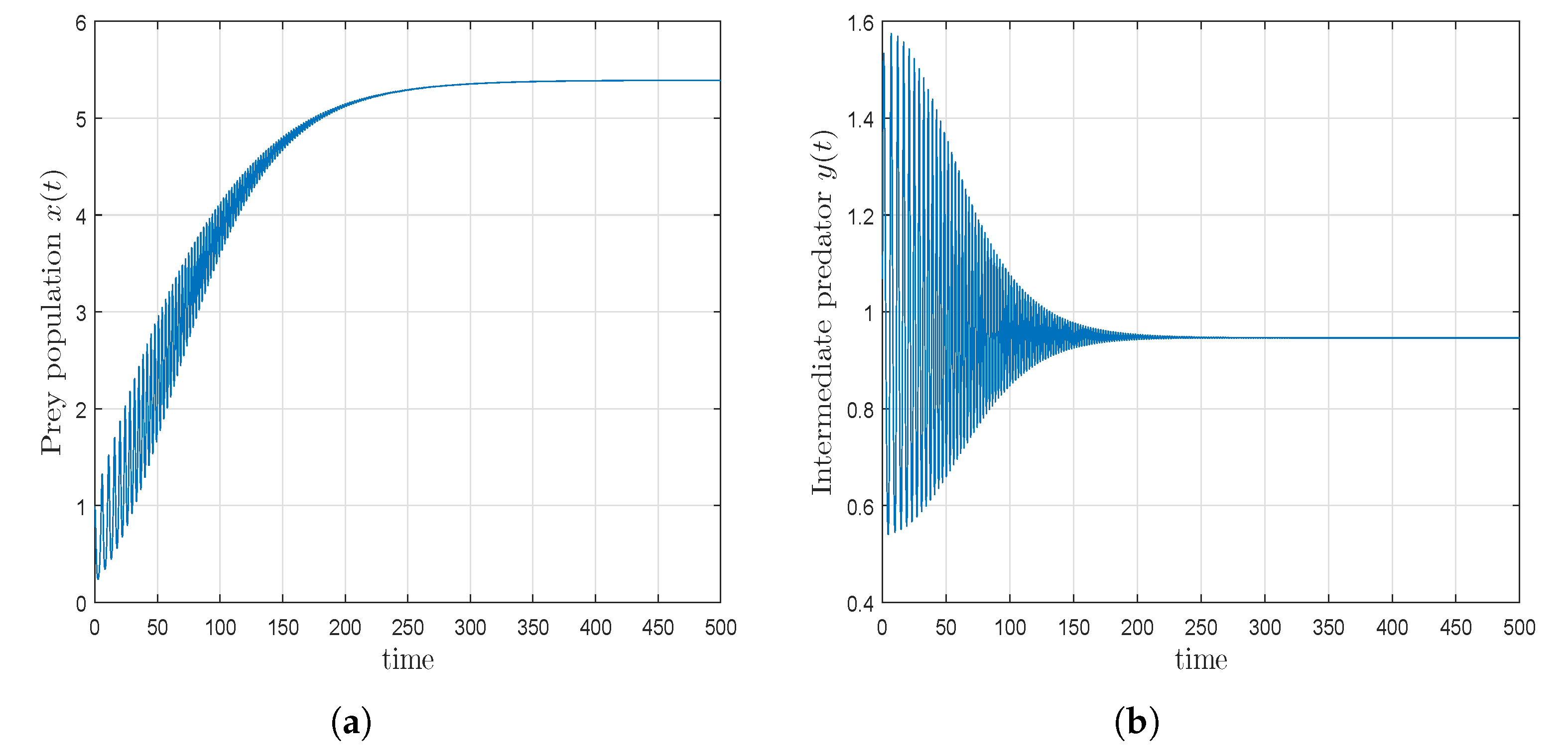
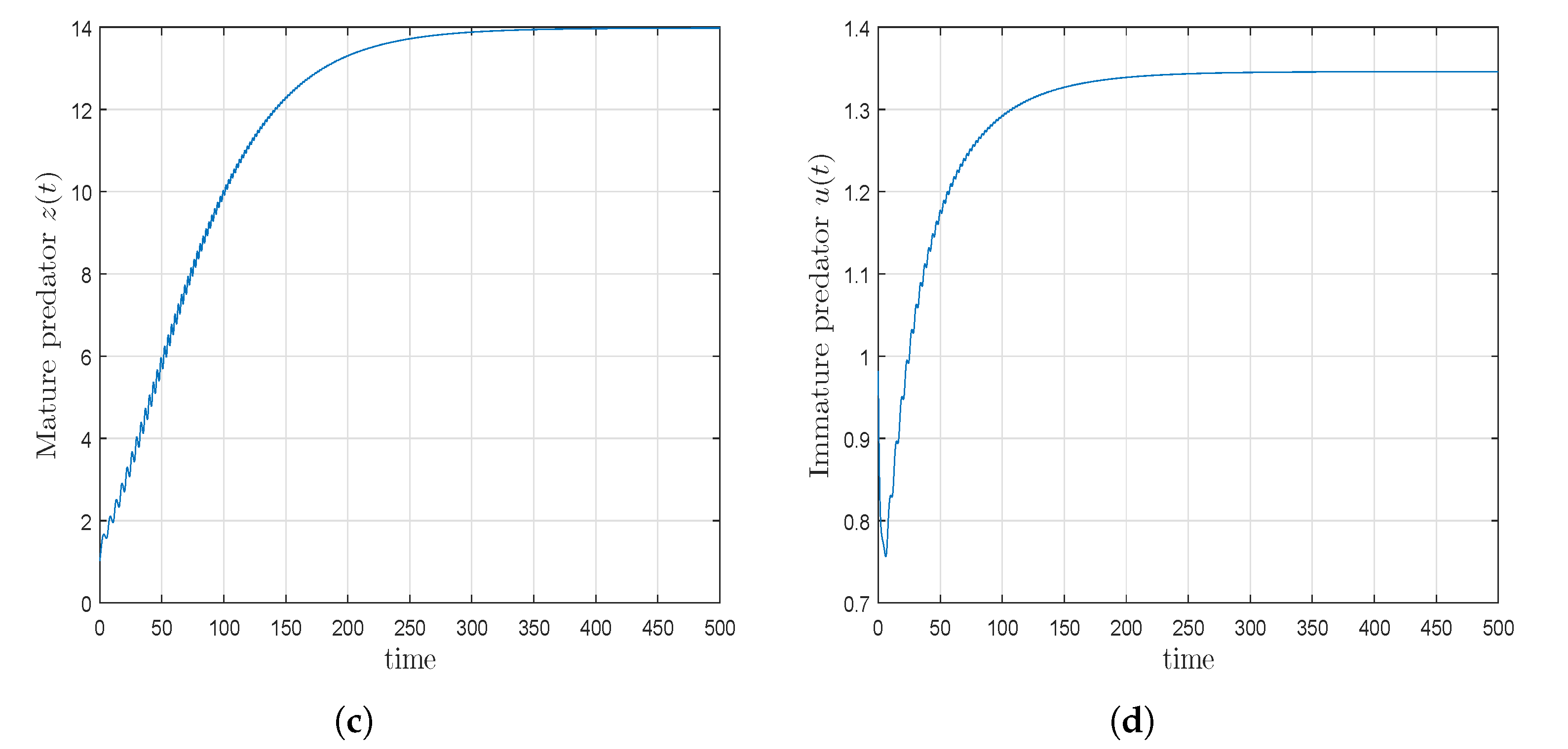
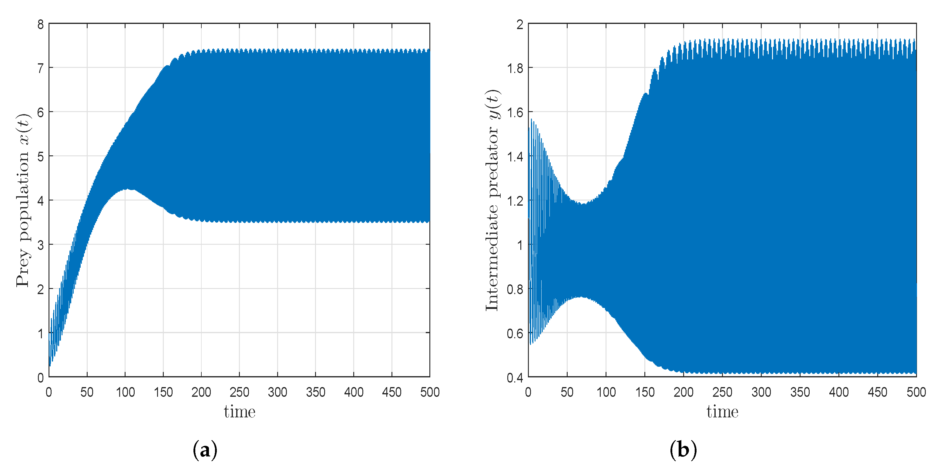
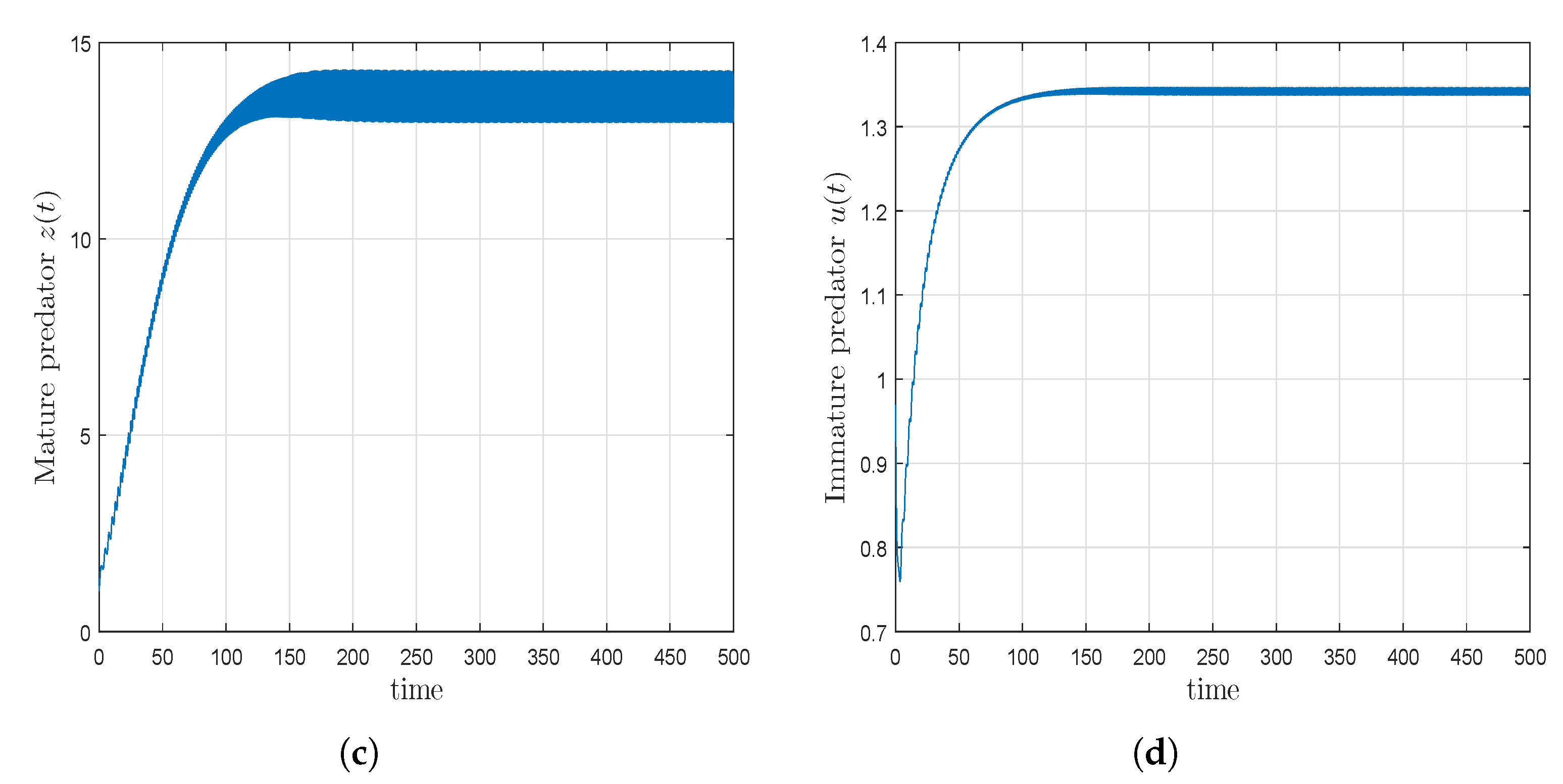
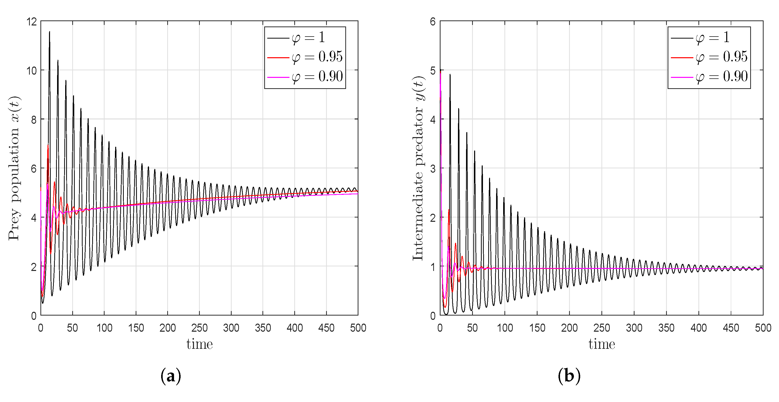
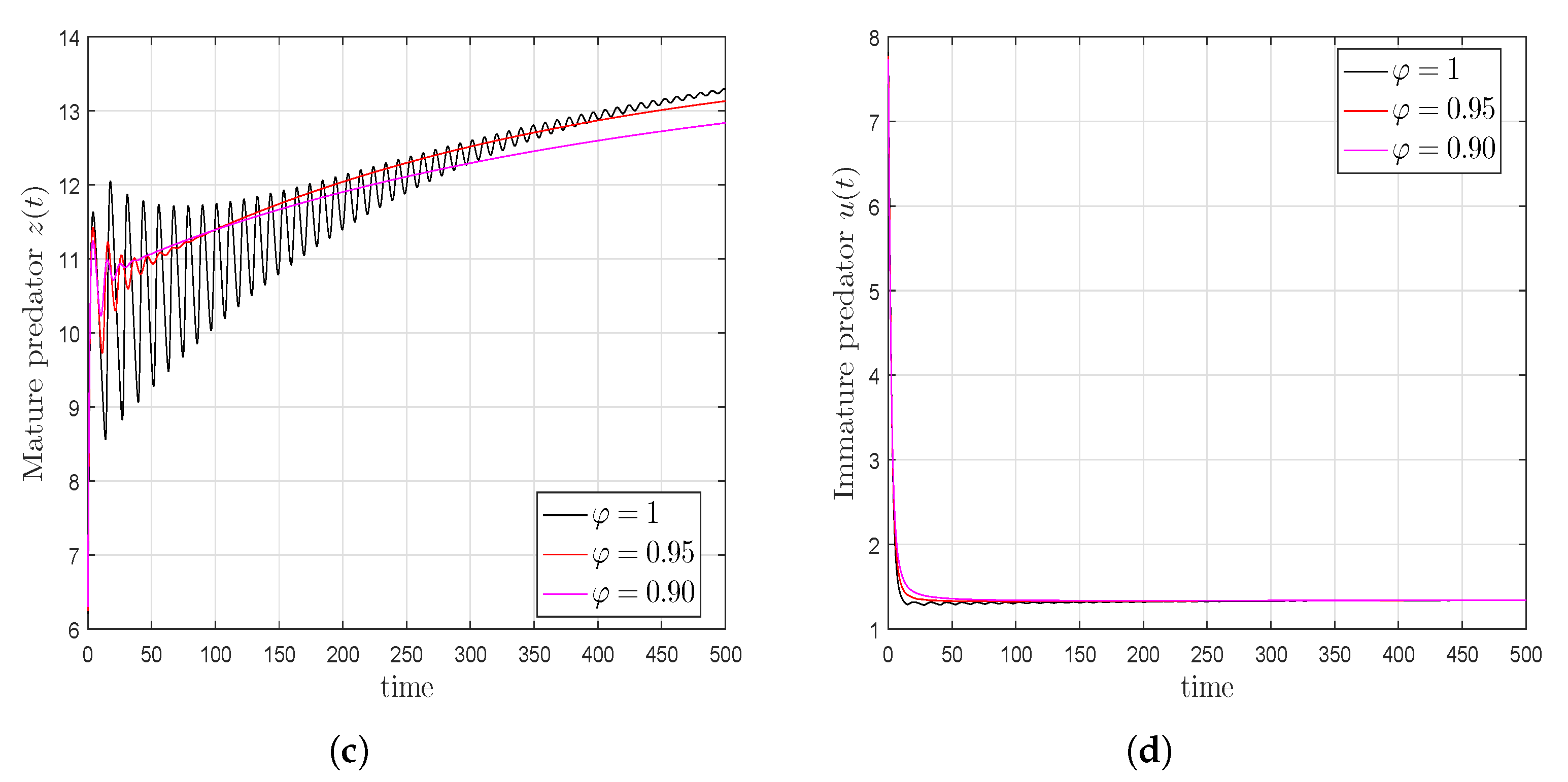
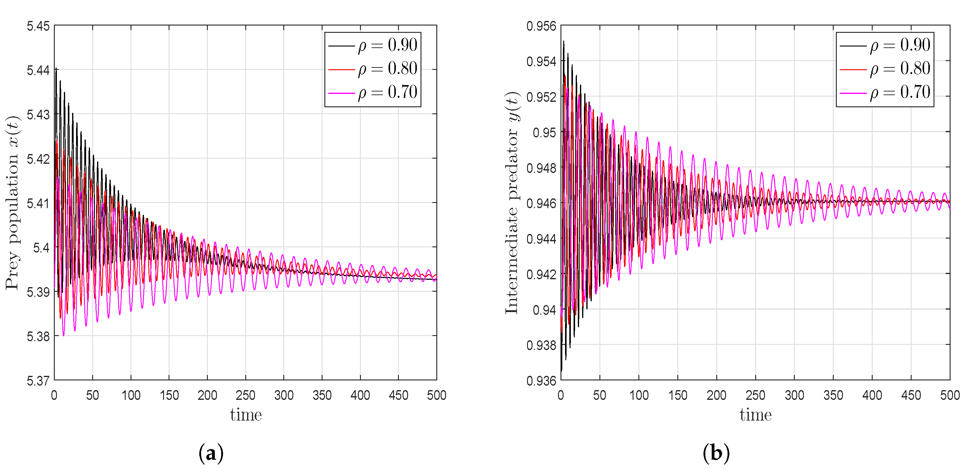
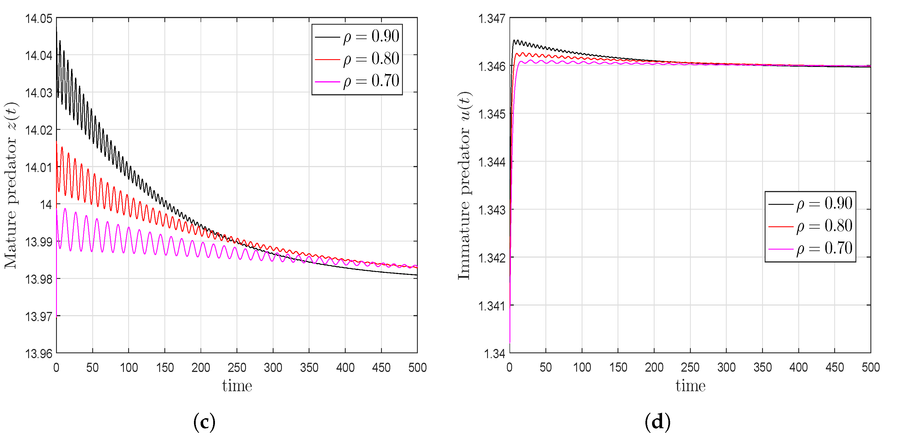
Figure 1 and Figure 2 illustrate the three-dimensional and two-dimensional dynamic phase portrait of the fractional food web system with the generalized Caputo derivative, respectively, when $\phi =1$ and $\rho =1.1$. Figure 3 exhibits the state variables x(t), y(t) z(t), and u(t) of the proposed model when $\phi =1$ and $\rho =1.1$. It can be seen that the value of $\rho$ strongly influences the characteristics of the fractional derivative, and this provides a different way of approaching control applications. Figure 4 and Figure 5 illustrate the three-dimensional and two-dimensional dynamic phase portrait of the fractional food web system with the generalized Caputo derivative, respectively, when $\phi =1$ and $\rho =1.1$. Figure 6 exhibits the state variables x(t), y(t) z(t), and u(t) of the proposed model when $\phi =1$ and $\rho =1.2$. At fixed $\rho$, depending on the fractional-order value, our fractional food web system displays the complexity of the chaotic phase portrait. Hence, Figure 7, Figure 8, Figure 9 are the graphical illustrations of the proposed system at different fractional-order $\phi =1,0.95,0.90$ and fixed $\rho$. Further, we took the different values of $\rho$ and $\phi$ to be fixed, then the fractional food web system exhibits different phase portraits, which are shown in Figure 10, Figure 11, Figure 12. During the simulation of models with two fractional parameters, we observed chaos, and we noticed that the dynamics became more complex.

8. Conclusions

Here, we examined a three-species food web model. According to this model, top predators are stage-structured, with a mature predator having a cannibalism trait. In the absence of the predator, the prey grows logistically at the first level. Food consumption at different levels of the food web is described by Lotka–Volterra functional responses. The proposed mathematical model of the food web was examined using the generalized Caputo fractional derivative. Using a fixed-point hypothesis, this study presented an investigation of the existence and uniqueness of the fractional food web system. The algorithm described in this study is based on a numerical technique called ‘predictor–corrector’, which allows the approximate solution of the fractional food web model to be found. We demonstrated the stability of this numerical method. The fractional food web model was geometrically presented under the generalized Caputo operator for different choices of $\phi$ and $\rho$. The new dynamical behaviour and phase portrait were demonstrated for various fractional orders ($\phi$) and the value of $\rho$. This graphical illustration showed how the order of derivatives and the system parameters greatly affect the system. The new generalized fractional derivative will be used in future efforts to model other biological systems with memory or with hereditary properties, as well as to identify other important properties of this new generalized derivative.

References

- Naji, R.K. Global stability and persistence of three species food web involving omnivory. Iraqi J. Sci. 2012, 53, 866–876. [Google Scholar]
- McCann, K.; Hastings, A. Re–evaluating the omnivory–stability relationship in food webs. Proc. R. Soc. Lond. Ser. B Biol. Sci. 1997, 264, 1249–1254. [Google Scholar] [CrossRef] [Green Version]
- Nath, B.; Das, K.P. Density dependent mortality of intermediate predator controls chaos-conclusion drawn from a tri-trophic food chain. J. Korean Soc. Ind. Appl. Math. 2018, 22, 179–199. [Google Scholar]
- Gakkhar, S.; Priyadarshi, A.; Banerjee, S. Complex behaviour in four species food-web model. J. Biol. Dyn. 2012, 6, 440–456. [Google Scholar] [CrossRef] [Green Version]
- Kondoh, M.; Kato, S.; Sakato, Y. Food webs are built up with nested subwebs. Ecology 2010, 91, 3123–3130. [Google Scholar] [CrossRef]
- Holt, R.D.; Grover, J.; Tilman, D. Simple rules for interspecific dominance in systems with exploitative and apparent competition. Am. Nat. 1994, 144, 741–771. [Google Scholar] [CrossRef]
- Huang, C.; Qiao, Y.; Huang, L.; Agarwal, R.P. Dynamical behaviours of a food-chain model with stage structure and time delays. Adv. Differ. Equ. 2018, 186. [Google Scholar] [CrossRef] [Green Version]
- Naji, R.K.; Ridha, H.F. The dynamics of four species food web model with stage structure. Int. J. Technol. Enhanc. Emerg. Eng. Res. 2016, 4, 13–32. [Google Scholar]
- Persson, L.; Roos, A.M.D.; Claessen, D.; Byström, P.; Lövgren, J.; Sjögren, S.; Svanbäck, R.; Wahlström, E.; Westman, E. Gigantic cannibals driving a whole-lake trophic cascade. Proc. Natl. Acad. Sci. USA 2003, 100, 4035–4039. [Google Scholar] [CrossRef] [Green Version]
- Van den Bosch, F.; Gabriel, W. Cannibalism in an age-structured predator-prey system. Bull. Math. Biol. 1997, 59, 551–567. [Google Scholar] [CrossRef]
- Jurado-Molina, J.; Gatica, C.; Cubillos, L.A. Incorporating cannibalism into an age-structured model for the chilean hake. Fish. Res. 2006, 82, 30–40. [Google Scholar] [CrossRef]
- Kohlmeier, C.; Ebenhöh, W. The stabilizing role of cannibalism in a predator-prey system. Bull. Math. Biol. 1995, 57, 401–411. [Google Scholar] [CrossRef]
- Diekmann, O.; Nisbet, R.; Gurney, W.; Van den Bosch, F. Simple mathematical models for cannibalism: A critique and a new approach. Math. Biosci. 1986, 78, 21–46. [Google Scholar] [CrossRef] [Green Version]
- Bhattacharyya, J.; Pal, S. Coexistence of competing predators in a coral reef ecosystem. Nonlinear Anal. Real World Appl. 2011, 12, 965–978. [Google Scholar] [CrossRef]
- Kumar, S.; Kumar, A.; Samet, B.; Dutta, H. A study on fractional host–parasitoid population dynamical model to describe insect species. Numer. Methods Partial. Differ. Equ. 2021, 37, 1673–1692. [Google Scholar] [CrossRef]
- Kumar, S.; Kumar, A.; Jleli, M. A numerical analysis for fractional model of the spread of pests in tea plants. Numer. Methods Partial. Differ. Equ. 2022, 38, 540–565. [Google Scholar] [CrossRef]
- Kumar, S.; Kumar, A.; Samet, B.; Gómez-Aguilar, J.; Osman, M. A chaos study of tumor and effector cells in fractional tumor-immune model for cancer treatment. Chaos Solitons Fractals 2020, 141, 110321. [Google Scholar] [CrossRef]
- Kumar, A.; Kumar, S. A study on eco-epidemiological model with fractional operators. Chaos Solitons Fractals 2022, 156, 111697. [Google Scholar] [CrossRef]
- Kumar, A.; Alshahrani, B.; Yakout, H.; Abdel-Aty, A.-H.; Kumar, S. Dynamical study on three-species population eco-epidemiological model with fractional order derivatives. Results Phys. 2021, 24, 104074. [Google Scholar] [CrossRef]
- Kumar, S.; Kumar, A.; Abdel-Aty, A.-H.; Alharthi, M. A study on four-species fractional population competition dynamical model. Results Phys. 2021, 24, 104089. [Google Scholar] [CrossRef]
- Kilbas, A.A.; Srivastava, H.M.; Trujillo, J.J. Theory and Applications of Fractional Differential Equations; Elsevier: Amsterdam, The Netherlands, 2006. [Google Scholar]
- Atangana, A.; Baleanu, D. New fractional derivatives with nonlocal and non-singular kernel: Theory and application to heat transfer model. arXiv 2016, arXiv:1602.03408. [Google Scholar] [CrossRef] [Green Version]
- Caputo, M.; Fabrizio, M. A new definition of fractional derivative without singular kernel. Prog. Fract. Differ. Appl. 2015, 1, 1–13. [Google Scholar]
- Khan, A.; Abdeljawad, T.; Gomez-Aguilar, J.; Khan, H. Dynamical study of fractional order mutualism parasitism food web module. Chaos Solitons Fractals 2020, 134, 109685. [Google Scholar] [CrossRef]
- Katugampola, U.N. New approach to a generalized fractional integral. Appl. Math. Comput. 2011, 218, 860–865. [Google Scholar] [CrossRef] [Green Version]
- Katugampola, U.N. A new approach to generalized fractional derivatives. arXiv 2011, arXiv:1106.0965. [Google Scholar]
- Odibat, Z.; Baleanu, D. Numerical simulation of initial value problems with generalized Caputo-type fractional derivatives. Appl. Numer. Math. 2020, 156, 94–105. [Google Scholar] [CrossRef]
- Alqahtani, R.T.; Ahmad, S.; Akgül, A. Dynamical analysis of bio-ethanol production model under generalized nonlocal operator in Caputo sense. Mathematics 2021, 9, 2370. [Google Scholar] [CrossRef]
- Erturk, V.S.; Kumar, P. Solution of a COVID-19 model via new generalized Caputo-type fractional derivatives. Chaos Solitons Fractals 2020, 139, 110280. [Google Scholar] [CrossRef]
- Liu, Y.; Roberts, J.; Yan, Y. A note on finite difference methods for nonlinear fractional differential equations with non-uniform meshes. Int. J. Comput. Math. 2018, 95, 1151–1169. [Google Scholar] [CrossRef]
- Dimitrov, Y. Approximations of the Fractional Integral and Numerical Solutions of Fractional Integral Equations. Commun. Appl. Math. Comput. 2021, 3, 545–569. [Google Scholar] [CrossRef]
- Diethelm, K.; Ford, N.J.; Freed, A.D. A predictor–corrector approach for the numerical solution of fractional differential equations. Nonlinear Dyn. 2002, 29, 3–22. [Google Scholar] [CrossRef]
- Kumar, P.; Erturk, V.S.; Kumar, A. A new technique to solve generalized Caputo type fractional differential equations with the example of computer virus model. J. Math. Ext. 2021, 15, 1–23. [Google Scholar] [CrossRef]
- Ibrahim, H.A.; Naji, R.K. The complex dynamic in three species food webmodel involving stage structure and cannibalism. AIP Conf. Proc. 2020, 2292, 020006. [Google Scholar]