Fatigue Life Assessment of Intercity Track Viaduct Based on Vehicle–Bridge Coupled System

Abstract

During the long-term operation of an urban railway viaduct, it is subjected to multiple cyclic loads caused by the movement of a vehicle. As a result, the fatigue life of the bridge should be fully considered during the design process. Furthermore, the bridge structure will be subject to environmental corrosion for an extended period of time, resulting in concrete carbonization and reinforcement corrosion, which aggravates the bridge structure’s fatigue damage. To compensate for the disadvantage of the traditional static analysis method’s inability to consider vehicle speed, a vehicle–bridge system coupled model is established, material corrosion is considered, railway bridge damage under vehicle load is analyzed, and the service life of common 30 m and 25 m span bridges is calculated. The results show that ignoring corrosion will understate the bridge damage, and vehicle speed has a significant impact on bridge fatigue life. Finally, the recommended operating speeds for 30 m span and 25 m span bridges are provided.

1. Introduction

The original highway transportation system was unable to meet the people’s travel needs due to the city’s rapid development. As a result, stable, fast, and special rail transit has become an important urban transportation infrastructure. The subway is currently the most important urban rail transit infrastructure. For various reasons, the subway cannot be built in some areas of the city, so a viaduct is used instead. The train will cause bridge vibration as it passes through the viaduct. Due to the high operation frequency and long operation time of urban rail transit, the fatigue resistance of the viaduct should be fully considered to ensure the line’s long-term operation safety.

At the moment, the most common type of rail transit viaduct is a reinforced concrete structure. Many academics have investigated the fatigue performance of rail bridge structures. Some scholars focused on the fatigue mechanical properties of the track bridge system, especially interlayer components, and have carried out a series of studies from the perspective of tests. For example, Sheng et al. [1] studied the fatigue performance of a unit-track slab in a long-span cable-stayed bridge through a full-scale fatigue performance test; Zhou et al. [2] and Zhao et al. [3] completed the experimental study on the mechanical properties of the CRTS II track slab bridge system under fatigue load and proposed the calculation formula of stiffness degradation of the system according to the test results. Zeng et al. [4] completed the research on the fatigue mechanical properties of a full-scale CRTS III track slab system under fatigue load. The results show that the stiffness of fasteners and interlayer components in the track system will change under cyclic load. The above researchers obtained the fatigue characteristics of track bridge system from the test results, and proposed some empirical formulas, which provided valuable data for follow-up research. Track plate structure is a multi-layer composite plate structure, and the connecting layer between plates will inevitably become a weak part [5].

Because the viaduct structure is exposed to the wind and rain for a long time, the carbonation of concrete and the corrosion of reinforcement is inevitable in the long-term operation. Many scholars believe that in considering the long-term operation, in addition to the mechanical properties, it is necessary to consider the impact of durability problems, such as carbonation and corrosion. In the work of Song et al. [6], the experimental study on the fatigue performance of small-span concrete bridge deck was completed, and on this basis, they considered the corrosion effect of the structure, and evaluated the service life of the bridge deck under the load of a heavy load train. Cui et al. [7] also considered the corrosion effect of the structure and analyzed the fatigue life of the bridge in different environments. In addition to the corrosion fatigue of track plate components, the corrosion fatigue of rail components is also an object that needs attention [8].

The vehicle–bridge coupled system analysis approach is commonly used in the dynamic response analysis of track and bridge structures under train load, as it can more correctly represent the bridge reaction under train load [9]. The coupled system analysis method, as opposed to the static method that considers the dynamic impact factor, can take into account the influence of vehicle speed and track irregularity [10,11,12,13]. Different from the component research, the system model usually needs to be studied by means of numerical calculation. For example, in the work of Li et al. [14], the reliability of the anti-fatigue performance of the steel structure bridge was evaluated based on the numerical model of the vehicle–bridge coupled system considering randomness. Wang et al. [15] evaluated the fatigue performance of a concrete bridge based on the vehicle–bridge coupled model and compared the calculation results with the moving load method and moving mass method. Xu et al. [16] established a vehicle track system coupled model to analyze the fatigue damage evolution of the track system under vehicle load, and the results showed that compared with only considering fatigue or interface damage, the effects of both should be considered comprehensively. Nowadays, machine learning has become a hot topic. Similarly, the fatigue performance of bridges can be analyzed by using the machine learning technology [17]. In addition, the fatigue analysis can also be analyzed in combination with field test and numerical technology, so as to ensure the reliability of the results; Li and Wu [18] proposed a framework for the fatigue evaluation of key details of steel bridge through multi-scale dynamic analysis of the train track bridge system and linear elastic fracture mechanics and studied the effects of track irregularity and train running speed on fatigue crack propagation life. Taking into consideration the vehicle speed and its irregularity is possible using SHM systems mounted on/in the bridges [19,20,21].

The findings of the above studies demonstrate that vehicle speed and environmental corrosion have a significant impact on fatigue life and long-term bridge damage. Although there are many studies at present, the consideration in the study of fatigue performance is still not comprehensive, such as only considering the dynamic performance and ignoring the influence of environmental factors on materials, or only studying the fatigue static mechanical performance of the track–bridge system. In order to more accurately predict the fatigue life of an urban rail viaduct so that engineering designers and researchers can refer to it, the vehicle–bridge system coupled model will be constructed, and the corrosion effect of the environment on the fatigue life of viaduct will be studied.

2. Vehicle–Bridge Coupled System

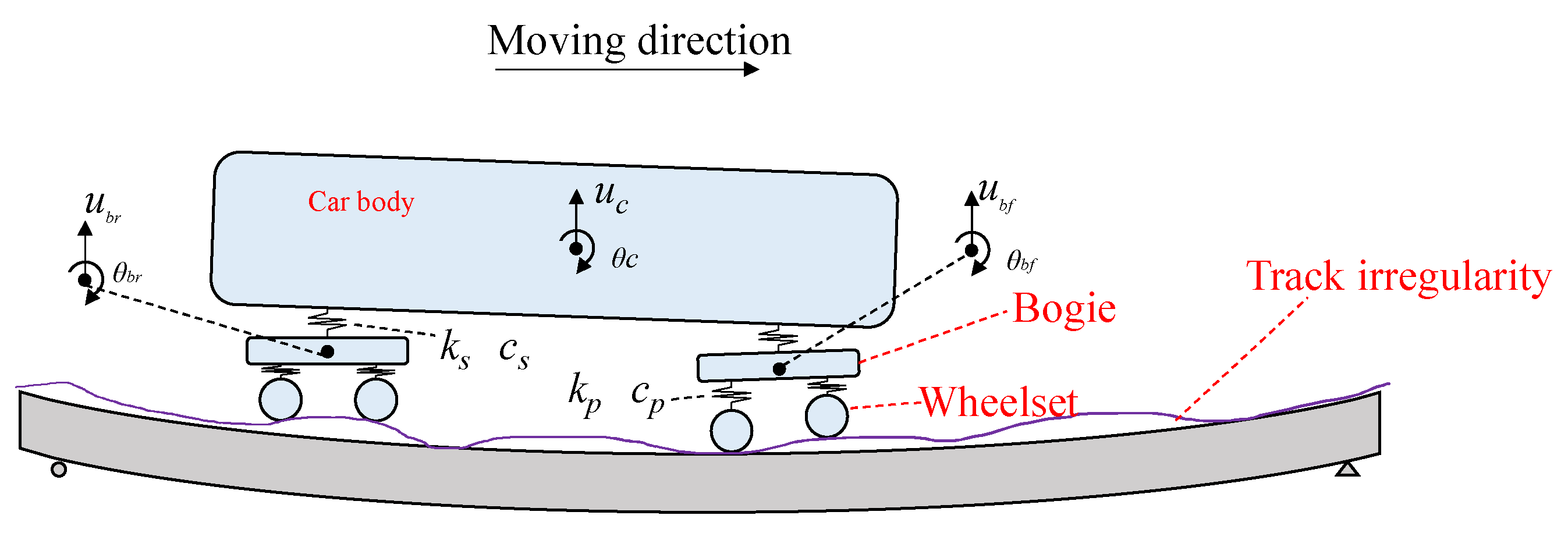
2.1. Vehicle Model

Multi-body dynamics is used to simulate the vehicle. Each vehicle is made up of one car body, two bogies, and four wheel sets, as shown in Figure 1. Secondary suspension refers to the suspension system between the car body and the bogie, while primary suspension refers to the suspension system between the bogie and the wheel set. The suspension systems are simulated using spring-viscous damping, where k_p and c_p represent the stiffness and damping of the primary suspension’s spring, respectively, and k_s and c_s represent the stiffness and damping of the secondary suspension’s spring, respectively.

Each car body has two degrees of freedom, including vertical u_c and rotating θ_c; the front bogie has two degrees of freedom, including vertical u_bf and rotation θ_bf; the rear bogie has two degrees of freedom, including vertical u_br and rotation θ_br; and each wheel set has one vertical degree of freedom, totaling ten degrees of freedom for the entire train. Because the coupled system’s wheel rail contact uses the close-fitting model, the wheel set is always in contact with the rail, and the wheel set has no independent degrees of freedom, the entire carriage has only six degrees of freedom.

2.2. Bridge Dynamics

The viaduct is modeled by the finite element method (FEM). Since the main research object is the girder, the influence of the pier is ignored in the model. The boundary condition of the bridge is the ideal hinge at the bearing position. The mass matrix M_b and stiffness matrix K_b of the bridge can be easily obtained. The damping matrix C_b adopts Rayleigh damping, and the damping ratio of each order is 2%. More details can also be found in Ref. [10].

2.3. Coupled System Dynamics

2.3.1. System Dynamic Formula

$$M_s{\ddot{X}}_s+C_s{\dot{X}}_s+K_s{X}_s=F_s$$

(1)

where $M_s$, $K_s$ and $C_s$ denote the coupled system’s mass matrix, stiffness matrix and damping matrix respectively; ${\ddot{X}}_s$, ${\dot{X}}_s$ and $X_s$ denote acceleration vector, velocity vector and displacement vector of coupled system, respectively; and $F_s$ denotes the force vector of the coupled system.

2.3.2. Mass Matrix

Mass matrix $M_s$ can be written as,

$$M_s=\left[\begin{array}{cc}{M}_v& \\ & M_b^{\prime }\end{array}\right]$$

(2)

where $M_v$ denotes the mass matrix of vehicle, and it can be written by the following formula,

$$M_v=\mathrm{diag}\left[\begin{array}{cccc}{M}_{v1}& M_{v2}& \dots & M_{vN}\end{array}\right]$$

(3)

where N represents the number of carriages; $M_{vi}$ denotes the i-th carriage mass matrix, and it can be written as,

$$M_{vi}=\mathrm{diag}\left[\begin{array}{cccccc}{m}_c& I_c& m_{bf}& I_{br}& m_{bf}& I_{br}\end{array}\right]$$

(4)

where m_c and I_c denote the mass and the moment of inertia of car body, respectively; m_bf and I_bf denote the mass and moment of inertia of the front bogie, respectively; and m_br and I_br denote the mass and moment of inertia of the rear bogie, respectively.

$M_b^{\prime }$ denotes the mass matrix of the bridge considering the wheelset coupling, and it can be written as,

$$M_b^{\prime }=M_b+{\displaystyle \sum }_h^N{\displaystyle \sum }_w^4{m}_w{N}_{hw}^T{N}_{hw}^{}$$

(5)

where m_w represents the mass of wheelset; N_hw represents the shape function corresponding to the position of the w-th wheelset in the h-th carriage. It is a time-varying array, and it can be written as,

$$N_{hw}=\left[\begin{array}{cccccccccc}0& \cdots & 0& N_h^1\left(x\right)& N_h^2\left(x\right)& N_h^3\left(x\right)& N_h^4\left(x\right)& 0& \cdots & 0\end{array}\right]$$

(6)

with

$$\{\begin{array}{l}{N}_h^1=1-3{\left(x/l^2\right)}^2+2{\left(x/l^2\right)}^3\hfill \\ N_h^2=\left(x/l\right)\left[1-2\left(x/l^2\right)+{\left(x/l^2\right)}^2\right]\hfill \\ N_h^3=3{\left(x/l^2\right)}^2-2{\left(x/l^2\right)}^3\hfill \\ N_h^4=\left(x/l\right)\left[{\left(x/l^2\right)}^2-\left(x/l^2\right)\right]\hfill \end{array}$$

(7)

where l denotes the length of element, and x denotes the distance between wheelset and left node of element.

2.3.3. Damping and Stiffness Matrices

The damping matrix of the coupled system can be written as,

$$C_s=\left[\begin{array}{cc}{C}_v& C_{vb}\\ C_{bv}& C_b^{\prime }\end{array}\right]$$

(8)

where $C_v$ represents the damping matrix of vehicle; $C_{vb}$ and $C_{bv}$ both represents the coupling damping matrix between vehicle and bridge. $C_b^{\prime }$ denotes the mass matrix of bridge considering the coupling of primary suspension.

$C_v$ can be expressed as,

$$C_v=\mathrm{diag}\left[\begin{array}{cccc}{C}_{v1}& C_{v2}& \dots & C_{vN}\end{array}\right]$$

(9)

$C_{vi}$ denotes the i-th carriage damping matrix, and it can be written as,

$$C_v=\left[\begin{array}{cccccc}2k_s& 0& -k_s& 0& -k_s& 0\\ & 2k_s{L}_2^2& -k_s{L}_2& 0& k_s{L}_2& 0\\ & & 2k_p+k_s& 0& 0& 0\\ & & & 2k_p{L}_1^2& 0& 0\\ & & & & 2k_p+k_s& 0\\ symm.& & & & & 2k_p{L}_1^2\end{array}\right]$$

(10)

where L₁ denotes the distance between two wheelsets, and L₂ denotes the distance between the two bogies.

$C_b^{\prime }$ can be expressed as,

$$C_b^{\prime }=C_b+{\displaystyle \sum }_h^N{\displaystyle \sum }_w^4{c}_p{N}_{hw}^T{N}_{hw}^{}$$

(11)

$C_{vb}$ and $C_{vb}$ can be expressed as,

$$C_{vb}=C_{vb}{}^T={\displaystyle \sum }_h^N{\displaystyle \sum }_w^4{C}_{vb,hw}$$

(12)

with

$$\{\begin{array}{c}{C}_{vb,h1}={\left[\begin{array}{cccccccc}0& 0& \cdots & -c_p{N}_{h1}& -c_p{L}_1{N}_{h1}& \cdots & 0& 0\end{array}\right]}^T\\ C_{vb,h2}={\left[\begin{array}{cccccccc}0& 0& \cdots & -c_p{N}_{h2}& -c_p{L}_1{N}_{h2}& \cdots & 0& 0\end{array}\right]}^T\\ C_{vb,h3}={\left[\begin{array}{cccccccc}0& 0& \cdots & -c_p{N}_{h1}& -c_p{L}_1{N}_{h1}& \cdots & 0& 0\end{array}\right]}^T\\ C_{vb,h4}={\left[\begin{array}{cccccccc}0& 0& \cdots & -c_p{N}_{h1}& -c_p{L}_1{N}_{h1}& \cdots & 0& 0\end{array}\right]}^T\end{array}$$

(13)

The stiffness matrix of the system can be obtained by replacing the letter c in Equations (8) to (13) with k.

2.3.4. Force Vector

The force vector of system $F_s$ can be expressed as,

$$F_s={\left[\begin{array}{cc}{F}_v& F_b\end{array}\right]}^T$$

(14)

with

$$F_v={\left[\begin{array}{cccc}{F}_{v1}& F_{v2}& \cdots & F_{vN}\end{array}\right]}^T$$

(15)

$$\begin{gathered} F_{vh}=c_p{\left[\begin{array}{cccccc}0& 0& {\dot{u}}_{r,h1}+{\dot{u}}_{r,h2}& L_1\left({\dot{u}}_{r,h1}-{\dot{u}}_{r,h2}\right)& {\dot{u}}_{r,h3}+{\dot{u}}_{r,h4}& L_1\left({\dot{u}}_{r,h3}-{\dot{u}}_{r,h4}\right)\end{array}\right]}^T \\ +k_p{\left[\begin{array}{cccccc}0& 0& u_{r,h1}+u_{r,h2}& L_1\left({\dot{u}}_{r,h1}-{\dot{u}}_{r,h2}\right)& u_{r,h3}+u_{r,h4}& L_1\left(u_{r,h3}-u_{r,h4}\right)\end{array}\right]}^T \end{gathered}$$

(16)

$$F_{\mathrm{b}}=-{\displaystyle \sum }_h^N{\displaystyle \sum }_w^4\left(m_w{\ddot{u}}_{r,hw}+c_p{\dot{u}}_{r,hw}+k_p{u}_{r,hw}+\left(0.25m_c+0.5m_t+m_w\right)g\right)N_{hw}{}^T$$

(17)

where $u_{r,hw}$ denotes the irregularity amplitude of w-th wheelset of h-carriage; ${\dot{u}}_{r,hw}$ and ${\ddot{u}}_{r,hw}$ denote the first derivative and the second derivative of $u_{r,hw}$, respectively.

2.4. Dynamic Stress Calculation

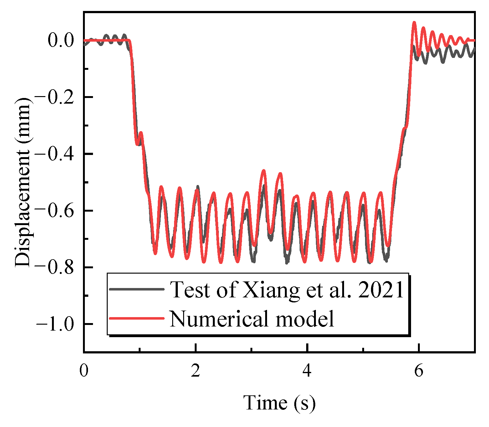
The stress dynamic response of the bridge is computed using the vehicle–bridge coupled system, and the fatigue performance of the structure or member is generally evaluated based on the stress under load. The displacement–strain relationship can be calculated using FEM theory, assuming that both ends of the element are solely subjected to the bending moment and shear force [14,15]; therefore, the relationship between strain and displacement is as follows,

$$\epsilon =B\delta$$

(18)

where $\epsilon$ denotes the strain of element; $\delta$ represents the displacement of the element node, and it can be expressed as,

$$\delta =\left[\begin{array}{cccc}{u}_i& {\theta }_i& u_j& {\theta }_j\end{array}\right]$$

(19)

where $u_i$ and ${\theta }_i$ denote the vertical and the rotation displacement of left node of element; $u_j$ and ${\theta }_j$ denote the vertical and the rotation displacement of right node of element. $B$ is the matrix of displacement–strain relationship, and it describes the transformation relationship between the strain at any point in the element and the displacement of the node in the element, and it is equal to the following formula,

$$B=-y\frac{d^{2}N}{d{x}^2}$$

(20)

where N is the shape function, and it is the same as Equation (7); y is the distance from the strain calculation point to the central axis (including sign). Further, B can be transformed into the following formula,

$$B=\left[\begin{array}{cccc}{\phi }_1& {\phi }_2& {\phi }_3& {\phi }_4\end{array}\right]$$

(21)

with

$$\{\begin{array}{l}{\phi }_1=\frac{6y}{l^2}\left(1-2\frac{x}{l}\right)\hfill \\ {\phi }_2=-\frac{2y}{l}\left(2-3\frac{x}{l}\right)\hfill \\ {\phi }_3=-\frac{6y}{l^2}\left(1-2\frac{x}{l}\right)\hfill \\ {\phi }_4=-\frac{2y}{l}\left(1-3\frac{x}{l}\right)\hfill \end{array}$$

(22)

After obtaining the strain, the stress can be calculated by the following formula,

$$\sigma =D\epsilon$$

(23)

where D is the stress–strain relationship matrix, and when assuming that the material stress–strain relationship D in the long-term operation of the bridge is linear elasticity, then D equal to the elastic modulus E of material.

2.5. Validation

In the work of Xiang et al. [22], the dynamic performance of a railway simply supported bridge was tested on site. In order to verify the accuracy of the numerical model in this paper, the field test results were compared with the numerical calculation results, as shown in Figure 2. It can be found that the peak value and trend calculated by the numerical model are close to the field test results, which shows the reliability of the numerical calculation results.

3. Fatigue Assessment Theory

3.1. Reinforcement Corrosion Considered Carbonation

Carbonation will lead to reinforcing bar depassivation. Then, reinforcement corrosion will occur in the presence of oxygen and water. When the reinforcing bar is corroded, the cross-sectional area of the reinforcing bar decreases, resulting in a decrease in the fatigue resistance of the reinforcement. With the accumulation of corrosion products, the corrosion-induced cracking of concrete cover occurs, which also accelerates the transport of aggressive agents and the reinforcing bar corrosion rate. The fatigue damage caused by repeated loading accelerates the process of concrete carbonation and reinforcing bar corrosion, and corrosion decreases the fatigue resistance of the reinforcing bar. The following formula can be used to determine when the reinforcement begins to rust [6],

$$t_{\mathrm{cr},\mathrm{c}}=d_{\mathrm{cr},\mathrm{c}}/i_{\mathrm{ini}}+t_{ini}$$

(24)

with

$$t_{ini}={\left(\frac{c-X_0}{K}\right)}^2$$

(25)

$$K=3K_1{K}_2{K}_3{T}^{0.25}R{H}^{1.5}\left(1-RH\right)\sqrt{C_{C{O}_2}/0.03}\left(\frac{58}{f_{cu}}-0.76\right)$$

(26)

$$X_0=\left(1.2-0.35K^{0.5}\right)D_k-\frac{6}{m_{ef}+1.6}\left(1.5+0.84K\right)$$

(27)

$$i_{\mathrm{ini}}=7.53K_{\mathrm{cl}}{m}_{\mathrm{ef}}\left(0.75+0.0125T\right){(RH-0.45)}^{2/3}{c}^{-0.675}{f}_{\mathrm{cu}}^{-1.8}$$

(28)

$$d_{\mathrm{cr},\mathrm{c}}=0.012c/d_0+0.00084f_{\mathrm{cu}}+0.018$$

(29)

where t_ini denotes the start time of reinforcement corrosion caused by concrete carbonization; c is the concrete cover thickness; K is the carbonation coefficient in the theoretical carbonation model proposed by Papadakis et al. [23], and K₁ denotes the location factor, and it equals to 1.4 for the component corner and 1.0 for other areas respectively; K₂ denotes the curing factor, and it equals to 1.2; K₃ denotes the stress factor, and it equals to 1.0 for compression and 1.1 for tension respectively [24]; RH denotes the environmental relative humidity; f_cu is the compression strength of cube concrete; C_co2 represents the CO₂ concentration around the concrete surface; X₀ is the carbonization residue; m_ef is the local environmental coefficient; D_k is the coefficient related to c and carbonation coefficient K; i_ini is the corrosion rate of reinforcement before cracking of concrete cover, and K_cl is the correction factor of reinforcement position; d₀ is the initial diameter of reinforcement; the details can be found in Ref. [6].

Under the action of vehicle fatigue load, the concrete cover of the bridge will also crack, and the cracking time can be calculated by the following formula,

$$t_{\mathrm{cr}}={10}^{\frac{1.3681-f_{\mathrm{t},\mathrm{s}}^{max}/f_{\mathrm{t}}}{0.1214}}\cdot {{\displaystyle \sum }}^{ }{n}_{\mathrm{cr},i}$$

(30)

with

$$f_{\mathrm{t},\mathrm{s}}^{max}=\left(1.3681+0.1214\lg \frac{{{\displaystyle \sum }}^{ }{n}_{\mathrm{cr},i}\cdot {10}^{\frac{f_{\mathrm{t},i}^{max}/f_{\mathrm{t}}-1.3681}{0.1214}}}{{{\displaystyle \sum }}^{ }{n}_{\mathrm{cr},i}}\right)f_t$$

(31)

where f_t is the tension strength of concrete; ${{\displaystyle \sum }}^{ }{n}_{\mathrm{cr},i}$ is the total maximum tensile stress cycles of tensile concrete; $f_{\mathrm{t},i}^{max}$ is the i-th maximum tensile stress under vehicle load.

Therefore, the first time of rust expansion cracking (calculated by Equations (24)–(29)) and fatigue cracking (calculated by Equations (30) and (31)) is the cracking time, and it can be expressed as,

$$t_{\mathrm{cr}}=\min \left\{t_{\mathrm{cr},\mathrm{c}}, t_{\mathrm{cr},\mathrm{f}}\right\}$$

(32)

When the concrete cover is cracked, the internal reinforcement loses its protection and will be in direct contact with the external environment, resulting in the increase in the reinforcement corrosion rate. The corrosion rate i_cr after cracking can be estimated by the following formula,

$$i_{\mathrm{cr}}=\left(4.5-340i_{\mathrm{ini}}\right)i_{\mathrm{ini}}$$

(33)

If the fatigue cracking of the concrete cover occurs before the rust expansion cracking, the corrosion depth d_cr,f of the reinforcement can be calculated by the following formula,

$$d_{cr,f}=\{\begin{array}{ll}0,& t_{\mathrm{cr},\mathrm{f}}⩽t_{\mathrm{ini}}\\ i_{\mathrm{ini}}\left(t_{\mathrm{cr},\mathrm{f}}-t_{\mathrm{ini}}\right),& t_{\mathrm{cr},\mathrm{f}}>t_{\mathrm{ir}}\end{array}$$

(34)

Then the corrosion depth d_cr of reinforcement when concrete cracks can be calculated by the following formula,

$$d_{\mathrm{cr}}=\min \left\{d_{\mathrm{cr},\mathrm{c}},d_{\mathrm{cr},\mathrm{f}}\right\}$$

(35)

According to the above calculation model, the corrosion depth $d\left(t\right)$ of reinforcement can be expressed as

$$d\left(t\right)=\{\begin{array}{ll}0,\hfill & T<t_{\mathrm{ini}}\hfill \\ i_{\mathrm{ini}}\left(T-t_{\mathrm{ini}}\right),\hfill & t_{\mathrm{ini}}<T⩽t_{\mathrm{cr}}\hfill \\ d_{\mathrm{cr}}+i_{\mathrm{cr}}\left(T-t_{\mathrm{ini}}-t_{\mathrm{cr}}\right),\hfill & T>t_{\mathrm{cr}}\hfill \end{array}$$

(36)

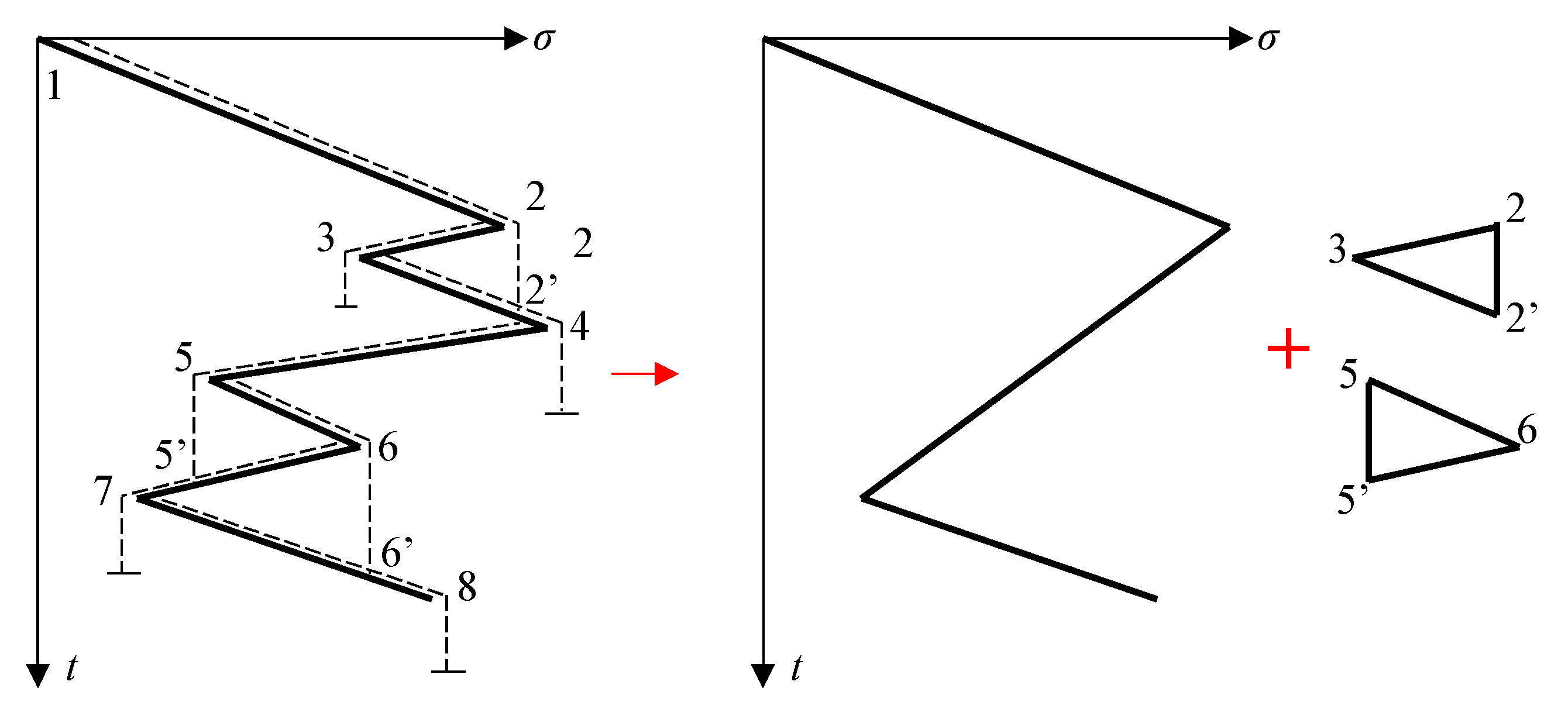
3.2. Fatigue Assessment Method

According to the S-N curve of reinforcement without considering corrosion, i.e.,

$$\lg N=\lg C-m\lg \mathsf{\Delta }\sigma$$

(37)

where C and m are both coefficient of steel reinforcement; $\mathsf{\Delta }\sigma$ is the stress range of steel reinforcement; and N is the number of stress cycles.

When the corrosion of material is considered, the coefficient of reinforcement C is a time-variable parameter, and it can be written as,

$$C\left(t\right)=C_0\varphi \left(t\right)$$

(38)

where $\varphi \left(t\right)$ is a time-varying coefficient fitted by experience, and it can be calculated by the following formula [25]

$$\varphi \left(t\right)=\{\begin{array}{ll}1,\hfill & d\left(t\right)<1.34 \mathrm{mm}\hfill \\ -0.79d{(t)}^2+1.88d\left(t\right)-0.1,\hfill & 1.34 \mathrm{mm}⩽d\left(t\right)⩽2.33 \mathrm{mm}\hfill \\ 0,\hfill & d\left(t\right)⩾2.33 \mathrm{mm}\hfill \end{array}\begin{array}{c}\\ \\ \end{array}$$

(39)

where C₀ denotes the coefficient of steel reinforcement without corrosion, and $d\left(t\right)$ is the corrosion depth, and it can be calculated from Equation (36).

Because the rusted part of the reinforcement can no longer withstand the original force, the non-rusted part must bear the entire original force, resulting in an increase in the reinforcement stress amplitude. The following is the time-varying model of reinforcement stress amplitude,

$$\mathsf{\Delta }\sigma \left(t\right)=\mathsf{\Delta }{\sigma }_0/\left(1-\epsilon \left(t\right)\right)$$

(40)

with

$$\epsilon \left(t\right)=\frac{4a\left(t\right)}{d_0}-\frac{4a^2\left(t\right)}{d_0^2}$$

(41)

where $\mathsf{\Delta }{\sigma }_0$ is the stress amplitude when the reinforcement is not corroded under fatigue load, and $\epsilon \left(t\right)$ is the loss rate of reinforcement.

It is important to count the stress amplitude and number of cycles after generating the stress time–history curve using the vehicle–bridge coupled system model. The rain-flow counting method can be used to conduct this process. The rain-flow method’s core concept is to rotate the time–history curve by 90 degrees, as shown in Figure 3, the rain flows down the roof, and the corresponding amplitude is recorded. In Figure 3, there are two entire cycles, 2-3-2′ and 5-6-5′, and two half cycles, 1-2-4-5-7 and 7-8. More details about rain-flow can be found in Ref. [15]. After obtaining the stress amplitudes and their corresponding cycle times, the equivalent stress amplitude can be calculated by the following formula,

$$S_{\mathrm{re}}\left(t\right)={\left({{\displaystyle \sum }}^{ }\frac{n_i{\left(\mathsf{\Delta }{\sigma }_i\left(t\right)\right)}^m}{{{\displaystyle \sum }}^{ }{n}_i}\right)}^{1/m}$$

(42)

where $n_i$ denotes the cycle number of i-th stress amplitude.

According to Miner [26], the fatigue damage D_s(t) of reinforcement caused by single vehicle passing can be calculated by the following formula,

$$D_{\mathrm{s}}\left(t\right)=\frac{S_{\mathrm{re}}^m\left(t\right){{\displaystyle \sum }}^{ }{n}_i}{C\left(t\right)}$$

(43)

In the long-term operation process, the fatigue cumulative damage of bridge increases monotonically with the service time. After n years of bridge operation, the fatigue cumulative damage D_t can be calculated by the following formula,

$$D_{\mathrm{t}}=\sum _{g=1}^n{D}_{\mathrm{s},j}\left(t\right)N_y$$

(44)

where N_y denotes the number of vehicles passing the bridge in one year.

4. Case Study

The research object is an urban rail viaduct in Zhengzhou, China, and the viaduct is a reinforced concrete structure with a box type section, as shown in Figure 4. The bridge span includes 30 m and 25 m, the strength grade of the bridge concrete is C55, the reinforcement is HRB400 with diameters of 12 mm and 16 mm, the concrete cover thickness is 35 mm, and the carbonation environmental action grade is T2. The second dead load is 35.05 kN/m, and the concrete volume weight is 25 kN/m³. The bridge is simply supported, and the support of the girder is ideally hinged. The detail parameters of viaduct are shown in

Table 1. Parameters of bridge [27].

Parameter	Symbol	Value
Elastic modulus of concrete	Ec	3.45 × 1010 Pa
Sectional area	A	3.6552 m2
Section moment of inertia about horizonal axis	Iy	1.3514 m4
Section moment of inertia about vertical axis	Iz	9.1108 m4
Line weight	ρ	126.43 kN/m
Damping ratio	ξ	2%
Span length	L	30 m and 25 m
Compression of cube concrete	fcu	50 MPa
Yield strength of steel reinforcement	fy	400 MPa
Elastic modulus of steel reinforcement	Es	2.0 × 1011 Pa
Local environmental coefficient	mef	2.5
Environmental relative humidity	RH	65°
Fatigue coefficient of steel reinforcement	m	1.7637
Fatigue coefficient of steel reinforcement	C0	1.4213 × 1010

. The influence of the axial stiffness of the bridge is included in the FE model, and its axial stiffness is mainly related to the cross-sectional area and elastic modulus. It should be noted that the cross-sectional area and elastic modulus here adopt the cross-sectional area A and elastic modulus of the girder E_c. The vehicle is a six-car metro vehicle. The vehicle’s specifications are listed in

Table 2. Vehicle parameters [27].

L1/m	L2/m	dV/m	mc/kg	mt/kg	mw/kg
2.2	12.5	19.0	21,920	2550	1420

, where d_v signifies the length of one carriage.

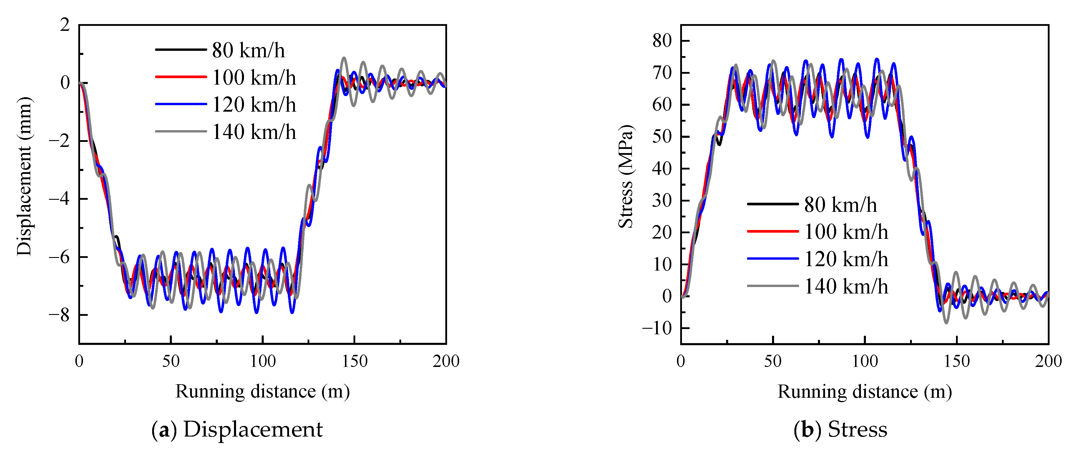
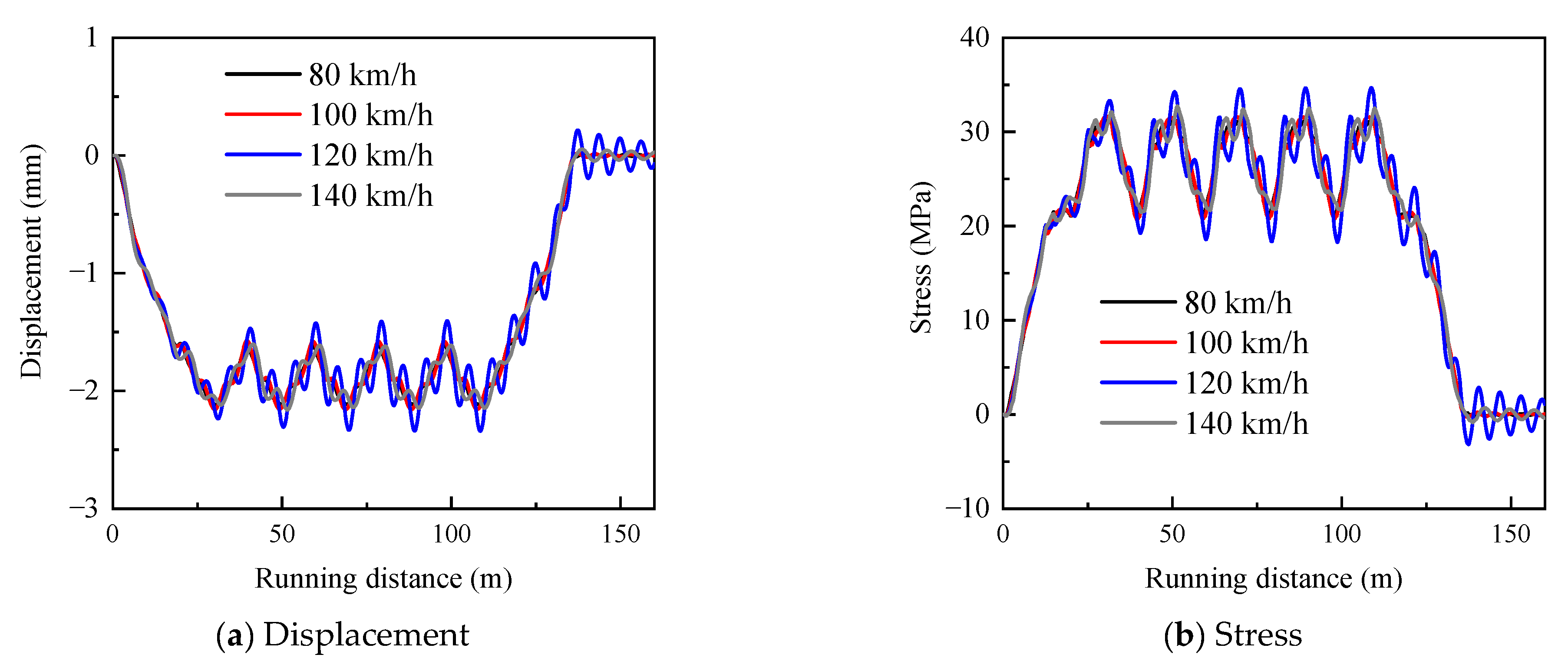
4.1. Time–History Curves

Under different vehicle speeds, the vertical displacement in the middle of the bridge span and the stress ergodic curve of the bottom longitudinal reinforcement of the 30 m-span bridge are calculated, as shown in Figure 5, where the abscissa represents the distance that the vehicle’s first wheel set passes through the left end of the bridge.

As can be seen from Figure 5a, the ergodic curve trend of bridge displacement response under different vehicle speeds is basically the same. When the vehicle speed is small (below 100 km/h), its dynamic deflection is relatively small, and its dynamic amplitude is small.

It can be found from Figure 5b that as the vehicle enters the bridge, the stress of the tensile reinforcement at the bottom of the girder gradually increases, peaking at around 70 MPa, and then presents vibrations of varying amplitudes as the vehicle continues to move forward (the amplitude is about 13 MPa below 100 km/h and about 20 MPa above 100 km/h), with multiple peaks and troughs. After the vehicle leaves the bridge, the tensile stress decreases gradually, and finally oscillates near 0 MPa and disappears gradually.

There are 10 peaks in both Figure 5a,b, as can be observed by comparing them. The number of peaks is related to the distribution of wheel sets, vehicle speed, and the bridge’s natural vibration characteristics, according to Liu et al. [28].

The vertical displacement at the bottom of the girder and the stress of the bottom longitudinal reinforcement of a 25 m-span bridge are depicted in Figure 6. The displacement in the middle of the span steadily grows as the car passes the bridge, and then shakes moderately, as seen in Figure 6a. When a car leaves the bridge, the bridge’s displacement progressively reduces, until it oscillates and decreases to near zero. Furthermore, when compared to Figure 5a, the peak displacement is minimal, with only five peaks and four troughs. The stress ergodic curve of the bottom longitudinal reinforcement gradually grows with the vehicle entering the bridge, then oscillates in the 20–35 MPa region, as shown in Figure 6b. Despite its small displacement in comparison to the 30 m bridge, its dynamic stress amplitude is comparable. The stress ergodic curve similarly has five peaks and four troughs.

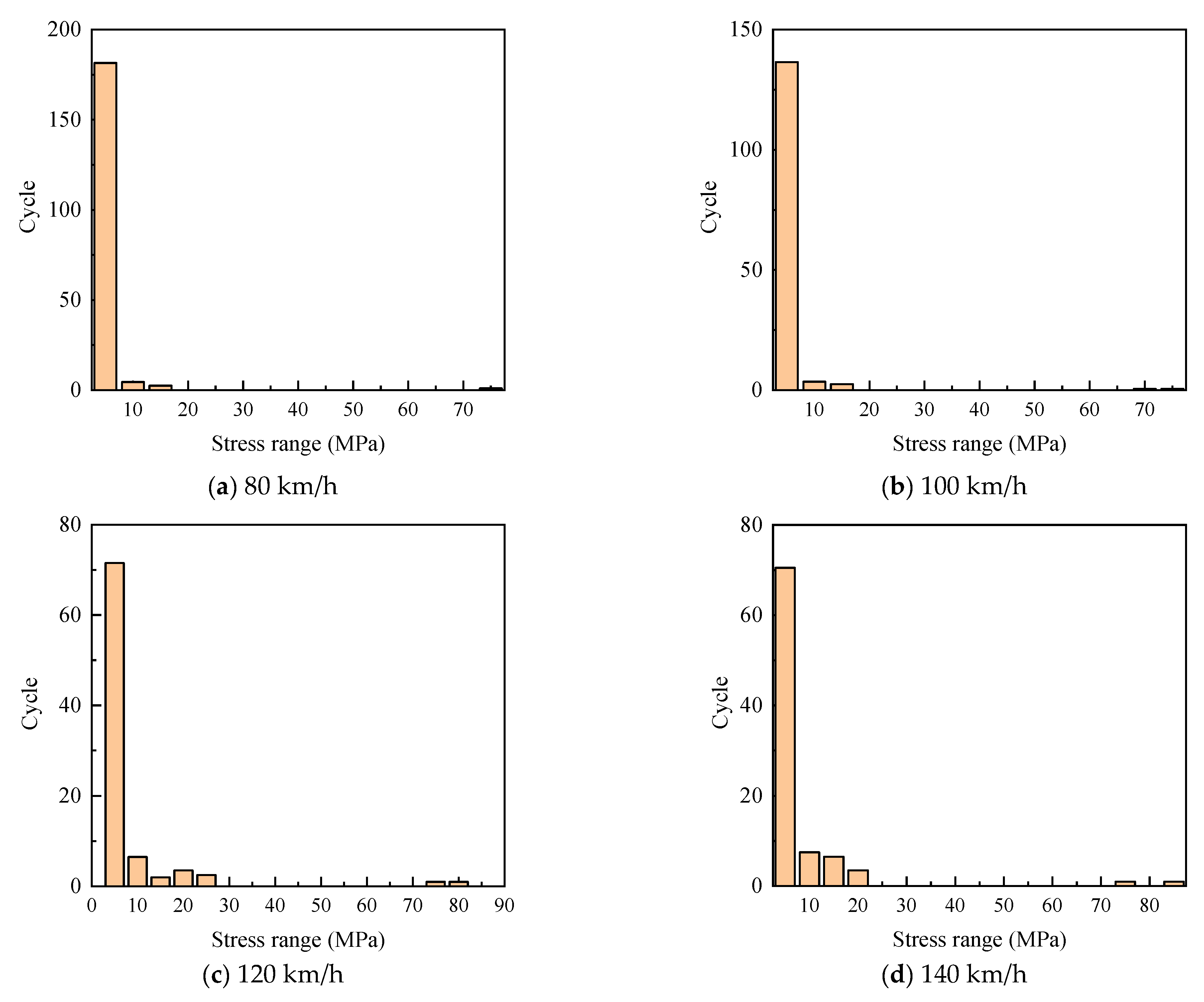
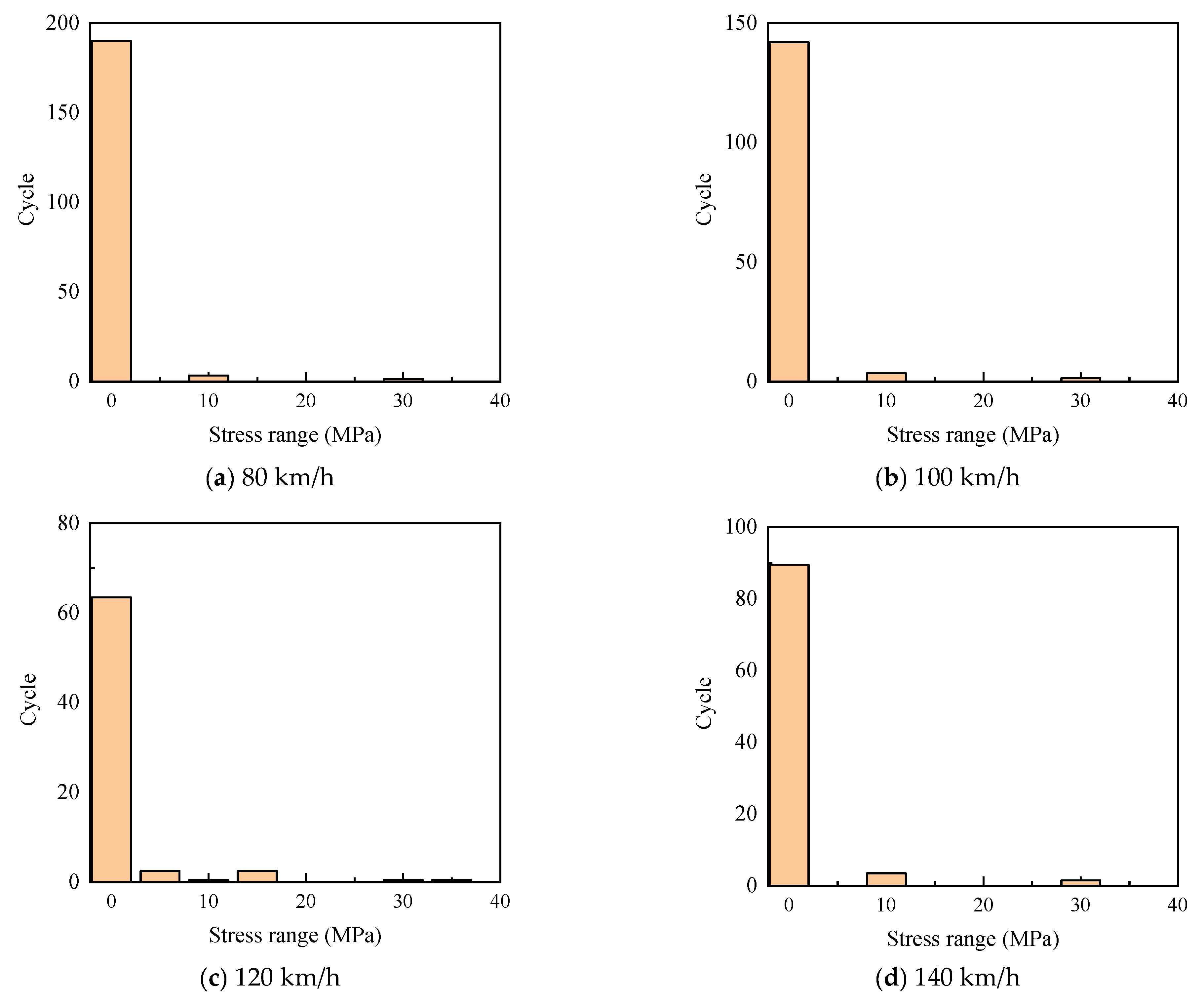
4.2. Stress Amplitude

The rain-flow counting approach can be used to calculate the stress amplitude and number of cycles after obtaining the reinforcement’s stress ergodic curve. The stress amplitude and number of cycles of the 30 m-span bridge are shown in Figure 7. The stress amplitude with the greatest number of cycles is found to be within 10 MPa at various vehicle speeds. The number of cycles of the stress amplitude above 10 MPa grows when the vehicle speed exceeds 100 km/h, whereas the number of cycles of the stress amplitude within 10 MPa decreases. There is no stress amplitude of 30 MPa to 65 MPa under varied vehicle speeds, and the number of cycles of stress amplitude greater than 30 MPa is less. This feature can also be found from the stress ergodic curve in Figure 5b.

The stress amplitude and cycle durations of a 25 m-span bridge are shown in Figure 8. The stress amplitude is mostly concentrated within 5 MPa at 80 km/h and 100 km/h, and the number of cycles is greater, reaching 180 and 140 times correspondingly, with a few cycles at 10 MPa and 30 MPa. When the vehicle is traveling at 120 km/h, the stress amplitude is widely distributed, and each stage has a set number of cycles. The distribution of stress amplitude and numbers of cycles when the vehicle speed is 120 km/h is comparable to that of 80 km/h and 100 km/h. Overall, vehicle speed has a significant impact on the stress amplitude and number of cycles, which has an impact on the bridge’s fatigue life.

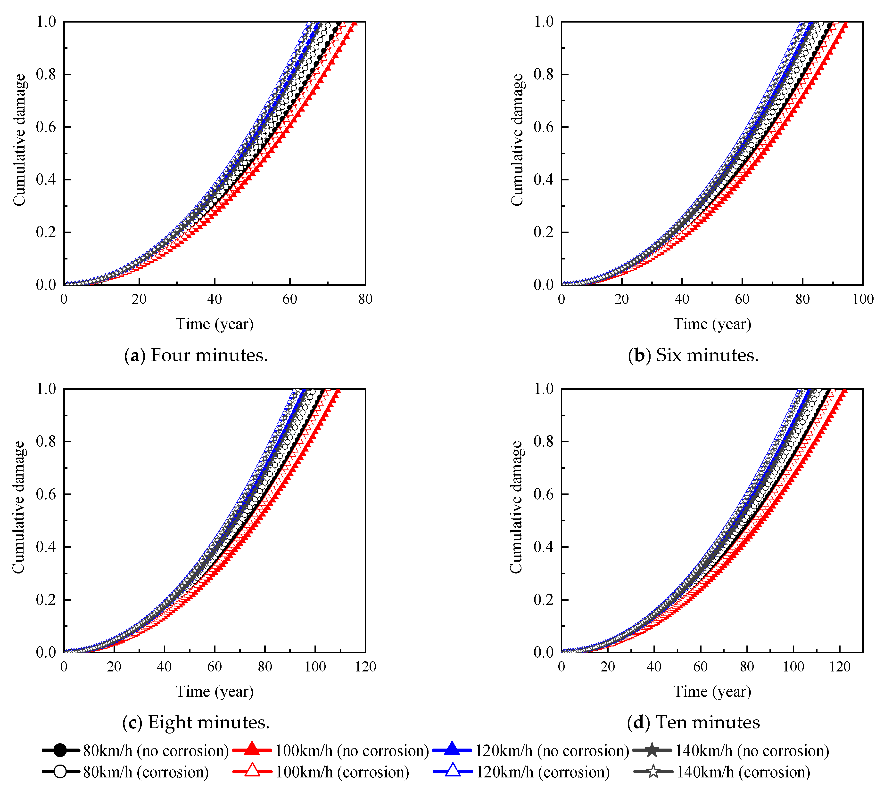
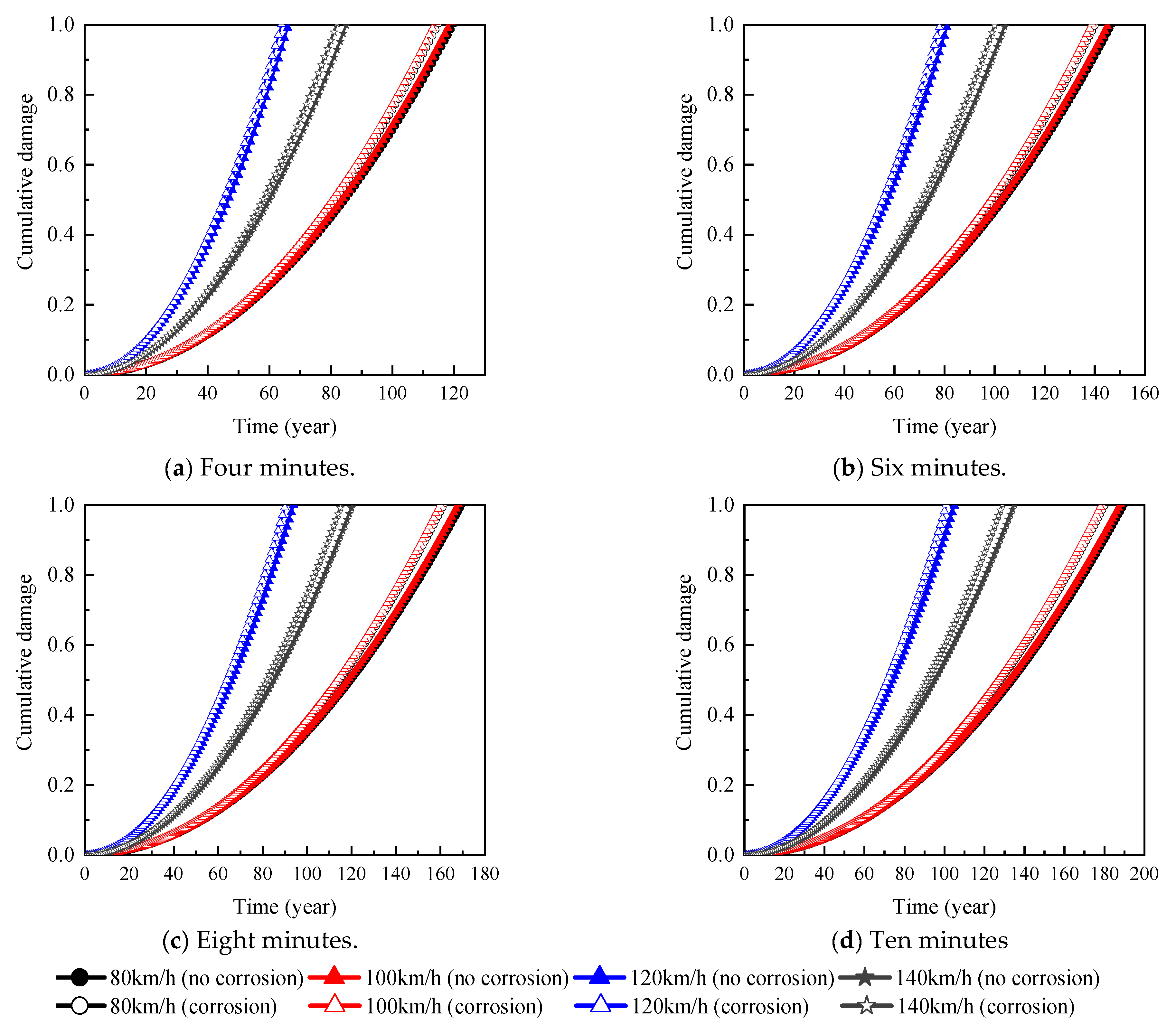
4.3. Cumulative Damage

The frequency with which the vehicle operates has a direct impact on the bridge structure’s fatigue life. The line runs from 6 a.m. to 22 p.m. for a total of 16 h, of which the interval between 6 a.m. to 7 a.m. and 21 a.m. to 22 a.m. is long, so the whole day is calculated as 15 h of operation. The vehicle intervals are 4, 6, 8, and 10 min, and the number of vehicles going through the single-track bridge is 24× operating hours/ interval = 225, 150, 113, and 90 times every day, the total number of vehicles traveling through the year is 365× daily operating train number = 82,125, 54,750, 41,063, and 32,850.

Figure 9 illustrates the cumulative damage of a 30 m-span bridge under various vehicle intervals, speeds, and whether corrosion fatigue is taken into account. When the cumulative damage value reaches 1, the bridge has reached the fatigue failure stage. The cumulative damage curve takes the shape of an inverted parabola in most cases. The cumulative damage of a bridge increases with the number of years it has been in operation, and the rate of growth increases gradually. The cumulative damage to the bridge diminishes as the vehicle operation interval increases throughout the same operation time.

Taking Figure 9a as an example (the damage curve law under different train intervals is similar), the growth rate of the cumulative damage curve considering corrosion fatigue is greater than ignoring cumulative damage at the same vehicle speed, in other words, the damage degree considering corrosion fatigue is greater than that ignoring corrosion fatigue at the same operation time, demonstrating the importance of considering corrosion fatigue. When comparing the cumulative damage fatigue curves for various vehicle speeds, it can be seen that the influence of vehicle speed on cumulative damage does not appear to be very consistent.

Figure 10 depicts the cumulative damage to a 25 m-span bridge under various vehicle intervals, speeds, and whether corrosion fatigue is taken into account. Similarly, the cumulative damage curve has an inverted parabola shape. The cumulative damage of the bridge increases as the number of operating years increases, and the rate of increase is progressive. The cumulative damage of the bridge reduces as the vehicle operation interval increases within the same operation time.

It can also be seen that vehicle speed has a significant impact on the fatigue cumulative damage curve of a 25 m-span bridge, but the influence law is not readily apparent. The cumulative damage curves corresponding to vehicle speeds of 80 km/h and 100 km/h, for example, are very similar, whereas the cumulative damage curves corresponding to 100 km/h and 120 km/h are very different. The cumulative damage curve corresponding to 120 km/h has a larger slope than that corresponding to 140 km/h over the same operation time, indicating that the bridge reaches fatigue failure faster when the speed is 120 km/h. This is because 120 km/h is closer to the third-order resonance speed (126 km/h) of the first-order natural vibration frequency of the bridge than 140 km/h [27]. The bridge resonates to a certain extent, resulting in the increase in the stress amplitude of the reinforcement, which can also be found in Figure 5. The bridge resonates to a certain extent, resulting in the increase in the stress amplitude of the reinforcement, which can also be found in Figure 5. In general, neglecting a material’s corrosion will result in a low-estimated damage degree.

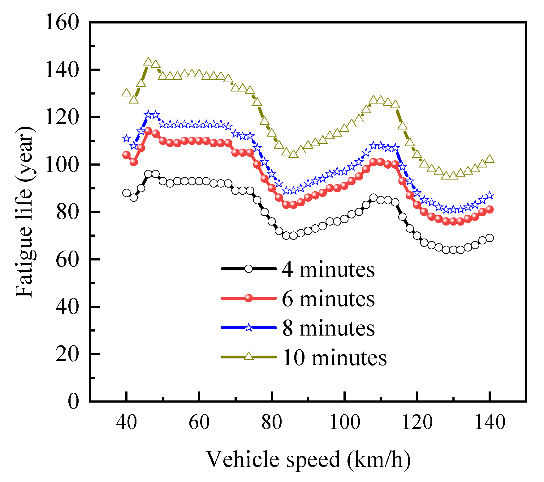
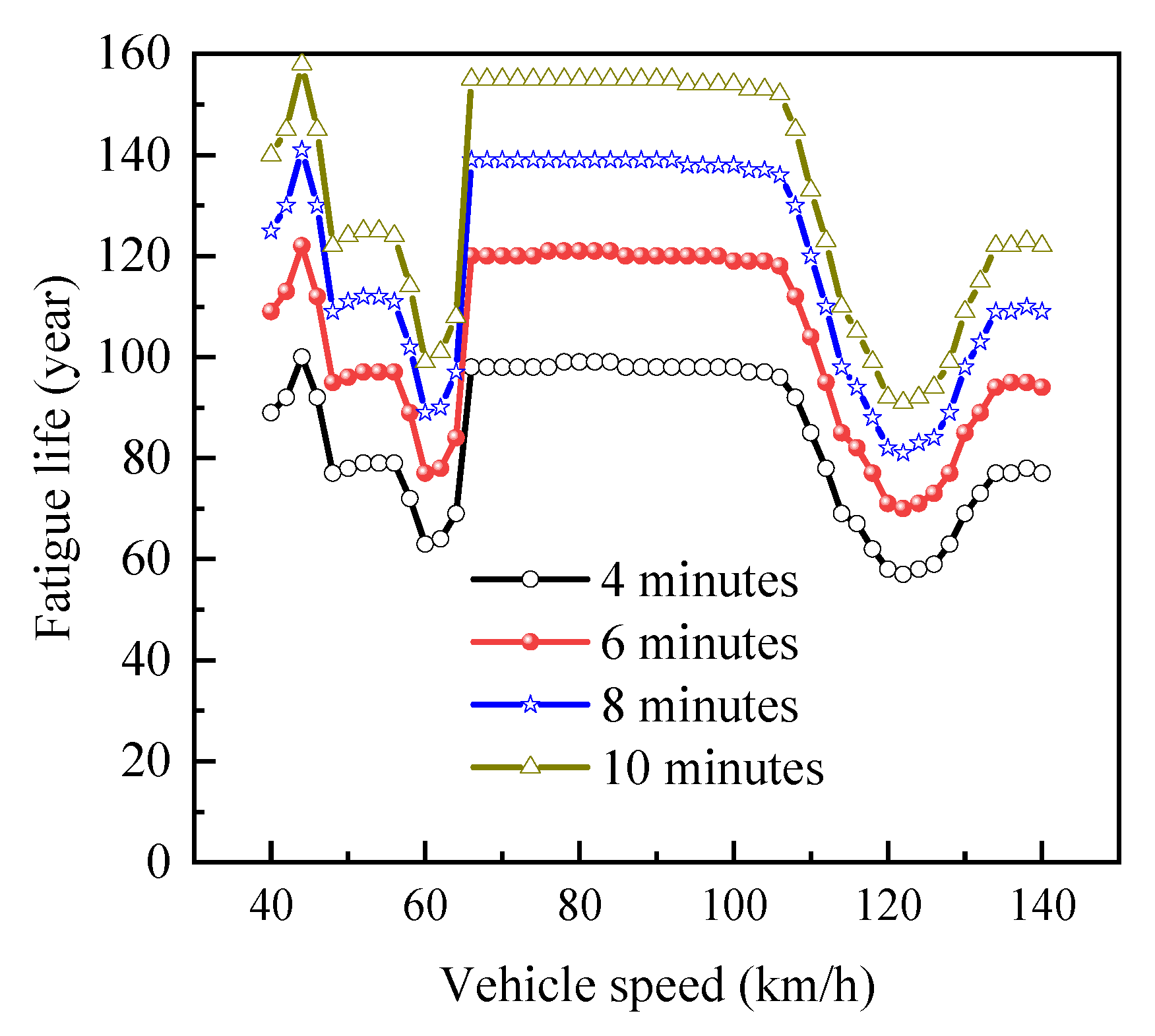
4.4. Fatigue Life Evaluation

The need to consider the environmental corrosion of the structure in the analysis of bridge fatigue life can be seen in Section 4.3. Furthermore, there is no clear law governing the effect of speed on the cumulative damage curve. The bridge fatigue life is calculated under different vehicle speeds and different train operation intervals in order to more systematically analyze the impact of vehicle operation speed on bridge fatigue life. The vehicle intervals are 4, 6, 8, and 10 min, respectively; the calculated train speed range is 40 km/h to 140 km/h, and the calculation is made once every 2 km/h.

The fatigue life of the 30 m-span bridge is depicted in Figure 11. The fatigue life of the bridge is found to increase as the vehicle interval increases at the same speed. With the increase in vehicle speed, the fatigue life goes through several stages at the same vehicle interval: (1) when the vehicle speed ranges from 40 km/h to 48 km/h, the fatigue life increases with the increase in vehicle speed; (2) when the vehicle speed is between 48 km/h and 76 km/h, the fatigue life reduces gradually; (3) when the vehicle speed ranges from 48 km/h to 76 km/h, the fatigue life decreases slowly with the increase in vehicle speed; (4) when the vehicle speed is between 86 and 116 km/h, the fatigue life grows rapidly; (5) when the vehicle speed is over 116 km/h, the fatigue life reduces at first, then increases as the vehicle speed increases. In terms of fatigue life, it is advised that the vehicle speed be kept within the operating speed range of about 115 km/h, and within 76 km during low-speed operation.

Figure 12 depicts the fatigue life of a bridge with a span of 25 m. It was also discovered that as the train interval increases at the same speed, the fatigue life of the bridge rises. The fatigue life curve of a 30 m-span bridge, which is primarily divided into three stages, is substantially different at the same interval: (1) when the vehicle speed is less than 60 km/h, the fatigue life reduces as the vehicle speed increases; (2) when the vehicle speed is 60 km/h to 78 km/h, the fatigue life increases fast as the vehicle speed increases; (3) when the vehicle speed is increased from 78 km/h to 116 km/h, the fatigue life drops, but the reduction range can be ignored; (4) with a vehicle speed greater than 116 km/h, the fatigue life increases first, then falls. From the perspective of fatigue life, it is recommended to control the speed within the range of 78 km/h to 116 km/h when driving on a 25 m-span bridge.

5. Conclusions

A vehicle–bridge system coupled model is developed to analyze the fatigue life of an intercity railway viaduct. FEM is utilized to build the bridge model, while multi-body dynamics is used to simulate the vehicle, and the wheel rail close fitting model is used to couple the two into a time-varying system. The bridge’s stress ergodic curve can be calculated, and the rain-flow counting method is then used to count the bridge stress amplitude and related cycle times of the vehicle passing by. The corrosion effect of the reinforcement and concrete components is also taken into account. The cumulative damage of the 30 m-span and 25 m-span bridges is evaluated at various vehicle speeds, operating intervals, and whether or not material corrosion is taken into account. Finally, the bridge’s fatigue life is assessed, and the following findings are drawn:

(1)

The vehicle speed has a significant impact on the bridge’s displacement and stress ergodic curve; when the vehicle passes through different span bridges, the displacement and ergodic curve trends are drastically different, with 30 m-span bridges having higher peak displacement and stress than 25 m-span bridges. However, the dynamic stress amplitudes of the two types of spans are close.

(2)

Vehicle speed has a significant impact on the stress amplitude and cycle times, with the majority of cycles concentrated in the small stress amplitude stage.

(3)

According to cumulative curves, material corrosion should be considered, and there is no evident law governing the impact of vehicle speed on the cumulative damage curve.

(4)

The bridge fatigue life is inconsistent at different speeds, and the fatigue life of bridges with different spans is vastly different. Based on this, the recommended vehicle speed is proposed from the standpoint of fatigue life. For bridges with a 30 m span, it is recommended that the speed be kept between 115 km/h and 70 km/h; for bridges with a 25 m span, the speed should be kept between 78 km/h and 116 km/h.

(5)

Under the long-term fatigue load, the structure will have stiffness degradation, which will increase the stress amplitude of reinforcement and concrete. In addition, the interlayer components may be damaged. How to reasonably consider the degradation and damage is a problem that needs to be paid attention to in the future.

References

1. Sheng, X.-W.; Zheng, W.-Q.; Zhu, Z.-H.; Qin, Y.-P.; Guo, J.-G. Full-scale fatigue test of unit-plate ballastless track laid on long-span cable-stayed bridge. Constr. Build. Mater. 2020, 247, 118601. [Google Scholar] [CrossRef]
2. Zhou, L.-Y.; Zhao, L.; Mahunon, A.D.; Zhang, Y.-Y.; Li, H.-Y.; Zou, L.-F.; Yuan, Y.-H. Experimental study on stiffness degradation of CRTS II ballastless track-bridge structural system under fatigue train load. Constr. Build. Mater. 2021, 283, 122794. [Google Scholar] [CrossRef]
3. Zhao, L.; Zhou, L.; Yu, Z.; Mahunon, A.D.; Peng, X.; Zhang, Y. Experimental study on CRTS II ballastless track-bridge structural system mechanical fatigue performance. Eng. Struct. 2021, 244, 112784. [Google Scholar] [CrossRef]
4. Zeng, Z.; Wang, J.; Shen, S.; Li, P.; Abdulmumin Ahmed, S.; Wang, W. Experimental study on evolution of mechanical properties of CRTS III ballastless slab track under fatigue load. Constr. Build. Mater. 2019, 210, 639–649. [Google Scholar] [CrossRef]
5. Zhu, S.; Wang, M.; Zhai, W.; Cai, C.; Zhao, C.; Zeng, D.; Zhang, J. Mechanical property and damage evolution of concrete interface of ballastless track in high-speed railway: Experiment and simulation. Constr. Build. Mater. 2018, 187, 460–473. [Google Scholar] [CrossRef]
6. Song, L.; Cui, C.; Liu, J.; Yu, Z.; Jiang, L. Corrosion-fatigue life assessment of RC plate girder in heavy-haul railway under combined carbonation and train loads. Int. J. Fatigue 2021, 151, 106368. [Google Scholar] [CrossRef]
7. Cui, C.; Song, L.; Liu, J.; Yu, Z. Corrosion-Fatigue Life Prediction Modeling for RC Structures under Coupled Carbonation and Repeated Loading. Mathematics 2021, 9, 3296. [Google Scholar] [CrossRef]
8. Kang, C.; Schneider, S.; Wenner, M.; Marx, S. Experimental investigation on rail fatigue resistance of track/bridge interaction. Eng. Struct. 2020, 216, 110747. [Google Scholar] [CrossRef]
9. Zhu, Z.; Gong, W.; Wang, K.; Liu, Y.; Davidson, M.T.; Jiang, L. Dynamic effect of heavy-haul train on seismic response of railway cable-stayed bridge. J. Cent. South Univ. 2020, 27, 1939–1955. [Google Scholar] [CrossRef]
10. Liu, X.; Jiang, L.; Lai, Z.; Xiang, P.; Chen, Y. Sensitivity and dynamic analysis of train-bridge coupled system with multiple random factors. Eng. Struct. 2020, 221, 111083. [Google Scholar] [CrossRef]
11. Liu, X.; Jiang, L.; Xiang, P.; Lai, Z.; Feng, Y.; Cao, S. Dynamic response limit of high-speed railway bridge under earthquake considering running safety performance of train. J. Cent. South Univ. 2021, 28, 968–980. [Google Scholar] [CrossRef]
12. Liu, X.; Xiang, P.; Jiang, L.; Lai, Z.; Zhou, T.; Chen, Y. Stochastic Analysis of Train–Bridge System Using the Karhunen–Loéve Expansion and the Point Estimate Method. Int. J. Struct. Stab. Dyn. 2020, 20, 2050025. [Google Scholar] [CrossRef]
13. Malveiro, J.; Sousa, C.; Ribeiro, D.; Calçada, R. Impact of track irregularities and damping on the fatigue damage of a railway bridge deck slab. Struct. Infrastruct. Eng. 2018, 14, 1257–1268. [Google Scholar] [CrossRef]
14. Li, H.; Frangopol, D.M.; Soliman, M.; Xia, H. Fatigue reliability assessment of railway bridges based on probabilistic dynamic analysis of a coupled train-bridge system. J. Struct. Eng. 2016, 142, 04015158. [Google Scholar] [CrossRef]
15. Wang, C.; Zhang, J.; Tu, Y.; Sabourova, N.; Grip, N.; Blanksvärd, T.; Elfgren, L. Fatigue assessment of a reinforced concrete railway bridge based on a coupled dynamic system. Struct. Infrastruct. Eng. 2020, 16, 861–879. [Google Scholar] [CrossRef]
16. Xu, L.; Liu, H.; Yu, Z. A coupled model for investigating the interfacial and fatigue damage evolution of slab tracks in vehicle-track interaction. Appl. Math. Model. 2022, 101, 772–790. [Google Scholar] [CrossRef]
17. Rageh, A.; Eftekhar Azam, S.; Linzell, D.G. Steel railway bridge fatigue damage detection using numerical models and machine learning: Mitigating influence of modeling uncertainty. Int. J. Fatigue 2020, 134, 105458. [Google Scholar] [CrossRef]
18. Li, H.; Wu, G. Fatigue Evaluation of Steel Bridge Details Integrating Multi-Scale Dynamic Analysis of Coupled Train-Track-Bridge System and Fracture Mechanics. Appl. Sci. 2020, 10, 3261. [Google Scholar] [CrossRef]
19. Reagan, D.; Sabato, A.; Niezrecki, C. Feasibility of using digital image correlation for unmanned aerial vehicle structural health monitoring of bridges. Struct. Health Monit. 2018, 17, 1056–1072. [Google Scholar] [CrossRef]
20. Wang, H.; Chang, L.; Markine, V. Structural Health Monitoring of Railway Transition Zones Using Satellite Radar Data. Sensors 2018, 18, 413. [Google Scholar] [CrossRef] [Green Version]
21. Fan, X.P.; Liu, Y.F. New Dynamic Prediction Approach for the Reliability Indexes of Bridge Members Based on SHM Data. J. Bridge Eng. 2018, 23, 06018004. [Google Scholar] [CrossRef]
22. Xiang, P.; Wei, M.; Sun, M.; Li, Q.; Jiang, L.; Liu, X.; Ren, J. Creep Effect on the Dynamic Response of Train-Track-Continuous Bridge System. Int. J. Struct. Stab. Dyn. 2021, 21, 2150139. [Google Scholar] [CrossRef]
23. Papadakis, V.; Vayenas, C.; Fardis, M. Fundamental Modeling and Experimental Investigation of Concrete Carbonation. ACI Mater. J. 1991, 88, 363–373. [Google Scholar]
24. GB/T 51355-2019; Standard for Durability Assessment of Existing Concrete Structures. China Architecture & Building Press: Beijing, China, 2019. (In Chinese)
25. Li, X.; Wang, Z.; Ren, W. Time-dependent reliability assessment of reinforced concrete bridge under fatigue loadings. China Railw. Sci. 2009, 30, 49–53. [Google Scholar]
26. Miner, M.A. Cumulative Damage in Fatigue. J. Appl. Mech. 1945, 12, A159–A164. [Google Scholar] [CrossRef]
27. Wang, J.; Cui, C.; Liu, X.; Wang, M. Dynamic Impact Factor and Resonance Analysis of Curved Intercity Railway Viaduct. Appl. Sci. 2022, 12, 2978. [Google Scholar] [CrossRef]
28. Liu, X.; Jiang, L.; Xiang, P.; Lai, Z.; Liu, L.; Cao, S.; Zhou, W. Probability analysis of train-bridge coupled system considering track irregularities and parameter uncertainty. Mech. Based Des. Struct. Mach. 2021, 1–18. [Google Scholar] [CrossRef]
Figure 1. Vehicle–bridge coupled system.
Mathematics 10 01663 g001
Figure 2. Validation of numerical model.
Mathematics 10 01663 g002
Figure 3. Rain-flow counting method.
Mathematics 10 01663 g003
Figure 4. Section size of girder (Unit: cm).
Mathematics 10 01663 g004
Figure 5. Time–history response curves of midspan of 30-m bridge.
Mathematics 10 01663 g005
Figure 6. Time–history response curves of midspan of 25 m-span bridge.
Mathematics 10 01663 g006
Figure 7. Stress range of steel rebar of 30 m-span bridge.
Mathematics 10 01663 g007
Figure 8. Stress range of steel rebar of 25 m-span bridge.
Mathematics 10 01663 g008
Figure 9. The cumulative damage of 30 m-span bridge.
Mathematics 10 01663 g009
Figure 10. The cumulative damage of 25 m-span bridge.
Mathematics 10 01663 g010
Figure 11. Fatigue of 30 m bridge under various vehicle speed.
Mathematics 10 01663 g011
Figure 12. Fatigue of 25 m-span bridge under various vehicle speed.
Mathematics 10 01663 g012