Measuring Variable Importance in Generalized Linear Models for Modeling Size of Loss Distributions

Abstract

Predictive modeling is a critical technique in many real-world applications, including auto insurance rate-making and the decision making of rate filings review for regulation purposes. It is also important in predicting financial and economic risk in business and economics. Unlike testing hypotheses in statistical inference, results obtained from predictive modeling serve as statistical evidence for the decision making of the underlying problem and discovering the functional relationship between the response variable and the predictors. As a result of this, the variable importance measures become an essential aspect of helping to better understand the contributions of predictors to the built model. In this work, we focus on the study of using generalized linear models (GLM) for the size of loss distributions. In addition, we address the problem of measuring the importance of the variables used in the GLM to further evaluate their potential impact on insurance pricing. In this regard, we propose to shift the focus from variable importance measures of factor levels to factors themselves and to develop variable importance measures for factors included in the model. Therefore, this work is exclusively for modeling with categorical variables as predictors. This work contributes to the further development of GLM modeling to make it even more practical due to this added value. This study also aims to provide benchmark estimates to allow for the regulation of insurance rates using GLM from the variable importance aspect.

1. Introduction

In auto insurance, many risk factors are categorical, such as the type of use, coverage, territory and driver record, to name a few. Some risk factors are numerical, but they are often converted into a grouped variable for pricing as they significantly improve the model prediction accuracy [1,2]. For instance, drivers’ ages are often converted into an age group, and the number of years of driving experiences is also grouped into different categories. When using predictive modeling, the model often captures the effect of the factor level within each categorical factor rather than the factor itself, such as in generalized linear models (GLM). In auto insurance pricing, these estimates of impact from factor levels are used to derive the relative risk measures of those risk factor levels and are eventually used as inputs of a pricing algorithm used by insurance companies. However, some decisions are made in risk management based on the considered risk factors, and not their associated factor levels. Therefore, it is important to focus on studying more dominant risk factors through some quantitative measures. This can be achieved by shifting the focus from factor levels to factors themselves. This may be interpreted as a dimension reduction problem in statistics. As a result of this, one has to further evaluate the factor effect, which is often carried out by looking at the effect size for each factor using t-test statistics or an ANOVA table [3,4]. This study emphasizes how to measure the importance of risk factors used in auto insurance rate regulation, illustrated by using the size of loss distributions.

On the other hand, any predictive modeling requires information on what factors to include, which is often referred to as variable selection [5]. In a real-world application, massive data that contain many variables often occur for some given problems. Therefore, dimension reduction in input factors for a predictive model is required, and this is often carried out by variable selection [6,7] or measuring the importance of considered variables, with or without a model involved [8,9,10]. The variable selection is appropriate for massive input factors, whereas measuring variable importance is more suitable for small-to-medium-sized input factors. In insurance rate regulation, only major factors are considered, such as the driver class, driving record, territory and coverage. Other factors may also affect the results, such as the accident years and reporting years, but they may be considered minor. The study focusing on risk factors used in rate regulation is different from the predictive modeling of insurance loss conducted by an individual company, where all relevant risk factors are being considered. This difference allows us to focus on predictive models that are more interpretable, such as multiple linear regression models, generalized linear models, generalized additive models and other interpretable machine learning models [11,12,13].

The study of big data for decision making is rapidly growing because the use of big data often provides more accurate information so that the decision making is more reliable than the case using a small data set [14,15,16]. From the statistical perspective, the greater the amount of data used for computing statistics, the better the estimate of the unknown parameters. This is particularly true in insurance rate regulation, so industry-level data are used. Of course, big data do not just indicate the enormous data volume; they also imply a high level of data complexity. One may need to see that, among all factors considered in the model, what the measures in terms of their importance to model buildings are, mainly when factors are categorical and consist of many different factor levels. Therefore, the investigation of suitable approaches to measuring variable importance in insurance pricing has become an emerging research area and has attracted significant attention in machine learning for insurance [11,17,18,19].

Traditionally, auto insurance pricing is based on calculating the relativity of each level within a given factor. After obtaining the relativity of each level of a given factor for all risk factors, the relative premium level (i.e., without considering the basis) for a given risk class is then determined by multiplying each relativity of a given factor level across all risk factors considered. This is referred to as a multiplicative pricing algorithm, which insurance companies are currently using [20,21]. The result obtained from the multiplication of relativities of all risk levels is then multiplied by the base premium to calculate the actual premium for a given class. This multiplicative pricing based on the relativity of risk level assumes that all risk factors are equally important in calculating the overall risk relativity. Only essential factors are considered in the predictive modeling of loss cost in rate regulation. However, the contribution to explaining the response variable variation due to each factor may not be the same. Therefore, when a predictive modeling approach is taken to derive the relativity, such as generalized linear models, it is crucial to know which factors are the more dominant within all factors considered for rate regulation purposes. This can help us to better understand the effect of the factors on the major components of insurance pricing [22].

This work focuses on measuring the variable importance associated with the size of loss distributions from the automobile statistical plan. We use aggregated claim counts and aggregated loss amounts summarized by the different dimensions of risk factors used for regulation purposes. We aim to see which risk factor influences the loss amounts and counts the most when GLM is used as a predictive model. That is to say, which factor is the most dominant in the loss amounts and claim counts. Our contribution is to the development of new variable importance measures for GLM. This is particularly novel for better decision-making of rate regulation since GLM is widely used for insurance pricing and the predictive modeling of insurance loss. We also investigate if the dominant factor influencing the claim counts is the same as the dominant factor influencing the loss amounts. The risk factors considered are the territory, size of loss, insurance coverage, accident year and reporting year.

The rest of this paper is organized as follows. In Section 2, we review the related work that provides background and current research similar to this work. In Section 3, we discuss the proposed methods of how to measure the variable importance in GLM. We provide a detailed mathematical description of how the proposed method is developed. In Section 4, an analysis of the size of loss data and a summary of the main results are presented. Finally, we conclude our findings and provide further remarks in Section 5.

2. Related Work

This section discusses related work on measuring variable importance for a predictive model. We first discuss the sensitivity-based approach used to evaluate the variable importance in non-linear regression problems such as artificial neural network models. We then discuss the generalized additive models, which can also be used to address the variable importance problem. Finally, we reviewed other related model-specific variable importance measure approaches.

2.1. Evaluating Importance of Risk Factors in Non-Linear Regression Models via Sensitivity Analysis

Consider the following general form of a non-linear regression problem

$$\begin{array}{c}\hfill y=f(x_1,x_2,\dots ,x_D)+ϵ,\end{array}$$

(1)

where $x_1,x_2,\dots ,x_D$ are risk factors, y is the response variable and f is a non-linear function, either parametric or non-parametric. To further investigate the importance of the risk factors, the Taylor series expansion of y at the first order, which is given as follows, can be conducted:

$$\begin{array}{c}\hfill \Delta y=f(x_1+\Delta x_1,x_2+\Delta x_2,\dots ,x_D+\Delta x_D)\approx \frac{\partial f}{\partial x_1}\Delta x_1+\frac{\partial f}{\partial x_2}\Delta x_2+\dots \frac{\partial f}{\partial x_D}\Delta x_D.\end{array}$$

(2)

Here, $\frac{\partial f}{\partial x_i}$ is referred to as the sensitivity coefficient of $x_i$ and may be used to represent the effect of risk factor $x_i$ when holding other variables constant. However, we may not have the explicit functional form of $f(x_1,x_2,\dots ,x_D)$, such as the artificial neural network (ANN), and deriving the sensitivity coefficient in a closed-form is impossible. A possible solution for this is to use Lek’s profile method [23] to conduct a sensitivity analysis. Lek’s profile approach evaluates the effect of each input variable on the output variable by holding the remaining explanatory variables constant. The constant values of unevaluated explanatory variables can be at different quantiles (e.g., we use minimum, 50th percentile and maximum) in this work. It is implemented by creating a matrix that contains constant values (e.g., at the median) for all remaining explanatory variables constant, while the variable of interest is sorted in ascending order. This data matrix is then used to predict the response variable using a fitted modelm, such as ANN. This process is then repeated for each input variable to obtain all response curves [24].

2.2. Generalized Additive Models

A second possible approach to determine the variable importance measure for the given factor is to use a generalized additive model, in which, the model can be specified as follows:

$$\begin{array}{c}\hfill y={\beta }_0+\sum _{i=1}^D{\beta }_j{f}_j\left(x_j\right)+ϵ,\end{array}$$

(3)

where $f_j$ are some linear or non-linear functions. This allows us to model the relationship between $x_j$ by going beyond the standard linear regression. In the GAM, the variable $x_j$ can be either categorical or numerical variables. The functions $f_j$ can be the spline functions, such as cubic spline. Other possible function forms, such as polynomial or non-parametric functions, are also common. In the GAM setting, we estimate the contribution of component $f_j\left(x_j\right)$, which is the coefficient ${\beta }_j$. Variable importance measures are then given by t-values of the coefficients or the reciprocal of the p-value of the t-test in testing the significance of coefficients. They can also be defined using the risk relativity of each factor. Obtaining the risk relativity from GAM is similar to the GLM, discussed in the next section. As we can see from the model setting shown in Equation (3), the GAM method is more appropriate for the numerical type of variable, including the ordinal scale of the numerical factor. This is because of the imposed functionality by $f_j(·)$. However, for a categorical variable, we are facing the same problem as the one we will see in the GLM setting. If importance is measured for a factor, we must consider an approach that can summarize the estimate from the factor levels. The common characteristic of the model-based variable importance measure, including the sensitivity measure of the variable and the GAM approach, tries to capture the association between the response variable and a function or a mathematical operation of $x_j$.

2.3. Other Model Specific Approaches

In machine learning, decision-tree-based approaches are often used to obtain variable importance measures by capturing the effect of the considered variable to the model prediction performance. This work also compares results obtained from our proposed method to the tree-based approach, including single decision tree, random forest and XGBoosting. The predictor variables are split in a binary decision tree at each node to produce two homogeneous groups. Choosing a predictor is determined by maximizing some measure of improvements, such as a reduction in mean square errors or Gini impurity measure. The variable importance of predictor X becomes the sum of the squared improvements in overall internal nodes of the tree, for which, X was chosen as the splitting variable [25]. Random forest is an ensemble method that uses many different decision trees. The variable importance measure can be obtained by taking the average measures of variable importance obtained from each decision tree. Due to the re-sampling process, random forest often offers a more stable and reliable method for measuring variable importance than other tree-based methods [26]. Boosting applied to decision trees determines the weight value to construct a linear combination of decision trees. Similar to random forest, the variable importance measure is computed based on the averaged squared improvement over all of the internal nodes of the tree. Other model-based methods may include the linear model and non-linear regression methods, such as an artificial neural network. However, linear and neural network models produce variable importance measures for factor levels, and not a single categorical factor. Therefore, within the scope of the work, it becomes less valuable.

3. Materials and Methods

3.1. Data

In this study, we focus on a large loss data set from the Insurance Bureau of Canada (IBC). IBC is an organization that is responsible for insurance data collection and its data reporting. This data set consists of summarized claim counts and loss amounts by different loss levels. The size-of-loss is grouped into different bins and the aggregated value of claim counts and loss amounts are reported by different bins. The response variables are of the numerical type, whereas all risk factors are considered to be categorical. These aggregated claim counts and loss amounts were also summarized by major insurance coverages, i.e., bodily injury (BI) and accident benefit (AB), by different accident years, by different data reporting years and by different territories, i.e., urban and rural. We define claim counts and loss amounts as response variables, and coverages, accident years, reporting years, territories and loss levels as risk factors taking different levels. More specifically, coverages have two levels, accident benefit (AB) and bodily injury (BI); there are rolling five accident years for each statistical report year, and the statistical data reporting is conducted annually (in this work, we have data for two reporting years). Territories have two levels, urban and rural. Lastly, the size-of-loss contains 24 different groups with unequal lengths.

Table 1. The size of loss distribution in terms of claim frequency, claim amount, expense and aggregate loss for the combination of urban region, AB coverage and 2014 accident year for the 2014 report year.

Coverage: AB
Period	2014
Trended to:	2010.67	2014.75		1 October 2014
Annual Trend	7.20%	5.10%
Trend Factor	1.012590732
LDF:	1.738307595
		# of Claims	Incurred losses	Incurred expenses
Lower Limit	Upper Limit	Freq.	Total Loss	Total Exp.	Loss + Exp	Trended Ultimate
						Losses and Exp
$0		5247	-	$5,424,523	$5,424,523	$9,548,214
$1	$1000	13,846	$4,898,741	$3,192,136	$8,090,877	$14,241,514
$1001	$2000	11,695	$17,868,052	$4,377,219	$22,245,271	$39,155,996
$2001	$3000	17,363	$40,610,201	$2,499,151	$43,109,352	$75,880,830
$3001	$4000	20,330	$70,850,254	$8,973,969	$79,824,223	$140,506,131
$4001	$5000	16,022	$73,492,385	$4,040,104	$77,532,489	$136,472,234
$5001	$10,000	31,074	$238,908,273	$14,664,087	$253,572,360	$446,336,587
$10,001	$15,000	13,499	$168,725,634	$9,305,771	$178,031,405	$313,369,839
$15,001	$20,000	8264	$145,758,931	$7,036,983	$152,795,914	$268,950,476
$20,001	$25,000	4354	$97,821,028	$5,409,368	$103,230,396	$181,705,540
$25,001	$30,000	3453	$94,941,271	$4,261,494	$99,202,765	$174,616,128
$30,001	$40,000	4068	$141,599,160	$6,328,065	$147,927,225	$260,380,638
$40,001	$50,000	2144	$96,215,854	$4,933,842	$101,149,696	$178,043,104
$50,001	$75,000	2308	$139,797,760	$6,917,330	$146,715,090	$258,247,045
$75,001	$100,000	1029	$88,618,550	$3,963,795	$92,582,345	$162,962,903
$100,001	$150,000	684	$81,987,834	$3,478,170	$85,466,004	$150,436,761
$150,001	$200,000	173	$29,586,463	$1,019,194	$30,605,657	$53,871,899
$200,001	$300,000	149	$36,506,839	$830,420	$37,337,259	$65,720,825
$300,001	$400,000	84	$29,606,699	$430,171	$30,036,870	$52,870,723
$400,001	$500,000	69	$31,530,518	$759,586	$32,290,104	$56,836,852
$500,001	$750,000	63	$38,287,083	$413,871	$38,700,954	$68,121,193
$750,001	$1,000,000	34	$31,215,367	$467,750	$31,683,117	$55,768,438
$1,000,001	$2,000,000	54	$75,090,254	$862,952	$75,953,206	$133,692,390
$2,000,000	$9,999,999	14	$35,584,904	$559,828	$36,144,732	$63,621,746

shows an example of such a data set for the combination of AB coverage, 2014 report year, 2014 accident year and urban region. Claim counts and loss amounts are trended and developed to the ultimate level. The key characteristics of this type of datum are the grouped nature and highly right-skewed distributions for both loss amounts and claim counts.

3.2. Specifying a Multiple Linear Regression Model for Categorical Risk Factors

A sensitivity study by a linearly approximated model tackles the variable importance problem in a non-linear model. However, the approach requires a fitted non-linear model, which is often a black box. The study of variable importance problems associated with these black-box models is to better understand or interpret the model used. Now, we turn our focus to interpretable statistical models.

As one of the most important interpretable statistical models, multiple linear regression (MLR) has been widely used for analyzing data in many fields of application, including business and economics. In this work, the MLR model is used to establish the relationship between the risk factors we considered and the response variables, claim counts, claim amount or average loss per claim count. We denote $Y_1$ as the claim count, $Y_2$ as the claim amount and $Y_3$ as the average loss per claim count. We further denote coverages, territories, loss levels, accident years and report years as variables $X_1$, $X_2$, $X_3$, $X_4$, $X_5$. $X_1$ has two levels, bodily injury (BI) and accident benefit (AB); $X_2$ includes urban and rural; $X_3$ contains 24 loss levels; $X_4$ contains five accident years; and $X_5$ has two levels, current report year and the last report year. Since all risk factors are categorical, we must define them as dummy variables. Thus, we define the following dummy variables:

$$X_1=\left\{\begin{array}{cc}1\hfill & \mathrm{if}\mathrm{it}\mathrm{is}\mathrm{BI}\hfill \\ 0\hfill & \mathrm{otherwise}\hfill \end{array}\right.;X_2=\left\{\begin{array}{cc}1\hfill & \mathrm{if}\mathrm{it}\mathrm{is}\mathrm{Rural}\hfill \\ 0\hfill & \mathrm{otherwise}\hfill \end{array}\right.;X_3^i=\left\{\begin{array}{cc}1\hfill & \mathrm{if}\mathrm{it}\mathrm{is}(i+1)\mathrm{th}\mathrm{loss}\mathrm{level}\hfill \\ 0\hfill & \mathrm{otherwise}\hfill \end{array}\right.,\mathrm{for}i=1,\dots 23.$$

$$X_4^i=\left\{\begin{array}{cc}1\hfill & \mathrm{if}\mathrm{it}\mathrm{is}(i+1)\mathrm{acident}\mathrm{year}\hfill \\ 0\hfill & \mathrm{otherwise}\hfill \end{array}\right.\mathrm{for}i=1,\dots 4;X_5=\left\{\begin{array}{cc}1\hfill & \mathrm{if}\mathrm{it}\mathrm{is}\mathrm{current}\mathrm{report}\mathrm{year}\hfill \\ 0\hfill & \mathrm{otherwise}\hfill \end{array}\right..$$

The way we define the dummy variables implies that we take the combination of AB, urban, zero loss, first accident year and the last reporting year as a basis level. The objective of regression modeling is to estimate the coefficient of the risk level within the given factor, which can be interpreted as the effect compared to the basis level. Therefore, the regression model for $Y_j$, where $j=1,2,3$, can be specified as follows:

$$\begin{array}{ccc}\hfill E\left(Y_j\right)& =& {\beta }_0^{\left(j\right)}+{\beta }_1^{\left(j\right)}{X}_1+{\beta }_2^{\left(j\right)}{X}_2+\sum _{i=1}^{23}{\beta }_{i+2}^{\left(j\right)}{X}_3^i+\sum _{i=1}^4{\beta }_{25+i}^{\left(j\right)}{X}_4^i+{\beta }_{29}^{\left(j\right)}{X}_5\hfill \end{array}$$

(4)

or, in the matrix notation,

$$\begin{array}{c}\hfill E\left(Y_j\right)=\mathbf{X}{{\beta }^{\left(j\right)}}^{\top },\end{array}$$

(5)

where $\mathbf{X}$ = $[1,X_1,X_2,X_3^1,\dots ,X_3^{23},X_4^1,\dots ,X_4^4,X_5]$, and ${\beta }^{\left(j\right)}$ = $[{\beta }_0^{\left(j\right)},{\beta }_1^{\left(j\right)},{\beta }_2^{\left(j\right)},\dots ,{\beta }_{29}^{\left(j\right)}]$.

3.3. Generalized Linear Models

In MLR, the response variable is often assumed to follow a normal (i.e., Gaussian) distribution, and the variance is assumed to be constant. However, these assumptions may not be easily satisfied by the data from real-world applications. The generalized linear models (GLM) extend the assumption of the Gaussian family to a more general case, called the exponential family distribution [27]. Furthermore, instead of specifying the linear relationship between the response variable and the predictor variables, like Equation (4), it is described by a link function. The assumptions on a distribution of the response variable Y and on the link function are the main components of GLM. The general form of the distribution of the response variable Y is given as follows:

$$\begin{array}{c}\hfill f(y\mid \theta ,\varphi )=exp\left[\frac{y\theta -b\left(\theta \right)}{a\left(\varphi \right)}+c(y,\varphi )\right],\end{array}$$

(6)

where $\theta$ is the canonical parameter representing the location and $\varphi$ is the dispersion parameter measuring the scale. For instance, if the error function of the GLM is assumed to follow a Poisson distribution, the corresponding distribution can be written as

$$\begin{array}{c}\hfill f(y\mid \mu ,\varphi )=\frac{e^{-\mu }{\mu }^y}{y!}=exp\left[\frac{ylog\left(\mu \right)-\mu }{1}-log(y!)\right],\end{array}$$

(7)

so that $\theta =log\left(\mu \right)$, $a\left(\varphi \right)=1$, $b\left(\theta \right)=\mu$ and $c(y,\varphi )=-log(y!)$. Let $\eta$ be a linear combination of the predictor variables; that is,

$$\begin{array}{ccc}\hfill \eta & =& {\beta }_0^{\left(1\right)}+{\beta }_1^{\left(1\right)}{X}_1+{\beta }_2^{\left(1\right)}{X}_2+\sum _{i=1}^{23}{\beta }_{i+2}^{\left(1\right)}{X}_3^i+\sum _{i=1}^4{\beta }_{25+i}^{\left(1\right)}{X}_4^i+{\beta }_{29}^{\left(1\right)}{X}_5.\hfill \end{array}$$

(8)

The link function, g, is then used to establish the functional relationship between the mean response $\mu$ and the linear combination of predictor variables $\eta$. This relationship is defined as $\eta =g\left(\mu \right)$. In the case of using GLM with Poisson error distribution, the link function becomes $\eta =log\left(\mu \right)$, so it is a logarithmic function.

3.4. Measuring Importance of Risk Factors in GLM

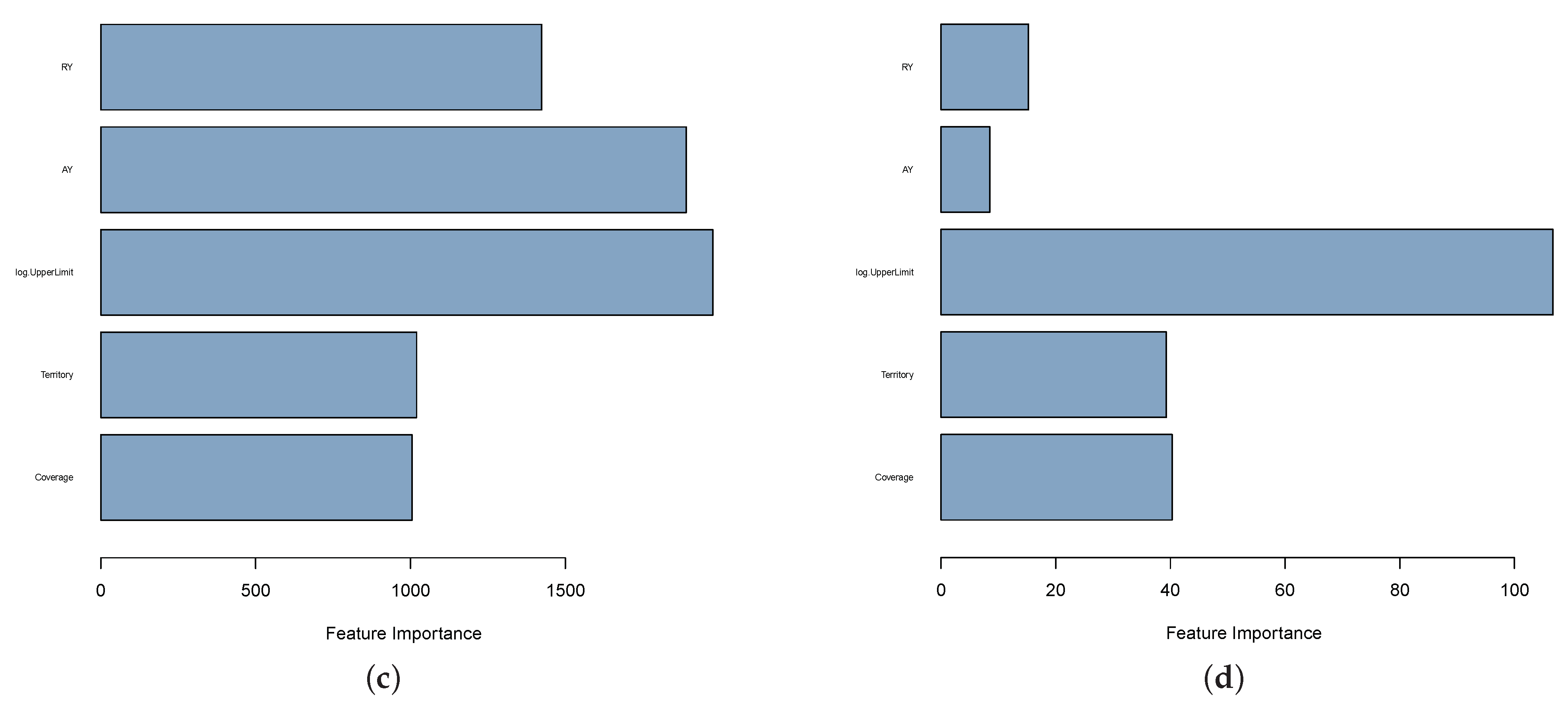
In the MLR model, given the fact that normality is assumed and the sampling distribution of model coefficients is also considered to be t distributed, the t values of the coefficients (i.e., coefficient estimate divided by its standard deviation) therefore become the importance measures of the independent variables. Similarly, in GLM, the variable importance measure can be the t value for each coefficient. However, there are some limitations of this approach. First of all, the biased estimate of the standard deviation of the coefficient may affect the results and significantly increase or decrease the measure of the variable importance. Secondly, the variable importance measures reflect the risk factor level rather than the risk factors themselves. Therefore, one has to further summarize the results from the importance measures of independent variables, which are associated with the risk factor level, so that the importance of risk factors can be quantified. One possible solution is to calculate the ratio of the average value of coefficients to its estimated standard deviation, which can be achieved by the following method.

Suppose that there are $k_i$ levels for the ith risk factor. We can then denote the model coefficient of the jth level of risk factor i to be ${\beta }_j^i$, and its standard deviation to be ${\sigma }_{{\beta }_j^i}$. We assume that ${\beta }_j^i>0$. If not, then we take the absolute value of the model coefficient to make it positive. We can further compute the average coefficients within the risk factor i, denoted by ${\overline{\beta }}^i=\frac{1}{k_i}{\sum }_{j=1}^{k_i}{\beta }_j^i$, and determine the standard deviation of such an average, denoted by $\frac{1}{k_i}\sqrt{{\sum }_{j=1}^{k_i}Var\left({\beta }_j^i\right)}$ or $\frac{1}{k_i}\sqrt{{\sum }_{j=1}^{k_i}{\sigma }_{{\beta }_j^i}^2}$, based on the independence assumption of coefficients. This leads to the following definition of the importance measure of the ith risk factor based on the ratio of average coefficients within the risk factor i and its estimated standard deviation, given as follows:

$$\begin{array}{c}\hfill VarIm{p}_i=\frac{{\sum }_{j=1}^{k_i}{\beta }_j^i}{\sqrt{{\sum }_{j=1}^{k_i}{\sigma }_{{\beta }_j^i}^2}}.\end{array}$$

(9)

In the case that normal distribution is used as a link function, $VarIm{p}_i$ given above becomes the variable importance measure for the ith factor in GLM.

In GLM modeling, in order to improve the stability of model variance, the response variable is often under a certain transformation, such as logarithmic transform. When this is the case, it is more suitable to measure the variance importance based on the original scale of variables. Therefore, the model coefficients need to be replaced by the inverse of the logarithmic, which is the exponential. As a result of this, Equation (9) becomes

$$\begin{array}{c}\hfill VarIm{p}_i=\frac{{\sum }_{j=1}^{k_i}{e}^{{\beta }_j^i}}{\sqrt{{\sum }_{j=1}^{k_i}Var\left(e^{{\beta }_j^i}\right)}},\end{array}$$

(10)

where $Var\left(e^{{\beta }_j^i}\right)$ can be approximated by taking the first-order Taylor series expansion of function $e^{{\beta }_j^i}$, and evaluated at ${\beta }_j^i=0$, which is given as follows:

$$\begin{array}{c}\hfill Var\left(e^{{\beta }_j^i}\right)\approx Var(1+{\beta }_j^i)=Var\left({\beta }_j^i\right)={\sigma }_{{\beta }_j^i}^2.\end{array}$$

(11)

Based on this result, we can obtain the variable importance measure for the case where logarithmic transform is applied to the response variable, which is the case corresponding to the Poisson error function. It is given as follows:

$$\begin{array}{c}\hfill VarIm{p}_i^{\left(P\right)}=\frac{{\sum }_{j=1}^{k_i}{e}^{{\beta }_j^i}}{\sqrt{{\sum }_{j=1}^{k_i}{\sigma }_{{\beta }_j^i}^2}}.\end{array}$$

(12)

This is applicable for both the multiple linear regression with the logarithmic transformation of the response variable, and the GLM with a logarithmic link function. For other cases, using the first-order Taylor series expansion for the mean function, we can evaluate the approximated variance of ${\sigma }_{{\beta }_j^i}^2$. Since all predictors are categorical, the scale change in ${\beta }_j$ to the original scale can be achieved simply by evaluating the mean function at $X_j=1$ for the given j, the level within risk factor i and zero for others. That is to say, we can use the following first order Taylor series expansion as an approximation if we denote $f\left({\beta }_j^i\right)$ as the mean function that is contributed by ${\beta }_j$ within factor i only, i.e.,

$$\begin{array}{c}\hfill f\left({\beta }_j^i\right)=f\left({\overline{\beta }}^i\right)+f^{\prime }\left({\overline{\beta }}^i\right)({\beta }_j^i-{\overline{\beta }}^i).\end{array}$$

(13)

Therefore, the variance of the mean function of ${\beta }_j^i$ becomes

$$\begin{array}{c}\hfill Var\left(f\left({\beta }_j^i\right)\right)\approx {\left(f^{\prime }\left({\overline{\beta }}^i\right)\right)}^{2}Var\left({\beta }_j^i\right).\end{array}$$

(14)

When the inverse Gaussian error function is used, we have the following variance importance for the ith factor:

$$\begin{array}{c}\hfill VarIm{p}_i^{\left(IG\right)}=\frac{2{\sum }_{j=1}^{k_i}{\left({\beta }_j^i\right)}^{-1/2}}{\sqrt{{\sum }_{j=1}^{k_i}\frac{1}{{\left({\overline{\beta }}^i\right)}^3}{\sigma }_{{\beta }_j^i}^2}}.\end{array}$$

(15)

Similarly, for the Gamma error function and the binomial error function, the variance importance measures are, respectively,

$$\begin{array}{c}\hfill VarIm{p}_i^{\left(G\right)}=\frac{{\sum }_{j=1}^{k_i}{\left({\beta }_j^i\right)}^{-1}}{\sqrt{{\sum }_{j=1}^{k_i}\frac{1}{{\overline{\beta }}^i}{\sigma }_{{\beta }_j^i}^2}},\mathrm{and}VarIm{p}_i^{\left(B\right)}=\frac{{\sum }_{j=1}^{k_i}\frac{e^{{\beta }_j^i}}{1+e^{{\beta }_j^i}}}{\sqrt{{\sum }_{j=1}^{k_i}\frac{e^{2{\overline{\beta }}^i}}{{(1+e^{{\overline{\beta }}^i})}^4}{\sigma }_{{\beta }_j^i}^2}}.\end{array}$$

(16)

In general, in the GLM setting, the variable importance measure for a given ith factor is defined as a ratio of the mean function evaluated at the ith factor and the square root of the approximated variance of the mean function, corresponding to the ith factor, which can be found in

Table 2. Summary of the results of variance approximation of average coefficients, and their corresponding link function and mean function in generalized linear models.

Error Distribution	Link Function	Mean Function	Variance Approximation
Normal	$X{\beta }^{\top }=\mu$	$\mu =X{\beta }^{\top }$	${\sum }_{j=1}^{k_i}{\sigma }_{{\beta }_j^i}^2$
Poisson	$X{\beta }^{\top }=ln\left(\mu \right)$	$\mu =exp\{X{\beta }^{\top }\}$	${\sum }_{j=1}^{k_i}{\sigma }_{{\beta }_j^i}^2$
Inverse Gaussian	$X{\beta }^{\top }={\mu }^{-2}$	$\mu ={\left(X{\beta }^{\top }\right)}^{-1/2}$	${\sum }_{j=1}^{k_i}\frac{1}{4{({\overline{\beta }}^i)}^3}{\sigma }_{{\beta }_j^i}^2$
Gamma	$X{\beta }^{\top }=-{\mu }^{-1}$	$\mu =-{\left(X{\beta }^{\top }\right)}^{-1}$	${\sum }_{j=1}^{k_i}\frac{1}{{\overline{\beta }}^i}{\sigma }_{{\beta }_j^i}^2$
Binomial	$X{\beta }^{\top }=ln(\frac{\mu }{1-\mu })$	$\mu =\frac{exp(X{\beta }^{\top })}{1+exp(X{\beta }^{\top })}$	${\sum }_{j=1}^{k_i}\frac{e^{2{\overline{\beta }}^i}}{{(1+e^{{\overline{\beta }}^i})}^4}{\sigma }_{{\beta }_j^i}^2$

for the cases that we consider. If there are only two levels for the given factor, the mean function is just the estimate of the coefficient for the non-base level. This implies that the variable importance measure for such a factor is just the t value associated with the given factor.

On the other hand, the proposed variable importance measures for GLM to capture the variable importance are based on the assumption that at least one of the estimated coefficients of factor levels is statistically significant. Suppose all coefficient estimates of all factor levels within the same factor are statistically insignificant. In that case, the variable importance measures may be impacted, particularly for the one associated with the gamma link function. If the link function is gamma and all coefficients of factor levels are close to zero, the variable importance measures will approach infinity. This can be seen from the following mathematical derivation.

In order to be able to discuss the convergence of the variable importance when ${\beta }_j$ approaches to zero, we first refer to the AM-HM inequality [28], which is given as follows:

$$\begin{array}{c}\hfill \frac{1}{n}\sum _{i=1}^n{x}_i\ge \frac{n}{{\sum }_{i=1}^n{x}_i^{-1}},\end{array}$$

(17)

for non-negative real values $x_i$. This implies that

$$\begin{array}{c}\hfill \sum _{i=1}^n{x}_i^{-1}\ge \frac{n^2}{{\sum }_{i=1}^n{x}_i}.\end{array}$$

(18)

Therefore, by applying the the AM-HM inequality to the $VarIm{p}_i^{\left(G\right)}$, we have

$$\frac{{\sum }_{j=1}^{k_i}{\left({\beta }_j^i\right)}^{-1}}{\sqrt{{\sum }_{j=1}^{k_i}\frac{1}{{\overline{\beta }}^i}{\sigma }_{{\beta }_j^i}^2}}\ge \frac{\frac{k_i^2}{{\sum }_{j=1}^{k_i}{\beta }_j^i}}{\sqrt{\frac{1}{{\overline{\beta }}^i}}·\sqrt{{\sum }_{j=1}^{k_i}{\sigma }_{{\beta }_j^i}^2}}$$

(19)

Let $\sqrt{{\sum }_{j=1}^{k_i}{\sigma }_{{\beta }_j^i}^2}=M$; then,

$$\frac{\frac{k_i^2}{{\sum }_{j=1}^{k_i}{\beta }_j^i}}{\sqrt{\frac{1}{{\overline{\beta }}^i}}·\sqrt{{\sum }_{j=1}^{k_i}{\sigma }_{{\beta }_j^i}^2}}=\frac{\frac{k_i}{{\overline{\beta }}^i}}{\sqrt{\frac{1}{{\overline{\beta }}^i}}M}=\frac{k_i}{\sqrt{{\overline{\beta }}^i}M}.$$

(20)

As ${\beta }_j\to 0$, for all j, ${\overline{\beta }}^i\to 0$, so ${lim}_{\overline{\beta }\to 0^{+}}\frac{k_i}{\sqrt{{\overline{\beta }}^i}M}=\infty$. When this is the case, the variable importance measure under the gamma link function for the ith factor will take only the largest value of the coefficient to the calculation.

4. Results

This section implements the results using different approaches to measuring the variable importance for model-based methods. We first conduct the sensitivity analysis using the Lek profile approach. Then, we consider an artificial neural network model with one layer and four hidden units within the layer, respectively, for claim counts and loss amounts. The neuralnet package in R was used to construct our neural network models, which are trained using backpropagation. The parameters are cross-validated within the function used in the package. This model is the best ANN model for the given data set and has been studied in [29]. Figure 1 shows the predicted values of the response variable by each risk factor while holding other risk factors constant. There are apparent patterns between groups. The results shown in Figure 1 and Figure 2 confirm part of previous findings in [29] with the addition of non-linear responses that vary by different data groupings, particularly for coverage and size-of-loss. Similarly, Figure 3 shows the result for the average loss per claim count as the response variable. There are almost the same patterns among groups, except for size-of-loss. In Figure 3, the pattern within groups for size-of-loss confirms the functionality between the average loss per claim count and the size-of-loss. The bar plots in Figure 2 and Figure 3 suggest that size-of-loss is the important variable for all groups and all cases, including claim counts, the claim amount and the average loss per claim count. This result is consistent with the results discussed previously using variable importance measures. However, this sensitivity did not directly indicate the variable importance using the quantitative measures. Instead, it qualitatively shows that the log.UpperLimit variable (the size of loss factor) is the most crucial variable.

In Figure 4 and Figure 5, decision-tree-based methods are used to produce variable importance measures. Using the XGBoosting method leads to a consistent ranking for the variables for both the claim amount and claim counts. The single decision tree ranks the size of the loss variable as the most important one, whereas the random forest suggests that the territory is the most important. The importance of the size of loss is not picked up by the random forest method. Due to the inconsistent results obtained from the decision-tree-based method, the difficulty of using the existing method was realized, and further investigation is needed to address this consistency. However, compared to the sensitivity analysis discussed above, the decision-tree-based method has been a better choice in practical predictive modeling as it uses quantitative measures for variables ranking. On the other hand, decision-tree-based models can handle the variable importance for each factor included in the model. The interpretability of the model in terms of variable importance is obtained, but how the tree-based models measure the variable importance is more difficult to understand; therefore, the model transparency is not high for this type of method, which is based on machine learning models.

In Figure 6 and Figure 7, the variable importance measure for each factor is displayed for different error functions in the GAM models. The selected error functions for GAM, including gamma and Poisson distributions, were considered for illustration purposes. It was observed that the GAM model leads to an overall consistent result for the variable importance for loss amounts and claim counts for the error functions that we consider. The obtained result reveals that the most important factor is the size of loss. This consistent result may serve as the benchmark. Another advantage of using GAM is the high transparency due to the linear and additive nature and how the variable importance measures are computed. However, the limitation of using GAM is that it becomes less justifiable when a categorical type of variable, coded by a numerical label (e.g., 1, 2, 3, …), is treated as functional. All of these three different but relevant methods indicate that the size of loss is the most important factor among all major risk factors that we consider.

In Figure 8, the variable importance measures based on the t value of the estimated coefficient of each factor level are displayed for the cases of using gamma and Poisson as the error distributions in GLM. The log scale loss amount and log scale claim counts are taken as the model response, respectively. It was observed that the results apply the measures to each factor level. Moreover, the t values of each level of the territory and coverage factors are much larger than other factor levels. This may suggest that the territory and coverage play a more critical role in modeling loss. When comparing the results obtained from other methods mentioned earlier, they are the inconsistency in terms of the variable importance. This may imply that if one uses the importance measures associated with factor levels in GLM, the results may be misleading, as all other relevant approaches reveal that the size of loss is the most important variable. However, from the result, one can see that the variable importance obtained using the loss amount is consistent with the result obtained from using claim counts.

In Figure 9 and Figure 10, the variable importance measures under different choices of link functions are displayed. Figure 9 shows the results for the model taking the log scale loss amount as the response variable, whereas Figure 10 reports the findings for the model taking log scale claim counts as the response variable. For both types of responses, all models lead to the same dominant factor: the size of loss. However, one can observe that the variable importance measures for the RY factor have been significantly inflated for the gamma link function case for both claim amount and claim counts. This can be understood by looking at results reported in

Table 3. GLM model output for gamma as the link function. In the second and third column, the first value represents the coefficient of the factor level and the value next to the coefficient estimate (which is the one with bracket) is the standard error of the estimated coefficient.

	Dependent Variable
	log.Loss	log.Counts
CoverageBI	0.008 *** (0.0005)	0.082 *** (0.003)
TerritoryU	−0.010 *** (0.0005)	−0.079 *** (0.003)
as.factor(Log.UpperLimit)1000	0.009 *** (0.002)	0.026 *** (0.009)
as.factor(Log.UpperLimit)2000	0.004 ** (0.002)	0.057 *** (0.010)
as.factor(Log.UpperLimit)3000	0.005 *** (0.002)	0.076 *** (0.010)
as.factor(Log.UpperLimit)4000	0.006 *** (0.002)	0.093 *** (0.010)
as.factor(Log.UpperLimit)5000	0.0004 (0.002)	0.078 *** (0.010)
as.factor(Log.UpperLimit)10,000	−0.012 *** (0.002)	0.032 *** (0.009)
as.factor(Log.UpperLimit)15,000	−0.012 *** (0.002)	0.049 *** (0.009)
as.factor(Log.UpperLimit)20,000	−0.013 *** (0.002)	0.060 *** (0.010)
as.factor(Log.UpperLimit)25,000	−0.013 *** (0.002)	0.071 *** (0.010)
as.factor(Log.UpperLimit)30,000	−0.015 *** (0.002)	0.068 *** (0.010)
as.factor(Log.UpperLimit)40,000	−0.020 *** (0.002)	0.045 *** (0.009)
as.factor(Log.UpperLimit)50,000	−0.019 *** (0.002)	0.063 *** (0.010)
as.factor(Log.UpperLimit)75,000	−0.024 *** (0.002)	0.043 *** (0.009)
as.factor(Log.UpperLimit)1 × 10${}^5$	−0.022 *** (0.002)	0.076 *** (0.010)
as.factor(Log.UpperLimit)150,000	−0.024 *** (0.002)	0.081 *** (0.010)
as.factor(Log.UpperLimit)2 × 10${}^5$	−0.020 *** (0.002)	0.134 *** (0.011)
as.factor(Log.UpperLimit)3 × 10${}^5$	−0.021 *** (0.002)	0.149 *** (0.011)
as.factor(Log.UpperLimit)4 × 10${}^5$	−0.019 *** (0.002)	0.218 *** (0.013)
as.factor(Log.UpperLimit)5 × 10${}^5$	−0.017 *** (0.002)	0.284 *** (0.014)
as.factor(Log.UpperLimit)750,000	−0.020 *** (0.002)	0.264 *** (0.014)
as.factor(Log.UpperLimit)1 × 10${}^6$	−0.018 *** (0.002)	0.365 *** (0.016)
as.factor(Log.UpperLimit)2 × 10${}^6$	−0.024 *** (0.002)	0.293 *** (0.014)
AY2010	−0.0005 (0.001)	−0.002 (0.007)
AY2011	0.001 (0.001)	0.011 (0.007)
AY2012	0.001 (0.001)	0.014 ** (0.007)
AY2013	0.0001 (0.001)	0.013 * (0.007)
AY2014	−0.0002 (0.001)	0.019 ** (0.009)
RY2014	−0.004 *** (0.001)	−0.034 *** (0.004)
Constant	0.151 *** (0.001)	0.304 *** (0.008)
Observations	960	920
Log Likelihood	−437.949	−346.747
Akaike Inf. Crit.	939.898	755.495

Note: * p < 0.1; ** p < 0.05; *** p < 0.01.

, where the insignificance of all levels of the RY factor is obtained for the loss amount. Some RY factor levels are either insignificant or less significant for the case when the claim count is used as the response variable. These may lead to the inflation of the variable importance measures as well. Note that the impact from the insignificance of factor level in the case of using the gamma link function has been explained in the previous section. One also observes that, when using the Gaussian and inverse Gaussian links function, the pattern of the variable importance measures is similar to the method of using GAM. This implies that the proposed method is more robust to the Gaussian or inverse Gaussian link functions, and, in practice, one may choose to use these two types of link functions whenever appropriate. On the other hand, the coefficients of factor levels for the size of loss are all statistically highly significant for both the claim amount and claim counts model. This may help to explain why the variable importance measures based on factors lead to the most dominant one being the size of loss, whereas the variable importance measures for factor levels in GLM miss that.

Overall, using our proposed method in GLM for evaluating the variable importance for the model factors, similar results with other existing methods were obtained. However, the significance of this work is that it was built on the merit of GLM in estimating the risk factor level, which provides the relativity measures of all of the risk factor levels involved. These results are needed in rate regulation, and they play an important role as a benchmark for rate filings review. Therefore, our approach is to improve GLM in rate-making by providing a suitable measure for model factors in terms of their importance.

5. Conclusions and Future Work

Interpretable machine learning models have played an important role in many real-world applications, including insurance pricing. Variable importance measures are key quantification techniques used to improve the model’s interpretability. In this work, a method that evaluates the importance of the model variables used in GLM was proposed to ensure that decision making based on factors becomes possible. This issue was illustrated by addressing the predictive modeling of the size of loss for regulation purposes. The variable importance for the major risk factor used in auto insurance rate regulation was investigated by applying various approaches. Our study reveals that the size of loss is the most dominant factor among all factors we consider. Our proposed method on variable importance measures exclusively for GLM modeling shows great success, and the ranking of variables in terms of their importance coincides with other methods. However, our method improves the GLM modeling by overcoming its difficulty in determining the factor importance rather than the importance of factor levels. This makes GLM modeling even wider for application to real-world predictive modeling due to this capability in capturing variable importance through our proposed method. Since GLM has been very popular in insurance pricing, it can now be further used for decision-making problems in risk management and the regulation of auto insurance. Our findings on variable importance measures of major risk factors can help insurance regulators to better understand the impact of risk factors on the model response when modeling loss amounts or claim loss. Therefore, better insights on insurance loss patterns are obtained.

Our method was proposed for variable importance measures of categorical variables in GLM. However, when it is numerical, the variable measure that we proposed for the numerical variable becomes just the t value, and there is only one estimate needed for each variable. This is the same thing as a categorical variable with only two levels. Therefore, the traditional ANOVA method or GAM model may also be appropriate in evaluating variable importance, but subject to its own limitation. Furthermore, since GLM has been widely used in insurance for risk modeling, further study of variable importance may help to deal with the variable selection or dimension reduction, therefore improving the statistical optimality of GLM modeling in real-world applications. Future work plans to extend the study of variable importance measures in GLM to other types of statistical plan data to further address the applicability of the proposed method in a broader area of insurance rate making.

References

1. David, M. Auto insurance premium calculation using generalized linear models. Procedia Econ. Financ. 2015, 20, 147–156. [Google Scholar] [CrossRef] [Green Version]
2. David, M.; Jemna, D.V. Modeling the frequency of auto insurance claims by means of poisson and negative binomial models. Analele Stiintifice ale Universitatii “Al. I. Cuza” din Iasi. Stiinte Economice/Scientific Annals of the “Al. I. Cuza” 2015, 62, 151–168. [Google Scholar] [CrossRef] [Green Version]
3. Ialongo, C. Understanding the effect size and its measures. Biochem. Med. 2016, 26, 150–163. [Google Scholar] [CrossRef] [Green Version]
4. Lee, D.K. Alternatives to P value: Confidence interval and effect size. Korean J. Anesthesiol. 2016, 69, 555. [Google Scholar] [CrossRef] [Green Version]
5. Heinze, G.; Wallisch, C.; Dunkler, D. Variable selection–a review and recommendations for the practicing statistician. Biom. J. 2018, 60, 431–449. [Google Scholar] [CrossRef] [Green Version]
6. Chun, H.; Keleş, S. Sparse partial least squares regression for simultaneous dimension reduction and variable selection. J. R. Stat. Soc. Ser. B (Stat. Methodol.) 2010, 72, 3–25. [Google Scholar] [CrossRef] [PubMed] [Green Version]
7. Ma, Y.; Zhu, L. A review on dimension reduction. Int. Stat. Rev. 2013, 81, 134–150. [Google Scholar] [CrossRef] [PubMed] [Green Version]
8. Strobl, C.; Boulesteix, A.L.; Kneib, T.; Augustin, T.; Zeileis, A. Conditional variable importance for random forests. BMC Bioinform. 2008, 9, 307. [Google Scholar] [CrossRef] [PubMed] [Green Version]
9. Thomas, D.R.; Zhu, P.; Zumbo, B.D.; Dutta, S. On measuring the relative importance of explanatory variables in a logistic regression. J. Mod. Appl. Stat. Methods 2008, 7, 4. [Google Scholar] [CrossRef] [Green Version]
10. Owen, A.B.; Prieur, C. On Shapley value for measuring importance of dependent inputs. SIAM/ASA J. Uncertain. Quantif. 2017, 5, 986–1002. [Google Scholar] [CrossRef] [Green Version]
11. Kuo, K.; Lupton, D. Towards explainability of machine learning models in insurance pricing. arXiv 2020, arXiv:2003.10674. [Google Scholar]
12. Murdoch, W.J.; Singh, C.; Kumbier, K.; Abbasi-Asl, R.; Yu, B. Interpretable machine learning: Definitions, methods, and applications. arXiv 2019, arXiv:1901.04592. [Google Scholar] [CrossRef] [Green Version]
13. Lorentzen, C.; Mayer, M. Peeking into the Black Box: An Actuarial Case Study for Interpretable Machine Learning. Available online: https://papers.ssrn.com/sol3/papers.cfm?abstract_id=3595944 (accessed on 1 March 2022).
14. Kościelniak, H.; Puto, A. BIG DATA in decision making processes of enterprises. Procedia Comput. Sci. 2015, 65, 1052–1058. [Google Scholar] [CrossRef] [Green Version]
15. Jeble, S.; Kumari, S.; Patil, Y. Role of big data in decision making. Oper. Supply Chain Manag. Int. J. 2017, 11, 36–44. [Google Scholar] [CrossRef] [Green Version]
16. Janssen, M.; van der Voort, H.; Wahyudi, A. Factors influencing big data decision-making quality. J. Bus. Res. 2017, 70, 338–345. [Google Scholar] [CrossRef]
17. Huang, Y.; Meng, S. Automobile insurance classification ratemaking based on telematics driving data. Decis. Support Syst. 2019, 127, 113156. [Google Scholar] [CrossRef]
18. Blier-Wong, C.; Cossette, H.; Lamontagne, L.; Marceau, E. Machine learning in P&C insurance: A review for pricing and reserving. Risks 2020, 9, 4. [Google Scholar]
19. Crevecoeur, J.; Antonio, K.; Desmedt, S.; Masquelein, A. Bridging the gap between pricing and reserving with an occurrence and development model for non-life insurance claims. arXiv 2022, arXiv:2203.07145. [Google Scholar]
20. Ohlsson, E.; Johansson, B. Non-Life Insurance Pricing with Generalized Linear Models; Springer: Berlin, Germany, 2010; Volume 174. [Google Scholar]
21. Branda, M. Optimization approaches to multiplicative tariff of rates estimation in non-life insurance. Asia-Pac. J. Oper. Res. 2014, 31, 1450032. [Google Scholar] [CrossRef] [Green Version]
22. Magri, A.; Farrugia, A.; Valletta, F.; Grima, S. An analysis of the risk factors determining motor insurance premium in a small island state: The case of Malta. Int. J. Financ. Insur. Risk Manag. 2019, 9, 63–85. [Google Scholar]
23. Gevrey, M.; Dimopoulos, I.; Lek, S. Review and comparison of methods to study the contribution of variables in artificial neural network models. Ecol. Model. 2003, 160, 249–264. [Google Scholar] [CrossRef]
24. Lek, S.; Delacoste, M.; Baran, P.; Dimopoulos, I.; Lauga, J.; Aulagnier, S. Application of neural networks to modelling nonlinear relationships in ecology. Ecol. Model. 1996, 90, 39–52. [Google Scholar] [CrossRef]
25. Breiman, L.; Friedman, J.H.; Olshen, R.A.; Stone, C.J. Classification and Regression Trees; Routledge: London, UK, 2017. [Google Scholar]
26. Hastie, T.; Tibshirani, R.; Friedman, J.H.; Friedman, J.H. The Elements of Statistical Learning: Data Mining, Inference, and Prediction; Springer: Berlin, Germany, 2009; Volume 2. [Google Scholar]
27. De Jong, P.; Heller, G.Z. Generalized Linear Models for Insurance Data; Cambridge Books; Cambridge University Press: Cambridge, UK, 2008. [Google Scholar]
28. Bencze, M. About AM-HM inequality. Octogon Math. Mag. 2009, 17, 106–116. [Google Scholar]
29. Xie, S. Improving explainability of major risk factors in artificial neural networks for auto insurance rate regulation. Risks 2021, 9, 126. [Google Scholar] [CrossRef]
Figure 1. Sensitivity analysis of ANN models using the Lek profile method to evaluate the effect of each risk factor. The figure sorts unevaluated risk factors into three groups. (a) Claim Counts. (b) Loss Amounts.
Mathematics 10 01630 g001
Figure 2. Bar plots for values of unevaluated risk factors in each group, where the value in each group is at the cluster mean. (a) Claim Counts. (b) Loss Amounts.
Mathematics 10 01630 g002
Figure 3. Bar plots for values of unevaluated risk factors in each group, where the group is at the cluster mean. (a) Claim Counts. (b) Loss Amounts.
Mathematics 10 01630 g003
Figure 4. Variable importance measured by tree-based methods using log scale loss amounts as model response variable.
Mathematics 10 01630 g004
Figure 5. Variable importance measured by tree-based methods using log scale claim counts as model response variable.
Mathematics 10 01630 g005
Figure 6. Bar plots for variable importance measures of risk factors in GAM based on the log scale claim amount. (a) Gamma as an error function in GAM. (b) Gaussian as an error function in GAM.
Mathematics 10 01630 g006
Figure 7. Bar plots for variable importance measures of risk factor in GAM based on the log scale claim counts. (The Poisson error function is with log link function). (a) Poisson as an error function in GAM. (b) Gaussian as an error function in GAM.
Mathematics 10 01630 g007
Figure 8. Bar plots for variable importance measure of each factor level in GLM based on the log scale claim amount. (a) Gamma as an error function in GLM, where Loss Amounts are used as the response variable. (b) Poisson as an error function in GLM, where Claim Counts are used as the response variable.
Mathematics 10 01630 g008
Figure 9. Bar plots for variable importance measures of risk factor in GLM based on the log scale loss amounts using our proposed method. (a) Poisson as an error function. (b) Gaussian as an error function. (c) Gamma as an error function. (d) Inverse Gaussian as an error function.
Mathematics 10 01630 g009
Figure 10. Bar plots for variable importance measures of risk factor in GLM based on the log scale claim counts using our proposed method. (The Poisson error function is with log link function). (a) Poisson as an error function. (b) Gaussian as an error function. (c) Gamma as an error function. (d) Inverse Gaussian as an error function.
Mathematics 10 01630 g010aMathematics 10 01630 g010b