Fuzzy-Based Adaptive Dynamic Surface Control for a Type of Uncertain Nonlinear System with Unknown Actuator Faults

Abstract

In this paper, the adaptive control problem of a type of uncertain nonlinear system is addressed. The system discussed includes unknown nonlinear functions, uncertain nonlinear dynamics, and unknown actuator faults. Based on the fuzzy logic systems and dynamic surface control technique, an adaptive fuzzy control law is designed to solve the tracking control problem. In control law design, fuzzy logic systems are utilized to approximate uncertain nonlinear functions, and with the help of the dynamic surface control technique, the problem of the “explosion of complexity” can be overcome. Through stability analysis, it is confirmed that all of the signals in the closed-loop system are semi-global bounded, and the convergence of the tracking error to the specified small neighborhood of the origin can be ensured by adjusting the control law parameters. Finally, the effectiveness of the proposed control law is verified by simulation examples.

1. Introduction

In the past decades, the adaptive control problems of nonlinear systems have received extensive attention in unmanned aerial vehicle systems, robotic systems, manipulator systems, and industrial control systems; see [1,2,3,4,5] and the references therein. To obtain better control performance, model predictive control [1], sliding mode control [4], state feedback control [6], and adaptive backstepping control [3,7] have been proposed. However, in several practical systems, there are usually complex nonlinear characteristics, such as uncertain nonlinear dynamics [2,8], strict-feedback nonlinear dynamics [7,9], nonaffine nonlinear dynamics [10], and pure-feedback nonlinear dynamics [11]. In the face of these complex nonlinear dynamics, how to design control laws and carry out the related theoretical analysis has always been a hot topic.

Due to the existence of nonlinear dynamics, some analysis approaches, such as the linearization method [12], the mean value theorem [13], the satisfaction of the Lipschitz condition [14], and the neural networks/fuzzy logic systems approximator [4,6,15,16,17] have been widely utilized. However, the methods considered in [12,13,14] usually need to meet some assumptions, such as the differentiable condition, the matching condition, or the growth condition, which are too strict for the analysis of practical nonlinear systems. Hence, the backstepping control technique is considered by some researchers for the control problem of nonlinear systems.

As an effective analytical method, the backstepping control technique is usually combined with various control methods to solve the control problems of various uncertain nonlinear systems. In [18,19], the adaptive backstepping control law was developed for the fractional-order nonlinear system and the strict-feedback nonlinear system, respectively. Owing to the application of design control laws, perfect tracking results can be achieved. In [20,21,22], the adaptive finite-time command filtered backstepping control law was designed to solve the tracking problem of uncertain nonlinear systems. In view of the approximation characteristics of neural networks and fuzzy logic systems, adaptive backstepping control approaches with neural networks or fuzzy logic systems are widely applied. In [23], the adaptive backstepping control schemes with fuzzy logic systems are proposed to solve the fault-tolerant control problem of nonlinear systems. In addition, by using the adaptive backstepping control law with neural networks, the tracking control problem of nonlinear systems with time-delay and unknown input saturation was achieved in [24], and the fault-tolerant control for a class of fractional-order nonlinear systems with actuator faults is discussed in [25].

In spite of the many control strategies with the backstepping control method that have been proposed and adopted in the existing literature, the problem of the “explosion of complexity” needs to be considered when using the backstepping control technique to design control laws. Given that virtual control laws and nonlinear functions need to be repeatedly differentiated in the backstepping recursive design, the complexity of the controller increases significantly with the increase of the order of the systems, especially for high-order nonlinear systems. For this purpose, the dynamic surface control approach has been considered by several researchers and does not require obtaining the derivative of virtual control laws in the previous step. Based on the advantage of the dynamic surface control method, the control problems of nonlinear systems with all kinds of constraints were designed in [26,27,28]. In [29,30], dynamic surface control laws with fuzzy logic systems were studied for the tracking problems of nonlinear systems with input saturation and time-varying output constraints and output delay, respectively. For the control problem of nonlinear large-scale systems with time delay, a better control effect was obtained by using the designed adaptive decentralized fuzzy dynamic surface control law in [31,32], and in [33,34], the dynamic surface control laws with neural networks for the control problems of interconnected systems and uncertain nonlinear systems were considered, respectively. Moreover, the neuro-fuzzy-based adaptive dynamic surface control strategy was investigated in [35].

In several practical systems, due to the influence and limitation of various factors, actuators may suffer from failure. For this, in [16,36], the adaptive fuzzy control laws for the nonlinear interconnected systems and stochastic nonlinear high-order multiagent systems were designed, where the coupled denial-of-service attacks and actuator faults and nonaffine nonlinear faults were considered. In [37], a set-invariance adaptive dynamic surface control scheme was designed for uncertain large-scale nonlinear input-saturated systems. Under the designed adaptive fuzzy tracking control scheme, the tracking problems of uncertain nonlinear systems with dead-zone input were analyzed in [9,10,38]. Moreover, the backlash failure [20], the stuck failure [39], and input quantization [40] were also considered by researchers. Nevertheless, it is worth noting that the occurrence of actuator faults is accidental, which makes the parameters of actuator faults unknown. Therefore, it is worth studying the control problems of systems with actuator faults.

Motivated by the above-mentioned research, this paper discusses the adaptive tracking control problem of a type of uncertain nonlinear system with unknown actuator faults. The main contributions of this paper are summarized as follows:

(1)

The adaptive fuzzy dynamic surface control scheme is designed for the uncertain nonlinear system in the presence of actuator faults, where the fault occurring in the system is assumed to be unknown. Compared with the references [41,42], the fault model considered in this paper is more general;

(2)

Different from references [18,19], the problem of the “explosion of complexity” can be overcome owing to the introduction of the dynamic surface control technique, and the derivation of nonlinear terms in the backstepping recursive design is eliminated. In addition, fuzzy logic systems are used to approximate the unknown nonlinear dynamics, which effectively reduces the difficulty of the control law design;

(3)

The effectiveness of the control law designed in this paper is proved by theoretical analysis. By adjusting the design parameters, it is also proved that all of the signals in the closed-loop system are semi-global bounded, and the tracking error converges to the specified small neighborhood of the origin.

The rest of this paper is organized as follows. In Section 2, the problem description and preliminaries are provided. In Section 3, the main results for the adaptive fuzzy dynamic surface control for the uncertain nonlinear system with unknown actuator faults are discussed. Thereafter, the stability analysis and simulation analysis are given in Section 4 and Section 5, respectively. Finally, the conclusions are briefly drawn in Section 6.

Notation 1.

Throughout this paper,$\left|\hspace{0.17em}\cdot \hspace{0.17em}\right|$denotes the absolute value of real number or the distance of real space$R$.${(\cdot )}^T$denotes the transposition of a vector.$\tan \mathrm{h}(\cdot )$denotes the hyperbolic tangent function.${\lambda }_{\max }(\mathit{X})$represents the largest eigenvalue of the matrix$\mathit{X}$.$H_{iM}$stands for the maximum value of function$H_i(\cdot )$. $\mathrm{diag}(\cdot )$is the diagonal matrix.${\overline{\mathit{x}}}_i(t)={\left[x_1(t),x_2(t),\dots ,x_i(t)\right]}^T$represents the states vector.$\widehat{\mathit{\theta }}$represents the estimation of the ideal parameter vector${\mathit{\theta }}^{*}$. ${\psi }_{id}$represents the$i\mathrm{th}$virtual control law.

2. Problem Description and Preliminaries

2.1. System Description

Consider a class of uncertain nonlinear system with unknown actuator faults as the following form:

$$\{\begin{array}{l}{\dot{x}}_i(t)=x_{i+1}(t)+f_i\left({\overline{\mathit{x}}}_i(t)\right),\hspace{0.17em}i=1,2,\dots ,n-1\\ {\dot{x}}_n(t)=\upsilon (t)+f_n\left({\overline{\mathit{x}}}_n(t)\right)+{\Delta }_n\left({\overline{\mathit{x}}}_n(t)\right)\\ y=x_1\end{array}$$

(1)

where ${\overline{\mathit{x}}}_i(t)={\left[x_1(t),x_2(t),\cdots ,x_i(t)\right]}^T$($i=1,2,\cdots ,n$), $x_1(t),\cdots ,x_n(t)$ and $\upsilon (t)$ represents the states of system and actual control input, respectively; $f_i\left({\overline{\mathit{x}}}_i(t)\right)$($i=1,2,\cdots ,n$) is an unknown smooth nonlinear function; ${\Delta }_n\left({\overline{\mathit{x}}}_n(t)\right)$ is an uncertain nonlinear dynamic.

In this paper, the model of the actuator fault is considered as the actuator’s loss of effectiveness and bias signal, which is described as:

$$\upsilon (t)=\rho u(t)+f_0(t),\hspace{0.17em}\forall t>t_1$$

(2)

where $\rho$ denotes the actuator health condition and satisfies $0<{\rho }_0\le \rho \le 1$, ${\rho }_0$ is an unknown positive constant; $u(t)$ is the control input to be designed; $f_0(t)$ denotes the bounded time-varying bias signal and occurs at any unknown instant $t_1$, then there exists an unknown positive constant $f_0^{*}$ and satisfies $\left|f_0(t)\right|\le f_0^{*}$, for $\forall t\ge t_1$. Clearly, $\rho =1$ indicates that the system is fault-free, and ${\rho }_0\le \rho <1$ indicates that the actuator’s partial loss of effort.

The control objective of this paper is to develop an adaptive control law $u(t)$ for the system (1) by combing the fuzzy logic systems and dynamic surface control technique such that the system output $y$ tracks the desired reference trajectory $y_d$ under the unknown actuator fault, and all of the signals in the closed-loop system are bounded.

Note 1: For practical complex systems, there are usually complex nonlinear dynamics, and their accurate mathematical model is often difficult to obtain. Thus, the smooth nonlinear functions $f_i\left({\overline{\mathit{x}}}_i(t)\right)$($i=1,2,\cdots ,n$) in system (1) are considered as the unknown nonlinear dynamics. In addition, in terms of possible external disturbances, unmolded dynamics, and modeling errors, they are uniformly considered and defined as the uncertain nonlinear dynamic ${\Delta }_n\left({\overline{\mathit{x}}}_n(t)\right)$ in system (1).

Note 2: For the fault model of the system, the main consideration in this paper is the actuator loss of effectiveness and bias signal. Based on the change of actuator health condition $\rho$ and time-varying bias signal $f_0(t)$, the fault types in different situations can be realized. Compared with these single fault types, such as input saturation fault [37], dead-zone input [10,38], the backlash failure [20], the stuck failure [39], and input quantization [40], the fault model considered in this paper is more general.

2.2. Fuzzy Logic Systems

A fuzzy logic system usually consists of four parts, that is, the fuzzifier, the fuzzy rule base, the fuzzy inference engine, and the defuzzifier [38]. The fuzzy rule base consists of the following of “if-then” rules:

$$R^l: \mathrm{If} x_1 \mathrm{is} F_1^l, \dots , \mathrm{and} x_n \mathrm{is} F_n^l,\mathrm{then}h \mathrm{is} G^l, l=1,2,\cdots ,M.$$

where $\mathit{x}={\left[x_1,x_2,\cdots ,x_n\right]}^T$ and $h$ are the fuzzy logic system’s input and output, respectively; $M$ is the number of “if-then” rules; $F_1^l,F_2^l,\cdots ,F_n^l$ and $G^l$ are fuzzy sets for linguistic variables $x_1,x_2,\cdots ,x_n$, and $h$, respectively.

According to the description in reference [38], the fuzzy logic system can be expressed as:

$$h(\mathit{x})=\frac{{\displaystyle {\sum }_{l=1}^M{\overline{h}}_l{\mathsf{\Pi }}_{i=1}^n{\mu }_{F_i^l}(x_i)}}{{\displaystyle {\sum }_{l=1}^M\left[{\mathsf{\Pi }}_{i=1}^n{\mu }_{F_i^l}(x_i)\right]}}$$

(3)

where ${\overline{h}}_l={\max }_{h\in R}{\mu }_{G^l}(h)$, ${\mu }_{F_i^l}(x_i)$ and ${\mu }_{G^l}(y)$ are membership functions of fuzzy sets $F_i^l$ and $G^l$, respectively.

Defining the fuzzy basis function as:

$${\xi }_l(\mathit{x})=\frac{{\mathsf{\Pi }}_{i=1}^n{\mu }_{F_i^l}(x_i)}{{\displaystyle {\sum }_{l=1}^M\left[{\mathsf{\Pi }}_{i=1}^n{\mu }_{F_i^l}(x_i)\right]}},\hspace{0.17em}l=1,2,\cdots ,M$$

(4)

Let ${\mathit{\theta }}^T=\left[{\overline{h}}_1,{\overline{h}}_2,\cdots ,{\overline{h}}_M\right]=\left[{\theta }_1,{\theta }_2,\cdots ,{\theta }_M\right]$ and $\mathit{\xi }(\mathit{x})={\left[{\xi }_1(\mathit{x}),{\xi }_2(\mathit{x}),\cdots ,{\xi }_M(\mathit{x})\right]}^T$, then (3) is rewritten as:

$$h(\mathit{x})={\mathit{\theta }}^T\mathit{\xi }(\mathit{x})$$

(5)

Lemma 1 [38].

For any continuous function$f(\mathit{x})$defined on a compact set${\mathsf{\Omega }}_{\mathit{x}}$and any given positive constant$\epsilon$, there exists a fuzzy logic system (5) such that:

$$\underset{\mathit{x}\in {\mathsf{\Omega }}_{\mathit{x}}}{\sup }\left|f(\mathit{x})-h(\mathit{x})\right|=\left|f(\mathit{x})-{\mathit{\theta }}^T\mathit{\xi }(\mathit{x})\right|\le \epsilon$$

(6)

where$\epsilon$is the approximation accuracy and can be arbitrarily small.

According to [10], let ${\mathit{\theta }}^{*}$ be the ideal parameter vector of the fuzzy logic system, then we have:

$${\mathit{\theta }}^{*}=\arg {\min }_{\mathit{\theta }\in {\mathsf{\Omega }}_{\mathit{\theta }}}\underset{\mathit{x}\in {\mathsf{\Omega }}_{\mathit{x}}}{\sup }\left|f(\mathit{x})-{\mathit{\theta }}^T\mathit{\xi }(\mathit{x})\right|$$

(7)

where ${\mathsf{\Omega }}_{\mathit{\theta }}$ and ${\mathsf{\Omega }}_{\mathit{x}}$ are the compact set for $\mathit{\theta }$ and $\mathit{x}$.

Note 3: According to Lemma 1, the fuzzy logic systems can uniformly approximate a real continuous nonlinear function $f(\mathit{x})$ on the compact set $\mathsf{\Omega }$. Hence, there exists an ideal parameter vector ${\mathit{\theta }}^{*}$ and the approximation error $\epsilon$, which satisfy $f(\mathit{x})={\mathit{\theta }}^{*T}\mathit{\xi }(\mathit{x})+\epsilon$ with $\left|\epsilon \right|\le {\epsilon }^{*}$, $\forall \mathit{x}\in \mathsf{\Omega }$, where ${\epsilon }^{*}$ is an unknown positive constant. It should be noted that the ideal parameter vector ${\mathit{\theta }}^{*}$ is only utilized for analytical purposes and that the estimate parameter vector $\widehat{\mathit{\theta }}$ is utilized for control law design.

2.3. Preliminaries

Throughout this paper, the following assumptions and lemmas are used to analyze the main results.

Assumption 1.

The uncertain nonlinear dynamic${\Delta }_n\left({\overline{\mathit{x}}}_n(t)\right)$in system (1) is bounded, and there exists$\left|{\Delta }_n\left({\overline{\mathit{x}}}_n(t)\right)\right|\le {\Delta }_n^{*}$with${\Delta }_n^{*}$being a positive constant.

Assumption 2.

The desired reference trajectory$y_d$is bounded, and its first-, second-order derivatives exist and belong to compact set${\mathsf{\Xi }}_1$. Then there exists a positive constant$K_0$such that${\mathsf{\Xi }}_1:\left\{(y_d,{\dot{y}}_d,{\ddot{y}}_d):y_d^2+{\dot{y}}_d^2+{\ddot{y}}_d^2\le K_0\right\}$.

Lemma 2 [15].

For any$b\in R$and$\vartheta >0$, the hyperbolic tangent function$\tanh (\cdot )$satisfies:

$$\{\begin{array}{l}0\le \left|b\right|-b\tanh (\frac{b}{\vartheta })\le 0.2785\vartheta \\ 0\le b\tanh (\frac{b}{\vartheta })\end{array}$$

(8)

Lemma 3 [15].

For any variables$x\in R$and$y\in R$, the following inequality holds:

$$xy\le \frac{{\nu }^p}{p}{\left|x\right|}^p+\frac{1}{q{\nu }^q}{\left|y\right|}^q$$

(9)

where$\nu >0$,$p>1$,$q>1$and$(p-1)(q-1)=1$.

Note 4: For Assumption 1, it is the stability condition of the controllability $n$ order nonlinear system (1), which can ensure the design of the subsequent virtual control laws and the final control law. It should be noted that the boundedness of ${\Delta }_n\left({\overline{\mathit{x}}}_n(t)\right)$ is considered for the purpose of theoretical analysis. For Assumption 2, it is a common and fairly standard condition for the adaptive tracking control under the dynamic surface control design framework and can be seen in [8,9,13].

For the convenience of discussion in the next section, the time variable $t$ will be ignored without causing confusion.

3. Adaptive Fuzzy Dynamic Surface Controller Design

In this section, the fuzzy logic systems are introduced to approximate the unknown smooth nonlinear function, and then an adaptive fuzzy control scheme with dynamic surface control technique is addressed. The control law design is based on the following change of coordinates:

$$\{\begin{array}{l}{S}_1=e_1=x_1-y_d\\ S_i=x_i-y_{id},\hspace{0.17em}i=2,3,\cdots ,n\end{array}$$

(10)

where $e_1$ is the tracking error and $y_{id}$ is the output of a given first-order filter with the virtual control law ${\psi }_{id}$ as the input; $S_1,S_2,\cdots ,S_n$ are the defined sliding mode switching functions.

The design procedure involves $n$ steps. In step $i-1$($i=2,\cdots ,n$), the virtual control law ${\psi }_{id}$ is proposed to make the corresponding subsystem toward the equilibrium position, and in step $n$, the actual control law $u(t)$ will be developed.

Step 1. Considering the subsystem ${\dot{x}}_1=x_2+f_1({\overline{\mathit{x}}}_1)$ and noting (10), the derivative of $S_1$ is obtained as:

$${\dot{S}}_1=x_2+f_1({\overline{\mathit{x}}}_1)-{\dot{y}}_d$$

(11)

According to Lemma 1, the first fuzzy logic system is utilized to approximate the unknown smooth nonlinear function $f_1({\overline{\mathit{x}}}_1)$ as follows:

$$f_1({\overline{\mathit{x}}}_1)={({\mathit{\theta }}_1^{*})}^T{\mathit{\xi }}_1({\overline{\mathit{x}}}_1)+{\epsilon }_1({\overline{\mathit{x}}}_1)$$

(12)

where $\left|{\epsilon }_1({\overline{\mathit{x}}}_1)\right|\le {\epsilon }_1^{*}$ with ${\epsilon }_1^{*}$ being a positive constant.

Choosing $V(S_1)=S_1^2/2$ and differentiating $V(S_1)$ along (11) gives:

$$\dot{V}(S_1)=S_1{x}_2+S_1{f}_1({\overline{\mathit{x}}}_1)-S_1{\dot{y}}_d$$

(13)

Substituting (12) into (13) results in:

$$\dot{V}(S_1)\le S_1{x}_2+S_1{({\mathit{\theta }}_1^{*})}^T{\mathit{\xi }}_1({\overline{\mathit{x}}}_1)+\left|S_1\right|{\epsilon }_1^{*}-S_1{\dot{y}}_d$$

(14)

By virtue of (14), the virtual control law ${\psi }_{2d}$ and the adaptation law ${\dot{\widehat{\mathit{\theta }}}}_1$ are hence designed as:

$${\psi }_{2d}=-{({\widehat{\mathit{\theta }}}_1)}^T{\mathit{\xi }}_1({\overline{\mathit{x}}}_1)-{\epsilon }_1^{*}\tanh (\frac{{\epsilon }_1^{*}{S}_1}{\vartheta })-c_1{S}_1+{\dot{y}}_d$$

(15)

$${\dot{\widehat{\mathit{\theta }}}}_1={\mathbf{\Phi }}_1{\mathit{\xi }}_1({\overline{\mathit{x}}}_1)S_1-{\eta }_1{\mathbf{\Phi }}_1({\widehat{\mathit{\theta }}}_1-{\widehat{\mathit{\theta }}}_1^0)$$

(16)

where $c_1>0$ and ${\eta }_1>0$ are the designed parameters; ${\mathbf{\Phi }}_1$ is the positive definite symmetric matrix to be designed; ${\widehat{\mathit{\theta }}}_1$ is the estimate of ideal parameter vector ${\mathit{\theta }}_1^{*}$ of the first fuzzy logic system; and ${\widehat{\mathit{\theta }}}_1^0$ is the initial parameter vector.

In order to avoid differentiating the virtual control law ${\psi }_{2d}$ in the next step, the first-order filter with time constant ${\tau }_2$ is introduced to filter the control law ${\psi }_{2d}$ and then we have:

$${\tau }_2{\dot{y}}_{2d}+y_{2d}={\psi }_{2d},\hspace{0.17em}{\psi }_{2d}(0)=y_{2d}(0)$$

(17)

where $y_{2d}$ is the output of the first-order filter, ${\psi }_{2d}(0)$ which is given an initial value.

Furthermore, defining the filter error of the first-order filter as $z_2=y_{2d}-{\psi }_{2d}$, it is obtained from (17) that ${\dot{y}}_{2d}=-\left(z_2/{\tau }_2\right)$. Thus, taking the derivative of $z_2$ gives:

$$\begin{array}{l}{\dot{z}}_2=-\frac{z_2}{{\tau }_2}-\left(\frac{\partial {\psi }_{2d}}{\partial {\widehat{\mathit{\theta }}}_1}{\dot{\widehat{\mathit{\theta }}}}_1+\frac{\partial {\psi }_{2d}}{\partial {\overline{\mathit{x}}}_1}{\dot{\overline{\mathit{x}}}}_1+\frac{\partial {\psi }_{2d}}{\partial S_1}{\dot{S}}_1-\frac{\partial {\psi }_{2d}}{\partial {\dot{y}}_d}{\ddot{y}}_d\right)\\ \hspace{1em}=-\frac{z_2}{{\tau }_2}+H_2\left(S_1,S_2,z_2,{\widehat{\mathit{\theta }}}_1,y_d,{\dot{y}}_d,{\ddot{y}}_d\right)\end{array}$$

(18)

where $H_2(\cdot )$ is the introduced nonnegative continuous function, and it is to be applied for the stability analysis in the next section.

Choosing $V(z_2)=z_2^2/2$, and using Lemma 3, differentiating $V(z_2)$ along (18) yields:

$$\dot{V}(z_2)\le -\frac{z_{{}_2}^2}{{\tau }_2}+\left|z_2\right|H_2\le -\left(\frac{1}{{\tau }_2}-\frac{1}{2}\right)z_2^2+\frac{H_2^2}{2}$$

(19)

In addition, note that $x_2=S_2+y_{2d}$ and $z_2=y_{2d}-{\psi }_{2d}$, and then:

$$x_2=S_2+z_2+{\psi }_{2d}$$

(20)

According to Lemma 2, substituting (15) and (20) into (14) obtains:

$$\dot{V}(S_1)\le -c_1{S}_1^2+S_1{S}_2+S_1{z}_2-S_1{({\tilde{\mathit{\theta }}}_1)}^T{\mathit{\xi }}_1({\overline{\mathit{x}}}_1)+0.2785\vartheta$$

(21)

where ${\tilde{\mathit{\theta }}}_1={\widehat{\mathit{\theta }}}_1-{\mathit{\theta }}_1^{*}$, ${\tilde{\mathit{\theta }}}_1$ represents the estimation error.

Designing the following Lyapunov function candidate:

$$V_1=V(S_1)+V(z_2)+\frac{1}{2}{({\tilde{\mathit{\theta }}}_1)}^T{\mathbf{\Phi }}_1^{-1}{\tilde{\mathit{\theta }}}_1$$

(22)

Taking the time derivative of $V_1$ and substituting (19) and (21), we obtain:

$${\dot{V}}_1\le -c_1{S}_1^2+S_1{S}_2+S_1{z}_2-\left(\frac{1}{{\tau }_2}-\frac{1}{2}\right)z_2^2-S_1{({\tilde{\mathit{\theta }}}_1)}^T{\mathit{\xi }}_1({\overline{\mathit{x}}}_1)+{({\tilde{\mathit{\theta }}}_1)}^T{\mathbf{\Phi }}_1^{-1}{\dot{\tilde{\mathit{\theta }}}}_1+\frac{H_2^2}{2}+0.2785\vartheta$$

(23)

By virtue of ${\dot{\tilde{\mathit{\theta }}}}_1={\dot{\widehat{\mathit{\theta }}}}_1$ and Lemma 3, we obtain:

$${({\tilde{\mathit{\theta }}}_1)}^T({\widehat{\mathit{\theta }}}_1-{\widehat{\mathit{\theta }}}_1^0)={({\tilde{\mathit{\theta }}}_1)}^T({\tilde{\mathit{\theta }}}_1+{\mathit{\theta }}_1^{*}-{\widehat{\mathit{\theta }}}_1^0)\ge \frac{1}{2}{({\tilde{\mathit{\theta }}}_1)}^T({\tilde{\mathit{\theta }}}_1)-\frac{1}{2}{({\mathit{\theta }}_1^{*}-{\widehat{\mathit{\theta }}}_1^0)}^T({\mathit{\theta }}_1^{*}-{\widehat{\mathit{\theta }}}_1^0)$$

(24)

Then, substituting (16) and (24) into (23) becomes:

$$\begin{array}{l}{\dot{V}}_1\le -c_1{S}_1^2-\left(\frac{1}{{\tau }_2}-\frac{1}{2}\right)z_2^2-\frac{{\eta }_1}{2}{({\tilde{\mathit{\theta }}}_1)}^T({\tilde{\mathit{\theta }}}_1)+S_1{S}_2+S_1{z}_2+\frac{H_2^2}{2}\\ \hspace{1em}\hspace{0.17em}\hspace{0.17em}+\frac{{\eta }_1}{2}{({\mathit{\theta }}_1^{*}-{\widehat{\mathit{\theta }}}_1^0)}^T({\mathit{\theta }}_1^{*}-{\widehat{\mathit{\theta }}}_1^0)+0.2785\vartheta \end{array}$$

(25)

Step$i$ ($2\le i\le n-1$). Considering the subsystem ${\dot{x}}_i=x_{i+1}+f_i({\overline{\mathit{x}}}_i)$ and noting (10), the derivative of $S_i$ is obtained as:

$${\dot{S}}_i=x_i+f_i({\overline{\mathit{x}}}_i)-{\dot{y}}_{id}$$

(26)

The $i\mathrm{th}$ fuzzy logic system is used to approximate the unknown smooth nonlinear function $f_i({\overline{\mathit{x}}}_i)$ as follows:

$$f_i({\overline{\mathit{x}}}_i)={({\mathit{\theta }}_i^{*})}^T{\mathit{\xi }}_i({\overline{\mathit{x}}}_i)+{\epsilon }_i({\overline{\mathit{x}}}_i)$$

(27)

where $\left|{\epsilon }_i({\overline{\mathit{x}}}_i)\right|\le {\epsilon }_i^{*}$ with ${\epsilon }_i^{*}$ as a positive constant.

Similarly, considering $V(S_i)=S_i^2/2$ and differentiating $V(S_i)$ along (26) gives:

$$\dot{V}(S_i)\le S_i{x}_{i+1}+S_i\left({({\mathit{\theta }}_i^{*})}^T{\mathit{\xi }}_i({\overline{\mathit{x}}}_i)-{\dot{y}}_{id}\right)+\left|S_i\right|{\epsilon }_i^{*}$$

(28)

Designing the virtual control law ${\psi }_{(i+1)d}$ and the adaptation law ${\dot{\widehat{\mathit{\theta }}}}_i$ as follows:

$${\psi }_{(i+1)d}=-{({\widehat{\mathit{\theta }}}_i)}^T{\mathit{\xi }}_i({\overline{\mathit{x}}}_i)-{\epsilon }_i^{*}\tanh (\frac{{\epsilon }_i^{*}{S}_i}{\vartheta })-c_i{S}_i-S_{i-1}+{\dot{y}}_{id}$$

(29)

$${\dot{\widehat{\mathit{\theta }}}}_i={\mathbf{\Phi }}_i{\mathit{\xi }}_i({\overline{\mathit{x}}}_i)S_i-{\eta }_i{\mathbf{\Phi }}_i({\widehat{\mathit{\theta }}}_i-{\widehat{\mathit{\theta }}}_i^0)$$

(30)

where $c_i>0$ and ${\eta }_i>0$ are the designed parameters, ${\mathbf{\Phi }}_i$ is the positive definite symmetric matrix to be designed, ${\widehat{\mathit{\theta }}}_i$ is the estimate of the ideal parameter vector ${\mathit{\theta }}_i^{*}$ of the $i\mathrm{th}$ fuzzy logic system, and ${\widehat{\mathit{\theta }}}_i^0$ is the initial parameter vector.

Let ${\psi }_{(i+1)d}$ pass through the first-order filter with time constant ${\tau }_{i+1}$, and then we obtain $y_{(i+1)d}$ as:

$${\tau }_{i+1}{\dot{y}}_{(i+1)d}+y_{(i+1)d}={\psi }_{(i+1)d},\hspace{0.17em}{\psi }_{(i+1)d}(0)=y_{(i+1)d}(0)$$

(31)

where $y_{(i+1)d}$ is the output of first-order filter, ${\psi }_{(i+1)d}(0)$ is given an initial value.

Defining the filter error of the first-order filter as $z_{i+1}=y_{(i+1)d}-{\psi }_{(i+1)d}$ and considering ${\dot{y}}_{(i+1)d}=-\left(z_{i+1}/{\tau }_{i+1}\right)$, we obtain:

$$\begin{array}{l}{\dot{z}}_{i+1}=-\frac{z_{i+1}}{{\tau }_{i+1}}-\left(\frac{\partial {\psi }_{(i+1)d}}{\partial {\widehat{\mathit{\theta }}}_i}{\dot{\widehat{\mathit{\theta }}}}_i+\frac{\partial {\psi }_{(i+1)d}}{\partial {\overline{\mathit{x}}}_i}{\dot{\overline{\mathit{x}}}}_i+\frac{\partial {\psi }_{(i+1)d}}{\partial S_i}{\dot{S}}_i-\frac{\partial {\psi }_{(i+1)d}}{\partial {\dot{y}}_{(i+1)d}}{\ddot{y}}_{(i+1)d}\right)\\ \hspace{1em}\hspace{0.17em}=-\frac{z_{i+1}}{{\tau }_{i+1}}+H_{i+1}\left(S_1,S_2,\cdots ,S_{i+1},z_2,z_3,\cdots ,z_{i+1},{\widehat{\mathit{\theta }}}_1,{\widehat{\mathit{\theta }}}_2,\cdots ,{\widehat{\mathit{\theta }}}_i,y_d,{\dot{y}}_d,{\ddot{y}}_d\right)\end{array}$$

(32)

where $H_{i+1}(\cdot )$ is the introduced nonnegative continuous function.

Correspondingly, choosing $V(z_{i+1})=z_{i+1}^2/2$ and using Lemma 3, differentiating $V(z_{i+1})$ along (32) yields:

$$\dot{V}(z_{i+1})\le -\left(\frac{1}{{\tau }_{i+1}}-\frac{1}{2}\right)z_{{}_{i+1}}^2+\frac{H_{i+1}^2}{2}$$

(33)

Furthermore, considering $x_{i+1}=S_{i+1}+z_{i+1}+{\psi }_{(i+1)d}$ and (29), (28) can be rewritten as:

$$\dot{V}(S_i)\le -c_i{S}_i^2-S_{i-1}{S}_i+S_i{S}_{i+1}+S_i{z}_{i+1}-S_i{({\tilde{\mathit{\theta }}}_i)}^T{\mathit{\xi }}_i({\overline{\mathit{x}}}_i)+0.2785\vartheta$$

(34)

Designing the Lyapunov function $V_i$ as follows:

$$V_i=V(S_i)+V(Z_{i+1})+\frac{1}{2}{({\tilde{\mathit{\theta }}}_i)}^T{\mathbf{\Phi }}_1^{-1}{\tilde{\mathit{\theta }}}_i$$

(35)

where ${\tilde{\mathit{\theta }}}_i={\widehat{\mathit{\theta }}}_i-{\mathit{\theta }}_i^{*}$, and ${\tilde{\mathit{\theta }}}_i$ represents the estimation error.

Thus, according to (30), (33), (34), and Lemma 3, we obtain:

$$\begin{array}{l}{\dot{V}}_i\le -c_i{S}_i^2-\left(\frac{1}{{\tau }_{i+1}}-\frac{1}{2}\right)z_{{}_{i+1}}^2-\frac{{\eta }_i}{2}{({\tilde{\mathit{\theta }}}_i)}^T({\tilde{\mathit{\theta }}}_i)-S_{i-1}{S}_i+S_i{S}_{i+1}+S_i{z}_{i+1}+\frac{H_{i+1}^2}{2}+0.2785\vartheta \\ \hspace{1em}\hspace{0.17em}\hspace{0.17em}+\frac{{\eta }_i}{2}{({\mathit{\theta }}_i^{*}-{\widehat{\mathit{\theta }}}_i^0)}^T({\mathit{\theta }}_i^{*}-{\widehat{\mathit{\theta }}}_i^0)\end{array}$$

(36)

Step$n$. This is the last step. Considering the subsystem ${\dot{x}}_n(t)=\upsilon (t)+f_n({\overline{\mathit{x}}}_n)+{\Delta }_n({\overline{\mathit{x}}}_n)$ and noting (2) and (10), we obtain:

$${\dot{S}}_n=\rho u(t)+f_0(t)+f_n({\overline{\mathit{x}}}_n)+{\Delta }_n({\overline{\mathit{x}}}_n)-{\dot{y}}_{nd}$$

(37)

Considering the $n\mathrm{th}$ fuzzy logic system, then we obtain:

$$f_n({\overline{\mathit{x}}}_n)={({\mathit{\theta }}_n^{*})}^T{\mathit{\xi }}_n({\overline{\mathit{x}}}_n)+{\epsilon }_n({\overline{\mathit{x}}}_n)$$

(38)

where $\left|{\epsilon }_n({\overline{\mathit{x}}}_n)\right|\le {\epsilon }_n^{*}$ with ${\epsilon }_n^{*}$ as a positive constant.

Similarly, choosing $V(S_n)=S_n^2/2$, and considering (37) and (38), it is obtained that:

$$\dot{V}(S_n)\le S_n\left(\rho u(t)+{({\mathit{\theta }}_n^{*})}^T{\mathit{\xi }}_n({\overline{\mathit{x}}}_n)-{\dot{y}}_{nd}\right)+\left|S_n\right|{\mu }_n^{*}$$

(39)

where ${\mu }_n^{*}=f_0^{*}+{\epsilon }_n^{*}+{\Delta }_n^{*}$.

Taking,

$${\alpha }_n(t)={({\widehat{\mathit{\theta }}}_n)}^T{\mathit{\xi }}_n({\overline{\mathit{x}}}_n)+{\mu }_n^{*}\tanh (\frac{{\mu }_n^{*}{S}_n}{\vartheta })+c_n{S}_n+S_{n-1}-{\dot{y}}_{nd}$$

(40)

where $c_n>0$ is the designed parameter.

Due to $\rho$ being an unknown constant, let ${\delta }_n=1/\rho$ and ${\widehat{\delta }}_n$ be the estimate of ${\delta }_n$, then the following control law $u(t)$ and adaptation laws ${\widehat{\mathit{\theta }}}_n$ and ${\widehat{\delta }}_n$ are designed as:

$$u(t)=-{\widehat{\delta }}_n{\alpha }_n(t)$$

(41)

$${\dot{\widehat{\mathit{\theta }}}}_n={\mathbf{\Phi }}_n{\mathit{\xi }}_n({\overline{\mathit{x}}}_n)S_n-{\eta }_n{\mathbf{\Phi }}_n({\widehat{\mathit{\theta }}}_n-{\widehat{\mathit{\theta }}}_n^0)$$

(42)

$${\dot{\widehat{\delta }}}_n=S_n{\alpha }_n(t)-{\pi }_n{\widehat{\delta }}_n$$

(43)

where ${\eta }_n>0$ and ${\pi }_n>0$ are the designed parameters; ${\mathbf{\Phi }}_n$ is the positive definite symmetric matrix to be designed; ${\widehat{\mathit{\theta }}}_n$ is the estimate of ideal parameter vector ${\mathit{\theta }}_n^{*}$ of the $n\mathrm{th}$ fuzzy logic system and ${\widehat{\mathit{\theta }}}_n^0$ is the initial parameter vector.

Choosing the Lyapunov function $V_n$ as:

$$V_n=V(S_n)+\frac{1}{2}{({\tilde{\mathit{\theta }}}_n)}^T{\mathbf{\Phi }}_n^{-1}{\tilde{\mathit{\theta }}}_n$$

(44)

where ${\tilde{\mathit{\theta }}}_n={\widehat{\mathit{\theta }}}_n-{\mathit{\theta }}_n^{*}$, and ${\tilde{\mathit{\theta }}}_n$ represents the estimation error.

Similarly, following the same way of step $i$ and considering (41) and (42), we obtain:

$${\dot{V}}_n\le S_n({\alpha }_n-\rho {\widehat{\delta }}_n{\alpha }_n)-c_n{S}_n^2-\frac{{\eta }_n}{2}{({\tilde{\mathit{\theta }}}_n)}^T({\tilde{\mathit{\theta }}}_n)-S_{n-1}{S}_n+\frac{{\eta }_n}{2}{({\mathit{\theta }}_n^{*}-{\widehat{\mathit{\theta }}}_n^0)}^T({\mathit{\theta }}_n^{*}-{\widehat{\mathit{\theta }}}_n^0)+0.2785\vartheta$$

(45)

So far, the design process of the adaptive fuzzy dynamic surface controller has been completed.

Note 5: In this paper, the adaptive fuzzy dynamic surface control law is applied for the uncertain nonlinear systems with actuator faults. Based on the application of dynamic surface control technology, the derivation of nonlinear terms in the design of virtual control laws and the final actual control law is avoided. In addition, we also found that in some studies, such as references [20,21,22], the command filter control method is introduced to improve the traditional backstepping control method. It is found that the implementation of the command filter control method needs to introduce a compensation signal and then construct the compensation signal error. Hence, by comparison, the implementation of the dynamic surface control method is more intuitive and only needs to design a kind of first-order low-pass filter. Then, the design of the virtual control law and final actual control law can be well simplified. However, the command filter also has its own advantages, which can still well avoid the explosion of complexity problems in the design of virtual control laws and adaptive updating laws.

4. Stability Analysis

In this section, the stability analysis is elaborated and it is proved that all of the signals in the closed-loop system are semi-global bounded.

Theorem 1.

Considering the uncertain nonlinear system with actuator fault (1) under the Assumptions 1 and 2, the virtual control laws are designed as (15) and (29) with the adaptation laws constructed as (16) and (30), and the control law is designed as (41) with (40) and the adaptation laws constructed as (42) and (43), then there exist$c_i$,${\eta }_i$,${\mathbf{\Phi }}_i$($i=1,2,\cdots ,n$),${\tau }_i$($i=2,\cdots ,n$),${\pi }_n$and$\vartheta$such that all of the signals in the closed-loop system are semi-global bounded and the tracking error can be guaranteed to converge to the specified small neighborhood of the origin by adjusting the control law parameters.

Proof: 

Consider the Lyapunov function as follows:

$$V={\displaystyle \sum _{i=1}^n{V}_i}+\frac{\rho }{2}{\tilde{\delta }}_n^2$$

(46)

where ${\tilde{\delta }}_n={\widehat{\delta }}_n-{\delta }_n$, and ${\tilde{\delta }}_n$ represents the estimation error.

It follows from (25), (36), and (45) that the time derivative of $V$ yields:

$$\begin{array}{l}\dot{V}\le S_n({\alpha }_n-\rho {\widehat{\delta }}_n{\alpha }_n)-{\displaystyle \sum _{i=1}^n{c}_i{S}_i^2}-{\displaystyle \sum _{i=2}^n(\frac{1}{{\tau }_i}-\frac{1}{2})z_{{}_i}^2}-{\displaystyle \sum _{i=1}^n\frac{{\eta }_i}{2}{({\tilde{\mathit{\theta }}}_i)}^T({\tilde{\mathit{\theta }}}_i)}+{\displaystyle \sum _{i=1}^{n-1}{S}_i{z}_{i+1}}+\rho {\tilde{\delta }}_n{\dot{\tilde{\delta }}}_n\\ \hspace{1em}\hspace{0.17em}\hspace{0.17em}+{\displaystyle \sum _{i=1}^n\frac{{\eta }_i{({\mathit{\theta }}_i^{*}-{\widehat{\mathit{\theta }}}_i^0)}^T({\mathit{\theta }}_i^{*}-{\widehat{\mathit{\theta }}}_i^0)}{2}}+{\displaystyle \sum _{i=1}^n\frac{H_i^2}{2}}+0.2785n\vartheta \end{array}$$

(47)

Based on Lemma 3, we obtain:

$$S_i{z}_{i+1}\le \frac{S_i^2}{2}+\frac{z_{i+1}^2}{2}$$

(48)

$${\tilde{\delta }}_n{\widehat{\delta }}_n={\tilde{\delta }}_n({\tilde{\delta }}_n+{\delta }_n)\ge \frac{1}{2}{\tilde{\delta }}_n^2-\frac{1}{2}{\delta }_n^2$$

(49)

Substituting (43), (48), and (49) into (47), and letting ${\lambda }_{\max }({\mathbf{\Phi }}_i^{-1})$ be the maximum eigenvalue of ${\mathbf{\Phi }}_i^{-1}$, then we obtain:

$$\begin{array}{l}\dot{V}\le -{\displaystyle \sum _{i=1}^{n-1}(c_i-\frac{1}{2})S_i^2}-c_n{S}_n^2-{\displaystyle \sum _{i=2}^n(\frac{1}{{\tau }_i}-1)z_{{}_i}^2}-{\displaystyle \sum _{i=1}^n\frac{{\eta }_i}{2{\lambda }_{\max }({\mathbf{\Phi }}_i^{-1})}{({\tilde{\mathit{\theta }}}_i)}^T{\mathbf{\Phi }}_i^{-1}({\tilde{\mathit{\theta }}}_i)}-\frac{{\pi }_n\rho }{2}{\tilde{\delta }}_n^2\\ \hspace{1em}\hspace{0.17em}\hspace{0.17em}+{\displaystyle \sum _{i=1}^n\frac{{\eta }_i{({\mathit{\theta }}_i^{*}-{\widehat{\mathit{\theta }}}_i^0)}^T({\mathit{\theta }}_i^{*}-{\widehat{\mathit{\theta }}}_i^0)}{2}}+{\displaystyle \sum _{i=2}^n\frac{H_i^2}{2}+\frac{{\pi }_n\rho }{2}{\delta }_n^2+0.2785n\vartheta }\end{array}$$

(50)

Taking,

$$c_i\ge \frac{1}{2}+\varphi ,\hspace{0.17em}i=1,2,\cdots ,n-1$$

(51)

$$c_n\ge \varphi$$

(52)

$$\frac{1}{{\tau }_i}\ge 1+\varphi ,\hspace{0.17em}i=2,3,\cdots ,n$$

(53)

$${\eta }_i\ge 2\varphi {\lambda }_{\max }({\mathbf{\Phi }}_i^{-1}),\hspace{0.17em}i=1,2,\cdots ,n$$

(54)

$${\pi }_n\ge 2\varphi$$

(55)

where $\varphi$ is a designed constant.

Define the following compact set as:

$${\mathsf{\Xi }}_i=\left\{\begin{array}{l}(S_1,\cdots ,S_i,z_2,\cdots ,z_i,{\tilde{\mathit{\theta }}}_1,\cdots ,{\tilde{\mathit{\theta }}}_i,{\tilde{\delta }}_n):\\ \hspace{1em}\hspace{1em}\hspace{1em}{S}_1^2+{({\tilde{\mathit{\theta }}}_1)}^T{\mathbf{\Phi }}_1^{-1}{\tilde{\mathit{\theta }}}_1+{\tilde{\delta }}_n^2+{\displaystyle \sum _{j=2}^i(S_j^2+z_j^2+{({\tilde{\mathit{\theta }}}_j)}^T{\mathbf{\Phi }}_j^{-1}{\tilde{\mathit{\theta }}}_j)\le 2\chi }\end{array}\right\}$$

(56)

where $i=2,\cdots ,n$.

Noting the Assumption 2, the set ${\mathsf{\Xi }}_1$ is compact, and then it is clear to find from (32) that all of the variables of nonnegative continuous function $H_i(\cdot )$ are in the compact set ${\mathsf{\Xi }}_1\times {\mathsf{\Xi }}_i$. Therefore, the function $\left|H_i(\cdot )\right|$ has a maximum in the compact set ${\mathsf{\Xi }}_1\times {\mathsf{\Xi }}_i$. Without loss of generality, let the maximum of $\left|H_i(\cdot )\right|$ be $H_{iM}$.

From (51)–(55), obviously, we can obtain:

$$\dot{V}\le -2\varphi \left(\frac{1}{2}{\displaystyle \sum _{i=1}^n{S}_i^2}+\frac{1}{2}{\displaystyle \sum _{i=2}^n{z}_{{}_i}^2}+\frac{1}{2}{\displaystyle \sum _{i=1}^n{({\tilde{\mathit{\theta }}}_i)}^T{\mathbf{\Phi }}_i^{-1}({\tilde{\mathit{\theta }}}_i)+\frac{1}{2}\rho {\tilde{\delta }}_n^2}\right)+P_0=-2\varphi V+P_0$$

(57)

where $P_0={\displaystyle \sum _{i=1}^n\frac{{\eta }_i{({\mathit{\theta }}_i^{*}-{\widehat{\mathit{\theta }}}_i^0)}^T({\mathit{\theta }}_i^{*}-{\widehat{\mathit{\theta }}}_i^0)}{2}}+{\displaystyle \sum _{i=2}^n\frac{H_{iM}^2}{2}+\frac{{\pi }_n\rho }{2}{\delta }_n^2+0.2785n\vartheta }$.

Which further implies that:

$$V(t)\le (V(0)-P_1)e^{-2\varphi t}+P_1\le V(0)+P_1$$

(58)

where $P_1=P_0/(2\varphi )$.

From (57), this signifies that $S_i$, $z_i$, ${\tilde{\mathit{\theta }}}_i$ and ${\tilde{\delta }}_n$ are bounded, and ${\widehat{\mathit{\theta }}}_i={\tilde{\mathit{\theta }}}_i+{\mathit{\theta }}_i^{*}$ is bounded due to the boundedness of ${\tilde{\mathit{\theta }}}_i$ and ${\mathit{\theta }}_i^{*}$. Since $e_1=S_1=x_1-y_d$ and $y_d$ are both bounded, then $x_1$ is bounded. Considering ${\psi }_{2d}$ is a function on the bounded signals $S_1$, ${\widehat{\mathit{\theta }}}_1$, $y_d$, and ${\dot{y}}_d$, then we can obtain ${\psi }_{2d}$ is also bounded. Because of $x_2=S_2+z_2+{\psi }_{2d}$, then there exists $x_2$, which is bounded. Similarly, we can obtain that ${\psi }_{id}$ and $x_i$ with $i=3,4,\cdots ,n$ are bounded. Consequently, it can be proved that all of the signals of the closed-loop system are bounded.

Moreover, considering $V(S_i)=S_i^2/2$ and (46), we obtain:

$${\displaystyle \sum _{i=1}^n\frac{S_i^2}{2}}\le V(t)$$

(59)

and the following inequality from (58) holds:

$$\underset{t\to \infty }{\lim }\left|e_1\right|\le \sqrt{2P_1}$$

(60)

Noting $P_1=P_0/(2\varphi )$ lies on the designed parameters $c_i$, ${\eta }_i$, ${\mathbf{\Phi }}_i$, ${\tau }_i$, ${\pi }_n$ and $\vartheta$, which means that the tracking error $e_1$ can be guaranteed to converge to the specified small neighborhood of the origin by properly adjusting these designed parameters. This completes the proof. □

Note 6. There are numerous parameters to be designed in this paper, but several parameters are introduced only for the theoretical analysis, e.g., ${\rho }_0$ and ${\mathit{\theta }}^{*}$. Moreover, several parameters such as $f_0^{*}$, ${\epsilon }_1^{*}$, ${\epsilon }_i^{*}$, ${\epsilon }_n^{*}$ and ${\Delta }_n^{*}$, only require an appropriate upper bound without influencing the control performance. The main design parameters in this paper include $c_i$, ${\eta }_i$, ${\mathbf{\Phi }}_i$, ${\tau }_i$, ${\pi }_n$ and $\vartheta$. From ${\lim }_{t\to \infty }\left|e_1\right|\le \sqrt{2P_1}$, where $P_1=P_0/(2\varphi )$, the tracking error $e_1$ can be made smaller by increasing ${\eta }_i$, ${\tau }_i$, ${\pi }_n$, and $\vartheta$ or decreasing ${\mathbf{\Phi }}_i$ and $c_i$.

5. Simulation Analysis

In this section, the effectiveness of the designed control approach described in Section 3 will be illustrated by two cases.

Case 1. Consider the following third-order uncertain nonlinear system [43]:

$$\{\begin{array}{l}{\dot{x}}_1=x_2+2x_1^2\sin (x_1)\\ {\dot{x}}_2=x_3+x_1^2+x_1{x}_2+x_2\cos (x_1)\\ {\dot{x}}_3=\upsilon (t)+x_1{x}_3+x_2^2+x_3\sin (x_2)+{\Delta }_3\left({\overline{\mathit{x}}}_3(t)\right)\\ y=x_1\end{array}$$

(61)

where ${\Delta }_3\left({\overline{\mathit{x}}}_3(t)\right)$ is the uncertain dynamic which is given as ${\Delta }_3\left({\overline{\mathit{x}}}_3(t)\right)=0.1\sin (t)$. Compared with (1), we obtain:

$$\{\begin{array}{l}{f}_1\left({\overline{\mathit{x}}}_1(t)\right)=2x_1^2\sin (x_1)\\ f_2\left({\overline{\mathit{x}}}_2(t)\right)=x_1^2+x_1{x}_2+x_2\cos (x_1)\\ f_3\left({\overline{\mathit{x}}}_3(t)\right)=x_1{x}_3+x_2^2+x_3\sin (x_2)\end{array}$$

(62)

In this paper, it is assumed that the system (61) suffers from the actuator fault, for which the model of actuator faults is as shown in (2). In simulation analysis, let $\rho =0.5+0.45\sin (t)$, $f_0(t)=0.01\sin (t)$ that occurs at $t=5\hspace{0.17em}\mathrm{s}$, respectively.

The control purpose is to design a control law $u(t)$ such that the output of the closed-loop system (61) can approximate the reference signal $y_d=\sin (t)$ asymptotically. Based on the approach of this paper, the intermediate control signals and control laws are shown in

Table 1. Intermediate control signals and control laws.

Error	Control Law	First-Order Filter and Adaptation Law
$\begin{array}{l}{e}_1=x_1-y_d\\ S_1=e_1\end{array}$	$\begin{array}{l}{\psi }_{2d}=-{({\widehat{\mathit{\theta }}}_1)}^T{\mathit{\xi }}_1({\overline{\mathit{x}}}_1)-{\epsilon }_1^{*}\tanh (\frac{{\epsilon }_1^{*}{S}_1}{\vartheta })\\ \hspace{1em}\hspace{1em}\hspace{0.17em}-c_1{S}_1+{\dot{y}}_d\end{array}$	${\tau }_2{\dot{y}}_{2d}+y_{2d}={\psi }_{2d},\hspace{0.17em}{\psi }_{2d}(0)=y_{2d}(0)$ ${\dot{\widehat{\mathit{\theta }}}}_1={\mathbf{\Phi }}_1{\mathit{\xi }}_1({\overline{\mathit{x}}}_1)S_1-{\eta }_1{\mathbf{\Phi }}_1({\widehat{\mathit{\theta }}}_1-{\widehat{\mathit{\theta }}}_1^0)$
$\begin{array}{l}{z}_2=y_{2d}-{\psi }_{2d}\\ S_2=x_2-y_{2d}\end{array}$	$\begin{array}{l}{\psi }_{3d}=-{({\widehat{\mathit{\theta }}}_2)}^T{\mathit{\xi }}_2({\overline{\mathit{x}}}_2)-{\epsilon }_2^{*}\tanh (\frac{{\epsilon }_2^{*}{S}_2}{\vartheta })\\ \hspace{1em}\hspace{1em}\hspace{0.17em}-c_2{S}_2-S_1+{\dot{y}}_{2d}\end{array}$	${\tau }_3{\dot{y}}_{3d}+y_{3d}={\psi }_{3d},\hspace{0.17em}{\psi }_{3d}(0)=y_{3d}(0)$ ${\dot{\widehat{\mathit{\theta }}}}_2={\mathbf{\Phi }}_2{\mathit{\xi }}_2({\overline{\mathit{x}}}_2)S_2-{\eta }_2{\mathbf{\Phi }}_2({\widehat{\mathit{\theta }}}_2-{\widehat{\mathit{\theta }}}_2^0)$
$\begin{array}{l}{z}_3=y_{3d}-{\psi }_{3d}\\ S_3=x_3-y_{3d}\end{array}$	$\begin{array}{l}{\alpha }_3(t)={({\widehat{\mathit{\theta }}}_3)}^T{\mathit{\xi }}_3({\overline{\mathit{x}}}_3)+{\mu }_3^{*}\tanh (\frac{{\mu }_3^{*}{S}_3}{\vartheta })\\ \hspace{1em}\hspace{1em}\hspace{1em}+c_3{S}_3+S_2-{\dot{y}}_{3d}\end{array}$ $u(t)=-{\widehat{\delta }}_3{\alpha }_3(t)$	${\dot{\widehat{\delta }}}_3=S_3{\alpha }_3(t)-{\pi }_3{\widehat{\delta }}_3$ ${\dot{\widehat{\mathit{\theta }}}}_3={\mathbf{\Phi }}_3{\mathit{\xi }}_3({\overline{\mathit{x}}}_3)S_3-{\eta }_3{\mathbf{\Phi }}_3({\widehat{\mathit{\theta }}}_3-{\widehat{\mathit{\theta }}}_3^0)$

.

In the simulation analysis, the fuzzy sets are given as $F_1^1=(NM)$, $F_1^2=(NS)$, $F_1^3=(ZO)$, $F_1^4=(PS)$, $F_1^5=(PM)$, $F_2^1=(NM)$, $F_2^2=(NS)$, $F_2^3=(ZO)$, $F_2^4=(PS)$, $F_2^5=(PM)$, $F_3^1=(NM)$, $F_3^2=(NS)$, $F_3^3=(ZO)$, $F_3^4=(PS)$ and $F_3^5=(PM)$, which are specified in the interval $\left[-4,4\right]$ for variables $x_1$, $x_2$ and $x_3$, respectively. 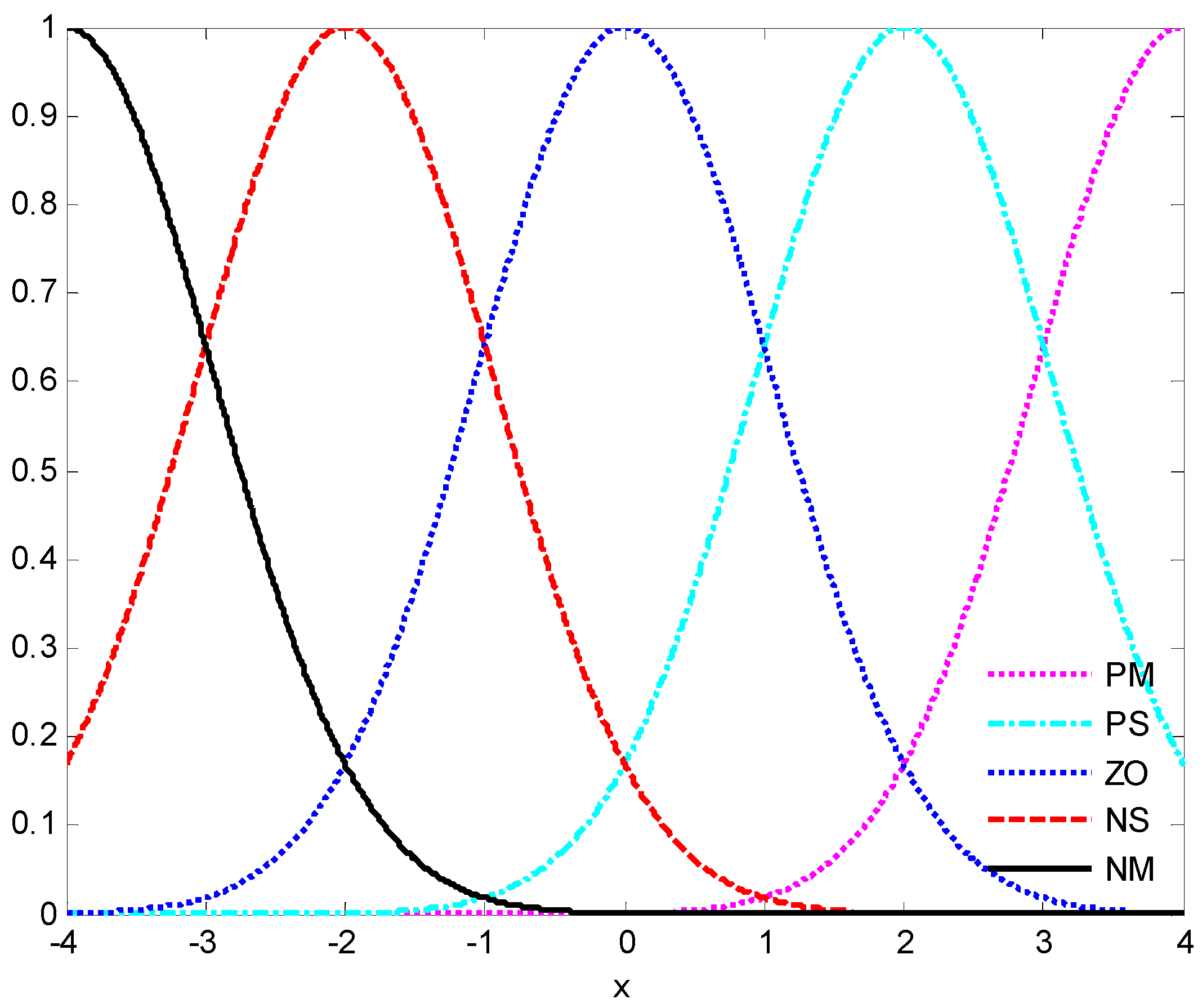In addition, $NM$, $NS$, $ZO$, $PS$, and $PM$ represent negative middle, negative small, zero, positive small, and positive middle with the center points being pointed as −4, −2, 0, 2, and 4, respectively. Accordingly, the fuzzy membership functions are denoted as ${\mu }_{NM}=\exp ({[(x_i-4)/1.5]}^2)$, ${\mu }_{NS}=\exp ({[(x_i-2)/1.5]}^2)$, ${\mu }_{ZO}=\exp ({[(x_i)/1.5]}^2)$, ${\mu }_{PS}=\exp ({[(x_i+2)/1.5]}^2)$ and ${\mu }_{PM}=\exp ({[(x_i+4)/1.5]}^2)$, $i=1,2,3$, respectively. The curves of fuzzy membership functions are shown in Figure 1. Take design parameters and initial conditions as: $\vartheta =0.09$, $c_1=2.7$, $c_2=1.5$, $c_3=1.0$, ${\epsilon }_1^{*}=1.2$, ${\epsilon }_2^{*}=5.5$, ${\mu }_3^{*}=4$, ${\eta }_1={\eta }_2={\eta }_3={10}^{-3}$, ${\mathbf{\Phi }}_1=\mathrm{diag}\{85\}$, ${\mathbf{\Phi }}_2=\mathrm{diag}\{1\}$, ${\mathbf{\Phi }}_3=\mathrm{diag}\{40\}$, ${\tau }_2={\tau }_3=0.02$, ${\pi }_3=5.0$, ${[x_1(0),x_2(0),x_3(0)]}^T={[1.0,0.5,0]}^T$, $y_{2d}(0)=y_{3d}(0)=0$, ${\widehat{\mathit{\theta }}}_1^0(0)={\widehat{\mathit{\theta }}}_2^0(0)={\widehat{\mathit{\theta }}}_3^0(0)=\mathbf{0.0}{\mathbf{2}}_5$, ${\widehat{\delta }}_3^0(0)=0.01$.

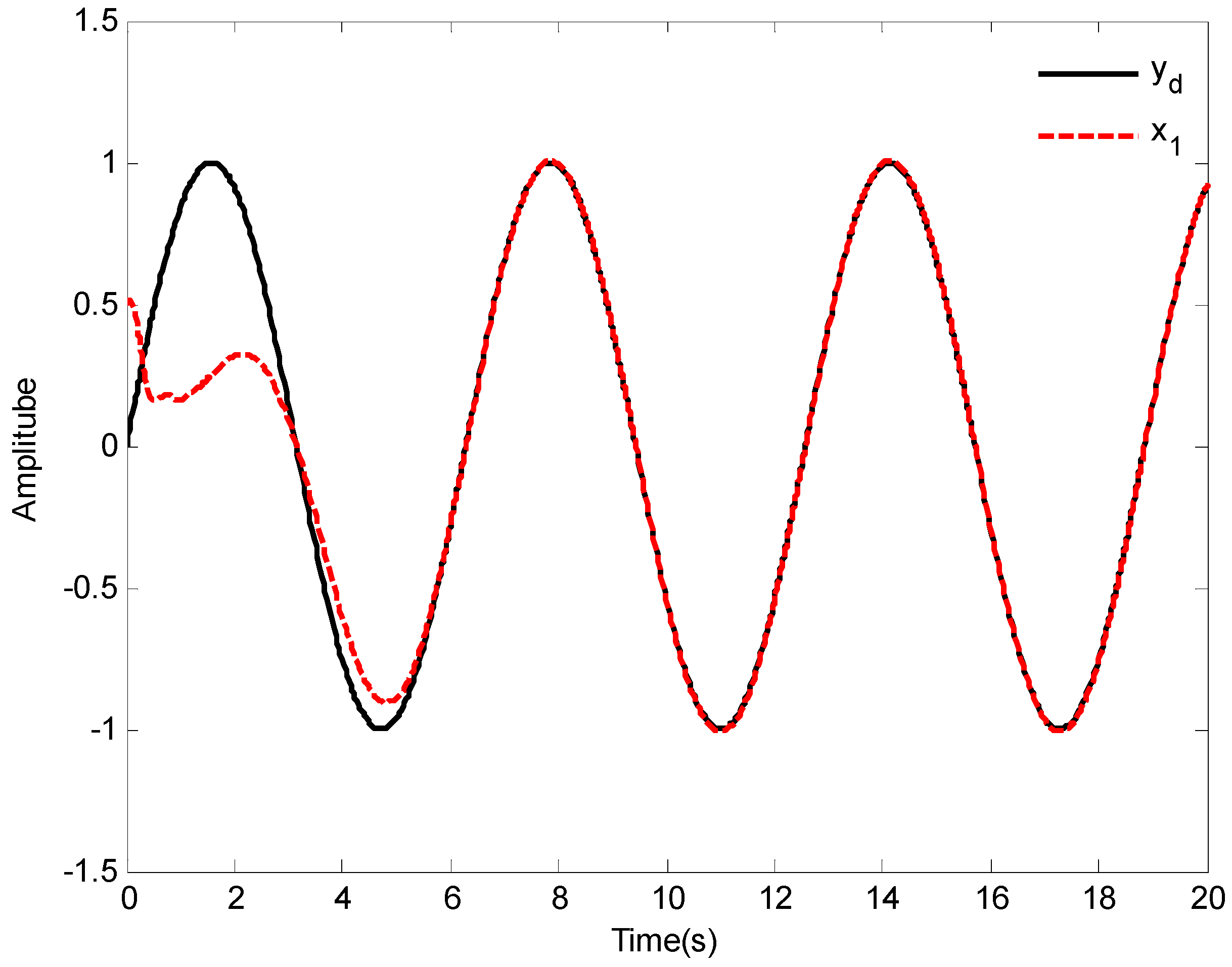
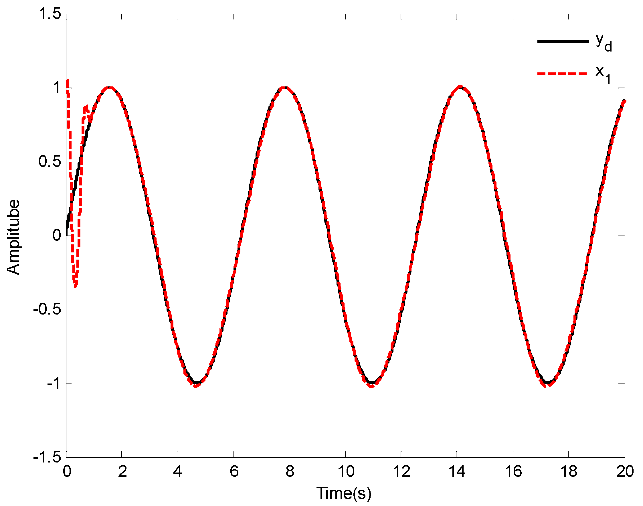
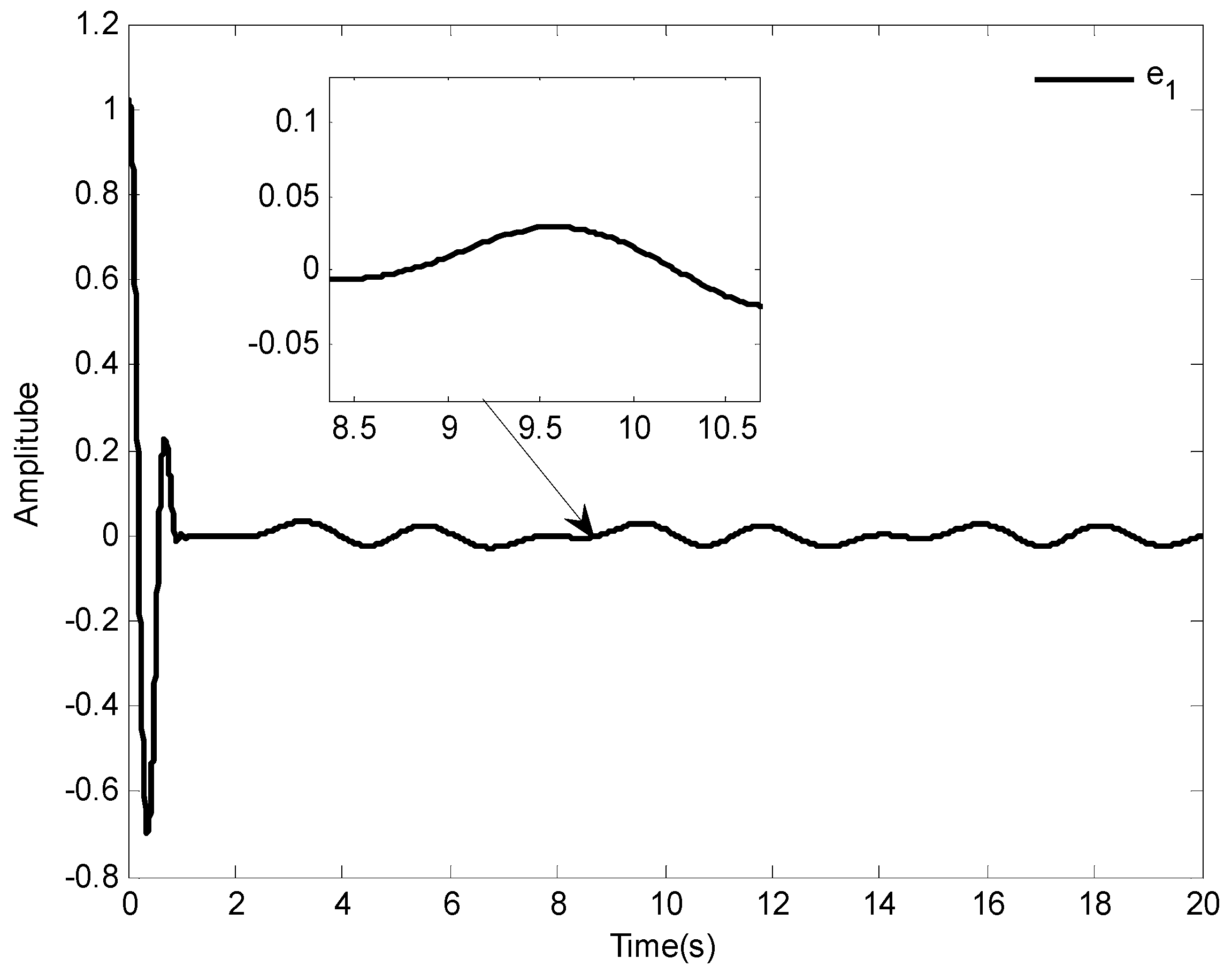
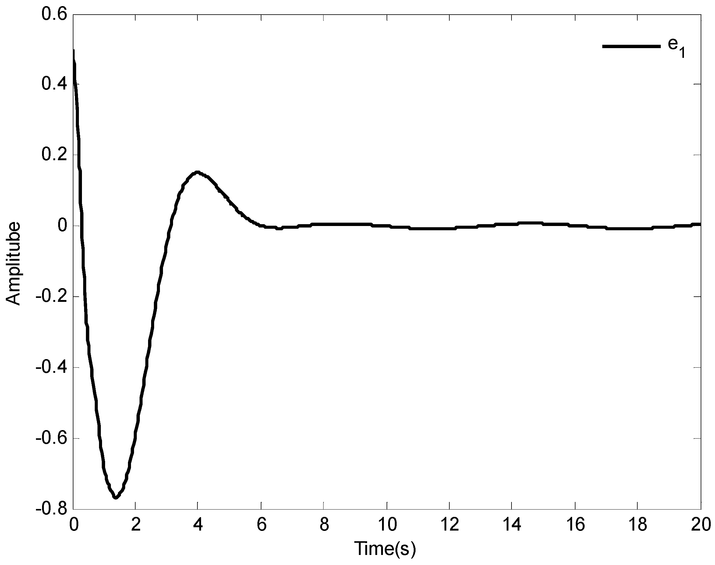
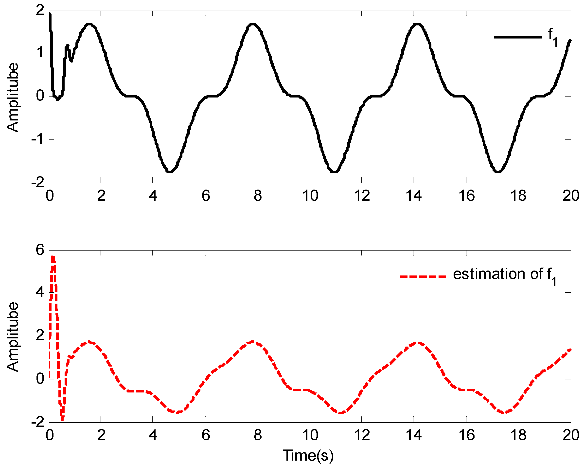
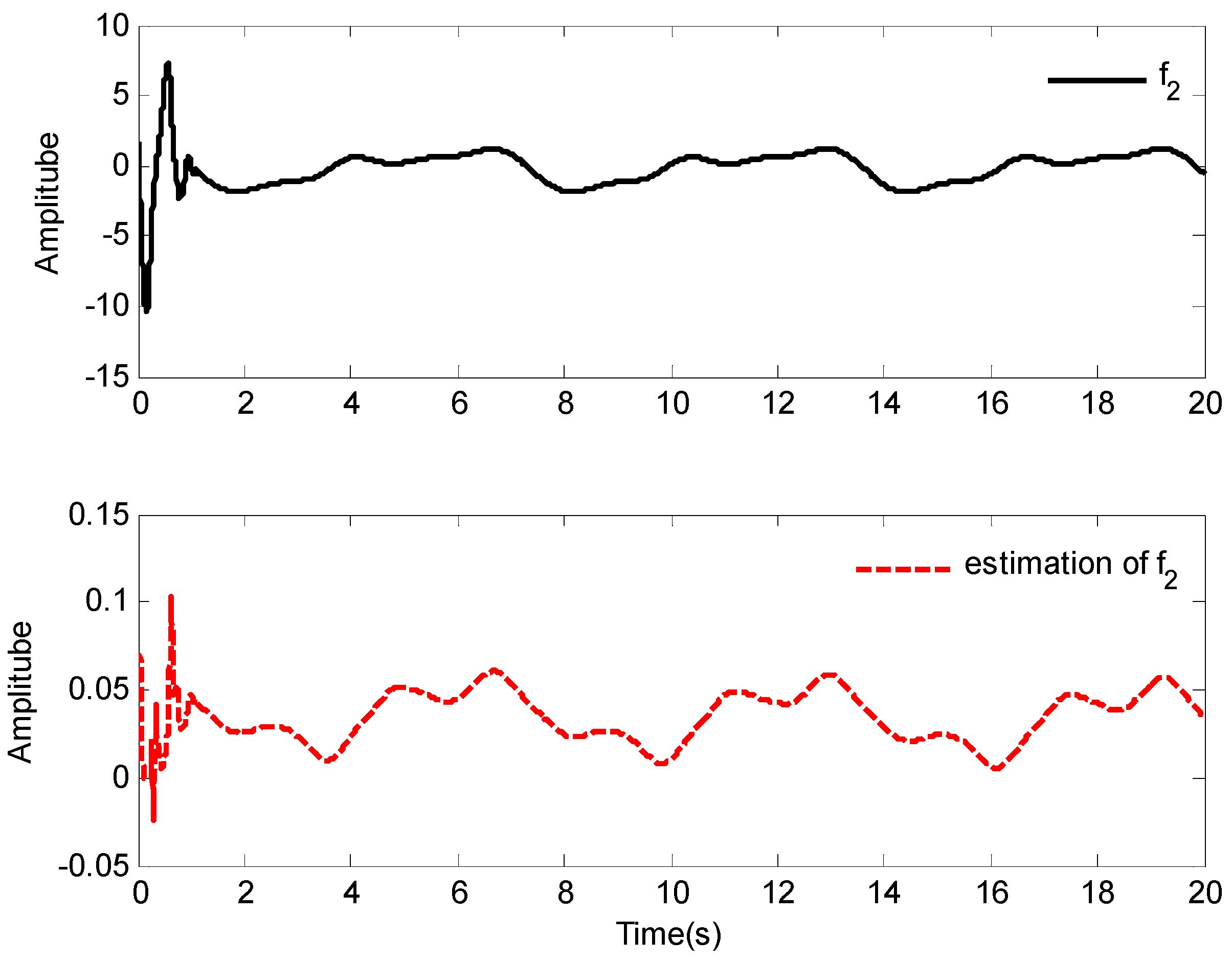
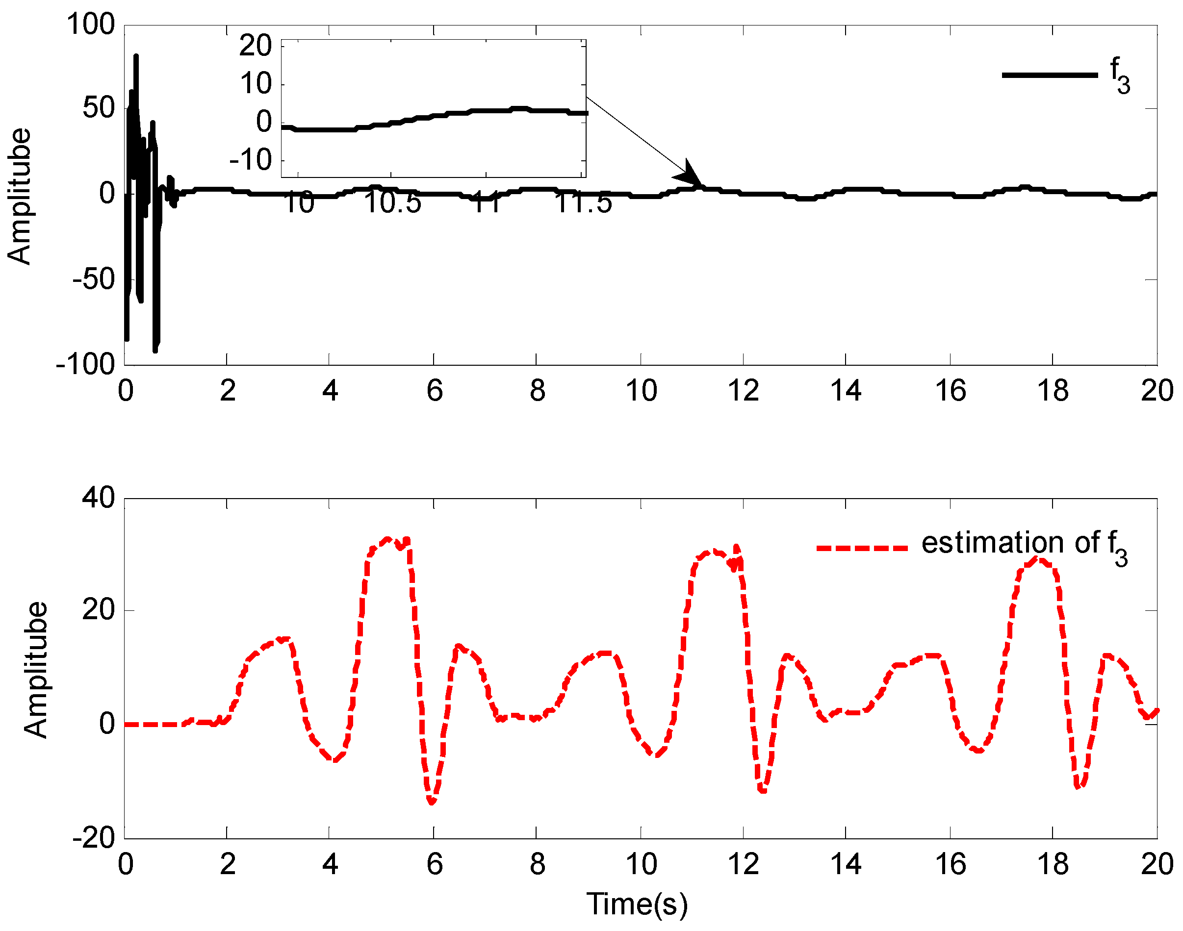
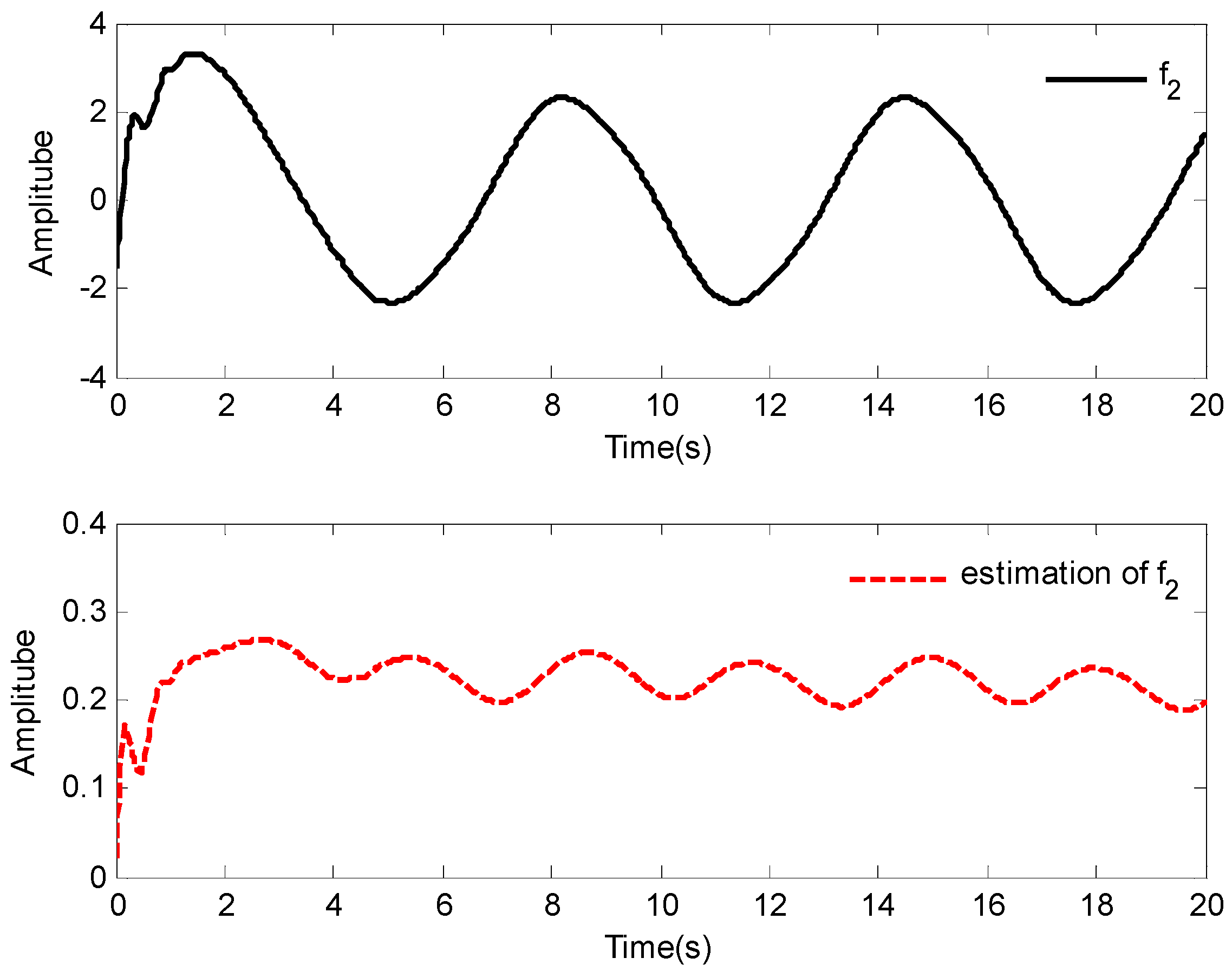
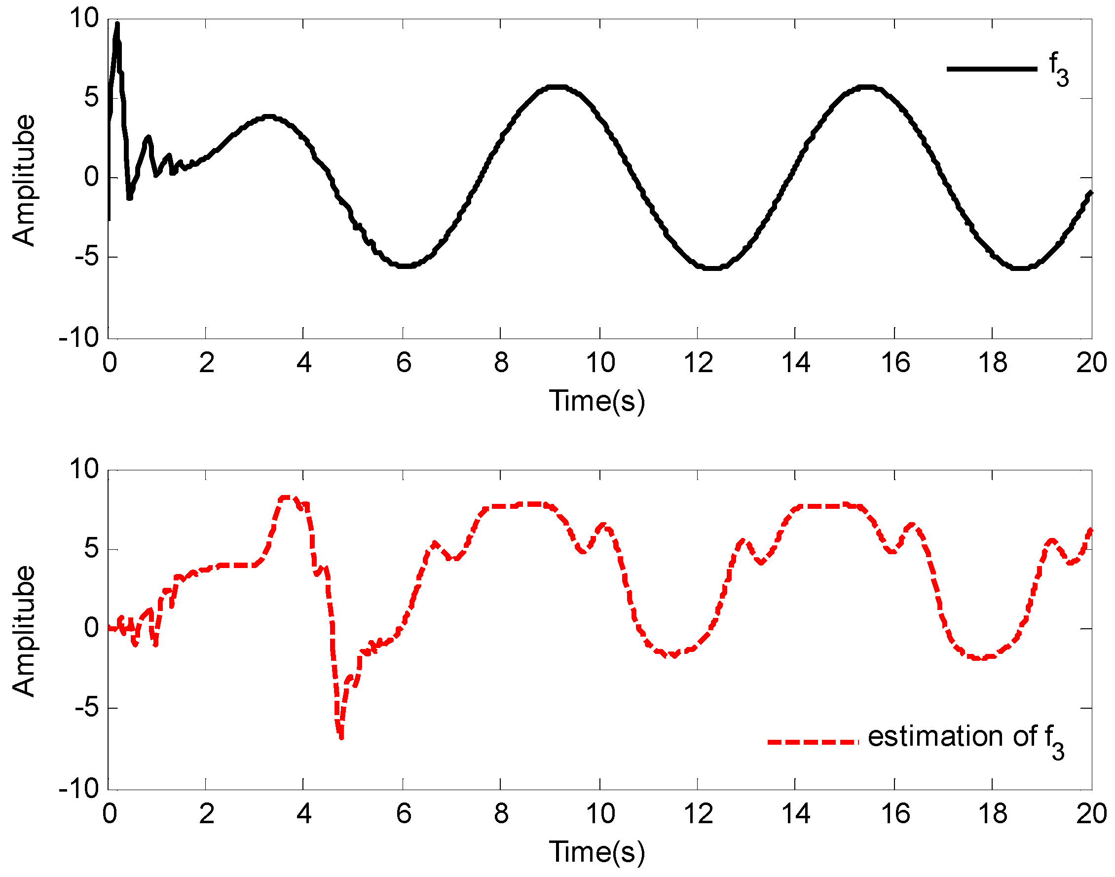
The simulation results of Case 1 are shown in Figure 2, Figure 3, Figure 4, Figure 5, Figure 6, Figure 7, Figure 8 and Figure 9. It is found from Figure 2 and Figure 3 that the excellent tracking performance can be achieved after a short transit process. Furthermore, the curves of nonlinear functions $f_1$, $f_2$, $f_3$ and their estimates ${\widehat{f}}_1$, ${\widehat{f}}_2$, ${\widehat{f}}_3$ are shown in Figure 4, Figure 5 and Figure 6, respectively. 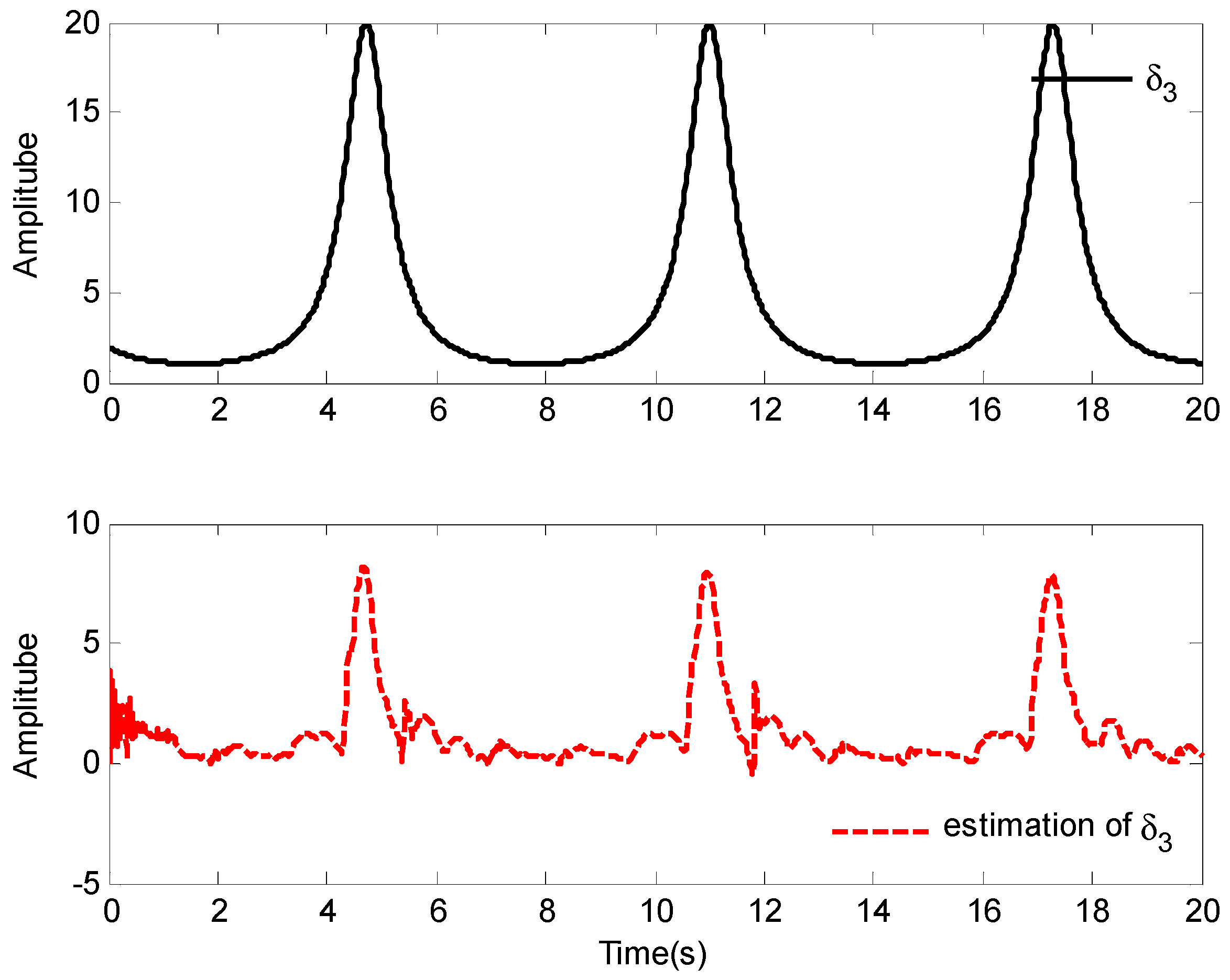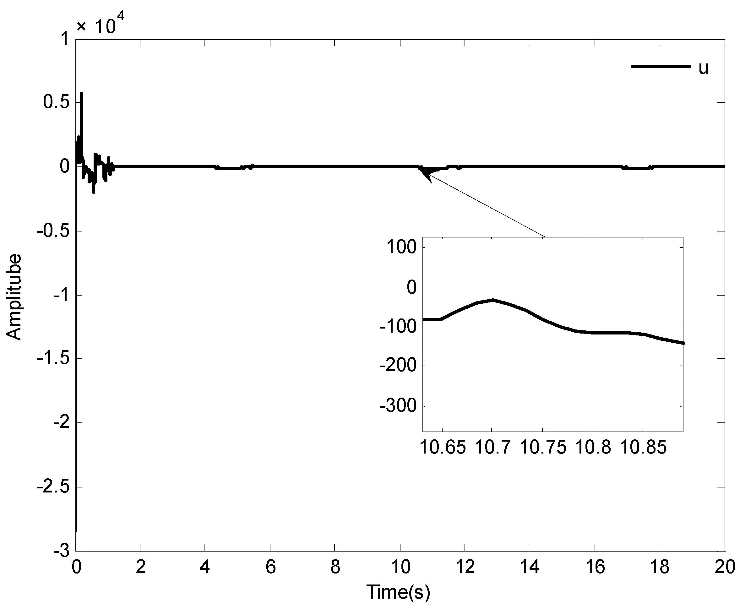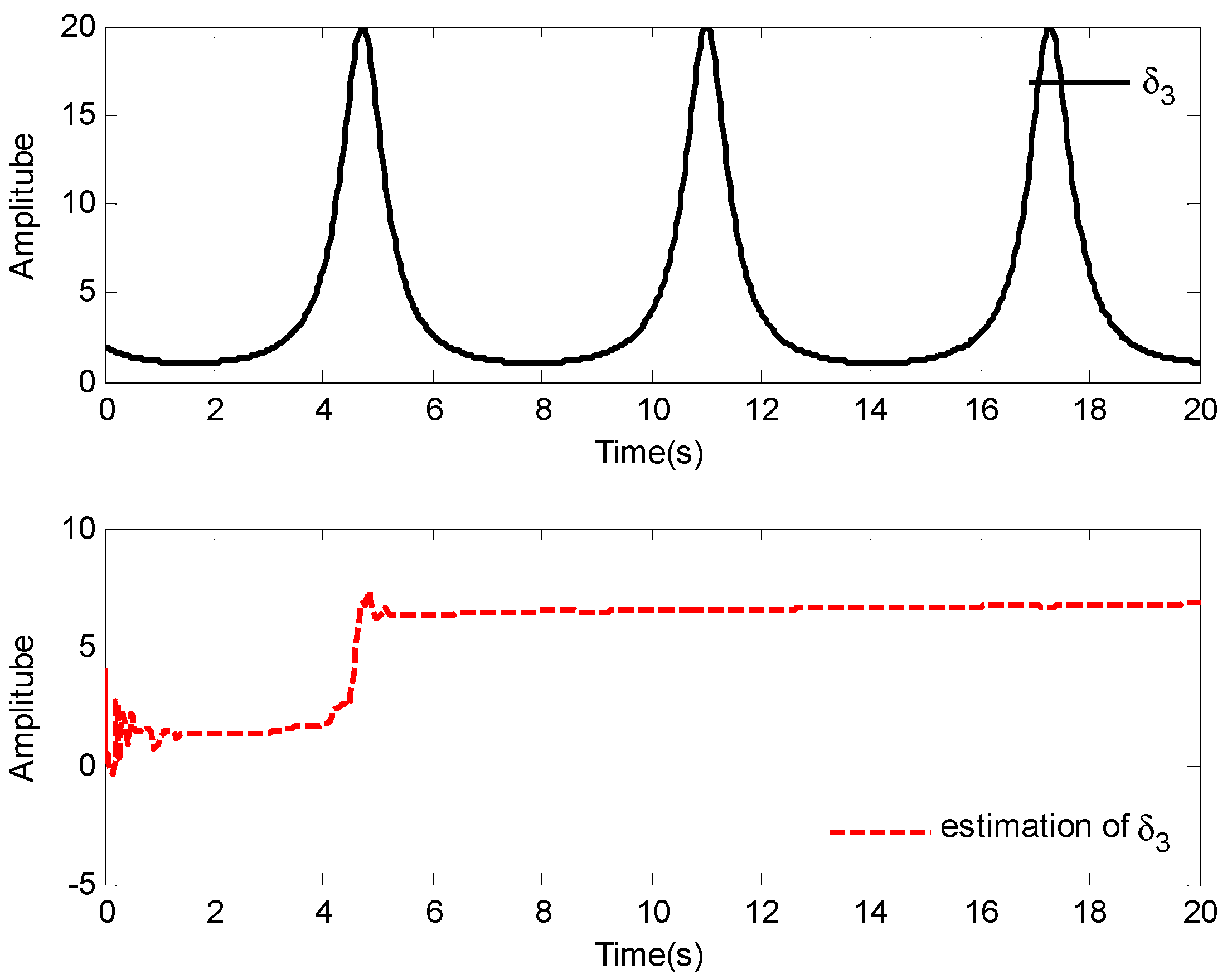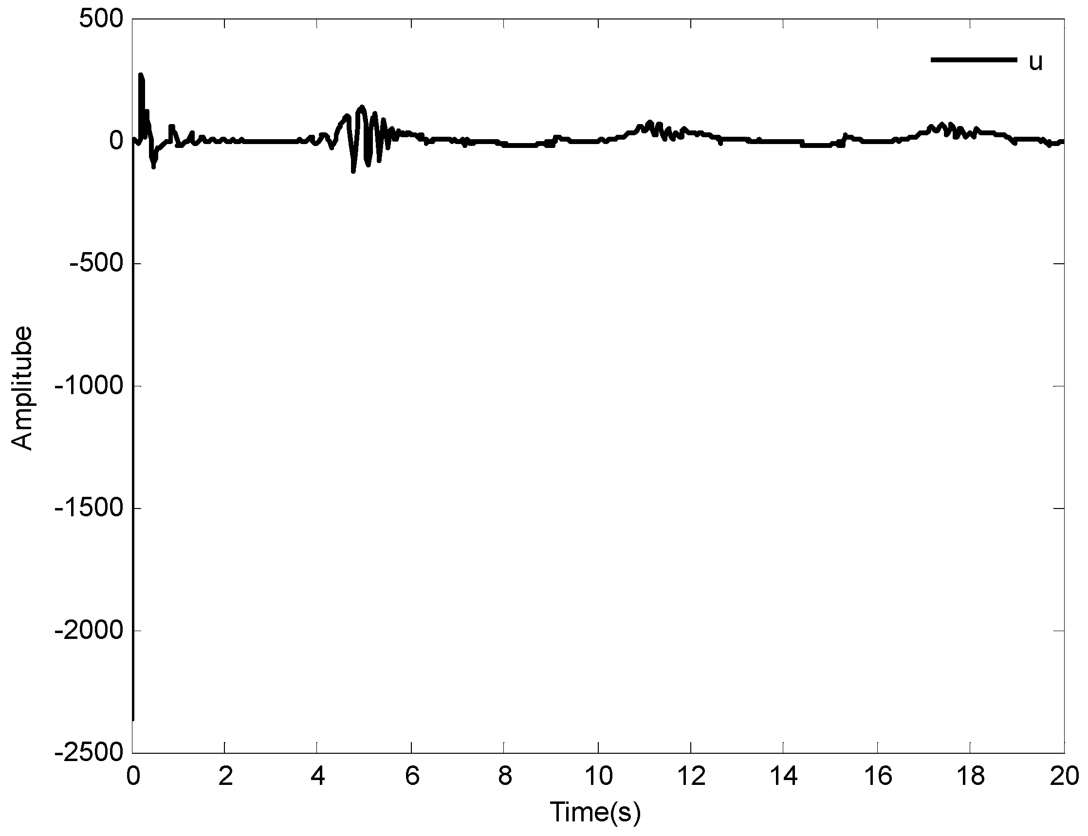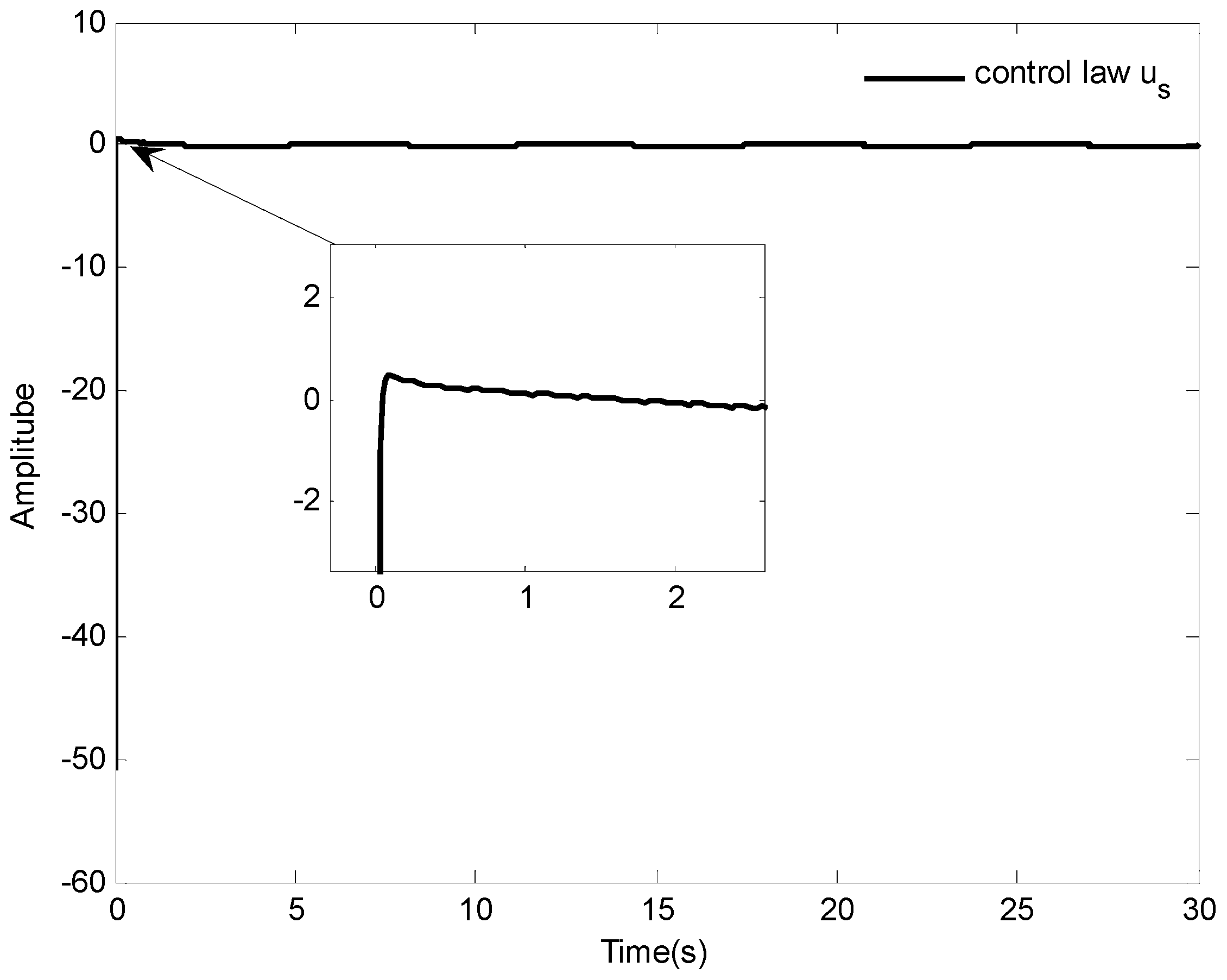Figure 7 gives the curves of ${\delta }_3$ and its estimate ${\widehat{\delta }}_3$, and the control input $u(t)$ is displayed in Figure 8. Because of the initial values are randomly selected, the amplitude of the estimated value of functions $f_2$, $f_3$, and ${\delta }_3$ are greatly reduced compared with the actual value, which also shows that the control laws designed in this paper are effective from another point of view.

Case 2. Consider a one-link manipulator actuated by a brush dc [9], the dynamic of the system is described as:

$$\{\begin{array}{l}C\ddot{p}+A\dot{p}+L\sin (p)=I+d_I\\ Q\dot{I}=-RI-K_m\dot{p}+U\end{array}$$

(63)

where $p$, $\dot{p}$ and $\ddot{p}$ are the link angular position, velocity and acceleration, respectively. $I$ is the motor current, $d_I$ is the stochastic disturbance. $U$ is the input voltage. The parameters of system (62) are given as $C=A=Q=1$, $R=0.5$, $L=2.2$, and $K_m=5$.

Let $x_1=p$, $x_2=\dot{p}$, $x_3=\ddot{p}$ and $\upsilon (t)=U$, so system (63) can be rewritten as follows:

$$\{\begin{array}{l}{\dot{x}}_1=x_2\\ {\dot{x}}_2=x_3-2.2\sin (x_1)-x_2+4\sin (t)\\ {\dot{x}}_3=\upsilon (t)-5x_2-0.5x_3\\ y=x_1\end{array}$$

(64)

Compared with system (1), we have $f_1=0$, $f_2=-2.2\sin (x_1)-x_2+4\sin (t)$, $f_3=-5x_2-0.5x_3$ and ${\Delta }_3\left({\overline{\mathit{x}}}_3(t)\right)=0$. Due to the nonlinear function $f_1=0$, the adaptation law ${\dot{\widehat{\mathit{\theta }}}}_1$ will not appear in the control design. The actuator fault model is considered as (2).

The initial conditions are given as ${[x_1(0),x_2(0),x_3(0)]}^T={[0.5,0.5,0.5]}^T$, the reference signal is given as $y_d=\sin (t)(1-e^{-0.1t^2})$. Some simulation parameters are set as: $\vartheta =0.15$, ${\eta }_2={\eta }_3=0.05$, ${\tau }_2=0.01$, ${\tau }_3=0.15$. Other parameters are the same as in Case 1. The simulation results are depicted in Figure 9, Figure 10, Figure 11, Figure 12, Figure 13 and Figure 14.

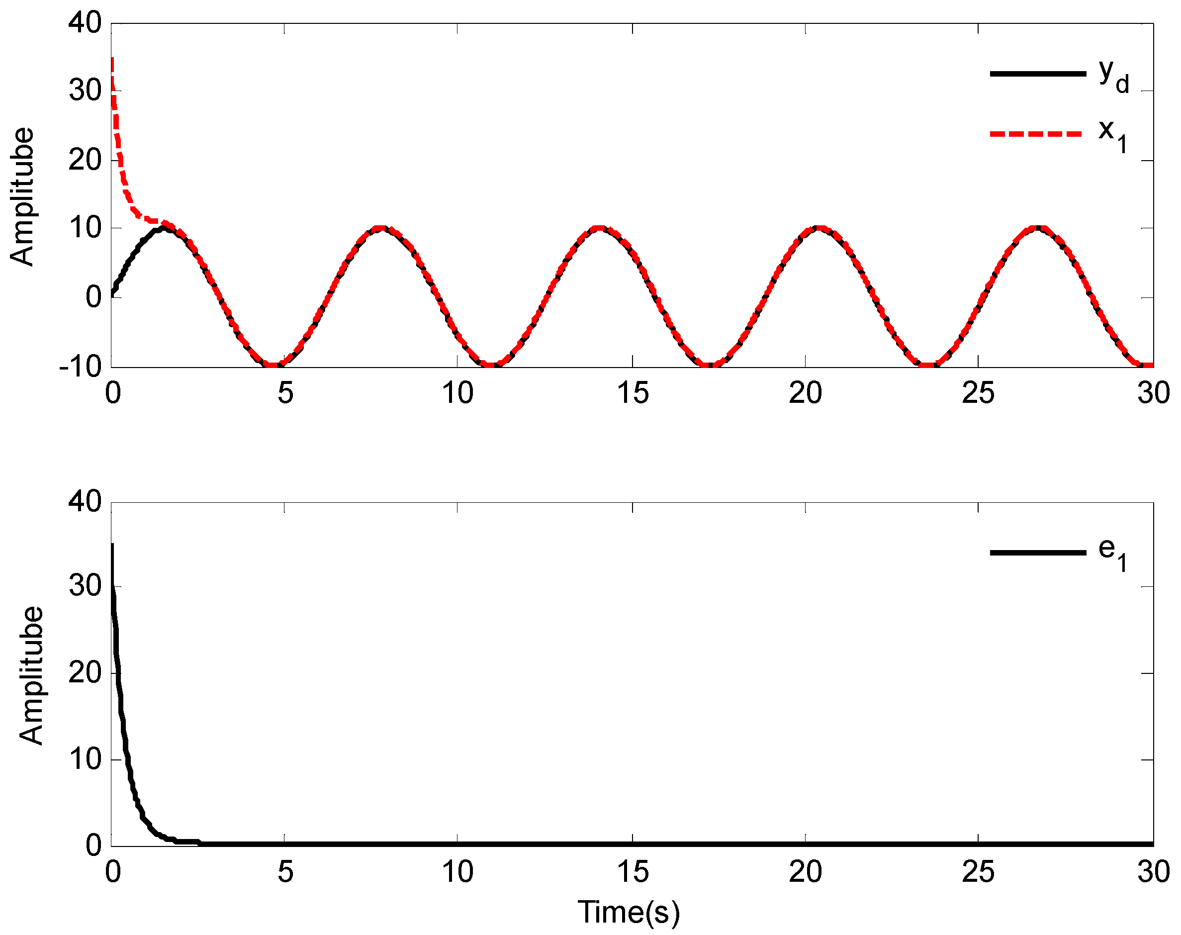
The tracking results and tracking error are shown in Figure 9 and Figure 10, respectively. It is obviously found that the one-link manipulator actuated by a brush dc can obtain good tracking performance based on the application of the adaptive fuzzy dynamic surface control scheme proposed in this paper. Additionally, the nonlinear functions $f_2$, $f_3$ and their estimates ${\widehat{f}}_2$, ${\widehat{f}}_3$ are shown in Figure 11 and Figure 12, respectively, and the curves of ${\delta }_3$ and its estimate ${\widehat{\delta }}_3$ is shown in Figure 13. The control input $u(t)$ is displayed in Figure 14. Similar to Case 1, due to the initial values being randomly selected, it can be found that the amplitude of the estimated value of functions $f_2$, $f_3$, and ${\delta }_3$ are greatly reduced compared with the actual value, which also implies that the control laws designed in this paper are effective from another point of view. Moreover, although the system considered is different, fairly good control performance can still be obtained by using the designed control laws.

Case 3. To further illustrate the effectiveness of the designed control law in practical system application, the system in [44] is considered. According to the description of [44], the model of ship can be rewritten as:

$$\{\begin{array}{l}{\dot{x}}_1=x_2\\ {\dot{x}}_2=K_{ns}{\omega }_n^2{u}_s(t)-2\mathit{\xi }{\omega }_n{x}_2-{\omega }_n^2{x}_1\end{array}$$

(65)

where $x_1=\mathsf{\Psi }(t)$, $x_2=\dot{\mathsf{\Psi }}(t)$, $u_s(t)=o(t)$, $K_{ns}=9.5\times {10}^{-7}$, ${\omega }_n=1.25$ and $\mathit{\xi }=0.8$.

In addition, the initial states of system (64) are given as $x_1(0)=35$ and $x_2(0)=0$, the desired reference signal is given as $y_d=10\sin (t)$, the simulation $t=30\hspace{0.17em}\mathrm{s}$, and the other models are the same as [44]. Based the proposed control law of this paper, the simulation results are shown in Figure 15, Figure 16 and Figure 17.

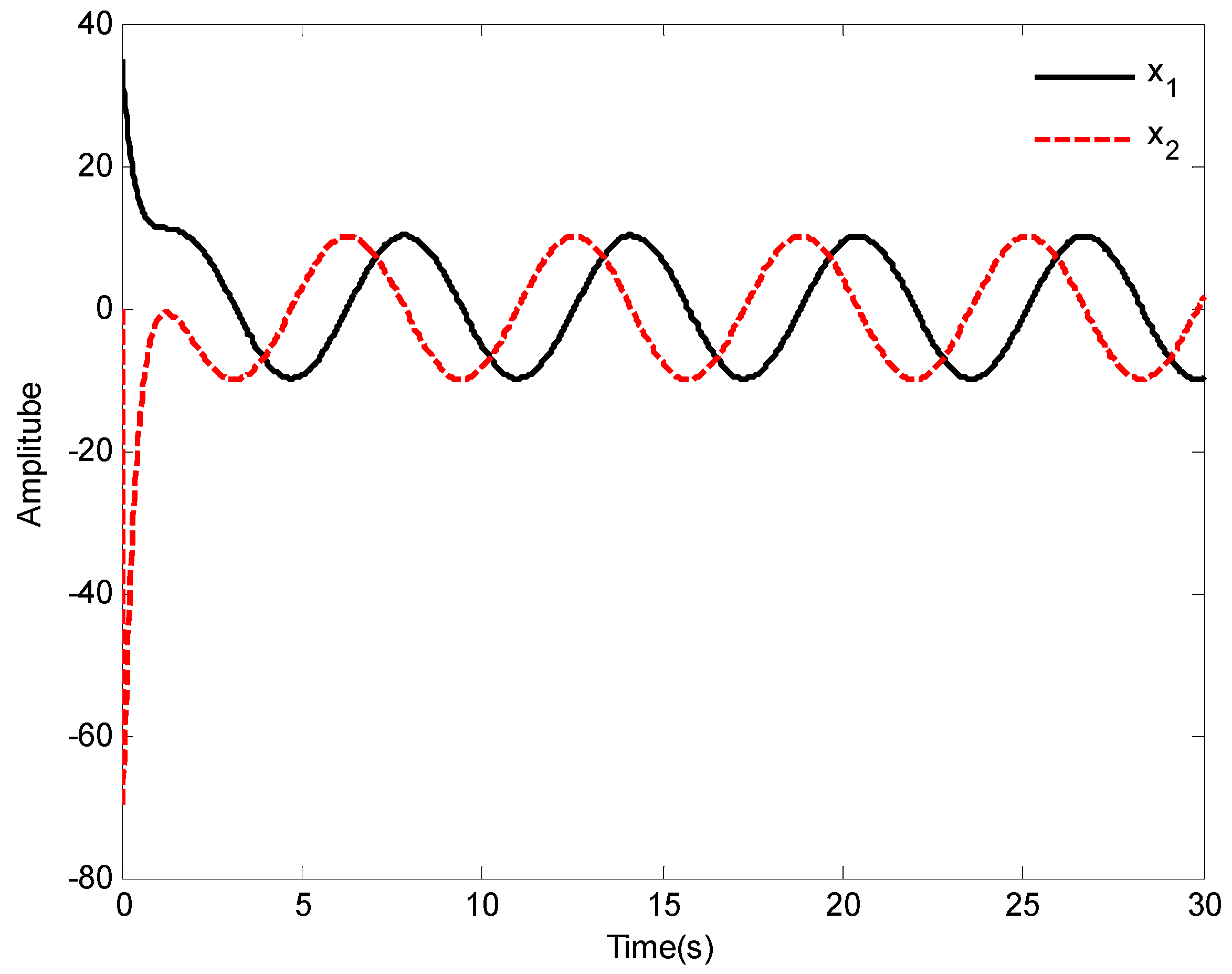
The tracking results and tracking error are displayed in Figure 15. As it is seen in Figure 15, the ship system can obtain good performance under the designed control law, and the tracking error of the system can be very small by selecting appropriate parameters. Moreover, the curves of states and control input are shown in Figure 16 and Figure 17, respectively.

Note 7: Note that the size of the tracking error $e_1$ is affected by the designed parameters $c_i$, ${\eta }_i$, ${\mathbf{\Phi }}_i$, ${\tau }_i$, ${\pi }_n$ and $\vartheta$. Moreover, in the simulation analysis, for other parameters, such as ${\epsilon }_1^{*}$, ${\epsilon }_2^{*}$ and ${\mu }_3^{*}$, are randomly selected, which increases the conservatism of the results to a certain extent. In order to reduce conservatism, we can improve the approximation ability of fuzzy system to nonlinear dynamics by setting the initial value. We can also find the optimal parameters by introducing the optimization method.

6. Conclusions

This paper discusses the tracking control problem of an uncertain nonlinear system with actuator faults by using the adaptive fuzzy control law. The fuzzy logic systems are considered to approximate the uncertain nonlinear functions, and then an adaptive fuzzy dynamic surface control law is proposed. Based on the dynamic surface control technique, the problem of the “explosion of complexity” can be overcome. The simulation results illustrate the effectiveness of the proposed control law. It has been proved that: (a) all of the signals in the closed-loop system are semi-global bounded, (b) the tracking error of the system can converge to a small neighborhood of the origin by adjusting the control law parameters, and (c) fairly good control performance is achieved despite the existence of the actuator fault and uncertain nonlinear dynamics in the system.

The extension of the proposed control law to more complex systems, such as pure-feedback systems and large-scale systems with input delays, is the direction of our future work. In addition, we will also focus on the command filter control method to solve the tracking control problem of system (1) with unknown control directions.

References

1. Zhang, B.Y.; Sun, X.X.; Liu, S.G.; Deng, X.F. Distributed fault tolerant model predictive control for multi-unmanned aerial vehicle system. Asian J. Control 2021. [Google Scholar] [CrossRef]
2. Yoo, S.J.; Park, B.S. Quantized feedback control strategy for tracking performance guarantee of nonholonomic mobile robots with uncertain nonlinear dynamics. Appl. Math. Comput. 2021, 407, 126349. [Google Scholar] [CrossRef]
3. Cheng, X.; Zhang, Y.J.; Liu, H.S.; Wollherr, D.; Buss, M. Adaptive neural backstepping control for flexible-joint robot manipulator with bounded torque inputs. Neurocomputing 2021, 458, 70–86. [Google Scholar] [CrossRef]
4. Chen, Z.Y.; Yang, X.H.; Liu, X.P. RBFNN-based nonsingular fast terminal sliding mode control for robotic manipulators including actuator dynamics. Neurocomputing 2019, 362, 72–82. [Google Scholar] [CrossRef]
5. Zhang, R.D. Improved control for industrial systems over model uncertainty: A receding horizon expanded state space control. IEEE Trans. Syst. Man Cybern. Syst. 2020, 50, 1343–1349. [Google Scholar] [CrossRef]
6. Ji, R.H.; Ma, J.; Li, D.Y.; Ge, S.Z.S. Finite-time adaptive output feedback control for mimo nonlinear systems with actuator faults and saturations. IEEE Trans. Fuzzy Syst. 2021, 29, 2256–2270. [Google Scholar] [CrossRef]
7. Peng, J.Z.; Dubay, R. Adaptive fuzzy backstepping control for a class of uncertain nonlinear strict-feedback systems based on dynamic surface control approach. Expert Syst. Appl. 2019, 120, 239–252. [Google Scholar] [CrossRef]
8. Ling, S.; Wang, H.Q.; Liu, P.X.P. Fixed-time adaptive event-triggered tracking control of uncertain nonlinear systems. Nonlinear Dyn. 2020, 100, 3381–3397. [Google Scholar] [CrossRef]
9. Yang, Z.J.; Zhang, H.G. A fuzzy adaptive tracking control for a class of uncertain strick-feedback nonlinear systems with dead-zone input. Neurocomputing 2018, 272, 130–135. [Google Scholar] [CrossRef]
10. Wu, L.B.; Yang, G.H. Adaptive fuzzy tracking control for a class of uncertain nonaffine nonlinear systems with dead-zone inputs. Fuzzy Sets Syst. 2016, 290, 1–21. [Google Scholar] [CrossRef]
11. Jeong, D.M.; Yoo, S.J. Adaptive event-triggered tracking using nonlinear disturbance observer of arbitrarily switched uncertain nonlinear systems in pure-feedback form. Appl. Math. Comput. 2021, 407, 126335. [Google Scholar] [CrossRef]
12. Lin, W.; Wang, Y.J.; Liu, X.L. Asymptotic stabilization of nonlinear systems with long input delay via memoryless feedback: A linearization method. Automatica 2021, 130, 109731. [Google Scholar] [CrossRef]
13. Wang, F.; Liu, Z.; Zhang, Y.; Chen, C.L.P. Adaptive quantized fuzzy control of stochastic nonlinear systems with actuator dead-zone. Inf. Sci. 2016, 370, 385–401. [Google Scholar] [CrossRef]
14. Zhao, Y.; Liu, Y.F.; Wen, G.H.; Yu, X.H.; Chen, G.R. Distributed average tracking for lipschitz-type of nonlinear dynamical systems. IEEE Trans. Cybern. 2019, 49, 4140–4152. [Google Scholar] [CrossRef] [PubMed] [Green Version]
15. Deng, X.F.; Zhang, C.; Ge, Y. Adaptive neural network dynamic surface control of uncertain strict-feedback nonlinear systems with unknown control direction and unknown actuator fault. J. Frankl. Inst. 2022. [Google Scholar] [CrossRef]
16. Shao, X.F.; Ye, D. Event-based adaptive fuzzy fixed-time control for nonlinear interconnected systems with non-affine nonlinear faults. Fuzzy Sets Syst. 2022, 432, 1–27. [Google Scholar] [CrossRef]
17. Wang, S.X.; Xia, J.W.; Wang, X.L.; Yang, W.J.; Wang, L.Q. Adaptive neural networks control for MIMO nonlinear systems with unmeasured states and unmodeled dynamics. Appl. Math. Comput. 2021, 408, 126369. [Google Scholar] [CrossRef]
18. Li, X.Y.; Wen, C.Y.; Zou, Y. Adaptive backstepping control for fractional-order nonlinear systems with external disturbance and uncertain parameters using smooth control. IEEE Trans. Syst. Man Cybern. Syst. 2021, 51, 7860–7869. [Google Scholar] [CrossRef]
19. Zhao, K.; Song, Y.D.; Chen, C.L.P.; Chen, L. Control of nonlinear systems under dynamic constraints: A unified barrier function-based approach. Automatica 2020, 119, 109102. [Google Scholar] [CrossRef]
20. Meng, F.F.; Zhao, L.; Yu, J.P. Backstepping based adaptive finite-time tracking control of manipulator systems with uncertain parameters and unknown backlash. J. Frankl. Inst. 2020, 357, 11281–11297. [Google Scholar] [CrossRef]
21. Parsa, P.; Akbarzadeh-T, M.R.; Baghbani, F. Command-filtered backstepping robust adaptive emotional control of strict-feedback nonlinear systems with mismatched uncertainties. Inf. Sci. 2021, 579, 434–453. [Google Scholar] [CrossRef]
22. Cui, G.Z.; Yu, J.P.; Wang, Q.G. Finite-time adaptive fuzzy control for mimo nonlinear systems with input saturation via improved command-filtered backstepping. IEEE Trans. Syst. Man Cybern. Syst. 2022, 52, 980–989. [Google Scholar] [CrossRef]
23. Wu, L.B.; Wang, H.; He, X.Q.; Zhang, D.Q. Decentralized adaptive fuzzy tracking control for a class of uncertain large-scale systems with actuator nonlinearities. Appl. Math. Comput. 2018, 332, 390–405. [Google Scholar] [CrossRef]
24. Dastres, H.; Rezaie, B.; Baigzadehnoe, B. Neural-network-based adaptive backstepping control for a class of unknown nonlinear time-delay systems with unknown input saturation. Neurocomputing 2020, 398, 131–152. [Google Scholar] [CrossRef]
25. Liu, H.; Pan, Y.P.; Cao, J.D.; Wang, H.X.; Zhou, Y. Adaptive neural network backstepping control of fractional-order nonlinear systems with actuator faults. IEEE Trans. Neural Netw. Learn. Syst. 2020, 31, 5166–5177. [Google Scholar] [CrossRef]
26. Ma, H.; Liang, H.J.; Zhou, Q.; Ahn, C.K. Adaptive dynamic surface control design for uncertain nonlinear strict-feedback systems with unknown control direction and disturbances. IEEE Trans. Syst. Man Cybern. Syst. 2019, 49, 506–515. [Google Scholar] [CrossRef]
27. Jia, F.J.; Yan, X.; Wang, X.H.; Lu, J.W.; Li, Y.M. Robust adaptive prescribed performance dynamic surface control for uncertain nonlinear pure-feedback systems. J. Frankl. Inst. 2020, 357, 2752–2772. [Google Scholar] [CrossRef]
28. Zhao, K.; Song, Y.D. Removing the feasibility conditions imposed on tracking control designs for state-constrained strict-feedback systems. IEEE Trans. Autom. Control 2019, 64, 1265–1272. [Google Scholar] [CrossRef]
29. Edalati, L.; Sedigh, A.K.; Shooredeli, M.A.; Moarefianpour, A. Adaptive fuzzy dynamic surface control of nonlinear systems with input saturation and time-varying output constraints. Mech. Syst. Signal Processing 2018, 100, 311–329. [Google Scholar] [CrossRef]
30. Rahmani, Z.; Baigzadehnoe, B.; Rezaie, B. Tracking control of a class of nonlinear systems with output delay based on adaptive fuzzy dynamic surface control. Int. J. Syst. Sci. 2020, 51, 1280–1306. [Google Scholar] [CrossRef]
31. Baigzadehnoe, B.; Rahmani, Z.; Khosravi, A.; Rezaie, B. Adaptive decentralized fuzzy output feedback tracking control for a class of nonlinear large-scale systems with input delays. Trans. Inst. Meas. Control 2018, 40, 3534–3548. [Google Scholar] [CrossRef]
32. Baigzadehnoe, B.; Rahmani, Z.; Khosravi, A.; Rezaie, B. Adaptive decentralized fuzzy dynamic surface control scheme for a class of nonlinear large-scale systems with input and interconnection delays. Eur. J. Control 2020, 54, 33–48. [Google Scholar] [CrossRef]
33. Baigzadehnoe, B.; Rahmani, Z.; Khosravi, A.; Rezaie, B. Control of interconnected systems with sensor delay based on decentrialized adaptive neural dynamic surface method. J. Syst. Control Eng. 2021, 235, 751–768. [Google Scholar]
34. Zhou, Z.Y.; Tong, D.B.; Chen, Q.Y.; Zhou, W.N.; Xu, Y.H. Adaptive NN control for nonlinear systems with uncertainty based on dynamic surface control. Neurocomputing 2021, 421, 161–172. [Google Scholar] [CrossRef]
35. Song, S.; Zhang, B.Y.; Song, X.N.; Zhang, Z.Q. Adaptive neuro-fuzzy backstepping dynamic surface control for uncertain fractional-order nonlinear systems. Neurocomputing 2019, 360, 172–184. [Google Scholar] [CrossRef]
36. Shao, X.F.; Ye, D. Fuzzy adaptive event-triggered secure control for stochastic nonlinear high-order mass subject to DoS attacks and actuator faults. IEEE Trans. Fuzzy Syst. 2021, 29, 3812–3821. [Google Scholar] [CrossRef]
37. Lv, M.L.; Yu, W.W.; Baldi, S. The set-invariance paradigm in fuzzy adaptive DSC design of large-scale nonlinear input-constrained systems. IEEE Trans. Syst. Man Cybern. Syst. 2021, 51, 1035–1045. [Google Scholar] [CrossRef]
38. Shojaei, F.; Arefi, M.M.; Khayatian, A.; Karimi, H.R. Observer-based fuzzy adaptive dynamic surface control of uncertain nonstrict feedback systems with unknown control direction and unknown dead-zone. IEEE Trans. Syst. Man Cybern. Syst. 2019, 49, 2340–2351. [Google Scholar] [CrossRef]
39. Wang, H.Q.; Liu, P.X.P.; Zhao, X.D.; Liu, X.P. Adaptive fuzzy finite-time control of nonlinear systems with actuator faults. IEEE Trans. Cybern. 2020, 50, 1786–1797. [Google Scholar] [CrossRef]
40. Zhao, K.J.; Chen, W. Adaptive neural quantized control of MIMO nonlinear systems under actuation faults and time-varying output constraints. IEEE Trans. Neural Netw. Learn. Syst. 2020, 31, 3471–3481. [Google Scholar] [CrossRef]
41. Ma, J.L.; Park, J.H.; Xu, S.Y. Global adaptive control for uncertain nonlinear systems with sensor and actuator faults. IEEE Trans. Syst. Man Cybern. Syst. 2021, 51, 5503–5510. [Google Scholar] [CrossRef]
42. Wang, Z.; Shan, J.J. Fixed-time consensus for uncertain multi-agent systems with actuator faults. J. Frankl. Inst. 2020, 357, 1199–1220. [Google Scholar] [CrossRef]
43. Wang, D.; Huang, J. Neural network-based adaptive dynamic surface control for a class of uncertain nonlinear systems in strict-feedback form. IEEE Trans. Neural Netw. 2005, 16, 195–202. [Google Scholar] [CrossRef]
44. Fortuna, L.; Muscato, G. A roll stabilization system for a monohull ship: Modeling, identification, and adaptive control. IEEE Trans. Control Syst. Technol. 1996, 4, 18–28. [Google Scholar] [CrossRef]
Figure 1. Fuzzy membership functions.
Mathematics 10 01624 g001
Figure 2. The curves of tracking performance.
Mathematics 10 01624 g002
Figure 3. The curve of tracking error.
Mathematics 10 01624 g003
Figure 4. Response of f 1 and f ^ 1 .
Mathematics 10 01624 g004
Figure 5. Response of f 2 and f ^ 2 .
Mathematics 10 01624 g005
Figure 6. Response of f 3 and f ^ 3 .
Mathematics 10 01624 g006
Figure 7. Response of δ 3 and δ ^ 3 .
Mathematics 10 01624 g007
Figure 8. The curve of control input u ( t ) .
Mathematics 10 01624 g008
Figure 9. The curves of tracking performance.
Mathematics 10 01624 g009
Figure 10. The curve of tacking error.
Mathematics 10 01624 g010
Figure 11. Response of f 2 and f ^ 2 .
Mathematics 10 01624 g011
Figure 12. Response of f 3 and f ^ 3 .
Mathematics 10 01624 g012
Figure 13. Response of δ 3 and δ ^ 3 .
Mathematics 10 01624 g013
Figure 14. The curve of control input u ( t ) .
Mathematics 10 01624 g014
Figure 15. The curves of tracking performance and error.
Mathematics 10 01624 g015
Figure 16. The curves of states x 1 and x 2 .
Mathematics 10 01624 g016
Figure 17. The curve of control input u s ( t ) .
Mathematics 10 01624 g017