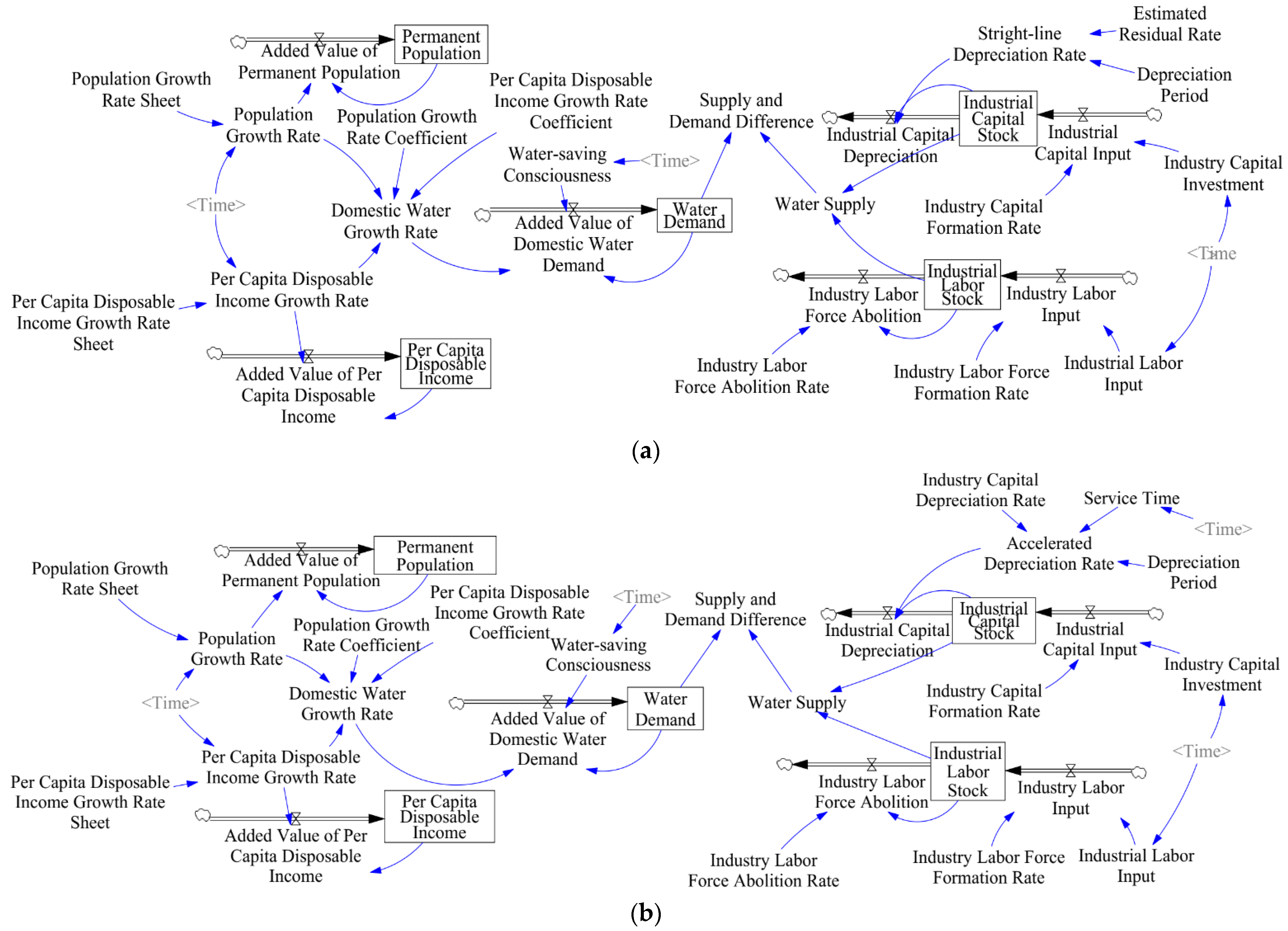
4.3. Simulation
After the model has passed the historical test, it will be further used to predict the supply and demand of domestic water in the next 15 years. Let
and
represent the water supply with the straight-line depreciation method and the sum of years digits method, respectively;
and
represent the investment of the two methods, respectively. The water supply and demand and changes in input factors under the current situation in 2005–2034 are shown in
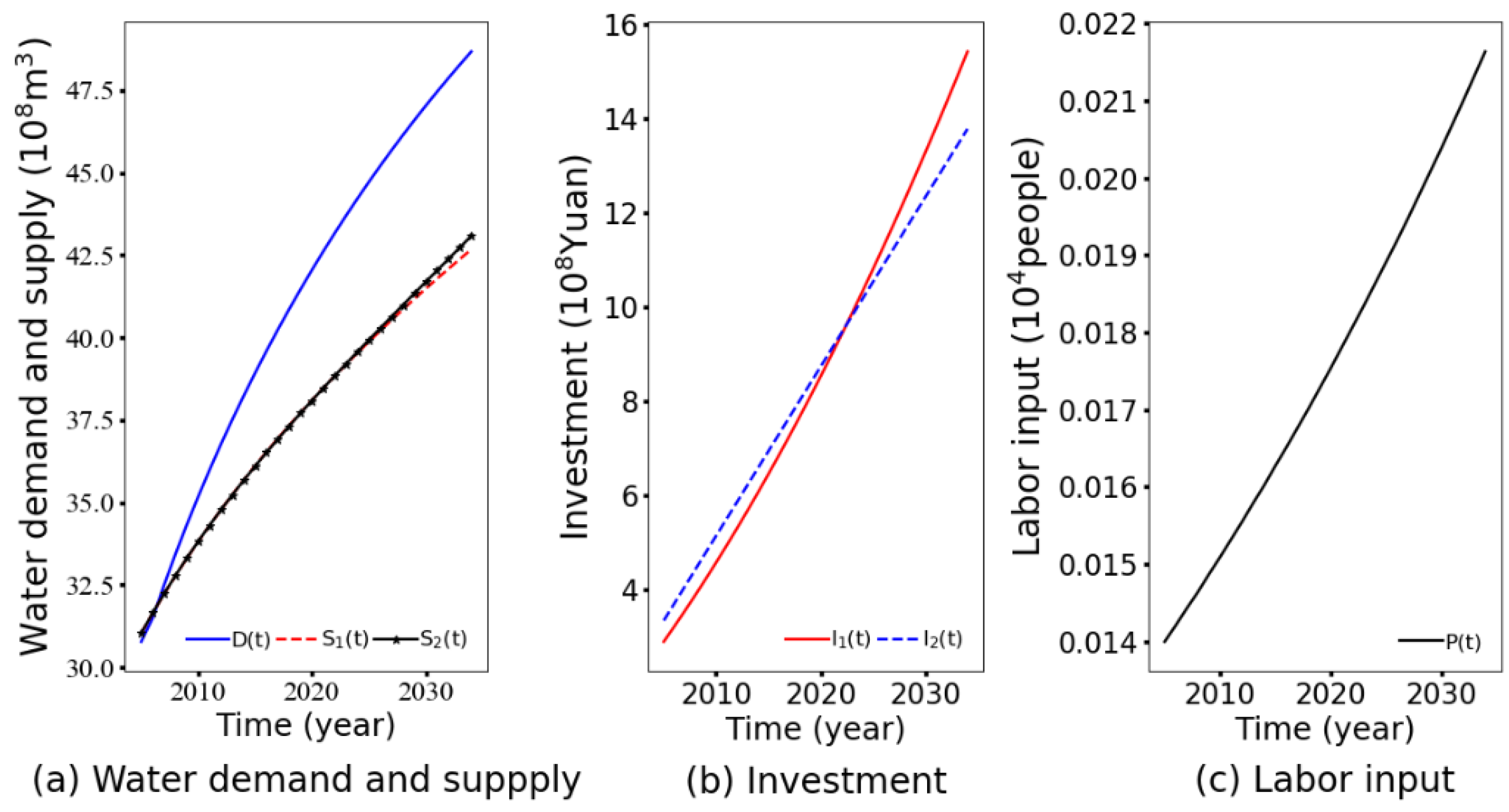
Figure 2.
Figure 2 shows that the growth rates of domestic water supply with the two depreciation methods are less than that of water demand. Supply and demand for both depreciation methods were approximately in balance in 2005–2006, but supply has become increasingly inadequate to meet demand since 2007. By 2034, the water supply with the straight-line method and the sum of years digits method will be
and
less than the water demand, respectively. The investment of the sum of years digits method is more than that of the straight-line depreciation method in 2005–2022, and it is less than straight-line depreciation in 2023–2034. Labor input is increasing in 2005–2034. Regarding the current input level of production factors, increasing investment or labor force is necessary to balance water supply and demand.
Therefore, the investment and the labor input are adjusted as below. The labor input of the straight-line depreciation method is consistent with that of the sum of years digits method.
in 2005 and
in 2006–2034.
Table 5 shows the adjusted investment of the two depreciation methods in 2005–2034.
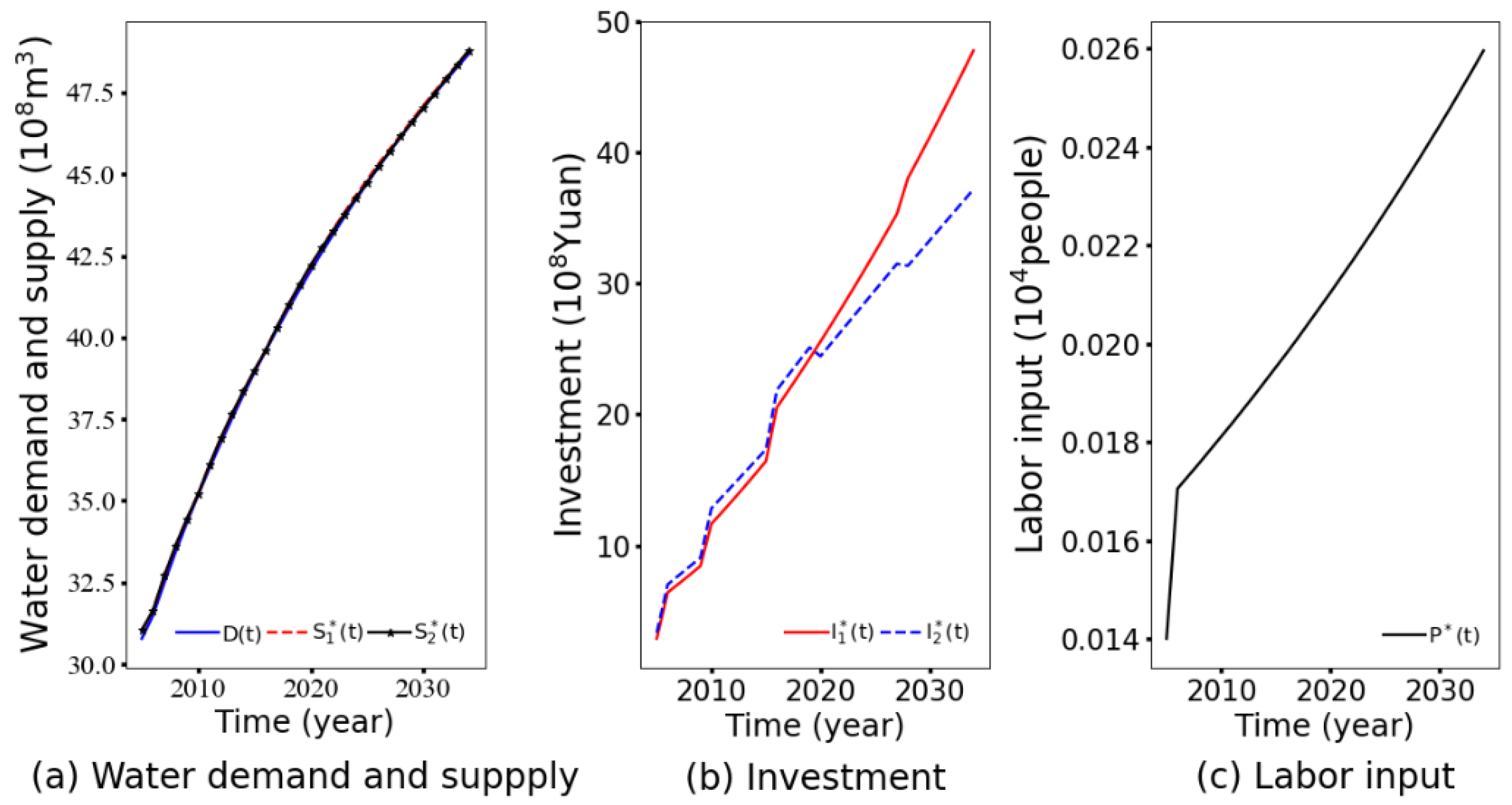
The changes in water supply and improved input factors with the two depreciation methods are shown in
Figure 3.
Figure 3 shows that after the change of input variables, except that the water supply-demand balance with the two methods slightly exceeded
in 2005, the balance in other years was controlled within this value. Moreover, the balance was less than
in 2015–2034. In 2034, the supply is greater than the demand by
with the straight-line depreciation method and
with the sum of years digits method. Compared with the current situation, the improved inputs have dramatically closed the difference between supply and demand. The adjusted investment with the two depreciation methods has increased significantly in the current situation. The investment of the straight-line depreciation method has been shown in a stepwise way. The investment of the sum of years digits method shows a stepwise increase before 2028. Compared with the investment in 2027, it has experienced a certain degree of decline in 2028 and then continues to increase in 2029–2034. The investment of the sum of years digits method is more than that of the straight-line depreciation method from 2005 to 2019, and less than that from 2020 to 2034. The investment difference has increased from 2020 and reaches its maximum in 2034, which is
Yuan. The labor force has also increased significantly compared with the current situation.
4.4. Scenario Simulation
Xu predicted the population change trend of Jiangsu Province after the implementation of the universal two-child policy [
29]. The prediction shows that the population will reach its peak around 2022. The total population will decline year by year from 2023. By 2030, the total population will be roughly equivalent to that when the universal two-child policy was implemented in 2016 [
29]. However, the country introduced the three-child policy in 2021, so the forecast may be affected to some extent.
According to experience, in the year after the birth policy adjustment, the number of births is relatively small and relatively large in the second and third years, then declines in the fourth and fifth years. It is expected that the three-child policy will have a negligible impact on the population change in Jiangsu Province but will not make drastic changes to the long-term trend of population. Therefore, we consider the following scenarios. The total population of Jiangsu Province will decline year by year starting from 2026. It is estimated that the total population in 2034 will be roughly the same as that in 2016, when the universal two-child policy was implemented.
Moreover, we also examine two scenarios of per capita disposable income growth rate after 2020, which are 0.7 times and 1.3 times of the current growth rate, representing low-speed and high-speed income growth, respectively.
Furthermore, two scenarios of the growth rate of water-saving consciousness, , are considered, which are 0.01 and 0.05, representing that the growth rate of water-saving consciousness of residents slowed down and accelerated, respectively. The water demand of residents is positively correlated with the income level. With the increase in income, the sensitivity to water expenditure will generally be reduced, resulting in the rise in water consumption and the weakening of the growth of water-saving consciousness, . However, there may also be another situation. Due to the Chinese Government’s comprehensive promotion of constructing a water-saving society, the residents’ water-saving consciousness grows faster and occurs.
Therefore, four scenarios are obtained by combining the above values of
and
, as shown in
Table 6.
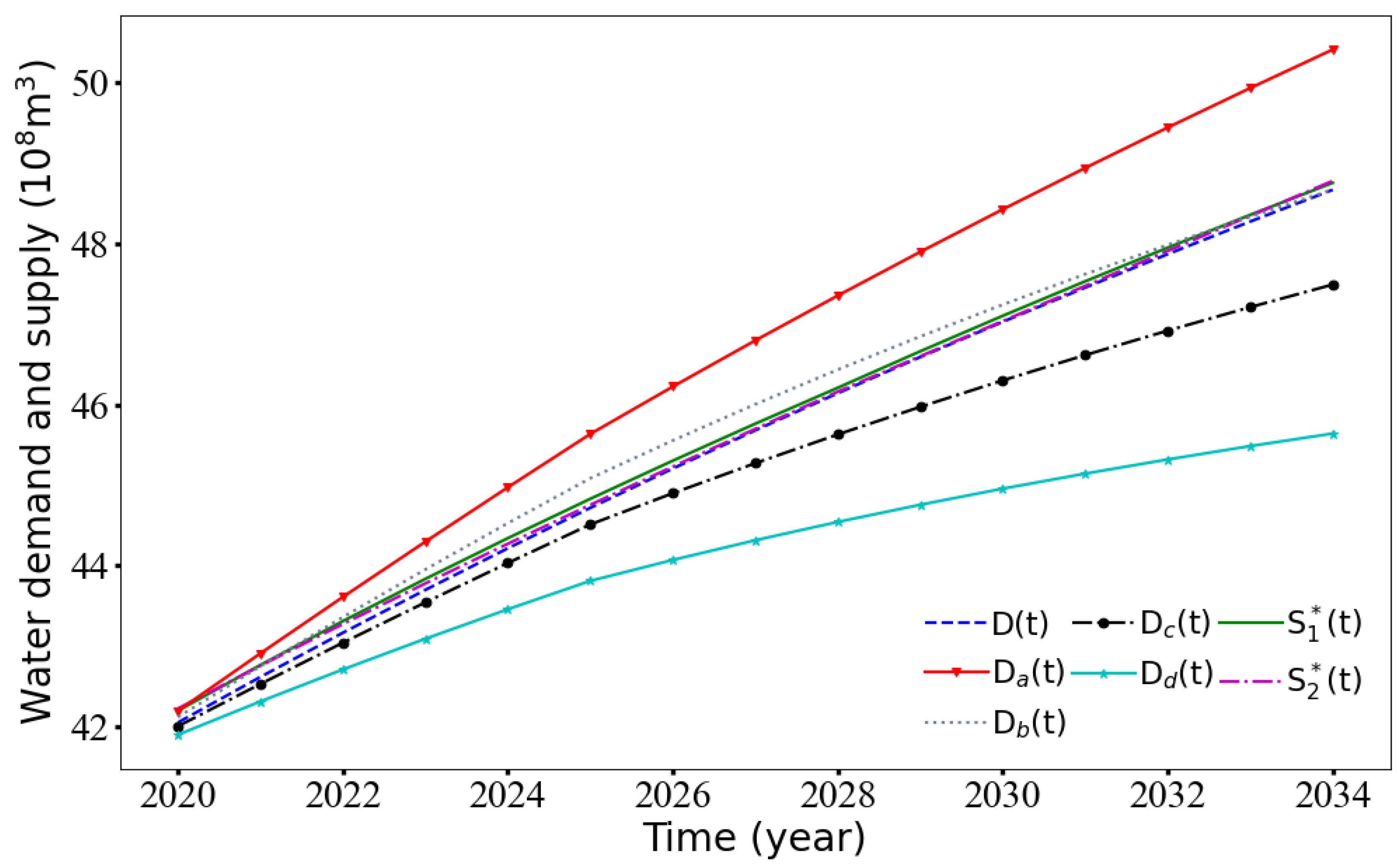
The water demand in Scenario
is represented by
, and the domestic water supply and demand in the four scenarios are shown in
Figure 4.
Figure 4 shows that the water demand under four scenarios and the current water demand are ranked as follows:
. If the production is carried out according to
and
,
and
cannot meet water demand well except that Scenario
is relatively in balance, but there are still some years in short supply. Supply exceeds demand in Scenario
but supply is less than demand in Scenario
and Scenario
. Therefore, it is necessary to adjust investment and labor input further to make the water supply better meet the water demand.
For Scenario , let represent labor input, and represent the investment of the straight-line depreciation method and the sum of years digits method, respectively. Set the value of labor input after debugging as follows. in 2020–2025, in 2026–2034. Since the water consumption population of Jiangsu province is expected to show a negative growth from 2026, it may not be easy to increase labor input, will not be adjusted after 2026, and it is more appropriate to adjust the investment.
The investment is consistent with the current improvement model in 2005–2019, and the adjusted investment in 2020–2034 is set as in
Table 7.
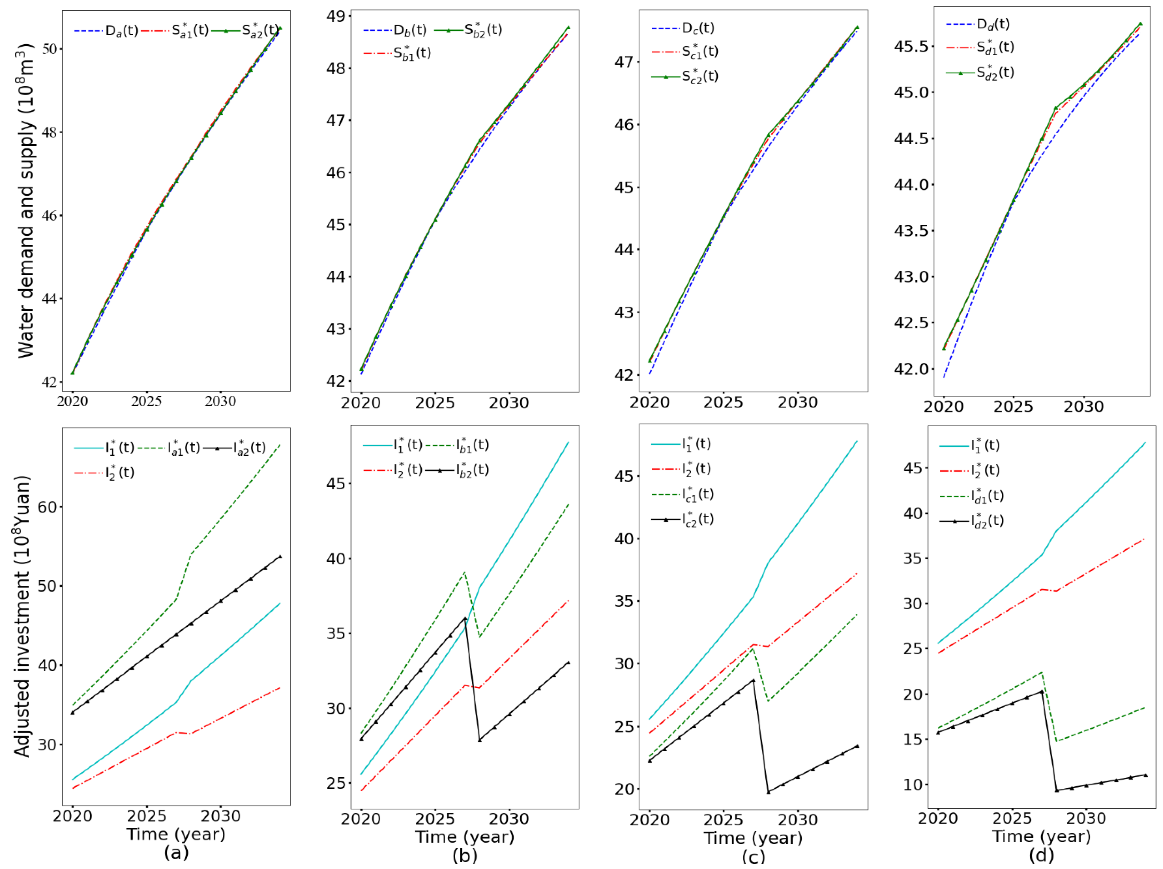
Let
and
represent the water supply of Scenario
with the straight-line depreciation method and the sum of years digits method, respectively. The changes in water demand, supply and adjusted investment under the four scenarios are shown in
Figure 5.
Figure 5a shows that since the water supply is far less than the water demand after 2020 in Scenario
,
and
have increased compared with
and
, respectively, since 2020. Furthermore,
has been greater than
since 2020, and the difference will be
Yuan in 2034. The water supply with the straight-line depreciation method and the sum of years digits method is
and
greater than the water demand, respectively, in 2034.
Figure 5b shows that as the water supply is slightly less than the water demand in 2022–2032 in Scenario
,
and
will be greater than
and
in 2020–2027, but less than
and
in 2028–2034, respectively.
is
Yuan greater than
in 2034. The water supply with the straight-line depreciation method is
greater than the demand in 2034, while the value of the sum of years digits method is
.
Figure 5c shows that since the water supply is greater than the water demand after 2020 in Scenario
,
and
have both experienced a decrease in 2020 and 2028 and then increased. Both
and
are less than the corresponding
and
.
is
Yuan greater than
in 2034. The water supply with the straight-line method and the sum of years digits method is, respectively,
and
greater than the demand in 2034.
Figure 5d shows that as
is less than
in 2020–2034 in Scenario
,
and
have experienced similar but more downward adjustments than
and
in Scenario
in 2020 and 2028, respectively.
is
Yuan greater than
in 2034. The water supply with the straight-line method is
higher than the demand in 2034, and the value of the sum of years digits method is
.
The investment of the two methods has been increasing in a stepwise way in Scenario . With the increase in demand, more investment is needed to make the water supply meet the water demand. However, the investment is not simply increased in Scenarios , and . A timely decision to reduce investment should be made at a time when the accumulation of capital will lead to an oversupply of water by maintaining previous investment levels.
The investment of the sum of years digits method is more than that of the straight-line method in 2005–2019 and less than the latter in 2020–2034 in the four scenarios. The reason is that the depreciation of the sum of years digits method is more than that of the straight-line method in the early period. Therefore, more investment is required to make up for the depreciation than the straight-line method to meet production needs in this period. On the other hand, the depreciation of the sum of years digits method is less than that of the straight-line method in the later period, so the investment is less at this time. The sum of years digits method has the characteristics of larger depreciation in the early period and less depreciation in the later period, which is conducive to timely compensation for the larger loss of fixed assets in the early period.
The differences between the domestic water supply and demand of the two depreciation methods in all the four scenarios have been controlled within . This means that the supply meets the demand fairly well in all the scenarios.
It can provide some references for the regulation of urban domestic water consumption from the model simulation. For example, with the trend of decreasing population, the comparison between Scenario and Scenario shows that the increasing speed of water-saving consciousness can effectively reduce the domestic water demand. By 2034, the gap between supply and demand in Scenario would be less than that in Scenario . Compared with Scenario and Scenario , when the growth rate of water-saving consciousness remains unchanged, the greater the per capita disposable income, the greater the water demand will be. By 2034, is less than . Scenario requires the least water demand in the four scenarios, but this is at the expense of economic development. From the perspective of promoting social development, it is hoped that people’s water-saving consciousness can be strengthened, and meanwhile, the economy can develop rapidly. Therefore, it can be considered that Scenario is the best in the four scenarios. The change trend shows that while ensuring the development of economy, measures such as improving water-saving consciousness can promote the balance of water demand and supply in the long term.


