New Identification Approach and Methods for Plasma Equilibrium Reconstruction in D-Shaped Tokamaks

Abstract

The paper deals with the identification of plasma equilibrium reconstruction in D-shaped tokamaks on the base of plasma external magnetic measurements. The methods of such identification are directed to increase their speed of response when plasma discharges are relatively short, like in the spherical Globus-M2 tokamak (Ioffe Inst., St. Petersburg, Russia). The new approach is first to apply to the plasma discharges data the off-line equilibrium reconstruction algorithm based on the Picard iterations, and obtain the gaps between the plasma boundary and the first wall, and the second is to apply new identification methods to the gap values, producing plasma shape models operating in real time. The inputs for on-line robust identification algorithms are the measurements of magnetic fluxes on magnetic loops, plasma current, and currents in the poloidal field coils measured by the Rogowski loops. The novel on-line high-performance identification algorithms are designed on the base of (i) full-order observer synthesized by linear matrix inequality (LMI) methodology, (ii) static matrix obtained by the least square technique, and (iii) deep neural network. The robust observer is constructed on the base of the LPV plant models which have the novelty that the state vector contains the gaps which are estimated by the observer, using input and output signals. The results of the simulation of the identification systems on the base of experimental data of the Globus-M2 tokamak are presented.

1. Introduction

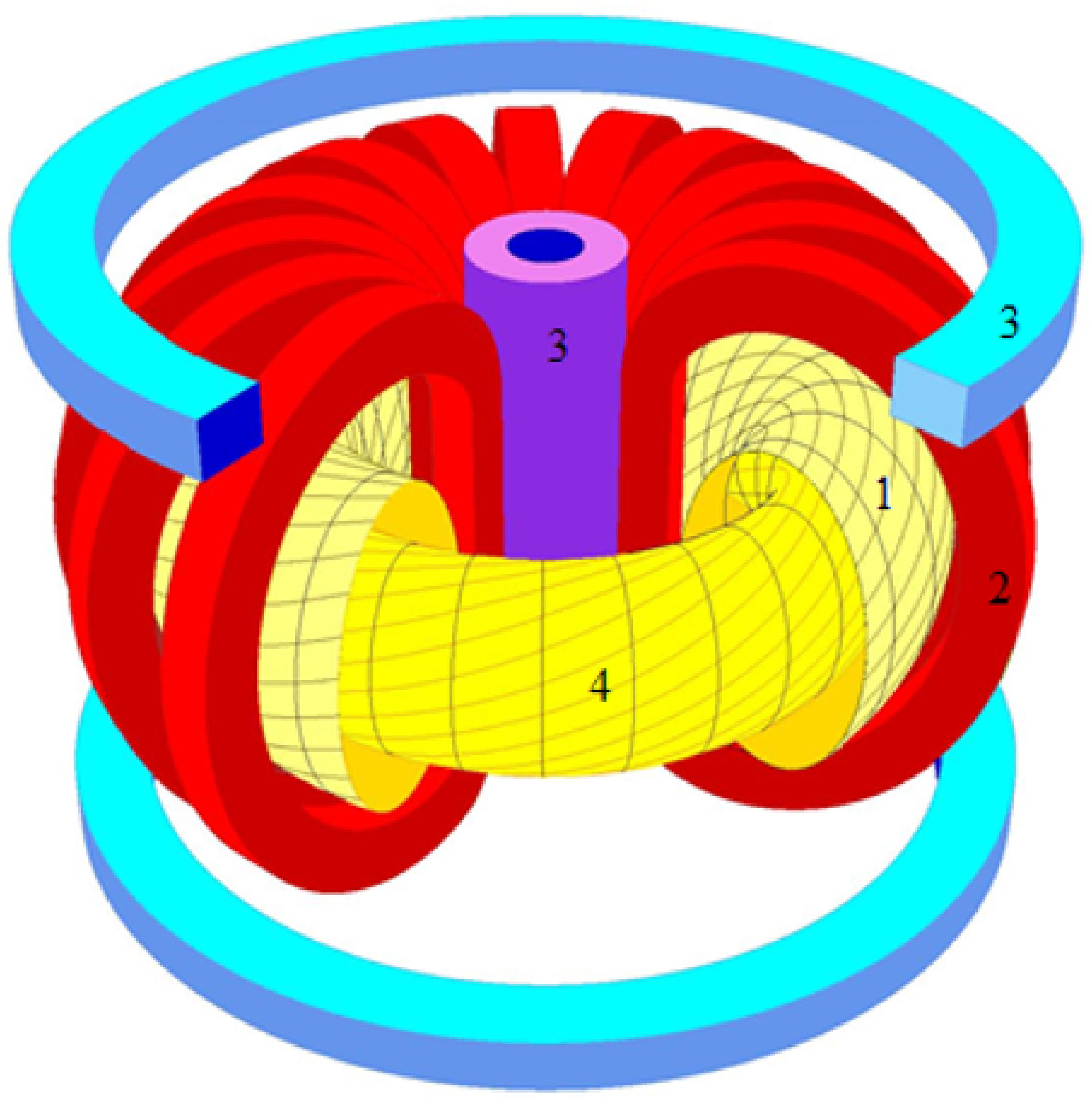
Tokamaks [1], toroidal vessels with magnetic coils (Figure 1), originated at the I.V. Kurchatov Institute of Atomic Energy in the USSR and spread around the world to solve the problem of controlled thermonuclear fusion: obtaining energy from the fusion of the light elements nuclei. The most promising devices for solving this problem are vertically elongated tokamaks with increased gas-kinetic pressure (D-shaped tokamaks) (Figure 1). Plasma (the fourth state of matter) vertically elongated by an external magnetic field is unstable in the vertical direction, and it is necessary to use automatic feedback control systems to keep it near the first tokamak wall.

In our studies, we developed, modeled, and applied control systems of plasma position, current and shape for various tokamaks: ITER (International Thermonuclear Experimental Reactor, Cadarache, France) [2,3], T-15MD (tokamak created at NRC “Kurchatov Institute”, Moscow, Russia, planned to be launched in the near future) [4,5,6], Tuman-3 (toroidal installation with adiabatic compression) [3,4], Globus-M2 (spherical tokamak) [4,7,8] (operating at Ioffe Physics and Technology Institute of RAS, St. Petersburg, Russia), T-11M (operating circular tokamak) [9], and IGNITOR (JSC “SSC RF TRINITI”, Troitsk, Russia) [10].

Since optical reconstruction codes such as OFIT [11] are not available in many tokamaks, the plasma boundary in D-shaped tokamaks usually is not measured directly but rather reconstructed from the external measurements. There are a number of codes which are able to solve that problem, off-line and on-line [12]. The most popular of them are EFIT (equilibrium fitting) [13], which uses the Picard iterations [14] and which is applied on-line on a set of tokamaks, such as DIII-D, NSTX (U.S.), EAST (China), KSTAR (S. Korea) and RTLIUQE [15] used on TCV (Switzerland). These codes were adopted for ITER.

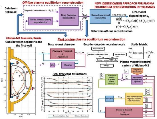
In this work, the new plasma equilibrium reconstruction algorithms are to be inserted into the plasma position, current, and shape feedback control system of the Globus-M2 tokamak. In Figure 2, one can see the digital model of that system [16] where the plasma equilibrium reconstructed algorithm is to be identified by the new methods proposed in the paper.

2. Reconstructing Plasma Equilibria from External Magnetic Measurements

A tokamak is an axially symmetrical device, so the tokamak plasma equilibrium is described in the poloidal plane (r, z), typically in terms of the poloidal magnetic flux distribution $\Psi (r,z)$, which is defined as the flux of the magnetic field vector $\overrightarrow{B}$ through a surface S bounded by the line ($r=const$, $z=const$):

$$\Psi (r,z)=\frac{1}{2\pi }\underset{S}{\int \int }\overrightarrow{B}d\overrightarrow{S}.$$

(1)

The magnetic field lines, along which plasma particles move, lie on the flux surfaces $\Psi (r,z)=const$; therefore, the boundary of the magnetically confined plasma can be found as the largest closed flux surface.

The toroidal current density $J_{\phi }$ in the tokamak is connected with the poloidal flux through the linear second-order partial differential equation [1]:

$$-{\mu }_0^{-1}\left(\frac{\partial }{\partial r}\frac{1}{r}\frac{\partial }{\partial r}+\frac{1}{r}\frac{{\partial }^2}{\partial z^2}\right)\Psi =J_{\phi }.$$

(2)

The boundary conditions for the equation are obtained from the definition and the physical meaning of the poloidal flux:

$${\left.\Psi \right|}_{r=0}=0,{\left.\Psi \right|}_{r=\infty }=0.$$

(3)

When the right-hand side of the Equation (2) is known, it can be solved with the standard numerical methods, for example, using the corresponding Green’s function G [17]:

$$\begin{array}{c}\Psi (r,z)=\int \int J_{\phi }(r^{\prime },z^{\prime })G(r,z,r^{\prime },z^{\prime })d{r}^{\prime }d{z}^{\prime },\\ G(r,z,r^{\prime },z^{\prime })=\frac{{\mu }_0}{\pi }\sqrt{\frac{r{r}^{\prime }}{k^2}}\left(\left(1-\frac{k^2}{2}\right)K\left(k^2\right)-E\left(k^2\right)\right),\end{array}$$

where K and E are the elliptic integrals of the first and the second kind respectively, and

$$k^2=\frac{4r{r}^{\prime }}{{(r+r^{\prime })}^2+{(z-z^{\prime })}^2}.$$

In practice, the plasma current distribution and the induced currents in the conductive Vacuum Vessel (VV) of the tokamak are often not available for real-time reconstruction and must be identified together with the poloidal flux distribution from the external magnetic measurements, which include coil currents $I_1,\dots ,I_{N_c}$, total plasma current $I_p$ measured by Rogowski coils and poloidal flux values $\Psi$ at finite number of points $\left\{(r_1,z_1),\dots ,(r_{N_l},z_{N_l})\right\}$ by magnetic loops outside the plasma.

Hence, the plasma equilibrium reconstruction problem is to find plasma area $S_p$, plasma current distribution $J_p$ and induced current density $J_v$ such that:

$${\chi }^2={\left(I_p-\int J_{p}dS\right)}^2/{\sigma }_p^2+\sum _{j=1}^{N_l}{\left({\Psi }_j-\Psi (r_j,z_j)\right)}^2/{\sigma }_j^2\underset{J_p,J_v}{\to }min,$$

(4)

where ${\sigma }_p$ and ${\sigma }_j$ are uncertainties of the plasma current and poloidal flux at $j\mathrm{th}$ magnetic loop, $\Psi (r,z)$ is the solution of the Equation (2) with boundary conditions (3) and the right-hand side:

$$J_{\phi }(r,z)=\left\{\begin{array}{c}{J}_p,(r,z)\in S_p,\hfill \\ I_k{N}_k/S_k,(r,z)\in S_k,k=1,\dots ,N_c,\hfill \\ J_v(r,z)\in S_v,\hfill \end{array}\right.$$

$S_k$ and $S_v$ are the area occupied by the $k\mathrm{th}$ coil and the VV, respectively, $N_k$ is the number of turns of the $k\mathrm{th}$ coil.

Optionally, coil current measurements may also be considered uncertain and accounted in the functional (4) by terms ${\left(I_k-I_k^{measured}\right)}^2/{\sigma }_{I_k}^2$, $k=1,\dots ,N_c$. The functional may also include other measurements that can be expressed in terms of the currents and the magnetic flux. Finally, as the plasma equilibrium reconstruction problem is ill-posed in the sense of Hadamard, the functional may include a regularization term.

To find the plasma shape in the Globus-M2 tokamak (Figure 3), the flux-current distribution identification (FCDI) code was used [14]. The FCDI code applies the following expression for the plasma toroidal current density, obtained from the plasma force balance equations [1,14]:

$$J_p=r{p}^{\prime }\left(\Psi \right)+\frac{1}{{\mu }_{0}r}F\left(\Psi \right)F^{\prime }\left(\Psi \right).$$

where p is plasma pressure and F is poloidal current defined analogous to poloidal flux (1):

$$F=\frac{{\mu }_0}{2\pi }\underset{S}{\int \int }\overrightarrow{J}d\overrightarrow{S}.$$

The Picard iteration method is used to find the poloidal flux distribution. Since F and p depend only on poloidal flux, on each iteration, the FCDI code approximates the plasma current density by polynomials of the poloidal flux from the previous iteration:

$$\begin{array}{c}{p}^{\prime }\left(\Psi \right)=\sum _{k=0}^{N_p}{c}_k^{\left(p\right)}{\Psi }^k,\\ F\left(\Psi \right)F^{\prime }\left(\Psi \right)=\sum _{k=0}^{N_F}{c}_k^{\left(F\right)}{\Psi }^k.\end{array}$$

Similarly, the VV currents are approximated as a linear combination of some basis functions, for example, orthogonal VV current modes [18]:

$$J_v=\sum _{k=0}^{N_v}{c}_k^{\left(v\right)}{J}_k.$$

The coefficients of the $J_p$ polynomials and the $J_v$ basis function regression are found then by minimizing the error functional (4) which can be written in the matrix form:

$${\chi }^2={\parallel Ac-b\parallel }^2.$$

Here, c is the $N\times 1$ column-vector of the coefficients $c^{\left(p\right)},c^{\left(F\right)},c^{\left(v\right)}$, $N=N_p+N_F+N_v$, A is the $M\times N$ matrix, where M is the number of magnetic measurements used, and b is the $N\times 1$ column-vector. To regularize the problem, the SVD truncation method is used to minimize the quadratic functional [19]. After the coefficients are determined, the corresponding poloidal flux distribution is calculated, which is used for the polynomials construction on the next iteration. The iterations are continued until the error ${\chi }^2$ is sufficiently small or the maximal number of iterations is reached.

3. Experimental Data

The FCDI code was applied to 50 discharges of the Globus-M2 tokamak. For each discharge, there are magnetic measurements available $y^{\left(1\right)},y^{\left(2\right)},\dots ,y^{\left(50\right)}$, which include currents in the 8 control coils (Horizontal Field Coil, Vertical Field Coil, Central Solenoid, Poloidal Field Coil 1, upper and lower sections of the Poloidal Field Coil 2, Poloidal Field Coil 3 and Correcting Coil) (Figure 4), poloidal magnetic flux from 21 loops, vertical dipole magnetic flux (difference between magnetic flux above and below plasma), horizontal dipole magnetic flux (difference between magnetic flux on the left and on the right of the plasma), and quadrupole magnetic flux (expressed as $\psi \left(L_1\right)-\psi \left(L_2\right)+\psi \left(L_3\right)-\psi \left(L_4\right)$, with location of loops $L_1$–$L_4$ shown in Figure 4) so that $y^{\left(i\right)}\in {\mathbb{R}}^{33\times s_i}$, $i\in [1;50]$, where each $s_i=T_i/\tau$, $T_i$ is the duration of the discharge, $\tau$ is the discretization step. Here, the discretization step is the time step between the reconstructed off-line equilibria. It is constrained only by the discretization time of the experimental measurements.

From these data, the FCDI code obtains plasma current distribution and plasma boundary coordinates for the divertor phases of the discharges. The calculated plasma shapes are represented by the positions of 2 strike points ($g_1$, $g_2$) on the VV and values of 4 gaps ($g_3$–$g_6$) between plasma and VV (Figure 4) $g^{\left(1\right)},g^{\left(2\right)},\dots ,g^{\left(50\right)};g^{\left(i\right)}\in {\mathbb{R}}^{6\times s_i}$. The strike points are points of intersection of the poloidal flux isoline, which bounds the plasma and the VV. Their coordinates $g_1$ and $g_2$ are calculated as the distance from point $P_6$ in Figure 4 along the VV. The gap $g_3$ is calculated as the distance between point $P_3$ on the VV outer wall and the plasma boundary on the horizontal line, $g_4$ is the distance between $P_4$ and the plasma boundary on the ${45}^{\circ }$ line, $g_5$ is the distance between $P_5$ and the plasma boundary along the vertical line, and $g_6$ is the distance between point $P_6$ on the VV inner wall and the plasma along the horizontal line. The $g_1$–$g_6$ values describe plasma shape in the LSND (lower single null divertor) configuration, typical for the Globus-M2 tokamak. Other configurations may require different sets of descriptors, but the identification methods described below are applicable all the same.

4. Plasma Model

The plasma dynamics is described by Faraday’s law equations:

$$\frac{d}{dt}\Phi (J_p,I)+RI=U,$$

(5)

and force balance equation

$$\overrightarrow{F}(J_p,I)=0.$$

(6)

The measured fluxes and the plasma shape are determined by currents in the tokamak:

$$\begin{array}{c}\hfill \Psi =\Psi (J_p,I),\\ \hfill g=g(J_p,I).\end{array}$$

(7)

Here, $I={[I_c^{\mathrm{T}},I_v^{\mathrm{T}},I_p]}^{\mathrm{T}}$, $\Phi$, R, and U are respectively the column-vector of currents, column-vector of magnetic flux, diagonal matrix of electrical resistance and column-vector of the voltage applied to the control coils, VV, and plasma $\overrightarrow{F}$ is the force acting on the plasma, g is the column vector of strike points positions on the VV and the gaps between the plasma and VV, $\Psi$ is the column vector of the fluxes measured by the tokamak diagnostics. The plasma mass is neglected.

The magnetic flux vector can be expressed as $\Phi (J_p,I)=M\left(J_p\right)I$, where M is the inductance matrix. The dependence of the inductance matrix M, force $\overrightarrow{F}$ and plasma shape g on plasma current distribution $J_p$ is nonlinear but for the small deviations from the reconstructed equilibrium, the linearized model is sufficient. Assuming that plasma can rigidly move in vertical and radial directions, the linearized Equations (5)–(7) take form:

$$\begin{array}{c}M\frac{dI}{dt}+\frac{\partial \Phi }{\partial {\overrightarrow{r}}_p}\frac{d{\overrightarrow{r}}_p}{dt}+R\delta I=\delta U,\\ \frac{\partial \overrightarrow{F}}{\partial I}\delta I+\frac{\partial \overrightarrow{F}}{\partial {\overrightarrow{r}}_p}\delta {\overrightarrow{r}}_p=0,\\ \delta \Psi =\frac{\partial \Psi }{\partial I}\delta I+\frac{\partial \Psi }{\partial {\overrightarrow{r}}_p}\delta {\overrightarrow{r}}_p,\\ \delta g=\frac{\partial g}{\partial I}\delta I+\frac{\partial g}{\partial {\overrightarrow{r}}_p}\delta {\overrightarrow{r}}_p,\end{array}$$

where ${\overrightarrow{r}}_p$ is the radius-vector ${\overrightarrow{r}}_p={[r_p,z_p]}^{\mathrm{T}}$ of plasma center of mass, $\delta$ denotes deviation from the scenario value.

Introducing state vector $x=\delta I={[\delta I_c^{\mathrm{T}},\delta I_v^{\mathrm{T}},\delta I_p]}^{\mathrm{T}}$, input vector $u=\delta U$ and output vector of plasma and coil currents, gaps, and fluxes deviations $y={[\delta I_p,\delta I_c^{\mathrm{T}},\delta {\Psi }^{\mathrm{T}},\delta g^{\mathrm{T}}]}^{\mathrm{T}}$, the LPV (linear parameter varying) model takes the standard state-space form:

$$\left\{\begin{array}{c}\dot{x}\left(t\right)=A_m(J_p,t)x\left(t\right)+B_m(J_p,t)u\left(t\right),\hfill \\ y\left(t\right)=C_m(J_p,t)x\left(t\right).\hfill \end{array}\right.$$

(8)

The reconstructed plasma current distributions $J_p$ are used to calculate series of linear models ${\{A,B,C\}}_{nm}$ describing plasma dynamics in each considered discharge. Here, index n denotes time moment $t_n$ for which the model is obtained

$$A_{nm}=A_m(J_p,t_n),B_{nm}=B_m(J_p,t_n),C_{nm}=C_m(J_p,t_n),n=1,\cdots ,N_m,$$

where $t_1,\cdots ,t_{N_m}$ correspond to the time points of the divertor phase of the $m\mathrm{th}$ tokamak discharge with the time step of 1 ms and index m denotes the serial number of discharge. This represents the LPV model (8) as an array of LTI (linear time invariant) models. During modeling each discharge, a linear interpolation is performed between time points from $t_1$ to $t_{N_m}$.

The models have 24 states, 8 inputs, and 39 outputs. Each obtained model has a single real positive pole.

Although the models include expressions for the gaps as the outputs, the gaps are not directly measured on the tokamak, so it may be convenient to apply state-space coordinate transformation, replacing any 6 currents with gaps in the state vector and removing gaps from the outputs. Furthermore, use the ZOH (zero-order hold) for discretization with sample time $T_s=0.1$ ms such that

$$t\left(T_{s}k\right)\le t\le t(T_{s}k+T_s),k\in \mathbb{Z},$$

$$A_{nm}^d=exp\left(A_{nm}{T}_s\right),B_{nm}^d=A_{nm}^{-1}(A_{nm}^d-I)B_{nm},C_{nm}^d=C_{nm}.$$

The final array of discrete-time models in the state-space form is obtained

$$\left\{\begin{array}{c}x(T_{s}k+T_s)=A_{nm}^{d}x\left(T_{s}k\right)+B_{nm}^{d}u\left(T_{s}k\right),\hfill \\ y\left(T_{s}k\right)=C_{nm}^{d}x\left(T_{s}k\right).\hfill \end{array}\right.$$

(9)

The models have 8 inputs $u=\delta U$, 24 states $x={[\delta g^{\mathrm{T}},\delta {\widehat{I}}^{\mathrm{T}}]}^{\mathrm{T}}$ consisting of 6 gaps and truncated to 18 elements current vector $\widehat{I}$, 33 outputs $y={[\delta I_p,\delta I_c^{\mathrm{T}},\delta {\Psi }^{\mathrm{T}}]}^{\mathrm{T}}$ directly corresponding to the values measured by the diagnostics at Globus-M2 tokamak: plasma current, 8 currents in control coils, poloidal magnetic flux from 21 loops, quadrupole magnetic flux, and vertical and horizontal dipole magnetic flux. The inclusion of the gaps in the state vector is convenient for some applications, one of which is described in the next section.

5. Plasma Shape Identification by Robust Observer Synthesized by LMI

The idea of gap estimation with a robust discrete state observer is as follows. Using the FCDI code, a series of LPV models for a series of plasma discharges is computed. The gaps are included in the state vector of all linear models, and the output vector includes the signals measured by the magnetic diagnostics system of the tokamak. Then, using the LMI method, a unified state observer is synthesized, which provides minimal error between states and state estimates for a series of LPV models.

The synthesized observer can be used in a real experiment, with experimental signals connected to its input as shown in Figure 5.

The unified observer for an array of linear models of the plant ensures the minimum error between the state vectors and state estimation and consequently between the gaps values and gaps estimation over the entire discharge duration. This further guarantees the robust behavior of the synthesized plasma shape control system.

The state equation of the full-order discrete-time observer [20] is given as follows

$$\tilde{x}(T_{s}k+T_s)=A^d\tilde{x}\left(T_{s}k\right)+B^{d}u\left(T_{s}k\right)+L\left(y\left(T_{s}k\right)-C^d\tilde{x}\left(T_{s}k\right)\right),$$

where $\tilde{x}$ is the state estimation vector of discrete-time state-space plant model $\{A^d,B^d,C^d\}$, $T_s$ is the sample time and L is the matrix of the observer.

Then it is necessary to perform the transition to the error equation of the observer

$$e(T_{s}k+T_s)=\left(A^d-L{C}^d\right)e\left(T_{s}k\right),$$

where $e=x-\tilde{x}$ is the error between the states and state estimations.

The matrix inequalities systems for the observer synthesis are obtained using the generalized Lyapunov theorem [21]

$$\left\{\begin{array}{c}X\succ 0,\hfill \\ \begin{array}{cc}\hfill R(X,V)=L_{\mathbb{D}}\otimes X& +M_{\mathbb{D}}\otimes \left(X(A^d-L{C}^d)\right)+M_{\mathbb{D}}^{\mathrm{T}}\otimes {\left(X(A^d-L{C}^d)\right)}^{\mathrm{T}}\prec 0,\hfill \end{array}\hfill \end{array}\right.$$

where the symbol “⊗” denotes the Kronecker product.

The poles of the observer are placed in the $\mathbb{D}$-region formed by the disk with the characteristic function

$$F_{\mathbb{D}}\left(s\right)=L_{\mathbb{D}}+s{M}_{\mathbb{D}}+\overline{s}{M}_{\mathbb{D}}^{\mathrm{T}}<0,$$

where

$$L_{\mathbb{D}}=\left[\begin{array}{cc}-0.5& 0\\ 0& -0.5\end{array}\right],M_{\mathbb{D}}=\left[\begin{array}{cc}0& 1\\ 0& 0\end{array}\right].$$

(10)

The choice of this $\mathbb{D}$-region is due to the need, on the one hand, to provide shorter transition times in the observer compared to the plant model, and on the other hand, the $\mathbb{D}$-region should not be too small; otherwise, it would be impossible to find a solution of the LMI system for the array of plant models.

The synthesizable observer should qualitatively estimate the states for each LTI model from (9), which is obtained from the LPV model (8) for the $m\mathrm{th}$ plasma discharge. In addition, the same observer should qualitatively estimate the states for several LPV models corresponding to several discharges. In this approach, the robust performance of the synthesized observer is achieved.

The LMI system for obtaining the observer matrix for the array of models in state-space (9) with the replacement of $V=XL$ is as follows

$$\left\{\begin{array}{c}X\succ 0,\hfill \\ \begin{array}{cc}\hfill R_1(X,V)=L_{\mathbb{D}}\otimes X& +M_{\mathbb{D}}\otimes \left(X{A}_{11}\right)+M_{\mathbb{D}}^{\mathrm{T}}\otimes {\left(X{A}_{11}\right)}^{\mathrm{T}}\hfill \\ \hfill & -M_{\mathbb{D}}\otimes \left(V{C}_{11}\right)-M_{\mathbb{D}}^{\mathrm{T}}\otimes {\left(V{C}_{11}\right)}^{\mathrm{T}}\prec 0,\hfill \end{array}\hfill \\ \hfill ⋮\hfill \\ \begin{array}{cc}\hfill R_r(X,V)=L_{\mathbb{D}}\otimes X& +M_{\mathbb{D}}\otimes \left(X{A}_{nm}\right)+M_{\mathbb{D}}^{\mathrm{T}}\otimes {\left(X{A}_{nm}\right)}^{\mathrm{T}}\hfill \\ \hfill & -M_{\mathbb{D}}\otimes \left(V{C}_{nm}\right)-M_{\mathbb{D}}^{\mathrm{T}}\otimes {\left(V{C}_{nm}\right)}^{\mathrm{T}}\prec 0,\hfill \end{array}\hfill \end{array}\right.$$

(11)

where $n=1,\dots ,N_m$, $m=1,\dots ,M$ and $r=1,\dots ,N_{m}M$.

The LMI system (11) includes $N_{m}M+1$ LMIs, and it must be solved with respect to the two unknown matrices, X and V. The matrix of the observer is defined as

$$L=X^{-1}V.$$

Finally, the gap estimation vector $\delta \tilde{g}$ is obtained as follows

$$\delta \tilde{g}=S_g\tilde{x},$$

where $S_g$ (Figure 5) is the gaps estimation selection matrix from the state vector estimation

$$S_g=\left[\begin{array}{cc}{I}_6& 0_{6,18}\end{array}\right],$$

where $I_6$ is the identity matrix and $0_{6,18}$ is the zeros matrix of the appropriate size.

The comparison of the gaps variations $\delta g$ derived by LPV model obtained from the FCDI code and the gaps variations estimation $\delta \tilde{g}$ obtained by the robust observer synthesized via LMIs for plasma discharge $\#37263$ is shown in Figure 6.

6. Static Matrix Plasma Shape Identification

The idea of the static matrix plasma shape estimation is that at any time moment $j\in [1;s_i]$ of any discharge $i\in [1;50]$, the plasma shape estimation ${\widehat{g}}_j^{\left(i\right)}\in {\mathbb{R}}^6$ may be obtained by multiplication of the measurable signals at this time moment $y_j^{\left(i\right)}\in {\mathbb{R}}^{33}$ and matrix $K\in {\mathbb{R}}^{6\times 33}$ summing the base gap values $\tilde{g}\in {\mathbb{R}}^6$. As this takes place, the matrix K and vector $\tilde{g}$ are constant for all plasma discharges:

$${\widehat{g}}_j^{\left(i\right)}=K{y}_j^{\left(i\right)}+\tilde{g},K=const,\tilde{g}=const,{\widehat{g}}_j^{\left(i\right)}\in {\mathbb{R}}^6,$$

(12)

The matrix K and vector $\tilde{g}$ are obtained by the minimization of the summed squared differences between the estimated and the reconstructed values of all 6 gaps in all 50 discharges at all time moments:

$$E(K,\tilde{g})=\sum _{i=1}^{50}\sum _{k=1}^6\sum _{j=1}^{s_i}{({\widehat{g}}_{jk}^{\left(i\right)}-g_{jk}^{\left(i\right)})}^2=\sum _{i=1}^{50}\sum _{k=1}^6\sum _{j=1}^{s_i}{(K{y}_j^{\left(i\right)}+\tilde{g}-g_{jk}^{\left(i\right)})}^2\underset{K,\tilde{g}}{\to }min,$$

(13)

where ${\widehat{g}}^{\left(i\right)}=[{\widehat{g}}_1^{\left(i\right)},{\widehat{g}}_2^{\left(i\right)},\cdots ,{\widehat{g}}_{s_i}^{\left(i\right)}]\in {\mathbb{R}}^{6\times s_i}$ is the matrix estimation of $i\mathrm{th}$ discharge gaps, $g^{\left(i\right)}=[g_1^{\left(i\right)},g_2^{\left(i\right)},\cdots ,g_{s_i}^{\left(i\right)}]\in {\mathbb{R}}^{6\times s_i}$ is the matrix of the reconstructed values of $i\mathrm{th}$ discharge gaps. If $y^{\left(i\right)}=[y_1^{\left(i\right)},y_2^{\left(i\right)},\cdots ,y_{s_i}^{\left(i\right)}]\in {\mathbb{R}}^{6\times s_i}$ is the matrix of measurable signals of the $i\mathrm{th}$ discharge so $r^{\left(i\right)}\left(\tilde{g}\right)=[\tilde{g},\tilde{g},\cdots ,\tilde{g}]\in {\mathbb{R}}^{6\times s_i}$ is the matrix with the same columns $\tilde{g}$. Equation (12) can be rewritten in the matrix form,

$${\widehat{g}}^{\left(i\right)}=K{y}^{\left(i\right)}+r^{\left(i\right)}\left(\tilde{g}\right),{\widehat{g}}^{\left(i\right)}\in {\mathbb{R}}^{6\times s_i}.$$

(14)

Equation (13) can be rewritten in matrix form as follows:

$$E(K,\tilde{g})=\sum _{i=1}^{50}{\parallel {\widehat{g}}^{\left(i\right)}-g_k^{\left(i\right)}\parallel }^2\underset{K,\tilde{g}}{\to }min.$$

(15)

Let $Y=[y^{\left(1\right)},y^{\left(2\right)},\dots ,y^{\left(50\right)}];Y\in {\mathbb{R}}^{33\times S}$, where $S={\sum }_{i=1}^{50}{s}_i$, $G=[g^{\left(1\right)},g^{\left(2\right)},\dots ,g^{\left(50\right)}];$

$G\in {\mathbb{R}}^{6\times S}$ and $\widehat{G}=[{\widehat{g}}^{\left(1\right)},{\widehat{g}}^{\left(2\right)},\dots ,{\widehat{g}}^{\left(50\right)}];\widehat{G}\in {\mathbb{R}}^{6\times S}$. Matrix Y contains all measurements, matrix G is all reconstructed gaps. Since $\widehat{G}=[{\widehat{g}}^{\left(1\right)},{\widehat{g}}^{\left(2\right)},\dots ,{\widehat{g}}^{\left(50\right)}]=[K{y}^{\left(1\right)}+r,K{y}^{\left(2\right)}+r,\cdots ,K{y}^{\left(50\right)}+r]$, problems (14) and (15) are equivalent to

$$\begin{array}{c}\hfill \widehat{G}(K,\widehat{g})=KY+R\left(\tilde{g}\right),\widehat{G}\in {\mathbb{R}}^{6\times S}\\ \hfill E(K,\tilde{g})={\parallel {\widehat{G}}_k\left(\widehat{g}\right)-G_k\parallel }^2\underset{K,\tilde{g}}{\to }min\end{array}\Rightarrow \begin{array}{c}\hfill K\left(\tilde{g}\right)=(G-R\left(\tilde{g}\right))Y^{+}\\ \hfill Y^{+}={\left(Y^{\mathrm{T}}Y\right)}^{-1}{Y}^{\mathrm{T}}\end{array}$$

(16)

where $R\left(\tilde{g}\right)=[\tilde{g},\tilde{g},\cdots ,\tilde{g}]\in {\mathbb{R}}^{6\times S}$ is the matrix with the corresponding columns $\tilde{g}$. If $\tilde{g}$ is known, then the problem is the overdetermined system of linear equations and can be solved by the generalized inverse matrix: $K\left(\tilde{g}\right)=(G-R\left(\tilde{g}\right))Y^{+}$. Then $\widehat{G}\left(\tilde{g}\right)=K\left(\tilde{g}\right)Y+R\left(\tilde{g}\right)$. Problem (16) is equivalent to:

$$E\left(\tilde{g}\right)={\parallel {\widehat{G}}_k\left(\tilde{g}\right)-G_k\parallel }^2\underset{\tilde{g}}{\to }min.$$

(17)

This problem can be solved by the iterative gradient method:

$${\tilde{g}}^{\prime }=\tilde{g}-\gamma \nabla E\left(\tilde{g}\right).$$

(18)

This is done to obtain matrix K and the base gap values using the data of 50 discharges of the Globus-M2 tokamak. The calculated base gap values are

$$\begin{array}{c}\hfill {\tilde{g}}_1=0.5235\mathrm{m},{\tilde{g}}_2=0.6264\mathrm{m},{\tilde{g}}_3=0.0217\mathrm{m},\\ \hfill {\tilde{g}}_4=0.1058\mathrm{m},{\tilde{g}}_5=0.1590\mathrm{m},{\tilde{g}}_6=0.0278\mathrm{m}.\end{array}$$

(19)

The obtained matrix K and base gap values are tested on the discharge $\#37712$ that was not used for identification (Figure 7). The mean squad error (MSE) of all gaps estimation at all moments of time is $1.5\times {10}^{-5}{\mathrm{m}}^2$.

7. Neural Network for Plasma Shape Identification

In this section, the identification system based on an artificial neural network is proposed. It is assumed that the input and the output data can be linked using some unknown function f. Neural networks are well known for their ability to approximate unknown functions [22]. Attempts to apply them to plasma research in tokamaks began as early as the 1990s. Several major results have been achieved, including the tasks of plasma equilibrium reconstruction [23,24,25,26]. However, the vast majority of studies use feed-forward neural networks with multiple hidden layers to approximate the unknown mapping function, which have not shown good results in this problem in the area of generalization to various unknown discharges. To improve this ability, this paper proposes an approach using an encoder–decoder network structure [27].

Neural networks are based on the concept of artificial neurons. The first concept was proposed by Rosenblat [28], called perceptron. It receives inputs $(X_1,X_2,..,X_n)$ and sums it with weights $(W_1,W_2,..,W_n)$. Then the special function, named the transfer function, is applied to this sum product. The result of the transfer function is the output of the neuron. The most simple neural network, called multilayer perceptron, consists of three layers of neurons: the first one gets the input data, the second one is hidden and processes this data, and the third one is an output layer (Figure 8).

To approximate an unknown function f, a neural network needs to be trained on some given data. The better approximation is achieved by adjusting weights of network’s neurons to minimize the value of the loss function, which is computed between the network output and groundtruth values.

In this work, the input and output data are represented as time sequences. Each point in time corresponds to a vector of features, so the data can be described by the matrix with dimensions of time intervals and parameters. The dimensionality in time is equal to 4110, i.e., there are 4110 data vectors at each time point of discharge. The time step is $6.38\times {10}^{-5}$ s, so the entire signal is $0.262154$ s. The variation in the absolute values of the various parameters, particularly the coil currents, is quite large, so the normalized values are used. They are obtained by subtracting the average value over the entire time sequence from each value of a particular parameter, and then dividing the result by the standard deviation.

However, the time dimension length is not fixed, as the plasma shape parameters are only determined during the divertor phase, when the strike points and corresponding values $g_1$ and $g_2$ exist. The start time and duration of this phase are not known from the available for the real-time reconstruction diagnostic (currents and magnetic fluxes) and require further determination.

In general, the plasma shape identification problem is dynamic, i.e., the gap values at some point in time during the divertor phase depend not only on the values of magnetic fluxes and coil currents at the same point in time, but also on the values at previous time steps. Therefore, to determine the required parameters, it is advisable to use recurrent-based neural networks. However, it is not practical to use the entire input signal in such a network for several reasons. First, the longer the sequence of the data fed to the recurrent network input, the longer the training and prediction processes, which are important factors in real-time identification. Second, the coordinate values are only significantly affected by data over a relatively small time range. Based on this, the task can be divided into two subtasks. The first one is to determine whether a given moment in time is a divertor phase. The second one is calculation of the required parameters during the already known divertor phase. The first subtask can be solved using a simple feed forward network without the use of recurrence blocks because it is a classification problem, not a regression problem, unlike the second one. In addition, the first subtask is only necessary to limit the length of the input signal to the recurrent network and achieve a simultaneous increase in system speed and improved positioning accuracy.

The values of magnetic fluxes through the loops and coil currents are fed into the network separately. Each input is processed by a densely connected layer, whose outputs are then concatenated. The merged result is fed into two densely connected layers with a dropout between them. This solution is designed to combat overtraining, which has a significant impact in this task because the signals provided for training have a similar structure. The output of the network is the probability that the current time moment belongs to the divertor phase (Figure 9).

After this, the binary crossentropy is used as the loss function to measure the difference between the network output and training data

$$\mathrm{BCS}(\Theta ,y)=-ylog\left(x\right)+(1-y)log(1-x),$$

where $\Theta$ is the neural network parameters, x is the network’s output value, and y is a label.

The sigmoid function is taken as a transfer function of the output neuron and RelU for the neural network hidden layer ones

$$\mathrm{sigm}\left(S\right)=\frac{1}{1+e^{-S}}.$$

The Adam [29] optimization algorithm with learning rate $\alpha =0.0001$ is used to minimize the loss function. Learning takes place on 50 discharges and the remaining one is left for tests. To measure how often output values match with groundtruth values, the binary accuracy function is utilized. The obtained accuracy of the identification of the divertor phase for all time points equals $0.986$ (Figure 10).

The second subtask is to determine the required gap values during the divertor phase. As mentioned above, the recurrent neural network based on an encoder–decoder architecture [27] can combat this problem. This type of networks allows to capture temporal dependencies both in input and output data and build mapping between them. The first major block-encoder-created state describing input signal and the second block decoder is responsible for mapping the data into an output sequence. Both the encoder and decoder consist of GRU cells [30].

Figure 11 shows the encoder–decoder network schematic diagram. The network input is divided into two parts: encoder input and decoder input. An input signal is a sequence of vectors with the values of magnetic fluxes and currents, and it is applied to the encoder input. The decoder input can vary. Therefore, it is best to set the decoder input to 0, which will make it work with the dependencies passed to it by the encoder.

The MSE as loss function and linear function as transfer function for the output neuron have the best performance for this regression problem.

$$MSE(\tilde{g},g)=\frac{1}{N}\sum _{i=1}^N{({\tilde{g}}_i-g_i)}^2,$$

(20)

where ${\tilde{g}}_i$ are the network’s estimation of gaps and coordinates, $g_i$ are the groundtruth values, and N is the number of values.

This network is also trained on 50 signals and tested on the remaining one. Figure 12 shows the results for the required plasma parameters during the divertor phase of the discharge $\#37270$.

The deviation is calculated for all values of each gap using the MSE. The results obtained have the order of ${10}^{-5}$.

8. Real Time Simulation of Identification Systems

To develop and realize plasma control systems for tokamaks, it is effective to apply so-called digital twins with real and digital control systems (Figure 13). This idea is used intensively in the industry because it gives a lot of advantages for the design, modeling, and application of control systems in real time. The digital twin is the interface between the digital and real world because it can have the ability to link physical and virtual worlds in real time, which provides more a realistic and holistic measurement of unforeseeable and unpredictable scenarios [31].

All signals from the magnetic diagnostics system of the tokamak are analog, which are then digitized by passing through an analog–digital converter (ADC). We can simulate the signal digitization process on our real-time test bed (Figure 14 and Figure 15).

In Figure 13, one can see the digital twin containing the real dynamical plant with the real feedback controller in the real space and the virtual dynamical plant with the real feedback controller in the virtual space. Between these spaces, there is a feedback of information flows that offers the opportunity to use the results obtained on the digital feedback system for the real control system, and vice versa. The data flows between an existing physical object and a digital object are fully integrated in both directions, which one might refer to as a digital twin [32]. The digital twin in the paper consists of the spherical Globus-M2 tokamak with a plasma feedback control system and a test bed with a digital controlled plant model and a feedback controller. The test bed was created by Lomonosov Moscow State University, Trapeznikov Institute of Control Sciences (Moscow), and Ioffe Institute (St. Petersburg). A photo of the test bed for Globus-M2 that is operating in real time is given in Figure 14. In Figure 15, one can see the test bed scheme in detail consisting of the digital plant model and the digital controller with an internal plant model for controller tuning. The digital plant model contains the plasma model in the tokamak and a set of feedback loops for plasma horizontal and vertical position control, for currents control in the poloidal field coils. The digital controller contains plasma equilibrium reconstruction algorithm as well as plasma current and shape controller.

This connection of the two real-time target machines is real and reliable. The real-time test bed is away from sources of powerful electromagnetic radiation, and all of its components have high-quality protection by means of shielding and grounding.

The two identification algorithms described in this paper are applied on the real-time testbed. Figure 16 shows the real-time running of a robust observer synthesized via LMIs. Figure 17 shows the real-time running of the identification algorithm with the static matrix. Real-time simulations are performed with a sample time of $0.1$ ms.

These signals demonstrate the workability of two new approaches to reconstruct plasma equilibrium in real time on the test bed. That means important value of these signals in Figure 16 and Figure 17.

9. Comparison of Identification Algorithms

Table 1. Comparison of identification results.

	$\mathit{MSE}(\tilde{\mathit{g}},\mathit{g})·{10}^{-6}$ m${}^2$
Algorithms	${\mathit{g}}_{\mathbf{1}}$	${\mathit{g}}_{\mathbf{2}}$	${\mathit{g}}_{\mathbf{3}}$	${\mathit{g}}_{\mathbf{4}}$	${\mathit{g}}_{\mathbf{5}}$	${\mathit{g}}_{\mathbf{6}}$	TET, $\mathsf{\mu }$s
Robust Observer	0.06	0.16	0.08	0.43	1.92	0.02	$9.7$
Static Matrix	9.61	11.44	5.51	6.98	50.66	3.04	$6.3$
Neural Network	6.48	30.18	4.54	7.64	37.18	0.76	60

shows the comparison results of the different gap identification algorithms. For each gap g and an estimate of this gap $\tilde{g}$, the value of the MSE (20) is calculated. For each algorithm, the value of the TET (task execution time) in the real-time simulation is given.

The FCDI code has an execution time of approximately 25 ms, which is too slow for real-time applications at Globus-M2 tokamak. To apply a plasma shape identification algorithm in real time, the algorithm must have an execution time of less than 1 ms, preferably less than $0.1$ ms. All algorithms in Table 1 satisfy that criteria.

The MSE of the robust observer is 100 times smaller than other algorithms. This advantage is due to the fact that the observer is the dynamic model in the state-space form with 24 states. It contains 24 integrators with the help of which the error between the states of the plant model and the estimates of the states at the observer’s output is fast minimized. The time it takes to minimize the error is determined by the location of the observer’s poles. The observer’s poles are defined by the $\mathbb{D}$-region (10).

The disadvantages of using the observer include the fact that it requires the use of scenario values of currents and fluxes, i.e., values relative to which the deviations from gaps are calculated. Other algorithms use the full values of experimental signals as inputs. The synthesis of the observer is possible only in the presence of linear models of the plasma in the tokamak as (9). Linear plant models can be derived only for deviations of currents and fluxes from the scenario values.

The fastest of these estimation algorithms of the gaps between the plasma boundary and the first wall is the static matrix algorithm with a TET of $6.3$ $\mathsf{\mu }$s because it is the simplest and requires only matrix-vector multiplication. The neural network algorithm is attractive because it can be adapted to a large number of discharges during experiments.

10. Discussion

In this work, the authors developed the original direction of plasma equilibrium reconstruction in D-shaped tokamaks using the magnetic measurements outside the hot plasma [33]. The basic criteria of this development are speed of response and accuracy. In practice, there is a set of such approaches, mentioned in the Introduction, which are used on working D-shaped tokamaks all over the world. Some of them use Picard iterations or current filaments methods. However, they rely only on the measurements outside plasma and most do not use the information from the database of the previous plasma discharges. If one uses this information, it may be possible to increase the speed of plasma equilibrium reconstruction. Moreover, when the history information of the plasma discharges is used, one can apply various reconstruction approaches from very simple ones, such as approximation with static matrices, to complex ones, such as artificial neural networks, which can be adjusted by and learn from dynamic processes. It gives a chance to improve not only the process of plasma identification on-line, but to understand the patterns of plasma processes from the experiment. These patterns cannot be deduced from the theory of high-temperature plasma physics because the plasma in a magnetic field is an extremely complicated object. These patterns represent the relationships between the gaps, which are the outputs of the plasma equilibrium reconstruction algorithm applied off-line to a set of plasma discharges and the inputs of this algorithm. The input signals are the measured fluxes on the magnetic loops, the currents in the CS/PF coils, and the plasma current. Then, one can use these patterns to apply any plasma reconstruction algorithms with the highest speed of response, e.g., state observers, static matrices, neural networks, and others. This activity is similar to machine learning techniques, where the search process is automated on big data [34]. In future, we can use these patterns for effective plasma control systems design with the fast plasma equilibrium reconstruction algorithms in the feedback with the usage of our new testbed for the installation of plasma control systems in real time on operating tokamaks [16].

11. Conclusions

The development of the fusion problem is moving forward but not very quickly because the plasma in tokamaks is an extremely complicated plant. In spite of that, the technologies in this field have had great progress and new technologies are appearing. One of these directions is plasma diagnostics to which our research belongs. The algorithms of plasma equilibrium reconstruction, such as ones using static matrix, state observer, and artificial neural network, can be included into the feedback of plasma shape control. The first real-time test of these algorithms is done on the digital model of the plasma shape control system (Figure 2 and Figure 15). After that, the control system can be used in a real experiment on the Globus-M2 tokamak by means of a controller based on the third machine of the digital complex shown in Figure 14 and Figure 15. The third machine will be connected to the tokamak as the control unit of the real control system, like in Figure 13. The real control system will interact with the virtual control system shown in Figure 14 and Figure 15, realizing the concept of the digital twin shown in Figure 13. This approach is in line with the digital twins which are applied in Industry 4.0 [35].

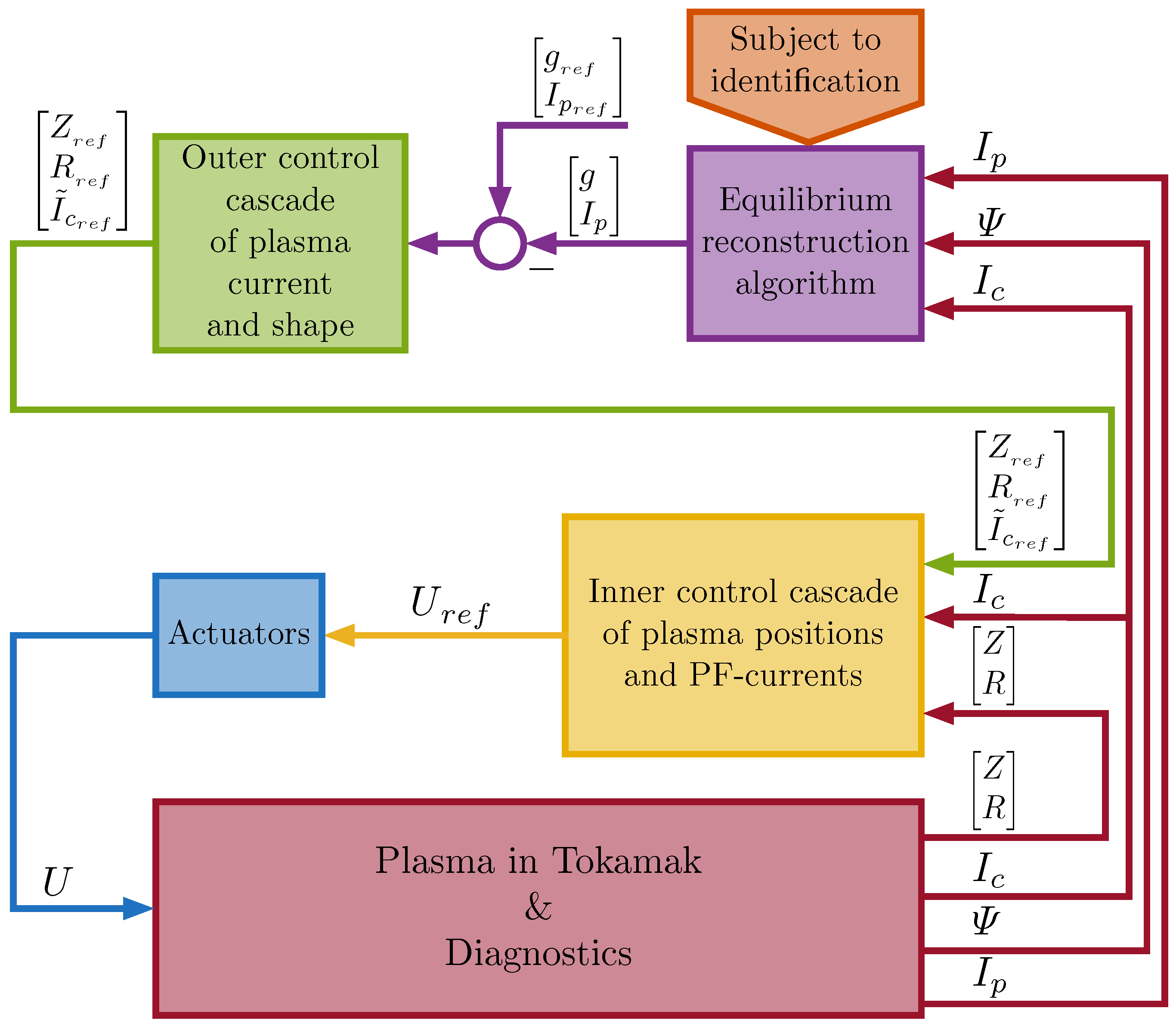
In any case, there is a critical point in this new identification approach. The point is that this approach greatly increases the response rate of plasma equilibrium reconstruction, but the estimation accuracy may not be as high as, for example, in the filaments (current rings) approach. So, the designer of the magnetic plasma control system should choose what is more adequate for the specific control problem since the plasma equilibrium reconstruction algorithm is included in the feedback (Figure 15).

12. Patents

The authors received the patent of the RF on the approach of modeling plasma magnetic control systems with the plasma equilibrium reconstruction algorithm in feedback #2702137 with the priority from 28 April 2017 [36]. The next application for the RF patent was submitted for the structure and approach of the digital testbed under the number 2021128495.

References

- Wesson, J. Tokamaks, 3rd ed.; Clarendon Press: Oxford, UK, 2004. [Google Scholar]
- Mitrishkin, Y.V.; Korostelev, A.Y.; Dokuka, V.N.; Khayrutdinov, R.R. Synthesis and simulation of a two-level magnetic control system for tokamak-reactor plasma. Plasma Phys. Rep. 2011, 37, 279–320. [Google Scholar] [CrossRef]
- Mitrishkin, Y. Upravleniye Plazmoi v Eksperimentalnikh Termoyadernikh Ustanovkakh: Adptivniye Avtokolebatelniye i Robustniye Sistemi Upravleniya [Plasma Control in Experimental Thermonuclear Installations: Adaptive Auto-Oscillation and Robust Control Systems]; KRASAND: Moscow, Russia, 2016. (In Russian) [Google Scholar]
- Mitrishkin, Y.; Kartsev, N.; Kuznetsov, E.; Korostelev, A. Metodi i Sistemi Magnitnogo Upravleniya Plazmoi v Tokamakakh [Methods and Systems of Plasma Magnetic Control in Tokamaks]; KRASAND: Moscow, Russia, 2020. (In Russian) [Google Scholar]
- Mitrishkin, Y.V.; Kartsev, N.M.; Zenkov, S.M. Stabilization of unstable vertical position of plasma in T-15 tokamak. I. Autom. Remote Control 2014, 75, 281–293. [Google Scholar] [CrossRef]
- Mitrishkin, Y.V.; Kartsev, N.M.; Zenkov, S.M. Stabilization of unstable vertical position of plasma in T-15 tokamak. II. Autom. Remote Control 2014, 75, 1565–1576. [Google Scholar] [CrossRef]
- Mitrishkin, Y.V.; Prokhorov, A.A.; Korenev, P.S.; Patrov, M.I. Plasma magnetic time-varying nonlinear robust control system for the Globus-M/M2 tokamak. Control Eng. Pract. 2020, 100, 104446. [Google Scholar] [CrossRef]
- Mitrishkin, Y.; Prokhorov, A.; Korenev, P.; Patrov, M. Hierarchical robust switching control method with the Improved Moving Filaments equilibrium reconstruction code in the feedback for tokamak plasma shape. Fusion Eng. Des. 2019, 138, 138–150. [Google Scholar] [CrossRef]
- Kuznetsov, E.A.; Mitrishkin, Y.V.; Kartsev, N.M. Current inverter as self-oscillating actuator in applications for plasma position control systems in the Globus-M/M2 and T-11M tokamaks. Fusion Eng. Des. 2019, 143, 247–258. [Google Scholar] [CrossRef]
- Mitrishkin, Y.; Korenev, P.; Konkov, A.; Kartsev, N.; Smirnov, I. New horizontal and vertical field coils with optimised location for robust decentralized plasma position control in the IGNITOR tokamak. Fusion Eng. Des. 2021. accepted. [Google Scholar]
- Hommen, G.; de Baar, M.; Nuij, P.; McArdle, G.; Akers, R.; Steinbuch, M. Optical boundary reconstruction of tokamak plasmas for feedback control of plasma position and shape. Rev. Sci. Instrum. 2010, 81, 113504. [Google Scholar] [CrossRef] [Green Version]
- Beghi, A.; Cenedese, A. Advances in real-time plasma boundary reconstruction: From gaps to snakes. IEEE Control Syst. Mag. 2005, 25, 44–64. [Google Scholar] [CrossRef]
- Lao, L.L.; St. John, H.; Stambaugh, R.D.; Kellman, A.G.; Pfeiffer, W. Reconstruction of current profile parameters and plasma shapes in tokamaks. Nucl. Fusion 1985, 25, 1611–1622. [Google Scholar] [CrossRef]
- Korenev, P.; Mitrishkin, Y.; Patrov, M. Rekonstrukciya ravnovesnogo raspredeleniya parametrov plazmy tokamaka po vneshnim magnitnym izmereniyam i postroenie lineinykh plazmennykh modelei [Reconstruction of equilibrium distribution of tokamak plasma parameters by external magnetic measurements and construction of linear plasma models]. Mechatronics Autom. Control 2016, 17, 254–265. (In Russian) [Google Scholar]
- Coda, S.; Ahn, J.; Albanese, R.; Alberti, S.; Alessi, E.; Allan, S.; Anand, H.; Anastassiou, G.; Andrèbe, Y.; Angioni, C.; et al. Overview of the TCV tokamak program: Scientific progress and facility upgrades. Nucl. Fusion 2017, 57, 102011. [Google Scholar] [CrossRef]
- Mitrishkin, Y.V. Plasma magnetic control systems in D-shaped tokamaks and imitation digital computer platform in real time for controlling plasma current and shape. Adv. Syst. Sci. Appl. 2021, 21, 1–14. [Google Scholar]
- Ariola, M.; Pironti, A. Magnetic Control of Tokamak Plasmas, 2nd ed.; Springer: Berlin, Germany, 2016. [Google Scholar]
- Lazarus, E.; Lister, J.; Neilson, G. Control of the vertical instability in tokamaks. Nucl. Fusion 1990, 30, 111–141. [Google Scholar] [CrossRef]
- Forsythe, G.; Malcolm, M.; Moler, C. Computer Methods for Mathematical Computations; Prentice Hall: Englewood Cliffs, NJ, USA, 1977. [Google Scholar]
- Duan, G.R.; Yu, H.H. LMIs in Control Systems; CRC Press: Boca Raton, FL, USA, 2013. [Google Scholar]
- Chilali, M.; Gahinet, P.; Apkarian, P. Robust pole placement in LMI regions. IEEE Trans. Autom. Control 1999, 44, 2257–2270. [Google Scholar] [CrossRef] [Green Version]
- Cybenko, G. Approximation by superpositions of a sigmoidal function. Math. Control Signals Syst. 1992, 5, 455. [Google Scholar] [CrossRef] [Green Version]
- Lister, J.B.; Schnurrenberger, H. Fast non-linear extraction of plasma equilibrium parameters using a neural network mapping. Nucl. Fusion 1991, 31, 1291. [Google Scholar] [CrossRef] [Green Version]
- Coccorese, E.; Morabito, C.; Martone, R. Identification of noncircular plasma equilibria using a neural network approach. Nucl. Fusion 1994, 34, 1349. [Google Scholar] [CrossRef]
- Windsor, C.G.; Todd, T.N.; Trotman, D.L.; Smith, M.E.U. Real-time electronic neural networks for iter-like multiparameter equilibrium reconstruction and control in compass-d. Fusion Technol. 1997, 32, 416–430. [Google Scholar] [CrossRef]
- Zhu, Z.J.; Guo, Y.; Yang, F.; Xiao, B.J.; Li, J.G. Estimation of plasma equilibrium parameters via a neural network approach. Chin. Phys. B 2019, 28, 125204. [Google Scholar] [CrossRef]
- Sutskever, I.; Vinyals, O.; Le, Q.V. Sequence to sequence learning with neural networks. In Advances in Neural Information Processing Systems; MIT Press: Cambridge, MA, USA, 2014; pp. 3104–3112. [Google Scholar]
- Rosenblatt, F. The perceptron: A probabilistic model for information storage and organization in the brain. Psychol. Rev. 1958, 65, 386. [Google Scholar] [CrossRef] [Green Version]
- Kingma, D.P.; Ba, J. Adam: A method for stochastic optimization. arXiv 2014, arXiv:1412.6980. [Google Scholar]
- Chung, J.; Gulcehre, C.; Cho, K.; Bengio, Y. Empirical evaluation of gated recurrent neural networks on sequence modeling. arXiv 2014, arXiv:1412.3555. [Google Scholar]
- Singh, M.; Fuenmayor, E.; Hinchy, E.P.; Qiao, Y.; Murray, N.; Devine, D. Digital Twin: Origin to future. Appl. Syst. Innov. 2021, 4, 36. [Google Scholar] [CrossRef]
- Kritzinger, W.; Karner, M.; Traar, G.; Henjes, J.; Sihn, W. Digital Twin in manufacturing: A categorical literature review and classification. IFAC-PapersOnLine 2018, 51, 1016–1022. [Google Scholar] [CrossRef]
- Mitrishkin, Y.; Kartsev, N.; Prokhorov, A.; Pavlova, E.; Korenev, P.; Konkov, A.; Kruzhkov, V.; Ivanova, S. Tokamak plasma models development for plasma magnetic control systems design by first principle equations and identification approach. Procedia Comput. Sci. 2021, 186, 466–474. [Google Scholar] [CrossRef]
- Shalev-Shwartz, S.; Ben-David, S. Understanding Machine Learning: From Theory to Algorithms; Cambridge University Press: New York, NY, USA, 2013. [Google Scholar] [CrossRef]
- Parrott, A.; Warshaw, L. Industry 4.0 and the Digital Twin: Manufacturing Meets Its Match; Deloitte University Press: New York, NY, USA, 2017. [Google Scholar]
- Mitrishkin, Y.; Prohorov, A.; Korenev, P.; Patrov, M. Sposob Formirovfniya Modeli Magnitnogo Upravleniya Formoy i Tokom Plasmi s Obratnoy Svyazyu v Tokamake. [Method of Formation of the Model of Magnetic Control of Plasma Shape and Current with Feedback in a Tokamak]. Patent for Invention of the Russian Federation No. 2702137, 28 April 2017. (In Russian). [Google Scholar]
Figure 1.
Vertically elongated tokamak without iron core: 1 is the VV; 2 is the toroidal field coil; 3 are the poloidal field inner and outer coils; 4 are plasma and helical magnetic lines (©ITER Project Center (Russia):
https://www.iterrf.ru/index.php/istoriya-sozdaniya-proekta, accessed on 21 December 2021).
Figure 2.
Structure scheme of the plasma position, current and shape control system of Globus-M2 tokamak.
Figure 3.
Globus-M2 tokamak (©Ioffe Physics and Technology Institute of RAS, St. Petersburg, Russia).
Figure 4.
Poloidal system of the Globus-M2 tokamak and plasma boundary with strike points , and gaps –.
Figure 5.
Robust observer synthesized via LMIs for use in a real experiment. The red vector signal includes experimental signals obtained by the magnetic diagnostic system. The blue vector signal includes voltages on the poloidal coils. The yellow signal contains states estimation, which includes gaps estimation.
Figure 6.
Comparison of gaps variations derived by LPV model obtained from the FCDI code (blue line) and estimation of gap variations obtained from robust observer synthesized by LMIs (red line). Globus-M2 discharge .
Figure 7.
Estimation of the gap values in the discharge #37712 of the Globus-M2 spherical tokamak.
Figure 8.
Multilayer perceptron.
Figure 10.
Divertor phase of the test discharge #37270.
Figure 11.
Encoder–decoder model.
Figure 12.
Neural network estimation of the gap values. Discharge #37270 of the Globus-M2 spherical tokamak.
Figure 13.
Digital twin containing a real dynamical plant with real feedback controller and virtual dynamical plant with a real feedback controller closed by the feedback of information flows: real-time data and algorithms, commands, adaptations, and recommendations.
Figure 14.
Real-time test bed for plasma control in tokamaks. The test bed consists of two Speedgoat performance real-time target machines that are connected in feedback: one computer plays the role of the controlled plant model and the other one is the MIMO controller (
https://www.ipu.ru/press-center/62866, accessed on 21 December 2021).
Figure 15.
Scheme of digital twin of Globus-M2. The block with plasma equilibrium reconstruction algorithm is marked by red color.
Figure 16.
Real-time simulation of gaps variations derived by LPV model obtained from the FCDI code (blue line) and estimation of gap variations obtained from robust observer synthesized by LMIs (red line). Discharge .
Figure 17.
Real-time simulation of gaps g derived by LTI model obtained from the FCDI code (blue line) and estimation of gaps obtained from static matrix (red line). Discharge .