Numerical Simulation of Cubic-Quartic Optical Solitons with Perturbed Fokas–Lenells Equation Using Improved Adomian Decomposition Algorithm

Abstract

The current manuscript displays elegant numerical results for cubic-quartic optical solitons associated with the perturbed Fokas–Lenells equations. To do so, we devise a generalized iterative method for the model using the improved Adomian decomposition method (ADM) and further seek validation from certain well-known results in the literature. As proven, the proposed scheme is efficient and possess a high level of accuracy.

1. Introduction

Optical solitons, which emerge from nonlinear evolution equations, have been studied for the past few decades. The self-phase modulation (SPM) that comes from intensity-dependent refractive index of light coupled with the chromatic dispersion (CD) leads to a delicate balance, which sustains the solitons that travel down the fiber for intercontinental distances. Several models that give way to optical solitons are addressed in Mathematics, Physics and telecommunications engineering. The notion of cubic-quartic (CQ) solitons surfaced in the realm of nonlinear fiber optics for the first time in 2017, and an avalanche of results were eventually visible. Prior to this, it is the concept of pure-quartic solitons that was visible [1]. Such CQ solitons were introduced due to the sheer necessity whenever CD is low enough to be ignored and thus third-order dispersion (3OD) and fourth-order dispersion (4OD) effects are able to compensate for this depletion. This allows the sustainment of the necessary balance between the dispersion effects and SPM to be restored, allowing stable solitons to be transmitted across intercontinental distances.

Furthermore, optical solitons have painstakingly fashioned pulse transmission technology for several waveguides [2,3,4]. This technical feat is described at a spectacular level by several mathematical models. The Fokas–Lenells equation (FLE), which governs this dynamic, was originally launched almost a decade ago [5,6,7]. Since its initial introduction, this model has garnered widespread recognition in the fiber-optics community. In the past, several types of soliton solutions for this model were recovered. However, none of these studies have explored the implications of perturbation terms that emerge as a result of natural factors in soliton transmission dynamics. The FLE is examined in this study, along with a few perturbative effects.

As all previous efforts on CQ solitons have been analytical in nature, it is therefore imperative to consider such solitons from a numerical standpoint. Thus, this article employs a numerical approach to CQ solitons. However, the methodology used to present the findings in this manuscript is the enhanced form of the strongly reliant Adomian’s method called the improved Adomian decomposition method (ADM) [8]. We will, therefore, suggest an efficient numerical scheme for solving CQ optical solitons associated with the perturbed FLE. The approach will be based on the improved ADM. Besides, improved ADM is a fast numerical approach for integral and functional solutions that is based on Adomian’s method [9]. Validation of the suggested method will be carried out with recent analytical results in the literature. The integration method reveals promising results without the need of either linearization or any artificial boundary condition. Lastly, the improved ADM architecture has its shortcomings. It fails to capture the effect of soliton radiation that is a major detrimental factor in the soliton propagation.

The manuscript is arranged in the following manner: the perturbed FLE is described in Section 2; while the governing model is addressed via the improved ADM in Section 3. The simulated numerical results are retrieved in Section 4, and some concluding comments are reported in Section 5.

2. Governing Model

The dimensionless form of the CQ solitons with the perturbed FLE is indicated below [10]

$$i{q}_t+ia{q}_{xxx}+b{q}_{xxxx}+{\left|q\right|}^2\left(cq+id{q}_x\right)=i\left[\alpha q_x+\lambda {\left({\left|q\right|}^{2}q\right)}_x+\mu {\left({\left|q\right|}^2\right)}_{x}q\right],$$

(1)

where $x$ and $t$ are the independent spatial and temporal variables, sequentially; while the function $q=q\left(x,t\right)$ is the complex wave profile. Additionally, starting with the left-hand side, the first component indicates the temporal evolution, whereas $a$ and $b$ are the coefficients of the 3OD and 4OD, sequentially; while d gives the nonlinear dispersion term and the coefficient c is the Kerr law nonlinearity. Additionally for Equation (1), λ is the self-steepening term, whereas the coefficients μ and α are for the higher-order and inter-modal dispersions, sequentially.

3. Analysis of the Method

This section introduces the efficient improved ADM to derive a numerical scheme for the CQ–FLE given in Equation (1). Initially, we offer the fundamental technique for constructing nonlinear wave solutions of the equation. In our analysis, the complex CQ–FLE given in Equation (1) will be converted to a real system using

$$q\left(x,t\right)=u_1+i{u}_2.$$

(2)

Plugging Equation (2) into Equation (1), we have

$$\begin{array}{c}i{\left(u_1+i{u}_2\right)}_t+ia{\left(u_1+i{u}_2\right)}_{xxx}+b{\left(u_1+i{u}_2\right)}_{xxxx}\\ +{\left|u_1+i{u}_2\right|}^2\left(c\left(u_1+i{u}_2\right)+id{\left(u_1+i{u}_2\right)}_x\right)=i[\alpha {\left(u_1+i{u}_2\right)}_x\\ +\lambda {\left({\left|q{u}_1+i{u}_2\right|}^2\left(u_1+i{u}_2\right)\right)}_x+\mu {\left({\left|u_1+i{u}_2\right|}^2\right)}_x\left(u_1+i{u}_2\right)].\end{array}$$

(3)

Thus, from the above equation, the following system is obtained, after splitting the real and imaginary parts as follows

$$\begin{array}{c}{u}_{1t}+a{u}_{1xxx}+b{u}_{2xxxx}+\left(u_1^2+u_2^2\right)\left(c{u}_2+d{u}_{1x}\right)\\ =\alpha u_{1x}+\lambda {\left(\left(q^2{u}_1^2+u_2^2\right)u_2\right)}_x+\mu {\left(u_1^2+u_2^2\right)}_x{u}_2,\end{array}$$

(4)

and

$$\begin{array}{c}-u_{2t}-a{u}_{2xxx}+b{u}_{1xxxx}+\left(u_1^2+u_2^2\right)\left(c{u}_1-d{u}_{2x}\right)\\ =-\alpha u_{2x}+\lambda {\left(\left(q^2{u}_1^2+u_2^2\right)u_1\right)}_x+\mu {\left(u_1^2+u_2^2\right)}_x{u}_1,\end{array}$$

(5)

where

$$u_1\left(x,0\right)={\left[q\left(x,0\right)\right]}_R,$$

and

$$u_2\left(x,0\right)={\left[q\left(x,0\right)\right]}_I.$$

Now, on using the Adomian’s approach, the solution of the above system transforms into the following infinite series

$$u_1\left(x,t\right)={\displaystyle \sum }_{n=0}^{\infty }{u}_{1n}\left(x,t\right),$$

(6)

and

$$u_2\left(x,t\right)={\displaystyle \sum }_{n=0}^{\infty }{u}_{2n}\left(x,t\right).$$

(7)

Here $u_{1n},u_{2n},n\ge 0,$ will be obtained recurrently. Furthermore, in an operator form, we re-express Equations (4) and (5) as follows

$$\begin{array}{c}{L}_t\left(u_1\right)+a{u}_{1xxx}+b{u}_{2xxxx}+\left(u_1^2+u_2^2\right)\left(c{u}_2+d{u}_{1x}\right)\\ =\alpha u_{1x}+\lambda {\left(\left(q^2{u}_1^2+u_2^2\right)u_2\right)}_x+\mu {\left(u_1^2+u_2^2\right)}_x{u}_2,\end{array}$$

(8)

and

$$\begin{array}{c}{L}_t\left(u_2\right)+a{u}_{2xxx}-b{u}_{1xxxx}-\left(u_1^2+u_2^2\right)\left(c{u}_1-d{u}_{2x}\right)\\ =\alpha u_{2x}-\lambda {\left(\left(q^2{u}_1^2+u_2^2\right)u_1\right)}_x-\mu {\left(u_1^2+u_2^2\right)}_x{u}_1,\end{array}$$

(9)

where

$$L_t=\frac{\partial }{\partial t}.$$

Further, using the inverse operator $L_t^{-1}$ on both sides of Equations (8) and (9) yields

$$\begin{array}{c}{u}_1\left(x,t\right)=u_1\left(x,0\right)-L_t^{-1}a{u}_{1xxx}-L_t^{-1}b{u}_{2xxxx}-L_t^{-1}\left(u_1^2+u_2^2\right)\left(c{u}_2+d{u}_{1x}\right)\\ +L_t^{-1}\alpha u_{1x}+\lambda {\left(\left(q^2{u}_1^2+u_2^2\right)u_2\right)}_x+L_t^{-1}\mu {\left(u_1^2+u_2^2\right)}_x{u}_2,\end{array}$$

and

$$\begin{array}{c}{u}_2\left(x,t\right)=u_2\left(x,0\right)-L_t^{-1}a{u}_{2xxx}+L_t^{-1}b{u}_{1xxxx}+L_t^{-1}\left(u_1^2+u_2^2\right)\left(c{u}_1-d{u}_{2x}\right)\\ +L_t^{-1}\alpha u_{2x}-L_t^{-1}\lambda {\left(\left(q^2{u}_1^2+u_2^2\right)u_1\right)}_x-L_t^{-1}\mu {\left(u_1^2+u_2^2\right)}_x{u}_1.\end{array}$$

Next, re-expressing the above system via the Adomian polynomials, we have

$$u_1\left(x,t\right)=u_1\left(x,0\right)-L_t^{-1}a{u}_{1xxx}+L_t^{-1}b{u}_{2xxxx}+L_t^{-1}\alpha u_{1x}+L_t^{-1}{A}_1,$$

(10)

and

$$u_2\left(x,t\right)=u_2\left(x,0\right)-L_t^{-1}a{u}_{2xxx}-L_t^{-1}b{u}_{1xxxx}+L_t^{-1}\alpha u_{2x}+L_t^{-1}{A}_2,$$

(11)

where the terms $A_1$ and $A_2$ in Equations (10) and (11) are the nonlinear terms represented by

$$A_1=-\left(u_1^2+u_2^2\right)\left(c{u}_2+d{u}_{1x}\right)+\lambda {\left(\left(q^2{u}_1^2+u_2^2\right)u_2\right)}_x+\mu {\left(u_1^2+u_2^2\right)}_x{u}_2,$$

(12)

and

$$A_2=\left(u_1^2+u_2^2\right)\left(c{u}_1-d{u}_{2x}\right)-\lambda {\left(\left(q^2{u}_1^2+u_2^2\right)u_1\right)}_x-\mu {\left(u_1^2+u_2^2\right)}_x{u}_1,$$

(13)

Of which $A_1={{\displaystyle \sum }}_{n=0}^{\infty }{A}_{1n}$ and $A_2={{\displaystyle \sum }}_{n=0}^{\infty }{A}_{2n}$, where $A_{1n},\dots ,A_{2n},\dots$ are the Adomian polynomials, which may be generated from all types of nonlinearity, using Adomian’s specific algorithms. Plugging the solution forms in Equations (5) and (6), as well as $A_1$ and $A_2$ in Equations (12) and (13), into Equations (10) and (11) yields

$$\begin{array}{c}{{\displaystyle \sum }}_{n=0}^{\infty }{u}_{1n}\left(x,t\right)=u_1\left(x,0\right)-L_t^{-1}a{{\displaystyle \sum }}_{n=0}^{\infty }{(u_{1n}\left(x,t\right))}_{xxx}\\ +L_t^{-1}b{{\displaystyle \sum }}_{n=0}^{\infty }{(u_{2n}\left(x,t\right))}_{xxxx}+L_t^{-1}{{\displaystyle \sum }}_{n=0}^{\infty }{A}_{1n},\end{array}$$

(14)

and

$$\begin{array}{c}{\displaystyle {\displaystyle \sum }_{n=0}^{\infty }}{u}_{2n}\left(x,t\right)=u_2\left(x,0\right)-L_t^{-1}a{\displaystyle {\displaystyle \sum }_{n=0}^{\infty }}{(u_{2n}\left(x,t\right))}_{xxx}\\ +L_t^{-1}b{\displaystyle {\displaystyle \sum }_{n=0}^{\infty }}{(u_{1n}\left(x,t\right))}_{xxxx}+L_t^{-1}{\displaystyle {\displaystyle \sum }_{n=0}^{\infty }}{A}_{2n}.\end{array}$$

(15)

The following recursive relations are introduced as a result of the decomposition analysis

$$u_{1,0}\left(x,t\right)=u_1\left(x,0\right),$$

(16)

$$u_{2,0}\left(x,t\right)=u_2\left(x,0\right),$$

(17)

$$\begin{array}{c}{u}_{1,k+1}\left(x,t\right)=-L_t^{-1}a{{\displaystyle \sum }}_{n=0}^{\infty }{(u_{1n}\left(x,t\right))}_{xxx}\\ +L_t^{-1}b{{\displaystyle \sum }}_{n=0}^{\infty }{(u_{2n}\left(x,t\right))}_{xxxx}+L_t^{-1}{{\displaystyle \sum }}_{n=0}^{A_{1n}}{A}_{1n},\end{array}$$

(18)

and

$$\begin{array}{c}{u}_{2,k+1}\left(x,t\right)=-L_t^{-1}a{{\displaystyle \sum }}_{n=0}^{\infty }{(u_{2n}\left(x,t\right))}_{xxx}\\ +L_t^{-1}b{{\displaystyle \sum }}_{n=0}^{\infty }{(u_{1n}\left(x,t\right))}_{xxxx}+L_t^{-1}{{\displaystyle \sum }}_{n=0}^{\infty }{A}_{2n}.\end{array}$$

(19)

Thus, we determine $u_1$ and $u_2$ as follows

$$u_1=u_{1,0}+u_{1,1}+u_{1,2}+\dots ,$$

and

$$u_2=u_{2,0}+u_{2,1}+u_{2,2}+\dots ,$$

and the entire approximate solution for Equation (1) is derived by plugging the preceding equations into Equation (2), which is connected to Equations (16)–(19) to yield the following

$$q\left(x,t\right)=u_{1,0}+u_{1,1}+u_{1,2}+\cdots +i\left(u_{2,0}+u_{2,1}+u_{2,2}+\cdots \right).$$

(20)

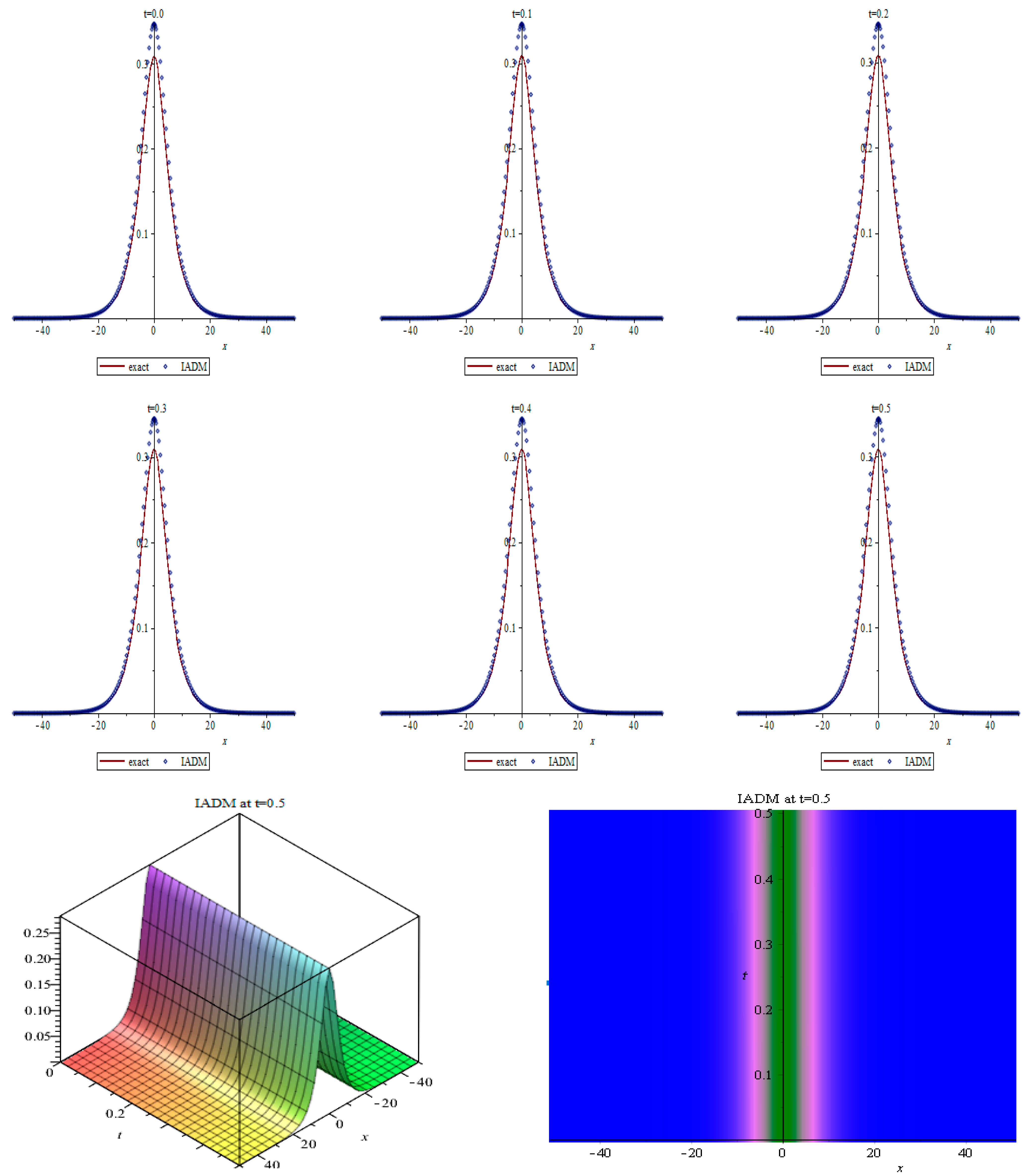
4. Numerical Results

This section analyzes three distinct scenarios for the CQ–FLE given in Equation (1) to demonstrate how the improved ADM scheme derived in the previous Section might be applied. We analyze the CQ bright soliton of the perturbed FLE, which was recently derived by Elsayed et al. [10] that is formulated as

$$q\left(x,t\right)=A\sec \mathrm{h}\left[B\left(x–vt\right)\right]e^{i\left(-k_{l}x+{\omega }_{l}t+\mathsf{\theta }\right)},$$

(21)

where A and B are the soliton’s amplitude and width, sequentially, that are structured as

$$A=\pm \frac{{\Delta }_0}{10}\sqrt{-\frac{30}{{\Delta }_1}},$$

(22)

and

$$B=\frac{1}{2}\sqrt{-\frac{{\Delta }_0}{5}},$$

(23)

along with

$$v=-\alpha -3a{k}^2+4b{k}^3,$$

$${\Delta }_0=\frac{1}{b}\left(3ak-6b{k}^2\right),$$

and

$${\Delta }_3=\frac{1}{b}\left(c+dk+\lambda k\right).$$

Moreover, from Equations (22)–(23), the constraint criteria for the possibility of bright solitons were given by

$${\Delta }_0<0,{\Delta }_3<0.$$

The phase component in Equation (21) represents the soliton’s velocity. $\theta$ is the phase constant. The soliton’s frequency is

$$k=-\frac{a}{4b},$$

while the wave number is

$$\omega =-\frac{k\left(36k{a}^2-119ab{k}^2+119b^2{k}^3+25b\alpha \right)}{25b}.$$

Consider the CQ-FLE (1) along with the parameters [10]

$$\alpha =0.1,\lambda =1,\mu =1,d=3\lambda +2\mu .$$

In addition, the initial condition at $t$ = 0 from Equation (21) follows as

$$q\left(x,0\right)=A\sec \mathrm{h}\left[B\left(x\right)\right]e^{i\left(-kx+\mathsf{\theta }\right)}.$$

(24)

However, for the sake of numerical simulation, we consider the following three cases of the model fixed parameters:

Case 1:

$$a=0.5,b=-1,c=1.$$

Case 2:

$$a=1,b=-2,c=2.$$

Case 3:

$$a=0.5,b=-0.5,c=1.$$

In what follows, we report the absolute error differences between the exact solution and that of the approximate solution using the improved ADM of the three solution cases in

Table 1. Absolute error for Case 1 for x = 20, x = 50.

t	Error When x = 20	Error When x = 50
0.0	0.00304922317	0.0000878266951
0.1	0.00306667344	0.0000883416821
0.2	0.00308409727	0.0000888560318
0.3	0.00310149460	0.0000893697436
0.4	0.00311886552	0.0000898828190
0.5	0.00313621000	0.0000903952578

,

Table 2. Absolute error for Case 2 for x = 20, x = 50.

t	Error When x = 20	Error When x = 50
0.0	0.00692281558	0.0001996291264
0.1	0.00692913128	0.0001998464016
0.2	0.00693539773	0.0002000633452
0.3	0.00694161507	0.0002002799558
0.4	0.00694778339	0.0002004962310
0.5	0.00695390283	0.0002007121745

and

Table 3. Absolute error for Case 3 for x = 20, x = 50.

t	Error When x = 20	Error When x = 50
0.0	0.000574951108	4.67316035 × 10−7
0.1	0.000570769757	4.63918739 × 10−7
0.2	0.000566597435	4.60529257 × 10−7
0.3	0.000562434066	4.57147514 × 10−7
0.4	0.000558279554	4.5377342 × 10−7
0.5	0.000554133811	4.50406915 × 10−7

. Furthermore, we portray the respective solution cases in Figure 1, Figure 2 and Figure 3 for various values of $t$ over the interval −50 ≤ x ≤ 50. Without loss of generality, these figures are self-explanatory, as the proposed numerical method performs excellently. Additionally, an absolute agreement is noted in these figures in the bulk parts of the bell-shaped solution; only a small disparity is noted at the peak of the curves. This disparity can equally be overcome when the model’s parameters are suitably chosen and, also by considering more iterates/approximants in the series summation.

5. Conclusions

In conclusion, CQ optical solitons are a modern topic of great interest in the field of optical communications. In this paper, the effect of changing the optical parameters of such CQ solitons with perturbed FLE was studied.

The unperturbed FLE, coupled with the chromatic dispersion and spatiotemporal dispersion has been studied for the past few decades [5,6,7]. The initial-boundary value problems, that are referred to as the linearizable boundary conditions, for the FLE are analyzed in [5]. A class of exact combined solitary wave solutions of the FLE is constructed by adopting the complex envelope function ansatz [6]. The influences of spatiotemporal dispersion on the characteristics of combined solitary waves are also discussed in [6]. A class of chirped soliton-like solutions including bright, dark and kink solitons is derived in [8]. The associated chirp, including linear and nonlinear contributions, is also determined for each of optical pulses in [7]. When compared with [5,6,7], none of these studies have explored the implications of perturbation terms that emerge as a result of natural factors in soliton transmission dynamics. Therefore, the FLE is examined in this study along with a few perturbative effects that are crucial to many applications in photonics, performing essential functions in lasing, frequency conversion, and entangled-photon generation. Furthermore, these perturbative effects may be used to generate new frequency components from high power pulses, resulting in optical pulses with spectral widths much larger than the gain-bandwidth of optical fiber amplifiers. In other words, these nonlinear effects can be used to make useful devices capable of processing high-speed optical signals. Additionally, none of the works in [5,6,7] have addressed the implications of cubic-quartic solitons. Thus, the current paper reports cubic-quartic solitons that are the sheer necessity whenever CD is low enough to be ignored. As a result, CQ solitons compensate for this depletion. Hence, CQ solitons allow the sustainment of the necessary balance between the dispersion effects and self-phase modulation to be restored, allowing stable solitons to be transmitted across intercontinental distances. The results of the current paper are new and are elegant numerical results for cubic-quartic optical solitons associated with the perturbed FLE, where the perturbation terms are all of Hamiltonian type and the chromatic dispersion is replaced by a combination of third-order dispersion and fourth-order dispersion.

Cubic-quartic solitons with the perturbed FLE (1) have been addressed for the analytical study and revealed quite a number of interesting solitons in nonlinear optics [10], where bright and singular solitons have been yielded by a couple of integration approaches. While all previous efforts on CQ solitons have been analytical in nature [10], it is therefore imperative to consider such solitons from a numerical standpoint. Thus, the current paper focuses on the integrability of the perturbed FLE (1) for the numerical investigation using the improved ADM architecture for the very first time. Analytical solutions are possible using simplifying assumptions that may not realistically reflect reality. In many applications, analytical solutions are impossible to achieve. Hence, numerical methods make it possible to obtain realistic solutions without the need for simplifying assumptions. The improved ADM adopted in this paper leads to the emergence of bright soliton solutions and is being reported for the first time in this paper, which makes these results novel. The bright soliton solutions are very important, and these soliton solutions are used to sustain pulse transmission through optical fibers in the telecommunications industry.

A promising technique called the improved ADM, which was based on the famous Adomian’s method, was utilized to derive a recurrent numerical scheme for the governing model and, furthermore, was successfully applied to the model through bright soliton solutions. The integration method firstly converts a special case of the complex-valued system into a real-valued system. Next, the integration scheme decomposes the solutions into infinite sums of components called infinite series. When compared with the famous Adomian’s method, the improved ADM reveals promising results without the need of either linearization or any artificial boundary condition. The scheme is indeed reliable as it was discovered to display results with higher accuracy. The numerical computations are simpler and faster than most of the traditional techniques. Finally, the method is recommended to investigate additional evolution equations.

References

1. Blanco-Redondo, A.; Sterke, C.M.D.; Sipe, J.E.; Krauss, T.F.; Eggleton, B.J.; Husko, C. Pure–quartic solitons. Nat. Commun. 2016, 7, 11048. [Google Scholar] [CrossRef] [PubMed] [Green Version]
2. Boutabba, N. Kerr-effect analysis in a three-level negative index material under magneto cross-coupling. J. Opt. 2018, 20, 025102. [Google Scholar] [CrossRef]
3. Eleuch, H.; Elser, D.; Bennaceur, R. Soliton propagation in an absorbing three-level atomic system. Laser Phys. Lett. 2004, 1, 391. [Google Scholar] [CrossRef]
4. Boutabba, N.; Eleuch, H.; Bouchriha, H. Thermal bath effect on soliton propagation in three-level atomic system. Synth. Met. 2009, 159, 1239–1243. [Google Scholar] [CrossRef]
5. Lennels, J.; Fokas, A.S. An integrable generalization of the nonlinear Schrödinger equation on the half-line and solitons. Inverse Probl. 2009, 25, 115006. [Google Scholar] [CrossRef]
6. Triki, H.; Wazwaz, A.M. Combined optical solitary waves of the Fokas–Lenells equation. Waves Rand. Complex Media 2017, 27, 587–593. [Google Scholar] [CrossRef]
7. Triki, H.; Wazwaz, A.M. New types of chirped soliton solutions for the Fokas–Lenells equation. Int. J. Numer. Methods Heat Fluid Flow 2017, 27, 1596–1601. [Google Scholar] [CrossRef]
8. Bakodah, H.O.; Banaja, M.A.; Alshaery, A.A.; Al Qarni, A.A. Numerical Solution of Dispersive Optical Solitons with Schrödinger-Hirota Equation by Improved Adomian Decomposition Method. Math. Probl. Eng. 2019, 2019, 2960912. [Google Scholar] [CrossRef] [Green Version]
9. Adomian, G. Solution of physical problems by decomposition. Comput. Math. Appl. 1994, 27, 145–154. [Google Scholar] [CrossRef] [Green Version]
10. Zayed, E.M.E.; Alngar, M.E.M.; Biswas, A.; Yıldırım, Y.; Khan, S.; Alzahrani, A.K.; Belic, M.R. Cubic–quartic optical soliton perturbation in polarization-preserving fibers with Fokas–Lenells equation. Optik 2021, 234, 166543. [Google Scholar] [CrossRef]
Figure 1. Comparison of the exact and improved ADM solutions for case 1 for −50 ≤ x ≤ 50.
Mathematics 10 00138 g001
Figure 2. Comparison of the exact and improved ADM solutions for case 2 for −50 ≤ x ≤ 50.
Mathematics 10 00138 g002
Figure 3. Comparison of the exact and improved ADM solutions for case 3 for −50 ≤ x ≤ 50.
Mathematics 10 00138 g003