Article

Mathematical Modeling and Associated Numerical Simulation of Fusion/Solidification Front Evolution in the Context of Severe Accident of Nuclear Power Engineering

1
Institut de Mathématiques de Bordeaux, University of Bordeaux, CNRS, UMR 5251, 33400 Talence, France
2
CEA-DES-IRESNE-DTN, CEA Cadarache, 13108 Saint Paul-lez-Durance, France
3
CEA-DES, Université Paris—Saclay, 91191 Gif-sur-Yvette, France
*
Author to whom correspondence should be addressed.
Mathematics 2022, 10(1), 116; https://doi.org/10.3390/math10010116
Submission received: 28 November 2021 / Revised: 22 December 2021 / Accepted: 24 December 2021 / Published: 31 December 2021
(This article belongs to the Special Issue Modeling and Numerical Analysis of Energy and Environment 2021)

Abstract

:
Considering transient processes where liquid/solid phase change occurs, this paper focuses on the associated modeling and numerical treatment in the frame of “Computational Fluid Dynamics” simulations. While being of importance in many industrial applications involving solidification and melting of mixed materials, including power and manufacturing engineering, the first application of this work pertains to the analysis of severe accidents in a nuclear reactor. Indeed, in this context, the molten core materials (a.k.a. corium) can form a high-temperature multiphase liquid pool at the boundary of which fusion and solidification phenomena are of prime importance. In this context, even if materials at play are treated as pure components, it is mandatory to distinguish two different phase change temperatures with a solid fusion temperature and a liquid solidification temperature. Accordingly, in the frame of a sharp interface representation, the paper introduces non-classical heterogeneous conditions at the liquid/solid boundary in such a way that both moving interface (through Stefan conditions associated with fusion or solidification) and static interface (imposing heat flux continuity) are supported at the same time on different spatial locations along this boundary. Within a monolithic resolution of Navier–Stokes and heat conduction equations, this interface is explicitly tracked with combined Front-Tracking and VOF methods. In order to ensure zero velocity in the solid phase, an Immersed Boundary Method and a direct forcing penalization are also introduced. The main relevant features of this combination of numerical methods are discussed along with their implementation in the TrioCFD code taking advantage of the pre-existing code capabilities. Numerical simulations including both verification tests and a case of interest for our industrial application are reported and demonstrate the applicability of the proposed triptych model+methods+code to treat such problems. The numerical tools and the simulation code developed in this work could be used not only in the several accident context but also to simulate melting, solidification and fusion processes occurring in aerodynamics, hypersonic reentry vehicles and laser applications to cite but a few.

1. Context and Introduction

A vast amount of physical processes involve solidification and melting of mixed materials, including power and manufacturing engineering. For instance, in the context of nuclear power engineering, melting processes are of prime interest during a severe accident progression as a consequence of the insufficient nuclear reactor core cooling. While not restricted to this context, we shall nonetheless employ it as a toy context for our subsequent developments.
Such ‘phase change’, from solid to liquid and vice-versa, implies drastic thermo-mechanical and chemical modifications of the materials under scrutiny. The transition area, also referred to as the ‘interface’, is of paramount importance for the appropriate description of such rapid modifications. In this work, we ought to improve the mathematical modeling and numerical simulations of such phase changes. The general physical model involves an incompressible hot liquid and a solid material exchanging mass and heat through their common interface. The motion of this interface is determined by these phase changes, i.e., the melting of the solid or the solidification of the liquid. Meanwhile, the phase changes are induced by the temperature gradients with respect to the material characteristics. The temperature gradients are modified by the liquid convection, the cooling/heating from the external world, and the transfer of mass and heat during the phase changes. The corresponding mathematical modeling must involve those coupled effects. As a consequence, the model must pay a special attention at capturing and tracking the interface region in-between the liquid and solid phases, and the different materials involved. Moreover, in the context of nuclear reactor core meltdown, the material under consideration is the so-called ‘corium’, a complex mixture of nuclear fuel, fission products, control rods, structural materials of the reactor, products of their chemical reaction with air, water and steam, etc. This liquid corium is generally contained within a metallic container or vessel, the integrity of which is to be ensured. The liquid corium pool in contact with the cold vessel can solidify, creating a protective ‘solid corium crust’ in-between the vessel and the liquid. On the contrary, large convection phenomena or new material addition may also change the thermal condition in contact with the crust which may melt back into the corium liquid, removing, as such, the thermal protection of the vessel. The determination of the transient conditions, in order to maintain the integrity of the container, must resort mainly to numerical simulation because such extreme situations are difficult to reproduce experimentally at large scale. As such, an appropriate physical model supplemented with robust and efficient numerical simulation tools are needed.
The simplified model of Partial Differential Equations (PDEs) under consideration involves a conducting domain (liquid and solid phases and the container) and the incompressible liquid phase coupled through a moving interface between the liquid and solid phases The conduction in the domain is solved by the heat equation subject to thermal boundary conditions on a fixed grid relying on a Ghost Fluid method [1]. The liquid phase is modeled by the incompressible Navier–Stokes equations subject to gravity within a closed solid pool with only one open boundary on the top, from which, new material can be supplemented. The Navier–Stokes equations are solved by a projection/correction method on a fixed staggered Cartesian mesh [2,3] on the whole domain. The interface is the location where the phase changes may occur, i.e., solidification of the liquid or fusion of the solid. In our context, this moving phase boundary problem reduces to the well known Stefan problem [4]. In the Stefan problem, the moving phases interface and the associated conditions are non-linear functions of the unknown location of the interface changing in time. The source of non-linearity lies in the phase change itself, and, the temperature dependent properties of the material. Moreover the solids are considered as motionless, and, they only can gain or loose mass and energy during the phase changes.
In this work, an explicit tracking of this sharp interface is considered. Indeed, in our case of application, this interface remains continuous as the phase change does not involve complicated phase configurations (e.g., with a dispersed phase embedded in a continuous one), in such a way that a front tracking type modeling [5] is readily applicable. In the frame of multiphase corium simulation, this choice is to be distinguished from:
  • an enthalpy-based numerical method [6] that is the most common approach reported in the literature for simulating the solidification at the interface of an homogeneous liquid corium pool (see, for instance, [7]). The work reported in this paper aims at providing an alternative and a priori more accurate approach with an explicit tracking of such a liquid/solid interface;
  • the diffuse interface approach followed in [8] where liquid phase stratification involving droplet detachment and coalescence processes in a two-phase corium pool is simulated. This work and the current one are complementary as they pursue the same goal: providing models and numerical methods for simulating the thermalhydraulic behaviour of a corium pool composed of different chemically reactive liquid phases with, possibly, liquid/solid phase change at their boundaries.
This paper focuses on several important characteristics of the numerical methods at play that are related to important features of corium pool simulation. First of all, the complexity of the corium mixture in terms of phase segregation for a multicomponent materials requires, in principle, evolution equations for the phase composition so that, phase thermophysical properties can be evaluated based on the local composition. At this stage of our R&D effort, in the restricted framework of a single liquid and a single solid phase, a simplified assumption is considered where both liquid and solid materials are treated as pure materials with different (but fixed in time) properties. As such, contrarily to the classical Stefan problem, two different phase change temperatures need to be defined: a solidification (resp. fusion) temperature T sol (resp. T fus ) for the liquid (resp. solid) with T sol < T fus . These temperatures are determined according to the composition of the solid and liquid materials. In between these temperatures, the liquid and solid materials are in pure ‘conduction’ phase: they are neither gaining nor loosing mass nor energy, they simply conduct heat. This conduction situation has to be taken into account in the modeling and the numerical method design, along, obviously with the solidification and fusion situations.
Secondly, our choice of a monolithic resolution of Navier–Stokes and heat conduction implies that some velocity will be inexorably but artificially be created in the solids. We will rely on an Immersed Boundary Method and a direct forcing penalization method to cure such a situation [9,10,11]. Third, the implementation within the TrioCFD platform [12] demands the adaptation of the previous modifications, their validation and verification against analytical or known solutions. These are the main goals of this work.
This paper is organized as follows. After this introduction, we present the context of modeling, the governing equations, focusing on the conditions at the phase front. Then, the numerical methods employed to solve the coupled system of non-linear PDEs are presented in Section 3. A validation and verification test suite is presented in the but-last section, where the triptych model+methods+code is tested on academical or more advanced problems. At last, conclusions and perspectives are drawn.

2. Modeling, Governing Equations

2.1. General Context of Modeling

The context of this work is related to the modeling of the coupling of a hot liquid material and a cold solid material in contact through an interface. The main purpose of our modeling is to simulate the phase change (solidification and fusion) of these materials considering a sharp moving interface in-between the phases. The phases then exchange heat and mass. Specific to our target materials is the existence of an intermediate situation which occurs when the interface temperature is in-between the material prescribed fusion and solidification temperatures. Then no phase change must occur and the materials only conduct heat. This difference between fusion and solidification temperatures occurs usually when the material compositions of the two phases are drastically different. As already mentioned, the liquid material is embedded into a cold container opened from its top and cooled down elsewhere. Via its contact with the rest of the world, some new material mass may be added and heat transfer (cooling) usually occurs.

2.2. Governing Equations

The system of PDEs modeling the physical phenomena is composed of a system defined in a spatial domain Ω which may have two phases called “liquid” and “solid”, which are ideally characterized by two moving 3D domains denoted by Ω ( t ) = Ω l ( t ) Ω s ( t ) and separated by an interface Γ ( t ) = Ω s ( t ) Ω l ( t ) also referred to as the phase front. The outward pointing unit normal to the boundary Ω is denoted by ν . Moreover n Γ represents the unit normal to Γ ( t ) arbitrarily oriented from the liquid domain to the solid one. Each phase is further identified by the color function χ of value 1 in the solid while 0 in the liquid. The normal vector to Γ ( t ) is related to the color function by:
n Γ δ Γ = χ χ .
where δ Γ is the Dirac delta function at the interface. Physical properties (conductivity, density…) within each part of the phase are assumed constant, and each phase is incompressible. For any variable ϕ defined in Ω ( t ) = Ω l ( t ) Ω s ( t ) the following relation holds:
ϕ ( x , t ) = χ ( x , t ) ϕ s ( x , t ) + ( 1 χ ( x , t ) ) ϕ l ( x , t ) ,
where ϕ k is the value of function ϕ in each phase Ω k for k = l , s .
The general modeling is ruled by a set of conservation laws namely for the mass, momentum, and energy as function of the position x and time t under gravity g . This dependency is always implicitly assumed and omitted for now on. The materials are supposed to be conductive and possibly in motion for the fluid part. Hence we introduce the velocity of the material, u , and its temperature, T, defined in Ω . Several material dependent parameters such as the density ρ , latent heat, conductivity, etc. will be later introduced as needed. The material temperature is computed by the resolution of the heat equation subject to boundary temperatures. The material velocity is zero in the solid parts and must remain so. For the liquid phase, we make the hypothesis that the conservation laws are written under the Boussinesq approximation in terms of the liquid velocity u and temperature variation δ T as the incompressible Navier–Stokes (NS) equations for all x Ω l ( t ) and time t R + . Nonetheless the possible phase changes do generate mass and heat exchanges between liquid and solid parts as their interface moves with an unknown phase front velocity v . We model the phase front velocity by the so-called Stefan condition which is ruled by the difference between heat fluxes given by Fourier’s law.
Let us briefly describe our monolithic formulation of the Navier–Stokes equations coupled with heat transfer. Considering such a monolithic formulation, the unknowns ( u , P, δ T , χ ) are defined in the whole domain Ω and follow the PDEs:
· u = m ˙ 1 ρ l 1 ρ s δ Γ , in Ω ( t ) ,
ρ u t + ρ u · u = P + ρ g + D ρ l β ( T T 0 ) ( 1 χ ) g , in Ω ( t ) ,
ρ C p δ T t + · ( ρ C p u δ T ) = · ( λ T ) + m ˙ H δ Γ , in Ω ( t ) ,
χ t + v · χ = 0 , in Ω ( t ) ,
where D is the diffusion term, u is the fluid velocity, ρ l (resp. ρ s ) the constant liquid density (resp. solid density), δ Γ the Dirac delta function at the interface, P the pressure and g = ( 0 , g ) t the gravity vector, where g = 9.81 . T 0 corresponds to a reference temperature and β refers to the thermal expansion coefficient. Recall that ρ refers to the relation (2), i.e., ρ = χ ρ s + ( 1 χ ) ρ l . As already mentioned δ T is the temperature difference between the material temperature T and the reference temperature T 0 , that is δ T = T T 0 . At the interface between the phases, represented by the delta Dirac function δ Γ , we define m ˙ the mass transfer rate due to the phase change and v the corresponding interface velocity. H corresponds to the latent heat ( H fus in case of fusion or H sol for solidification). The material dependent parameters are C p the thermal capacity, ρ the density, μ the dynamic viscosity and λ the conductivity. The classical diffusive term for Navier–Stokes equations recasts into:
D = · μ ( u + T u ) .
System (3)–(6) models several physical phenomena. First, Equations (3) and (4) without source term correspond to the incompressible Navier–Stokes equations, while the source term describes the change in volume due to the possible phase change and mass transfer. Equation (5) models the heat equation and the last term, m ˙ H δ Γ , corresponds to an extra heat exchange term associated to the mass transfer. At last Equation (6) models the motion of the color function, representing the phase front motion at velocity v . This velocity field only exists at the phase front Γ and we extend it to zero elsewhere. In Equation (4), the zero velocity condition in the solid is not continuously set. This condition will be ensured numerically and detailed in Section 3.4.
The Boundary Conditions (BCs) in Ω can be of Dirichlet or Neumann types, that is
u = u Ω D , T = T Ω D ,
u n = u Ω N · n , T n = T Ω N ,
where u Ω , D , T Ω , D , u Ω , N , T Ω , N are user-prescribed values and Ω D / Ω N correspond to the location on the boundary where Dirichlet/Neumann BCs are prescribed. Equation (6) models the motion of the color function, representing the phase front motion at velocity v . This velocity field only exists at the phase front Γ and we extend it to zero elsewhere.
To close the system, the thermal and motion conditions at the phase front Γ have to be modeled and are the object of the following section.

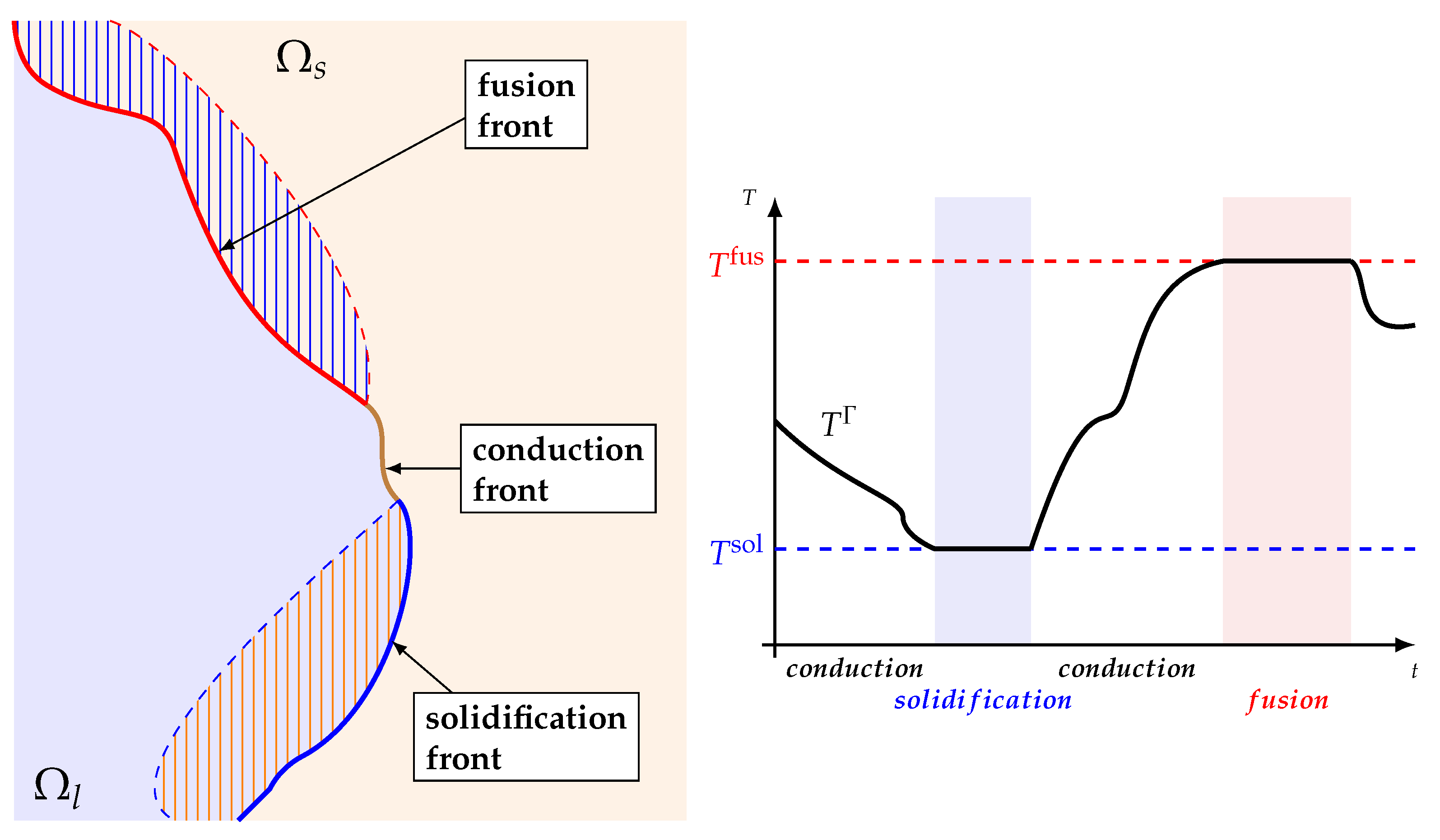
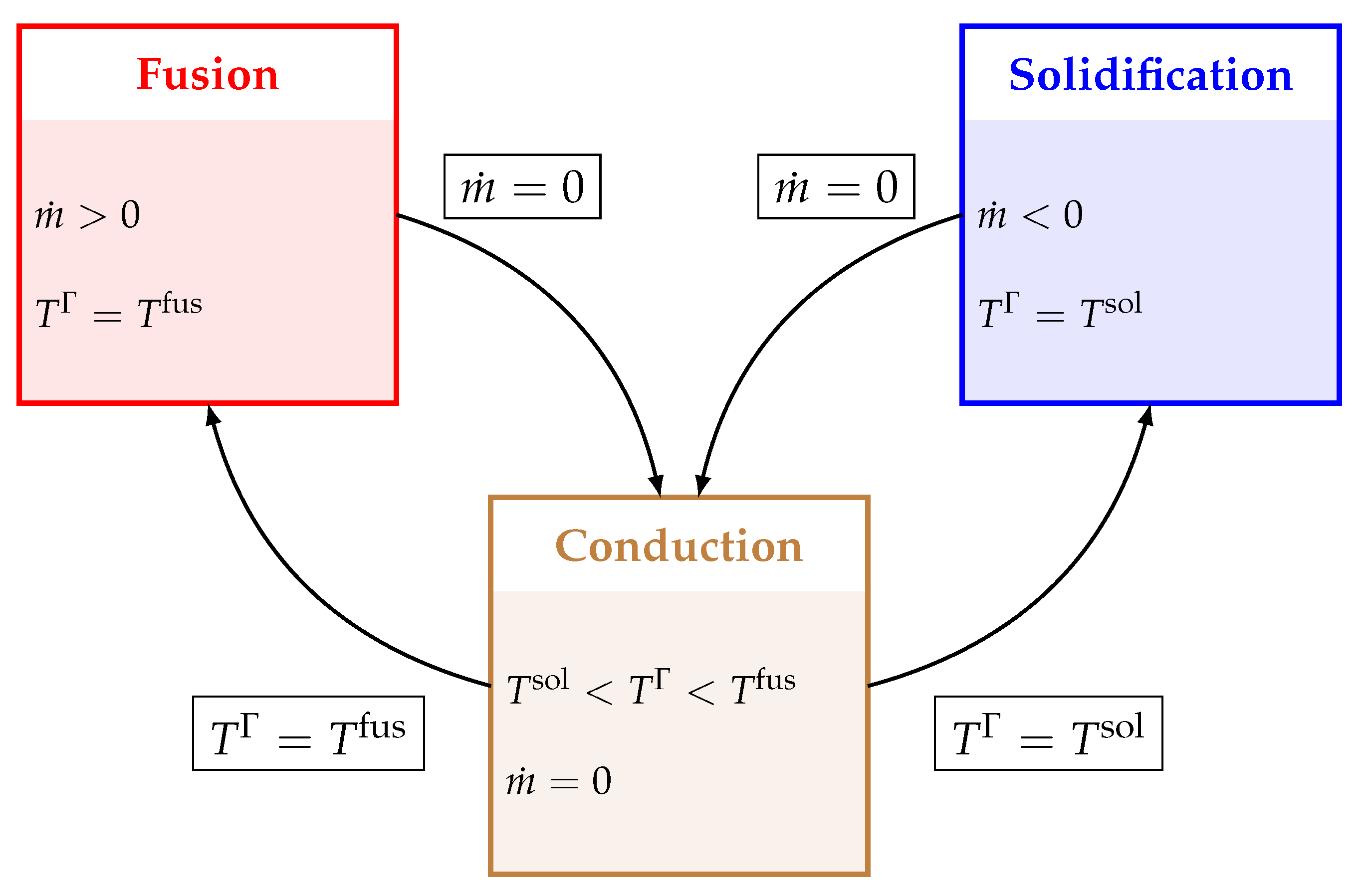
2.3. Conditions at the Phase Front

2.3.1. Stefan Condition at the Moving Phase Front

The interface Γ modeling the moving phase front, is represented by the color function χ , and, is located at δ Γ with normal n Γ and is moving at velocity v . The model describing its displacement is based on the conservation of mass and energy across it: the so-called Stefan condition [4,13,14]. Indeed the heat fluxes φ on each side of Γ and its magnitude in the normal direction are given by Fourier’s law as, k = l , s
φ k = λ k T k , φ k = φ k · n Γ ,
where λ , T are the conductivity and temperature in the vicinity of the front. The heat fluxes on both sides (liquid and solid) of the phase front are a priori different in terms of direction and magnitude, and their difference is directly linked to the phase change rate through the so-called Stefan condition:
m ˙ = φ l φ s H * ,
where m ˙ is the mass flux per unit area crossing the interface due to the phase change and H * is the strictly positive latent heat. H * takes either the value of the latent heat of fusion/solidification, H fus / H sol according to the sign of φ l φ s . If φ l φ s < 0 ( m ˙ is negative), the liquid is solidifying and H * = H sol . Otherwise the solid is melting and H * = H fus . Thus:
H * = H fus if φ l φ s > 0 , H sol otherwise .
Moreover written in terms of density and velocity, we can deduce the phase front velocity as a function of the mass flux m ˙ and the local density ρ as
v = m ˙ ρ n Γ .
The local density is determined according to the composition of the solid/liquid phase at the vicinity of the interface. Assuming an immobile solid ( u s = 0 ) leads to consider that the thermal flux jump between the phases which generate some motion has to be taken into account in the liquid.
The velocity of the interface is then deduced as being
v = u k m ˙ ρ k n Γ ,
where u k is the velocity of the phase k at the vicinity of the interface. Here, notice that the phase change imposes a velocity at the interface only if the densities of the phases are different, and, if the mass flux is non zero. Equation (14) is verified in both phases at the vicinity of the phase front, therefore the following condition is verified:
v = m ˙ ρ s n Γ = u l m ˙ ρ l n Γ u l = m ˙ 1 ρ l 1 ρ s n Γ .
Notice that, if the liquid and solid normal heat fluxes are equal, i.e., φ s = φ l , then the front remains static and we observe a pure heat conduction situation. Contrarily in a solidification/fusion situation then φ l φ s is strictly non-zero and the phase front moves.

2.3.2. Interface States

Let us assume that two extreme temperatures at the interface can be reached depending on the materials’ composition: T fus the temperature of fusion of the solid phase, and, T sol the temperature of solidification of the liquid phase such that T fus T sol . Defining the phase front temperature T T Γ for any x Γ ( t ) and all t > 0 , we consider three possible so-called ‘states’ leading to three conditions at the front:
Solidification state m ˙ 0 T Γ = T sol ,
Fusion state m ˙ 0 T Γ = T fus ,
Conduction state T sol < T Γ < T fus m ˙ = 0 .
Notice that the phase front is moving for the first two situations while it is static for the last one, see Figure 1 for an illustration.
From those considerations we set the following thermal closures:
T = T sol , if m ˙ 0 ,
φ s · n Γ = φ l · n Γ , if T sol < T Γ < T fus ,
T = T fus , if m ˙ > 0 .
Notice that the conduction equation φ s · n Γ = φ l · n Γ is a consequence of the relation m ˙ = 0 , see (11). In the conduction state, the temperature must be deduced from the conduction Equation (20). These conditions are recalled in the logical diagram on Figure 2.
As a final remark of this modeling section let us point out that in the case of homogeneous liquid and solid density, ρ l = ρ s then the right hand side of Equation (3) is identically null, and it amounts to solve a classical incompressible condition. Otherwise, when ρ l ρ s , the right hand side implies a volume change along with mass transfer between the phases. Finally system (3)–(6) along with BCs (8)–(9) is closed with phase front conditions (19)–(21). The numerical method designed to solve this problem is presented in the next section.

3. Numerical Methods

3.1. Rationale

The numerical method employed to solved the previous system of PDEs is inspired, partly re-used from Bois et al. [15,16] and implemented into the open-source code TrioCFD [12]. The code TrioCFD has been originally designed to deal with liquid/vapor applications. Contrarily, our context involves solid/liquid phase changes, and, therefore, the possible creation and presence of solids with the specificity that solid and liquid can be different pure materials. Consequently the original numerical methods in TrioCFD demand evolution and adaptation to fit with this solid/liquid phase change context. Namely, the one-fluid Navier–Stokes (NS) equations are solved by a prediction-correction scheme. For our context this demands to be penalized in the solids using for instance some Immersed-Boundary-Conditions (IBC) technique [9]. The phase change front evolution is captured by a front-tracking (FT) method [5] where the interfaces are tracked with a d 1 moving surface mesh, where d is the space dimension. This moving mesh technique is further coupled with a Volume-Of-Fluid (VoF) method employing a Level-Set (LS) distance function [17] in order to ensure a semi-local mass conservation. At last a Ghost Fluid Method [1] is used to solve the heat transfer within each phase separately. In this section we present the main aspects of the numerical methods developed in TrioCFD and their evolution to fit our context.

3.2. Time Discretization and Model Coupling

For the sake of clarity, an Euler explicit time discretization scheme is considered in this work. The time segment [ 0 , T ] is split into successive time-steps [ t n , t n + 1 ] with Δ t Δ t n = t n + 1 t n > 0 and n N . In what follows we identify any variable or parameter ϕ at time t n as ϕ n . Velocity and position of the materials are known at t n . Then the models describing the fluids, interface and solids are solved successively in a mildly coupled manner. Namely the velocity is first updated by the monolithic penalized NS equations. Secondly, the phase front is displaced due to the new temperature profile generating some phase changes so that the color function χ must be updated. Thirdly, the temperature field is computed within each phase by solving the heat equation over the time-step. Note that the extension to high order of accuracy in time via Runge-Kutta schemes, recast as successive explicit Euler steps, is feasible within TrioCFD but out of the scope of this work.

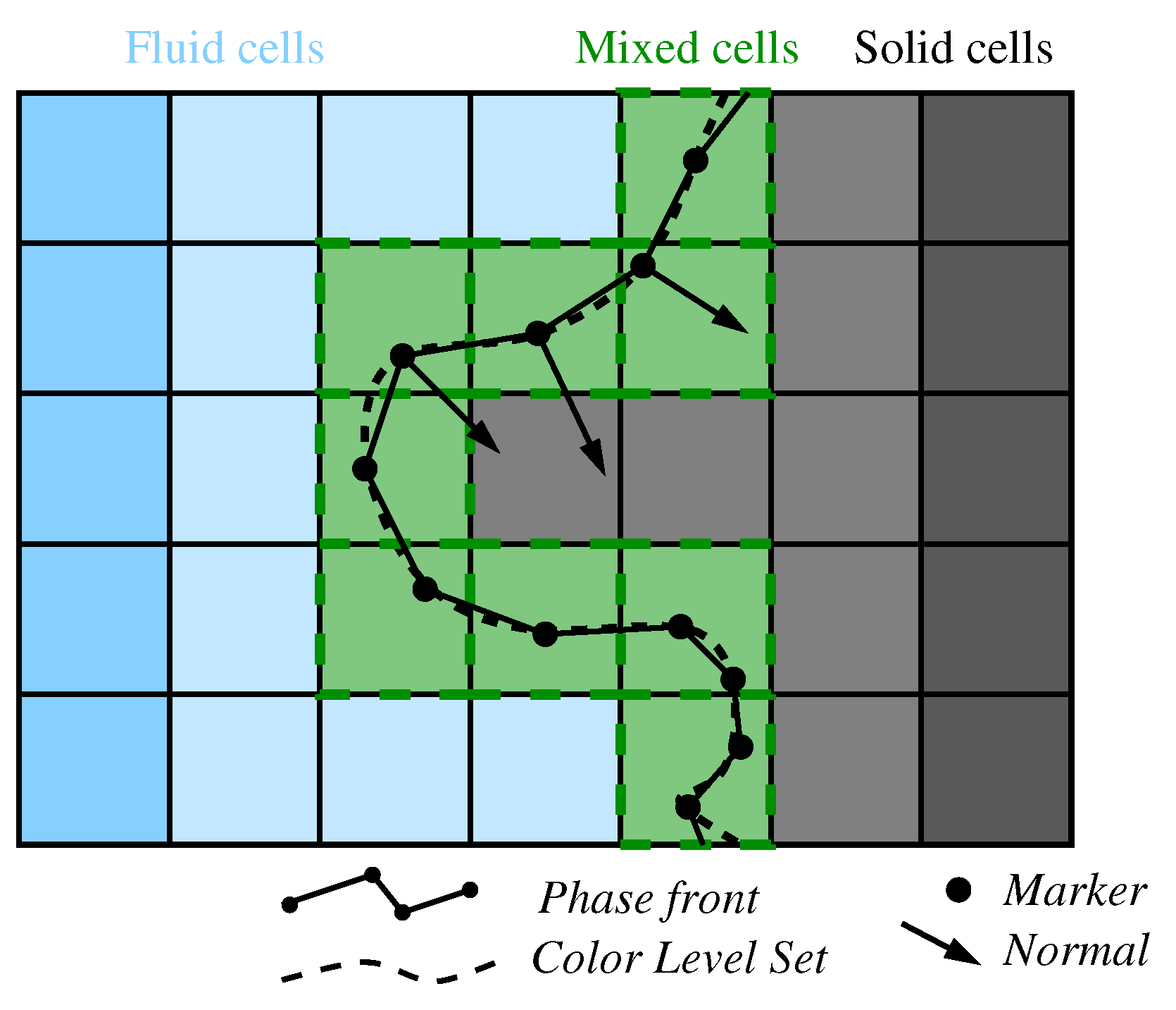
3.3. Mesh and Front Representation

Computational Mesh

The computational domain at time t n is an evolving polygon/polyhedron Ω ( t n ) in 2D/3D. For the sake of clarity we present the 2D discretization reminding that the 3D extension follows the same concepts. Ω ( t n ) is covered without gap nor hole by an unstructured mesh made of fixed quadrangles, also called cells, and denoted by ω c for c = 1 , , N c . This mesh is referred to as M Ω .
The phase front of dimension d = 1 , represented by the color function χ , is meshed by a list of ordered points, called markers, each referred to by ξ k , k = 1 , , N k . This 1D mesh is called M χ and evolves within M Ω . The number of markers N k may increase or decrease to ensure an acceptable geometrical quality of the phase front. At each marker we compute the normal as the sum of the two normal vectors of the front segments impinging at the marker.
As such any quadrangular cell can be either ‘pure’ or ‘mixed’ if M χ crosses ω c or not. If ‘pure’, the cell is entirely included in the liquid phase or in the solid one. If ‘mixed’ then at least one or two pieces interface segments cross the cell splitting it into pure liquid and solid states, see Figure 3.

3.4. Navier–Stokes Discretization via a Penalized Prediction-Correction Method

The Navier–Stokes equations are solved using a so-called prediction-projection method on a staggered grid with a Marker-And-Cell (MAC) discretization [3]. The velocity components are located at the cell faces, while the scalar transport variables (pressure, temperature, level set function) and the thermodynamic properties (density, viscosity, thermal conductivity, heat capacity) are computed at the cell center. This method computes the velocity field on the whole domain, and so, a penalized method is used in combination to ensure a vanishing velocity in the solid. For this purpose, the penalized method introduced initially in Belliard [11] without phase change has been adapted to our context.
The time-dependent incompressible Navier–Stokes equations are solved explicitly in time using the standard projection method [2]: from the quantity known at t n , the pressure P n + 1 and velocity u n + 1 are deduced using the prediction-correction method [16], leading to the discrete momentum equation. The spatial discrete operators considered in this study correspond to those initially implemented in TrioCFD [18] and are identified with index h. In particular the convection operator refers to the QUICK scheme (Quadratic Upstream Interpolation for Convective Kinematics [19]) while the diffusion operator corresponds to a usual second order finite difference scheme. Let us describe these two prediction and correction steps in the following.
Penalized prediction: This step consists in using an Euler explicit time scheme to compute a predicted velocity u * neglecting the pressure term in (4). The zero-velocity constraint on the solid phase is dealt with by adding a penalization term which is controlled by an arbitrarily small parameter η = 10 12 1 .
Introducing the notation:
T = h · ( u n u n ) + 1 ρ n · ( μ n ( h u n + h T u n ) ) + g ρ l ρ n β ( T n T 0 ) ( 1 χ n ) g ,
the predicted velocity, u * , is computed as:
u * = u n + Δ t T χ η u * .
Reformulating (23) as
u * = 1 1 + χ η u n + Δ t T ,
we notice that, numerically, the predicted velocity u * vanishes in the solid phase, where χ equals 1, as ( 1 + χ η ) η 0 , while it remains unchanged in the liquid phase where χ = 0 .
Penalized correction: Following [11], the penalized correction consists in computing the corrected velocity which fulfills the constraint (3) as
u n + 1 = u * + Δ t ρ f n h P n + 1 + χ η ( u * u n + 1 ) ,
where P n + 1 has to be preliminary determined and ρ f n corresponds to an averaged density at the current face usually equal to ρ l in the liquid phase. The correction step presented in [11] does not take into account any phase which violates the non-zero divergence Equation (3). On the other hand, the numerical discretization of this term introduced initially in TrioCFD [15] uses a signed distance (defined in Section 3.5), and, has been derived without considering any penalized method in the context of water vapor/liquid applications, considering therefore a ratio of density of about 1000 between both phases. Our context, and others in engineering, witness density ratio of order unity and the presence of solid or quasi-solids.
Therefore, we propose here to integrate in any mixed cell the term, m ˙ 1 ρ l 1 ρ s appearing in (3), along the interface to get a discrete volume term as:
ζ n ζ ( t n ) = Γ n ω c ω c m ˙ n 1 ρ l 1 ρ s .
Here Γ n ω c ω c is the length (or surface in 3D) of the front in the given mixed cell, and, m ˙ n corresponds to the mass flux across this front (detailed later in Section 3.5).
Next, the classical correction step [15] is reformulated regarding the contribution of the penalized term introduced in (23). The pressure term P n + 1 is then deduced from
η η + χ h · 1 ρ f n h P n + 1 = 1 Δ t h · u * + 1 Δ t ζ n .
However, the term ζ n is a priori defined in a mixed cell. Hence the parameter η , intended to go to zero in cells where the solid is present, generates that the numerical contribution of the phase change ζ n in (27) is numerically canceled. To overcome this undesirable behavior, we made the choice to affect this discrete volume change term to the closest pure liquid cells. Recall that these liquid cells are not subject to any penalization term. This choice is somewhat justified by the fact that only the liquid has to endure the whole volume change constraint, while the solid has to maintain a zero-velocity. This numerical algorithm allowing to transfer the mixed cell contribution of ζ n to the closest pure liquid cells is not detailed here but relies on crude interpolation techniques. As such the contribution of ζ n for a given mixed cell is consistent with the corresponding global volume change computed in the corresponding pure liquid cells.

3.5. Interface Treatment: Motion and Geometrical Regularization

As already mentioned the phase front is represented by a sharp interface, that is a surface mesh made of straight segments in 2D (and co-planar triangles in 3D).

3.5.1. Displacement

The displacement of the markers drives the motion of the interface. A level-set method is adopted for capturing the phase front interface dynamics. Γ is represented using the zero level of a continuous surface Level Set (LS) function ϕ .
Γ ( t ) = x Ω , s . t . ϕ ( x , t ) = 0 ,
where the level set function is represented by a signed distance function ϕ ( x , t ) = ± | d | , where d represents the shortest distance from any grid point to the interface with the signs ϕ > 0 in the liquid phase and ϕ < 0 in the solid one. The advection of the level set function is performed by the non-conservative equation
ϕ t + v · ϕ = 0 ,
where v is physically valid only at the interface Γ but is needed in the small region close to it. To ensure that the signed distance function property of ϕ is preserved during the computations, ϕ can be periodically re-initialized, loosing as such the conservation of the phases. To counter-fight this effect, a Volume-of-Fluid (VoF) method is supplemented to compute the conservative evolution of the colour function χ . The discrepancy between the conservative VoF volumes and the LS ones is used in the regularization/smoothing algorithms.

3.5.2. Regularization/Smoothing

In order to preserve sufficient geometrical quality of the interface mesh during the simulation, regularization and smoothing algorithms are employed within TrioCFD. These geometrical modifications are performed under the constraint that the mass of each phase is conserved as best as possible. First, the remeshing procedure maintains the mesh edge length within a prescribed range. It relies on deleting markers on small edges, or adding some at the middle of too long ones. As such the connectivity of the interface mesh does change. Second, the smoothing procedure consists in a regular redistribution the markers without connectivity changes along/on the interface mesh in 2D/3D. Somewhat it corresponds to a Laplacian smoothing on the marker position under the constraint that the associated changes of volume/mass remain controlled. The detailed description of these algorithms can be found in [15,16].

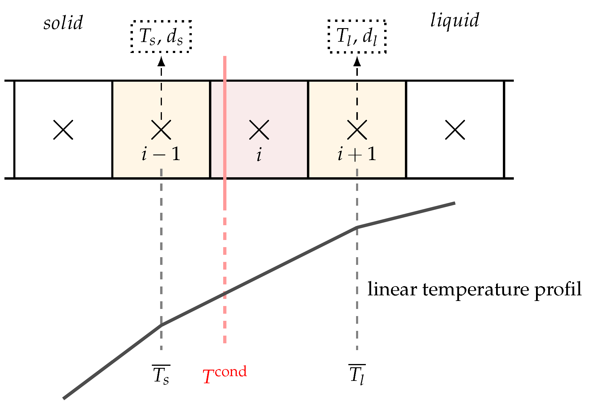
3.6. Ghost-Fluid Approach for Heat Transfer Equation

The ghost-fluid approach is employed to solve the energy equation in each phase governed by (5) in terms of temperature variations. The moving phase front renders this resolution difficult because the velocity and heat flux are discontinuous across it. To leverage this difficulty the Ghost-Fluid approach is employed as it replaces the discontinuity by a continuous extension of Eulerian fields across the interface. The temperature being defined at the cell-centers, so will be the temperature gradient normal to the interface T · n and the phase-change rate m ˙ .

3.6.1. Temperature Gradient and Rate of Change

In the vicinity of the interface, first, based on linear extrapolation of the liquid temperature from pure liquid cells, the ‘liquid ghost temperatures’ are extrapolated in the ghost cells. From the interface temperature, T Γ , assumed to be given (see later for its determination) and the distance function, d, the normal component of the temperature gradient at the interface, T · n , is readily obtained for both phases as
( g T s · n ) = T Γ T s d , ( g T l · n ) = T Γ T l d .
As such these cell-centered fields represent the normal heat fluxes at the interface and can be computed for any liquid or solid cell. Once mixed and pure solid cells get a gradient, it is possible to assign a ‘liquid ghost temperature’ in the solid phase and, vice-versa, a ‘solid ghost temperature’ in the liquid phase which are further used for the next time-step.
Using the ghost gradients in each phase, we are able to calculate m ˙ corresponding to a discrete mass rate of change due to phase changes in mixed cells:
m ˙ = λ l ( g T l · n ) λ s ( g T s · n ) H * ,
where H * is the enthalpy of fusion or solidification which depends on the interface state (see next paragraph). m ˙ in (31) is a priori only defined in mixed cells, but a prolongation is carried on to extend this phase change rate m ˙ in the vicinity of the interface, that is in pure solid cells.

3.6.2. Interface Temperature/Interface State

In our model, and as shown in Figure 1, the interface temperature can only vary between T fus and T sol . As such the ‘interface state’ becomes a variable of interest and we follow it with an Eulerian cell-centered field which takes values S / C / F for solidification/conduction/fusion cases. At each time step, the state of the interface is updated in mixed cells and in their vicinity, following the logigram Figure 2. The interface temperature in mixed cell is deduced using the following relation
T Γ = T fus if the mixed cell is in fusion , T cond if the mixed cell is in conduction , T sol if the mixed cell is in solidification .
where T cond is the last unknown when conduction occurs. To determine T cond in this work we rely on the heat flux equality through the interface. A simple linear interpolation is performed between two local averaged temperatures/distances of the solid and liquid phase, T s ¯ , T l ¯ , d s ¯ , and d l ¯ . While in 1D the situation is simple and there is no need to compute any of those averaged values, see Figure 4, in 2D and 3D there is no unique temperature and distance to the interface to rely on. In practice one computes the average of pure cell values considering the 3 × 3 stencil around the current cell. At last the interface temperature is obtained thanks to the formula
T cond = λ s T s ¯ d l ¯ λ l T l ¯ d s ¯ λ s d l ¯ λ l d s ¯ .
This equation ends the description of the numerical method which has been partly reemployed and adapted within the simulation code TrioCFD. In the next section a validation and verification campaign is carried on.

4. Validation and Verification Test Suite

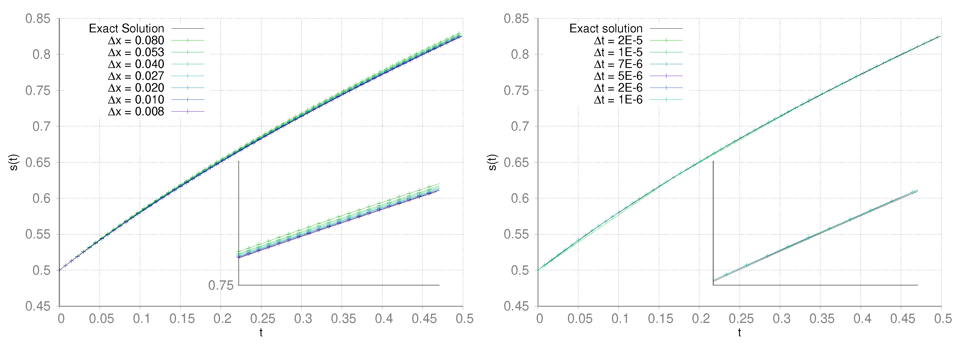
4.1. Stefan Problems

In order to validate our numerical approach we simulate the so-called 1D Stefan problem. This test case has an analytical solution [4,13] towards which we can observe the convergence of the space-time evolving numerical solution as the mesh/time steps are refined. The problem consists in simulating the 1D solidification (resp. fusion) of an homogeneous material, for which the solid and liquid phases have the same material properties. The semi infinite computational domain corresponds to Ω = Ω s ( t ) Ω l ( t ) with the solid represented by Ω s = [ 0 , s ( t ) ] where s ( t ) is the location of the moving front in-between for any time t > 0 . A semi infinite liquid domain should stand on the right of Ω s at constant solidification temperature T sol but we restrict it to Ω l = [ s ( t ) , 10 ] so that the right boundary is too far to interfere with the computation. An external temperature T ext < T sol is enforced at the left boundary of Ω s . The aim is to compute the position of the interface s ( t ) and the temperature profile T ( x , t ) . The governing equations of the 1D Stefan problem are:
T t ( x , t ) = α 2 T x 2 ( x , t ) , β d s d t s ( t ) , t = T s ( t ) , t ,
where α = λ ρ C p , β = ρ Δ H sol λ , and for all x Ω and t [ 0 , t final ] . The boundary and initial condition are given by: T ( 0 , t ) = T ext , T ( s ( t ) , t ) = T sol , and s ( t = 0 ) = 0 . The unique solution of this problem is given by [4]:
T ( x , t ) = T ext + ( T sol T ext ) erf x 2 α t erf ( k ) ,
s ( t ) = 2 k α t , k e k 2 erf ( k ) = 1 β α π T sol T ext ,
where erf is the error function. k is approximated by Newton’s method on the last equation and further substituted into (35) and (36)-left. We consider a rectangular domain Ω s of 4 units in length by 0.5 in height. This domain is paved by N x cells in length and N y = 9 cells in height, N x is subject to take increasing values.
Since our modeling does not handle the creation of solid initially, our simulations start with a pre-existing solid. Hence we assume an initial front position at s ( t init ) = 0.5 and the parameter values α = 1.0 , β = 1.0 and T ext = 1.0 . The initial temperature of the solid is given by the exact solution: T s ( x , t init ) = 1 + 1 erf ( k ) erf ( x 2 t init ) where t init = 0.2893 . The initial temperature and velocity of the fluid are set to 0. Then we set the following constant values for the physical parameters: λ = 1 , C p = 1 , μ = 1 and H fus = H sol = 1 . Moreover we consider two different densities for the liquid and solid: ρ l = 2 and ρ s = 1 . Then two configurations are simulated: one where T fus = T sol , then one for which T fus T sol .

4.1.1. Configuration T fus = T sol = 0

The results in Table 1 gather the errors in norm L 1 , L 2 and L obtained by our numerical modeling for decreasing values of Δ x . Each simulation is performed until the final time t max = 0.5 with a fixed time step equal to Δ t = 10 4 . The results in Table 1 show a reduction of the errors, proving numerically that the numerical method converges at order 1 as expected.
Next, Figure 5-left shows the position of the interface over time for each mesh compared to the exact position. Each simulation correctly approximates the exact solution, and, the finer the mesh the better the approximation (see the zoom). Figure 5-right shows the position of the interface over time for different time steps with a fixed space step Δ x = 0.01 corresponding to N x = 400 . We observe that our numerical results fit relatively well the exact solution. If we further increase the time step, the method diverges because the coupling of the equations requires a small time step for the numerical method to remain stable. This restricted time step leads to a situation for which the error produced by the discretization in time is much smaller than the spacial error.

4.1.2. Configuration T fus T sol

Here, the solidification temperature is set to T sol = 0.5 and the melting temperature to T fus = 0.5 . In this situation, while the liquid is heated up on the right boundary, it cools down at the interface s ( t ) . Hence, one expects a scenario for which a cooling period at the beginning of the test case, corresponding to a pure conduction period, is followed by a solidification period. No analytical solution is available. It is possible to assess the starting time of the solidification which corresponds to the time when the temperature at the interface reaches T sol by t = 0.2748 . In Figure 6 we plot the interface position s ( t ) as a function of time. We clearly observe no motion of the interface (conduction state) at the beginning, then the displacement of the interface and its progressive stop (solidification state), and no motion anymore (back to conduction state). We can observe that the time of transition to solidification is well approximated by t 0.27 . The solidification stops around t 0.8 , but there is no analytical solution to compare this result with. Stefan problem was a sanity check used to prove that the model solved by our adapted numerical method in TrioCFD is able to capture the phenomenology generated by a moving interface driven by solidification/fusion and conduction periods. More sanity checks have been conducted but we omit them in this paper.

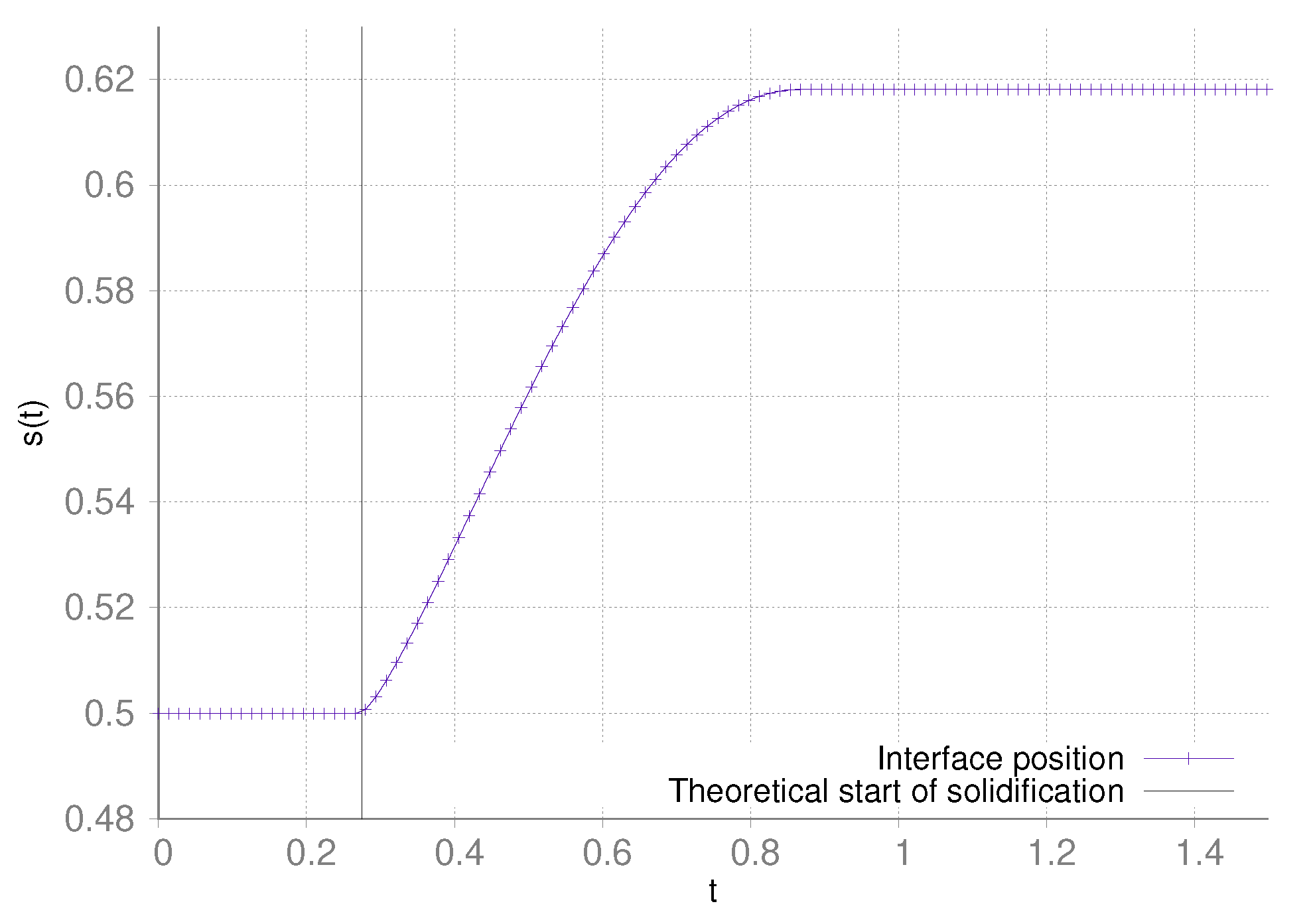
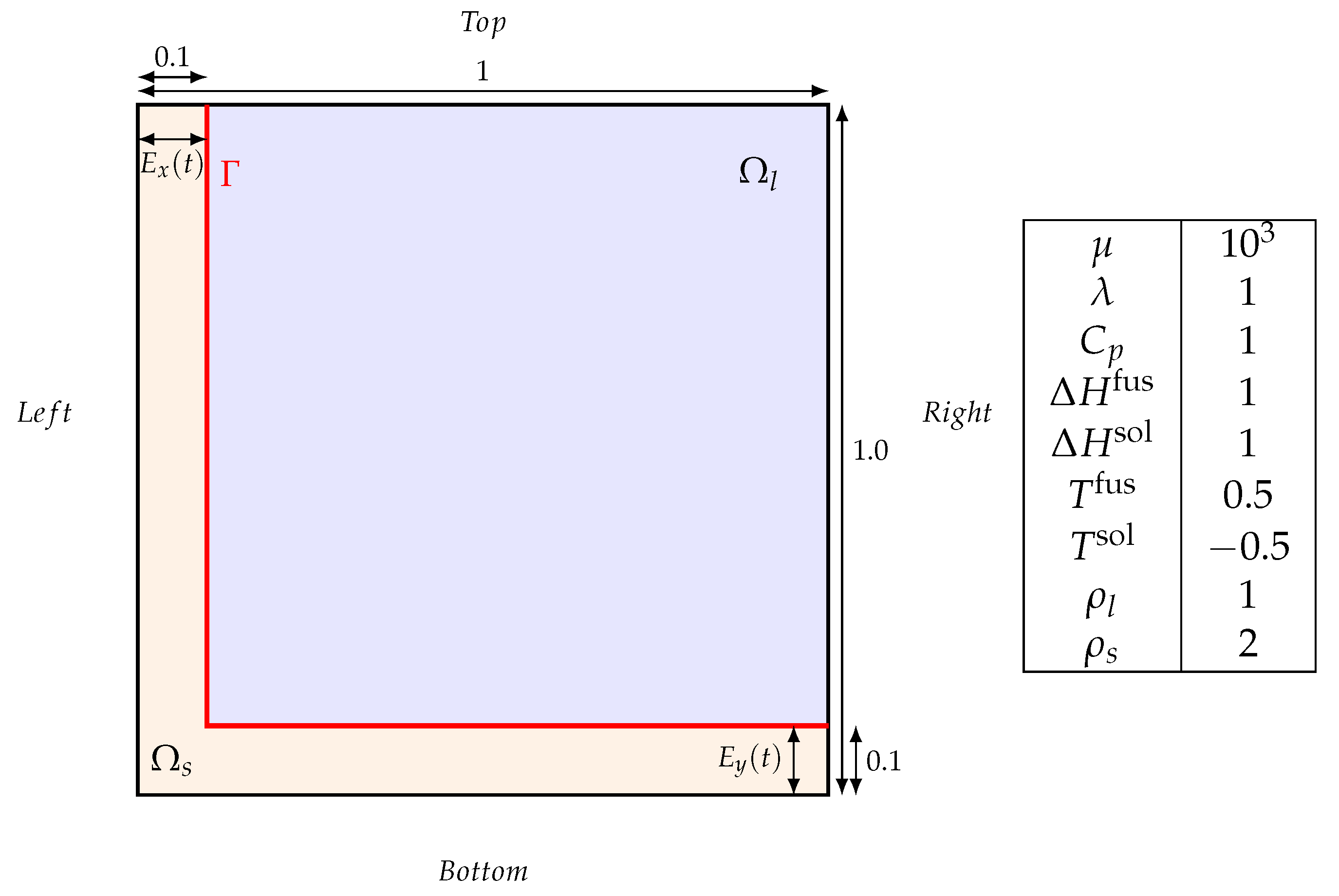
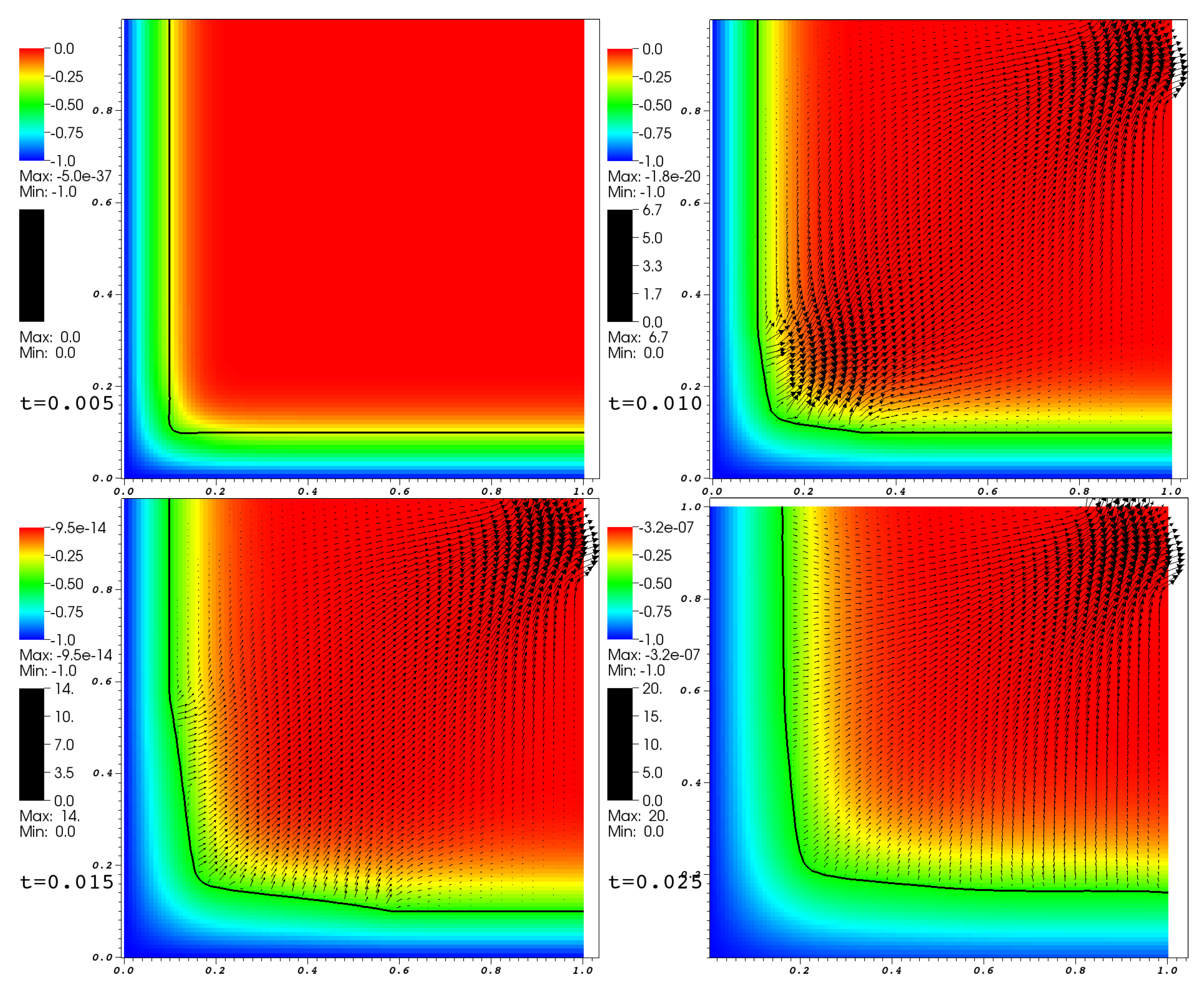
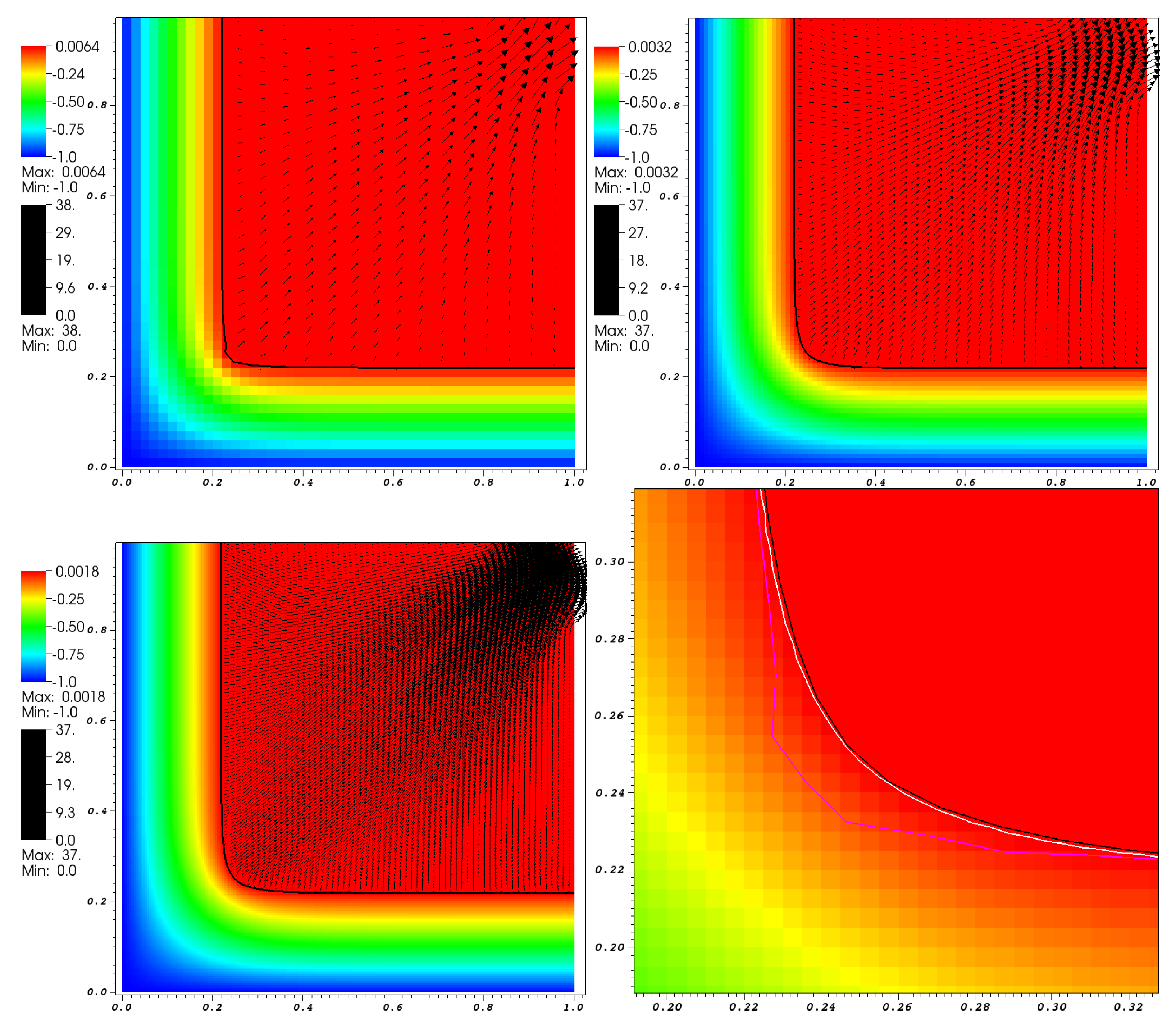
4.2. Two-Dimensional Corner Stefan-like Test Case

This double Stefan-like test case consists in the solidification of a semi-infinite 2D domain with a corner, see a analysis and numerical studies in [20,21,22]. The fixed computational domain is Ω = [ 0 ; 1 ] 2 which initially is split into a liquid phase at rest Ω l = [ E x ( t = 0 ) ; 1 ] × [ E y ( t = 0 ) ; 1 ] at solidification temperature T sol and a solid one Ω s = Ω Ω l . The initial corner shaped solid thickness is set to E x ( t = 0 ) = E y ( t = 0 ) = 0.1 . The mesh is set to 110 × 110 cells and the time step is fixed at Δ t = 10 4 . Initial temperature is constant at T = 0 . The temperature at boundaries x = 0 (bottom) and y = 0 (left) is fixed at a temperature T ext = 1 lower than the solidification temperature, T sol = 0.5 , so that the solidification phenomenon starts because of these cold boundaries. Notice that in this test T sol T fus . The liquid domain is closed but for the top-right corner where an opened BC is set for the liquid to escape if appropriate, the rest of the boundaries are of slip-wall type. This initial configuration is represented in Figure 7-left along with its associated physical parameters. Far away from the corner, the computed solution should be close to the classical 1D Stefan solution in x and y directions. Contrarily, in the vicinity of the corner, genuine 2D effects are expected.
Figure 8 shows the results obtained for four successive times t = 0.005 , 0.01 , 0.015 , and 0.25 . At time t = 0.005 (top-left), the interface has not yet reached the solidification temperature, and, consequently, the interface state is in pure conduction, there is no phase change, nor any movement of the front. On the other hand, we observe a cooling phenomenon occurring from the boundaries. More importantly a non-constant temperature profile is observed on the liquid side proving that heat conduction takes place across the interface. At time t = 0.01 (top-right) in the vicinity of the interface, close to the corner, solidification starts, while, far from the corner, the pure conduction situation still occurs. We observe that this part of the interface close to the corner is set in motion, moves, deforms, and retroactively generates a velocity on the liquid because of the change of volume linked to the difference of densities. Also one observes that the liquid tends to escape from the top-right open boundary as expected. On the figure at time t = 0.015 (bottom-left) the solidification state propagates along the phase change front symmetrically upward and rightward. Finally on the panel at time t = 0.025 (bottom-right) the solidification state has reached the whole length of the front, since the latter is at a temperature T sol = 0.5 . As such the whole solidification front is set in motion.
Thus, this test case allows to simulate different features of the implemented numerical method: pure conduction through the front, solidification of the liquid setting in motion of the front and changing the temperature and velocity fields, and the regular transition between the states. Moreover, the coupling with the penalization method allows to maintain and ensure a zero-velocity in the solid. At last we have verified that far away from the corner the exact 1D Stefan solution is retrieved until the effects of the 2D corner interfere.
At last, a mesh independency study is presented in Figure 9 by comparing results for a similar test case (only modified by using T sol = T fus = 0 and thus leading to less CPU-time consuming) on three successively Cartesian refined meshes: a coarse ( 50 × 50 cells), intermediate ( 100 × 100 cells) and a finer mesh ( 150 × 150 cells). As expected the refined meshes capture more accurately the flow, the fileds and the interface location. The numerical results seem to converge appropriately as can be seen on the fourth panel where the location of the interface is plotted in purple/black/white lines for the coarse/intermediate/fine mesh respectively. Some numerical comparisons against other methods can be also found in [21,22] for instance.

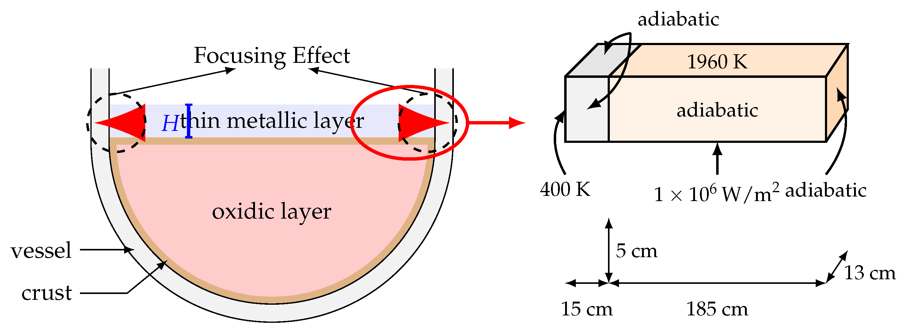
4.3. Focusing Effect within a Thin Metallic Layer

In this last test case, we propose to use our numerical modeling approach in a more industrial-like application. In the context of nuclear severe accident, one important research interest is the simulation of a thin metallic liquid layer on the top of a corium pool. This configuration occurs when an In-Vessel Retention (IVR) strategy is considered which consists in sustaining the integrity of the reactor pressure vessel by External Reactor Vessel Cooling [23,24,25,26,27]. To estimate the success of IVR strategy, an accurate evaluation of the heat fluxes that the corium pool imposes to the vessel lower head is needed. Due to the ablation of the vessel wall and to thermo-chemical effects, a thin metallic layer, in direct contact with the vessel wall, may lay on top of the corium pool. Such a thin layer may drastically increase the heat flux on the vessel up to possible failure of its integrity [28]: this is the so-called heat flux ‘focusing effect’. In the present work, simulation of the interaction between the thin metal layer and the vessel wall are considered in order to evaluate the effects of the phase change phenomena compared to the work done in [29]. Indeed, in [29] the vessel was not simulated and only single-phase thermalhydraulics simulations were performed (with a temperature set equal to the steel fusion temperature at the boundary). Thus, the objective of this current test case is to genuinely simulate the vessel in order to observe the impact of the melting phenomenon. Two-dimensional and three-dimensional simulations are proposed.

4.3.1. Test Case Description

A sketch of the configuration is presented in Figure 10. The global IVR context is illustrated on the left side. The actual geometry considered in the present simulations is depicted on the right of the figure. This geometry focuses on the coupling between the thin metallic layer and the vessel. The fixed global length (x-axis) is set at L = 200 cm, initially 15 cm for the solid vessel and 185 cm for the liquid metal layer. A fixed height (z-axis) of H = 5 cm is assumed while the width is in the range [ 0 , 13 cm]. Regarding thermal boundary conditions, the bottom surface of the liquid ( z = 0 ) is subjected to a constant heat flux of 10 6 W/m 2 . The front, back (perpendicular to the y axis) and one lateral (at x = 2 m) walls are adiabatic as well as for the solid bottom boundary. Contrarily the left lateral wall is set at a fixed temperature 400 K representative of the external vessel wall cooling by water nucleate boiling. At the top surface, fixed temperature is imposed at 1960 K for the liquid and adiabatic condition is assumed for the solid. For mechanical boundary conditions, no slip conditions are assumed. The properties of steel are assumed to be constant as in [29] and gathered in Table 2. Note that this rectangular box setup differs from the actual axisymmetric vessel geometry but was considered in [29] because it corresponds to the geometry of the BALI-Metal experiment [30] used for validation purpose.

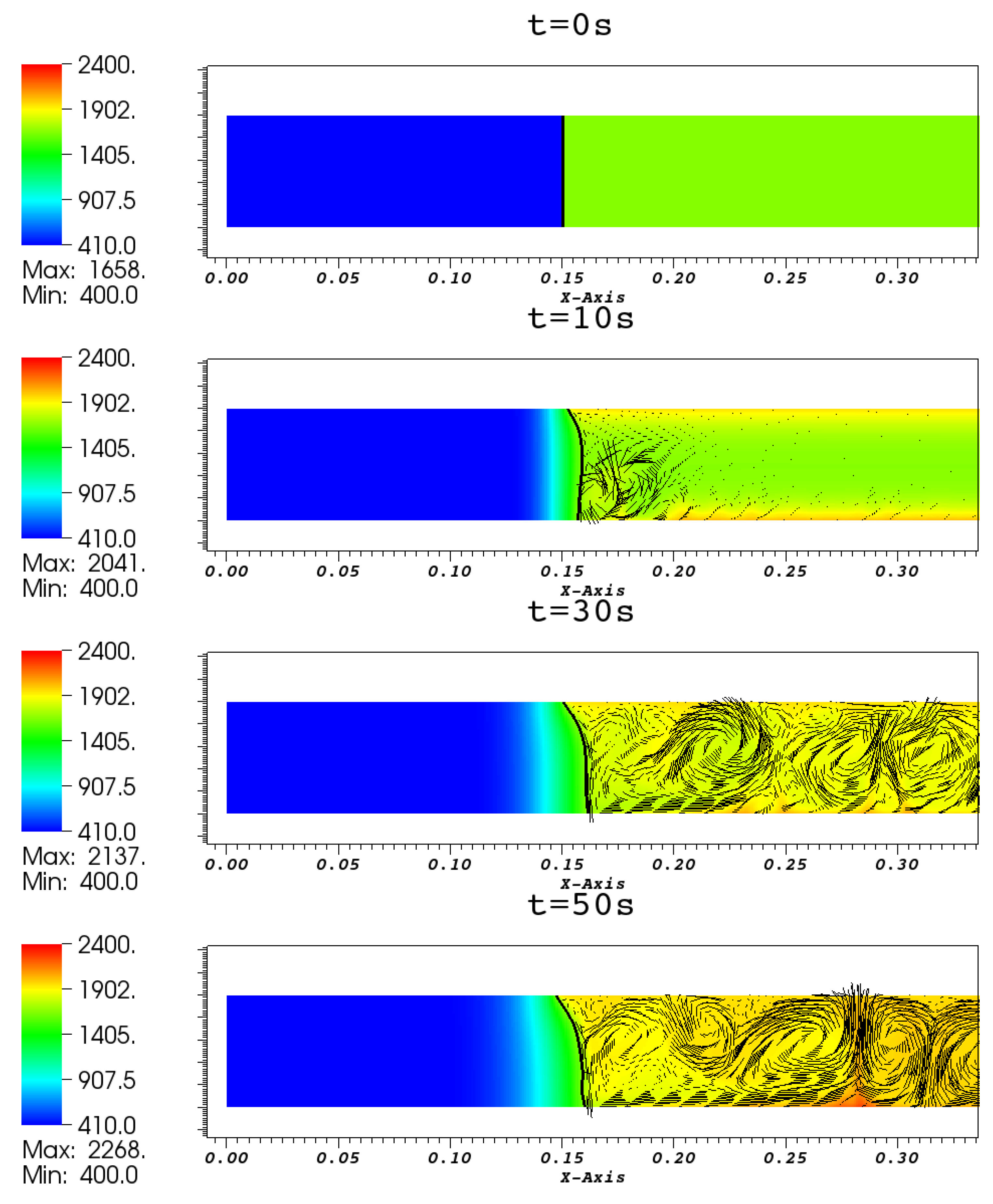
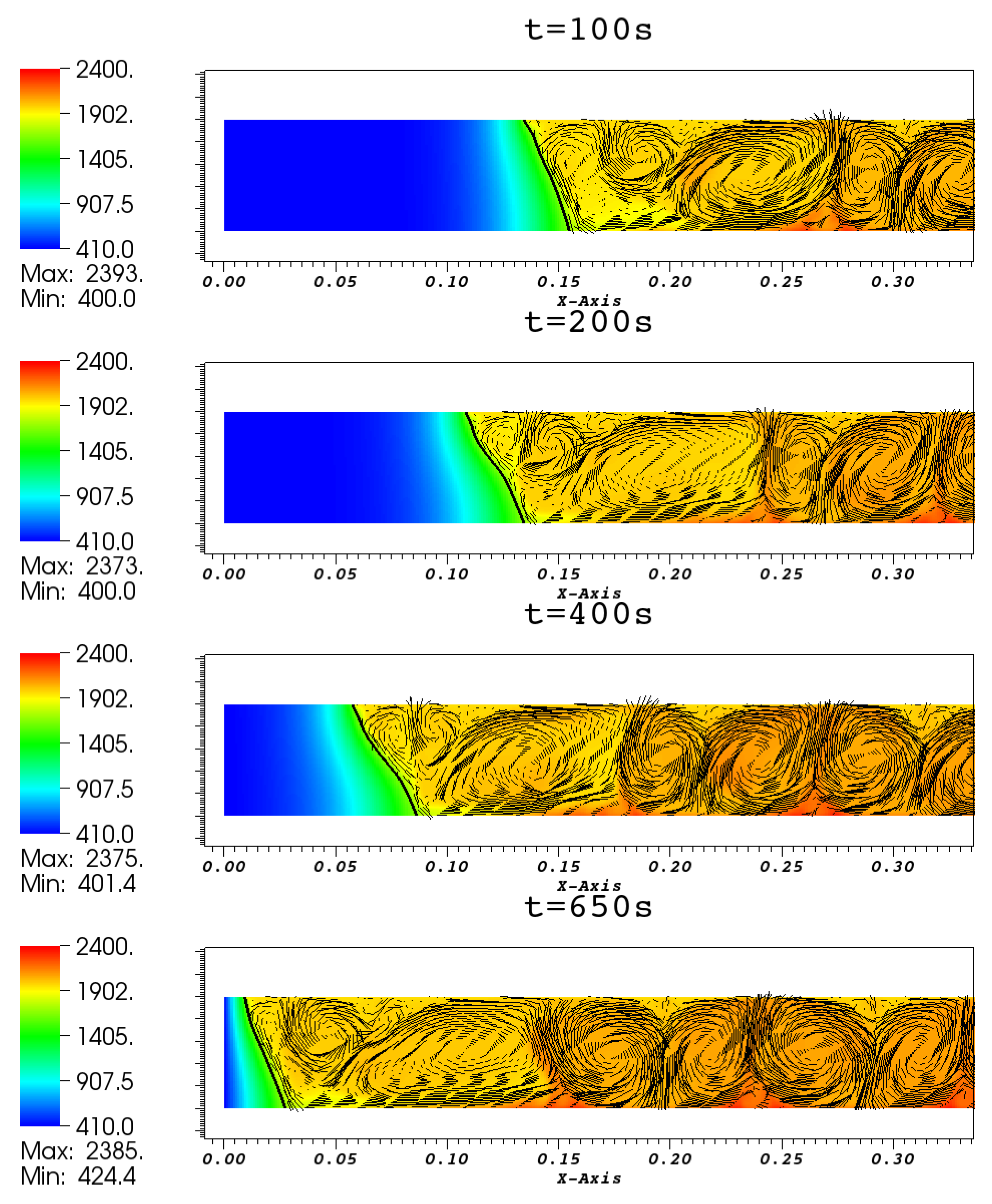
4.3.2. Two-Dimensional Simulations

First of all, results of 2D simulations ( z x plane) are presented in Figure 11 and Figure 12 in terms of the temperature and velocity fields computed in the thin metal layer and the vessel at different intermediate times and using a computational mesh constituted of 1200 × 100 cells. We observe the displacement of the interface in the transient regime and the establishment of a multi-dimensional flow related to thermal gradients in the liquid. It is interesting to note that at the beginning of the transient, because of the way the temperature field is initialized, the interface starts moving to the right: the liquid slightly solidifies (see Figure 11). It is only for t > 50 s that the vessel fusion occurs (see Figure 12). Near the interface, the vertical thermal gradients are more pronounced, reflecting the cooling effects near the interface. They are associated with a re-circulation that can be observed at different times in the figure. We also observe the setting up of Rayleigh-Bénard type convection cells far from the interface (and not influenced by the physical phenomena at the interface). This structure of the flow corresponds to the one expected and observed in the BALI experiment [30] and the simulations without taking into account the vessel presented in [26,29].

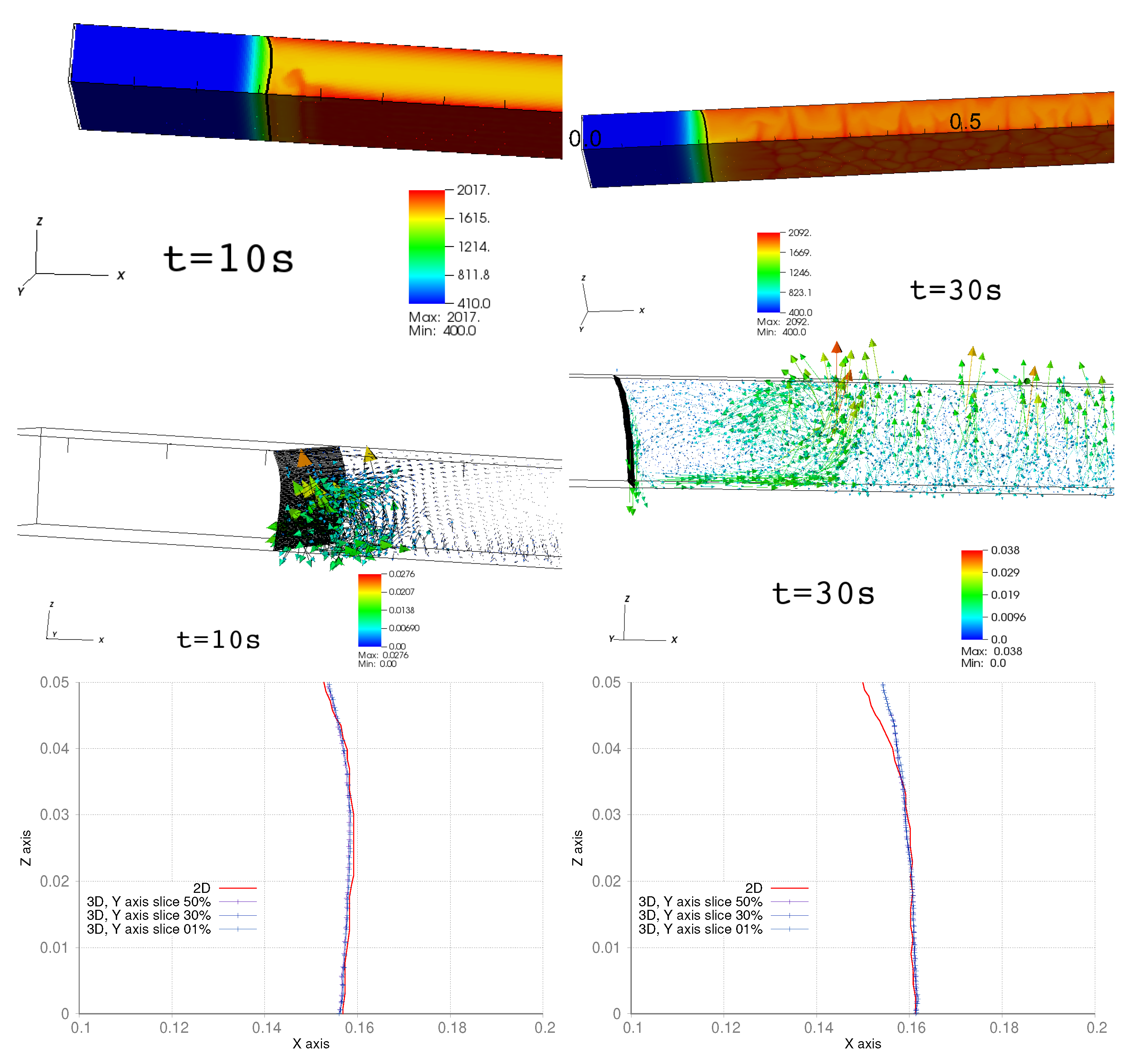
4.3.3. Three-Dimensional Simulations

Then, we present in Figure 13 results obtained for the 3D case with the same 2D input parameters given in Table 2 and Figure 10. At the top panel, the temperature field is presented while the velocity vectors and fusion front are given in the middle panel. The position of the interface for different slices orthogonal to the y axis is also depicted and compared to the interface computed in the previous 2D test case. According to the adiabatic boundary conditions applied on the front and back boundaries (perpendicular to the y axis), the main differences compared to the 2D case appear during the transient regime. Therefore the numerical results are presented at the very beginning of the simulation for two different times: 10 s and 30 s. As expected, the difference between 2D and 3D calculations remains limited in terms of the interface position because of these adiabatic boundary conditions on the front and back boundaries. Furthermore, these numerical results are intended to prove the ability of the code to handle the 3D displacements of the interface with phase change in the context of a complex flow. This proof of concept now demands more advanced and quantitative analyses. In terms of computation cost, this 3D simulation uses a computational mesh constituted of 1200 × 50 × 50 cells and has required ten days of computing time using 64 CPU cores. The parallelization of our numerical development relies on the MPI parallel version of TrioCFD.

5. Conclusions and Perspectives

In this paper, we focus on the modeling and numerical simulation of two-phase flow involving solid-liquid phase changes. In our context, the fusion and solidification temperatures may be different which implies that a transition zone may exist in between the phase changes. This situation may be encountered when considering corium as a pure (liquid or solid) material for the study of severe accidents in nuclear power plants for instance. The modeling, numerical methods, and simulation code, must be adapted. In this work, we have developed, adapted and extended from [11,16] a model and code based
  • on a monolithic Navier–Stokes system of equations penalized in the solid phases and adapted to the specificity of such phase changes,
  • on a Front-Tracking approach to follow the phase change front supplemented with a Volume-of-Fluid method to counter-fight possible lack of mass conservation,
  • on monolithic heat equation supplemented with the Ghost-Fluid approach to deal with the discontinuity at the front.
The numerical methods used to solve such a model have been presented in this paper. This numerical model has been further implemented/adapted in the code TrioCFD [12,18].
A numerical validation and verification campaign has been carried out, and, some results have been gathered such as the Stefan 1D and 2D validation tests and a more industrial-type 2D/3D test case corresponding to the analysis of the so-called ‘focusing effect’ pertaining to corium behavior in the realm of nuclear reactor safety.
The simulation tool, as such produced for general applications coupling liquid/solid with phase change, seems to be adequate to be used at a more operational level and this is one of our goal in a near future. From the numerical method point of view we plan to analyze the time-step determination, possibly considering implicit schemes. So far we have only used a semi-explicit time scheme with an ad-hoc time-step restriction. Moreover, a more in-depth study should be carried on to evaluate the accuracy of the thermal fluxes through the interface related to the use of the Ghost-Fluid method. This work takes a step forward in our general ongoing R&D effort to provide models and numerical methods for simulating the thermal-hydraulic behavior of a corium pool composed of different chemically reactive liquid phases with, possibly, liquid/solid phase change at their boundaries. The presented CFD results and, more importantly, the future ones will be used for engineering applications following an up-scaling methodology (see [31] for instance) in order to enhance modeling in the industrial integral code PROCOR [25].

Author Contributions

Conceptualization, G.B., R.L.T., R.L. and M.P.; Data curation, A.D.; Investigation, A.D., R.L.T., R.L. and M.P.; Methodology, R.L.T., R.L. and M.P.; Software, A.D., G.B. and M.P.; Supervision, R.L.T. and R.L.; Validation, A.D.; Visualization, A.D.; Writing—original draft, R.L.T., R.L. and M.P.; Writing—review and editing, A.D., G.B., R.L.T., R.L. and M.P. All authors have read and agreed to the published version of the manuscript.

Funding

This work was funded by CEA, EDF. The 3D TrioCFD simulations was granted access to the HPC resources of Très Grand Centre de Calcul under the allocation A0092A07691 made by GENCI.

Institutional Review Board Statement

Not applicable.

Informed Consent Statement

Not applicable.

Data Availability Statement

Not applicable.

Acknowledgments

R.L. acknowledges the support of CEA Cadarache.

Conflicts of Interest

The authors declare no conflict of interest.

References

  1. Fedkiw, R.P.; Aslam, T.; Merriman, B.; Osher, S. A Non-oscillatory Eulerian Approach to Interfaces in Multimaterial Flows (the Ghost Fluid Method). J. Comput. Phys. 1999, 152, 457–492. [Google Scholar] [CrossRef]
  2. Chorin, A.J. Numerical solution of the Navier-Stokes equations. Math. Comput. 1968, 22, 745. [Google Scholar] [CrossRef]
  3. Puckett, E.G.; Almgren, A.S.; Bell, J.B.; Marcus, D.L.; Rider, W.J. A High-Order Projection Method for Tracking Fluid Interfaces in Variable Density Incompressible Flows. J. Comput. Phys. 1997, 130, 269–282. [Google Scholar] [CrossRef] [Green Version]
  4. Stefan, J. Über die Theorie der Eisbildung. Monatshefte Mat. Phys. 1890, 1, 1–6. [Google Scholar] [CrossRef]
  5. Tryggvason, G.; Bunner, B.; Esmaeeli, A.; Al-Rawahi, N. Computations of Multiphase Flows. In Advances in Applied Mechanics; Elsevier: Amsterdam, The Netherlands, 2003; pp. 81–120. [Google Scholar] [CrossRef]
  6. Voller, V. An overview of numerical methods for solving phase change problems. Adv. Numer. Heat Transfer 1997, 1, 341–380. [Google Scholar]
  7. Wei, H.; Chen, Y.T. Numerical investigation of the internally heated melt pool natural convection behavior with the consideration of different high internal Rayleigh numbers. Ann. Nucl. Energy 2020, 143, 107427. [Google Scholar] [CrossRef]
  8. Zanella, R.; Tellier, R.L.; Plapp, M.; Tegze, G.; Henry, H. Three-dimensional numerical simulation of droplet formation by Rayleigh–Taylor instability in multiphase corium. Nucl. Eng. Des. 2021, 379, 111177. [Google Scholar] [CrossRef]
  9. Peskin, C.S. Numerical analysis of blood flow in the heart. J. Comput. Phys. 1977, 25, 220–252. [Google Scholar] [CrossRef]
  10. Angot, P.; Bruneau, C.H.; Fabrie, P. A penalization method to take into account obstacles in incompressible viscous flows. Numer. Math. 1999, 81, 497–520. [Google Scholar] [CrossRef]
  11. Belliard, M.; Fournier, C. Penalized direct forcing and projection schemes for Navier–Stokes. Comptes Rendus Math. 2010, 348, 1133–1136. [Google Scholar] [CrossRef] [Green Version]
  12. Angeli, P.-E.; Bieder, U.; Fauchet, G. Overview of the TrioCFD code: Main features, V&V procedures and typical applications to engineering. In Proceedings of the 16th International Topical Meeting on Nuclear Reactor Thermal Hydraulics (NURETH-16), Chicago, IL, USA, 30 August–4 September 2015. [Google Scholar]
  13. Kamenomostskaya, S.L. On Stefan problem. Mat. Sb. 1961, 53, 489–514. (In Russian) [Google Scholar]
  14. Gupta, S. Chapter 1—The Stefan Problem and Its Classical Formulation. In The Classical Stefan Problem, 2nd ed.; Gupta, S., Ed.; Elsevier: Amsterdam, The Netherlands, 2018; pp. 1–35. [Google Scholar] [CrossRef]
  15. Bois, G. Transferts de Masse et d’énergie aux Interfaces Liquide/Vapeur avec Changement de Phase: Proposition de ModéLisation aux Grandes échelles des Interfaces. Ph.D. Thesis, Université Grenoble Alpes, Grenoble, France, 2011. [Google Scholar]
  16. Bois, G.M.B.; CEA-DES, Université Paris—Saclay, F-91191 Gif-sur-Yvette, France. Personal communication, 2021.
  17. Gibou, F.; Fedkiw, R. A fourth order accurate discretization for the Laplace and heat equations on arbitrary domains, with applications to the Stefan problem. J. Comput. Phys. 2005, 202, 577–601. [Google Scholar] [CrossRef] [Green Version]
  18. Angeli, P.E.; Puscas, M.A.; Fauchet, G.; Cartalade, A. FVCA8 Benchmark for the Stokes and Navier–Stokes Equations with the TrioCFD Code—Benchmark Session. In Finite Volumes for Complex Applications VIII—Methods and Theoretical Aspects; Cancès, C., Omnes, P., Eds.; Springer International Publishing: Cham, Switzerland, 2017; pp. 181–202. [Google Scholar]
  19. Leonard, B. A stable and accurate convective modelling procedure based on quadratic upstream interpolation. Comput. Methods Appl. Mech. Eng. 1979, 19, 59–98. [Google Scholar] [CrossRef]
  20. Lazaridis, A. A numerical solution of the multidimensional solidification (or melting) problem. Int. J. Heat Mass Transf. 1970, 13, 1459–1477. [Google Scholar] [CrossRef]
  21. King, J.R.; Riley, D.S.; Wallman, A.M. Two–dimensional solidification in a corner. Proc. R. Soc. Lond. Ser. A Math. Phys. Eng. Sci. 1999, 455, 3449–3470. [Google Scholar] [CrossRef]
  22. Chessa, J.; Smolinski, P.; Belytschko, T. The extended finite element method (XFEM) for solidification problems. Int. J. Numer. Methods Eng. 2002, 53, 1959–1977. [Google Scholar] [CrossRef]
  23. Theofanous, T.; Liu, C.; Addition, S.; Angelini, S.; Kymalainen, O.; Salmassi, T. In-Vessel Coolability and Retention of a Core Melt. Nucl. Eng. Des. 1997, 169, 1–48. [Google Scholar] [CrossRef]
  24. Tuomisto, H.; Theofanous, T. A consistent approach to severe accident management. Nucl. Eng. Des. 1994, 148, 171–183. [Google Scholar] [CrossRef]
  25. Le Tellier, R.; Saas, L.; Bajard, S. Transient stratification modelling of a corium pool in a LWR vessel lower head. Nucl. Eng. Des. 2015, 287, 68–77. [Google Scholar] [CrossRef]
  26. Shams, A.; Dovizio, D.; Zwijsen, K.; Le Guennic, C.; Saas, L.; Le Tellier, R.; Peybernes, M.; Bigot, B.; Skrzypek, E.; Skrzypek, M.; et al. Status of computational fluid dynamics for in-vessel retention: Challenges and achievements. Ann. Nucl. Energy 2020, 135, 107004. [Google Scholar] [CrossRef]
  27. Drouillet, A.; Le Tellier, R.; Loubère, R.; Peybernes, M.; Viot, L. Multi-dimensional Simulation of Phase Change by a 0D-2D Model Coupling via Stefan Condition. Commun. Appl. Math. Comput. 2021. [Google Scholar] [CrossRef]
  28. Asmolov, V.; Ponomarev-Stepnoy, N.; Strizhov, V.; Sehgal, B. Challenges left in the area of in-vessel melt retention. Nucl. Eng. Des. 2001, 209, 87–96. [Google Scholar] [CrossRef]
  29. Dang, C.; Peybernes, M.; Tellier, R.L.; Saas, L. Numerical simulations of the Rayleigh-Bénard-Marangoni convections in a thin metallic layer. Ann. Nucl. Energy 2021, 150, 107848. [Google Scholar] [CrossRef]
  30. Bonnet, J.M.; Seiler, J.M. Thermal hydraulic phenomena in corium pools: The BALI experiment. In Proceedings of the 7th International Conference on Nuclear Engineering (ICONE-7), Tokyo, Japan, 19–23 April 1999. [Google Scholar]
  31. Peybernes, M.; Bigot, B.; Le Tellier, R. Use of CFD Results to Model Heat Transfer in a Thin Metal Layer. In Proceedings of the International Topical Meeting on Advances in Thermal Hydraulics ATH’2020, Paris, France, 20–23 October 2020; pp. 1180–1193. [Google Scholar]
Figure 1. Left panel: interface Γ at a given time t (continuous line). Blue/red/brown colors for solidification/fusion/conduction states, interface Γ at a given time t + Δ t > t in dotted line, areas of phase changes in hatched—Right panel: interface temperature T Γ in function of time (black line), fusion period represented by the red zone and solidification represented by the blue zone.
Mathematics 10 00116 g001
Figure 2. Phase front temperatures T Γ are used to determine the configuration of the front Γ : solidification, fusion or conduction when T fus T sol . T fus , T sol are constants dependent on the material and geometrical situations. Notice that the change from solidification to fusion must necessarily transition through the conduction state.
Mathematics 10 00116 g002
Figure 3. Illustration of the mesh and phase front. The color Level-Set is in dashed black line, the phase front mesh in solid black line, the markers are the bullets. Fluid cells are in blue, solid ones in gray and mixed ones in green.
Mathematics 10 00116 g003
Figure 4. One dimensional example of T cond calculation—The mixed red cell is split by the red interface—Orange cells are the pure cells in the vicinity with their own temperatures T s , T l and distances to the interface d s , d l T l ¯ , T s ¯ are averaged temperatures in the liquid or solid phases, and the goal is to compute T cond . (In 1D T s = T s ¯ (and T l = T l ¯ .).
Mathematics 10 00116 g004
Figure 5. (Left): Position of the interface s ( t ) as a function of time t for several meshes. Δ t is fixed at 10 4 —(Right): Idem but for different time steps. Δ x is fixed to 10 2 .
Mathematics 10 00116 g005
Figure 6. Interface position s ( t ) according to time t Δ t is fixed to 10 4 .
Mathematics 10 00116 g006
Figure 7. Two-dimensional corner Stefan-like test case—(Left): Initial configuration where a cold solid generates the solidification of the blue liquid through the red phase change front Γ —(Right): Physical parameters.
Mathematics 10 00116 g007
Figure 8. Two-dimensional corner Stefan-like test case—Mesh size: 110 × 110 cells, Δ t = 10 4 . Initial temperatures T 0 = 0 , external temperature T ext = 1 —Temperature fields in colors, interface in black line and velocity field with black arrows—(Top left): time t = 0.005 , no phase change and no motion (pure conduction)—(Top right): time t = 0.01 , solidification at the corner implying a volume change and therefore a non-zero velocity field—(Bottom left): time t = 0.015 , solidification propagates along the interface while far away pure conduction still occurs—(Bottom right): time t = 0.025 , the whole interface is solidifying.
Mathematics 10 00116 g008
Figure 9. Two-dimensional corner Stefan-like test case—time t = 0.045 —Convergence in space with a coarse mesh (top left), intermediate mesh (top right), fine mesh (bottom left) and Convergence comparison (bottom right)—In color, the temperature profile—Black line representing the interface—Black arrows representing the fluid velocity—Comparison of interfaces at the corner for each fine (white), intermediate (black) and coarse mesh (purple).
Mathematics 10 00116 g009
Figure 10. Configuration of the thin metallic layer test case. Left: illustration of the global IVR context coupling the corium pool (oxidic layer), the vessel and the thin metallic layer. Right: actual geometry considered in the present simulations (BALI experiment [30]) focusing on the coupling between the thin metallic layer and the vessel.
Mathematics 10 00116 g010
Figure 11. Two-dimensional thin metallic layer test case—Temperature field obtained for the thin metal layer and the vessel for different intermediate times t { 0 , 10 , 30 , 50 } s—Temperature in colors, velocity as thin black lines, interface as a thick black line.
Mathematics 10 00116 g011
Figure 12. Two-dimensional thin metallic layer test case—Temperature field obtained for the thin metal layer and the vessel for different intermediate times t { 100 , 200 , 400 , 650 } s—Temperature in colors, velocity as thin black lines, interface as a thick black line.
Mathematics 10 00116 g012
Figure 13. Three-dimensional visualization of the thin metal layer at an intermediate time (10 s and 30 s)—(Top): temperature field in colors and black line for the interface. (Middle): velocity vectors in colors and fusion front in black line. (Bottom): position of the interface for different slices orthogonal to the y axis and comparison with the interface computed in the 2D test case.
Mathematics 10 00116 g013
Table 1. Stefan problem with configuration ρ l ρ s with fixed time step Δ t = 10 4 —Error and order of convergence in L 1 , L 2 and L norms— Δ x space step varying between 0.08 and 0.008 .
N x Δ x L 1 Error L 1 Order L 2 Error L 2 Order L Error L Order
500.08 3.728 E 3 4.072 E 3 5.844 E 3
750.053 2.531 E 3 0.94 2.752 E 3 0.95 3.950 E 3 0.95
1000.04 1.903 E 3 1.01 2.068 E 3 1.02 2.992 E 3 0.99
1500.027 1.255 E 3 1.05 1.368 E 3 1.05 2.015 E 3 1.01
2000.02 9.235 E 4 1.02 1.011 E 3 1.01 1.477 E 3 1.03
4000.01 4.713 E 4 0.97 5.137 E 4 0.98 7.48 E 4 0.98
5000.008 3.842 E 4 0.92 4.172 E 4 0.93 6.05 E 4 0.95
L 1 average →0.97 L 2 average →0.99 L average →0.99
Table 2. Physical properties of steel—Values taken from [29].
ParameterValue
Density ρ 6720  kg / m 3
Coefficient of thermal expansion, β 3 × 10 5
Thermal conductivity, λ 20 W/mK
Fusion temperature, T fus 1658 K
Enthalpy of fusion, Δ l H fus 2.76 × 10 5  J/kg
Heat capacity, C p 674 J/kg K
Kinematic viscosity, μ 4.5696 × 10 3   m 2 / s
Publisher’s Note: MDPI stays neutral with regard to jurisdictional claims in published maps and institutional affiliations.

