A Numerical Method for Computing Double Integrals with Variable Upper Limits

Abstract

We propose and justify a numerical method for computing the double integral with variable upper limits that leads to the variableness of the region of integration. Imposition of simple variables as functions for upper limits provides the form of triangles of integration region and variable in the external limit of integral leads to a continuous set of similar triangles. A variable grid is overlaid on the integration region. We consider three cases of changes of the grid for the division of the integration region into elementary volumes. The first is only the size of the imposed grid changes with the change of variable of the external upper limit. The second case is the number of division elements changes with the change of the external upper limit variable. In the third case, the grid size and the number of division elements change after fixing their multiplication. In these cases, the formulas for computing double integrals are obtained based on the application of cubatures in the internal region of integration and performing triangulation division along the variable boundary. The error of the method is determined by expanding the double integral into the Taylor series using Barrow’s theorem. Test of efficiency and reliability of the obtained formulas of the numerical method for three cases of ways of the division of integration region is carried out on examples of the double integration of sufficiently simple functions. Analysis of the obtained results shows that the smallest absolute and relative errors are obtained in the case of an increase of the number of division elements changes when the increase of variable of the external upper limit and the grid size is fixed.

1. Introduction

When solving various engineering and scientific problems, we fail to deal with the necessity to calculate double integrals with variable integration limits. Thus, the analytical solution for the problem of migration of contaminants with a solving in multilayered water filters can be obtained only in integral form. Then, the resulting solution must be integrated once again to determine the concentration of particles absorbed on the filter skeleton over a certain time interval. In this case, the time variable which is in the upper limit of the external integral should not be considered as a parameter, because to establish the optimal regimes of operation of industrial filters still need to solve numerically the functional equation containing this double integral over a time interval of unknown length [1,2,3,4].

Similar problems arise for

• determining the amount of radioactive contamination that gets groundwater during radiation pollution of the soil,
• the quantity of heat that a multiphase porous body can lose or get,
• determining the loss of alloying doping impurities of reinforced material during intensive exploitation of the object in conditions of the aggressive external environment, etc. [5,6,7].

Therefore, it is necessary to develop numerical methods for integrating double integrals with variable limits and an intricate integrand.

In the literature (for example, [8,9,10]) methods of double integration have been developed, but within definite limits.

The first method explicitly devised for multiple integrals was published in 1877 in a paper by James Clerk Maxwell [11] proposed the formulas for the rectangle and the rectangular parallelopipedon [12]. After the 1950s, several new methods were devised, which have begun to make the numerical evaluation of multiple integrals available as a working tool for scientists and engineers [13]. Krylov, V. I. and I. P. Mysovskikh made a significant contribution to the theory of approximate calculation of integrals [14,15]. General overviews to the problems of numerical approximation of multiple integrals are contained in [13,16]. Encyclopedic work on multiple numerical integrations was published by Arthur H. Stroud [17]. Cubature formulas have been developed for different regions of integration, namely cubature formulas for the cube [17,18], for triangle [18,19], for the sphere [20], for the space with weight function $\exp (-r^2)$ [16,21], for the space with weight function $\exp (-r)$ [16,22] and for the simplex [23,24]. In addition, we can mention the class of Monte Carlo methods, which has been extended by S. M. Ulam and John von Neumann [25,26]. Monte Carlo methods are constructed on a fundamentally different basis. They use random sampling to obtain numerical results, but an aleatory generation of points makes the problem more dependent on luck, increasing the chance of obtaining uncertainties in the results [27,28,29].

As concerns double and multiple integrals, numerical integration methods are developed to calculate the definite integrals and the integrals with definite limits in the external integration [1] and solve Volterra’s integral equations [30], i.e., the regions of integration are constant or fixed. In the work [19], it collects together theoretical results in the area of numerical cubature over triangles. The theory relating to regular integrands and the corresponding theory of singular integrands are considered here. The existence of cubature formulas for planar regions was shown by A. H. Stroud, which used m² points with polynomial precision 2 m⁻¹ [30,31]. Thus, in [32], sufficient conditions are formulated for the existence of cubature formulas using fewer than m² of points with the same polynomial accuracy.

As a rule, only elements that are fully within the scope of the integration region are taken into account, while others are rejected. As a result, the problem of assurance of the accuracy of the calculations, because to increase the accuracy it is proposed increasing the number of elements of the division, i.e., compressing the grid, and in turn for complex and intricate integrands, this leads to a significant accumulation of computational error.

Approximations of the double integral ${\displaystyle \underset{a}{\overset{b}{\int }}{\displaystyle \underset{c}{\overset{d}{\int }}f(x,y)dx dy}}$ are obtained under the assumption that the partial derivatives of the integrand belong to the Lebesgue space $L_p$ for certain $1\le p\le \infty$ [33]. In this case, it is not enough to satisfy the condition that integrand $f(x,y)$ is a simple integrated function. So it is necessary to impose additional restrictions: if the integrand is real in the domain $\Omega =[a;b]\times [c;d]$ then the formulas for numerical integration of the double integral exist under the assumption that the mixed partial derivative $f_{xy}$ belongs to one of the Lebesgue spaces $L_p(\Omega )$ for some $1\le p\le \infty$ (if $p=\infty$, then $f(x,y)$ is a continuously differentiable function of both variables). Thus, it is assumed that the norm ${\Vert f_{xy}\Vert }_p$ is limited. Moreover, the integration error can be estimated in the terms of the norm ${\Vert f_{xy}\Vert }_p$ [33].

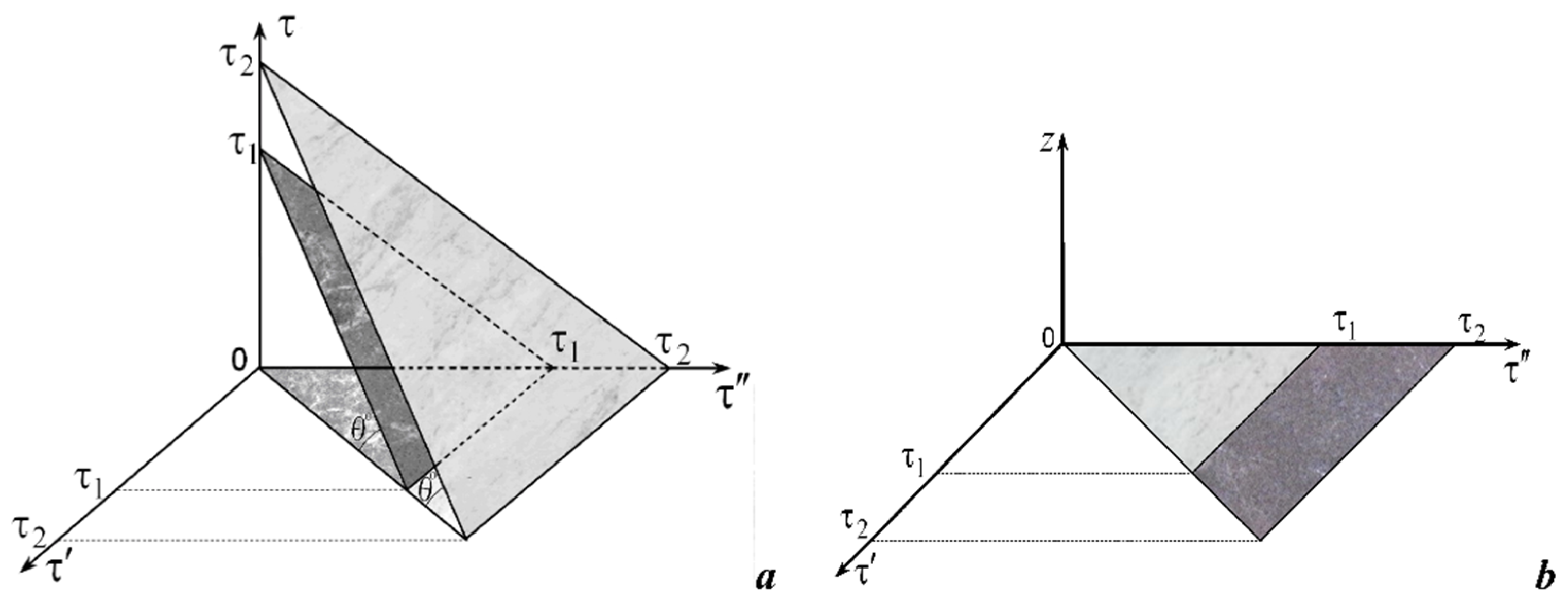
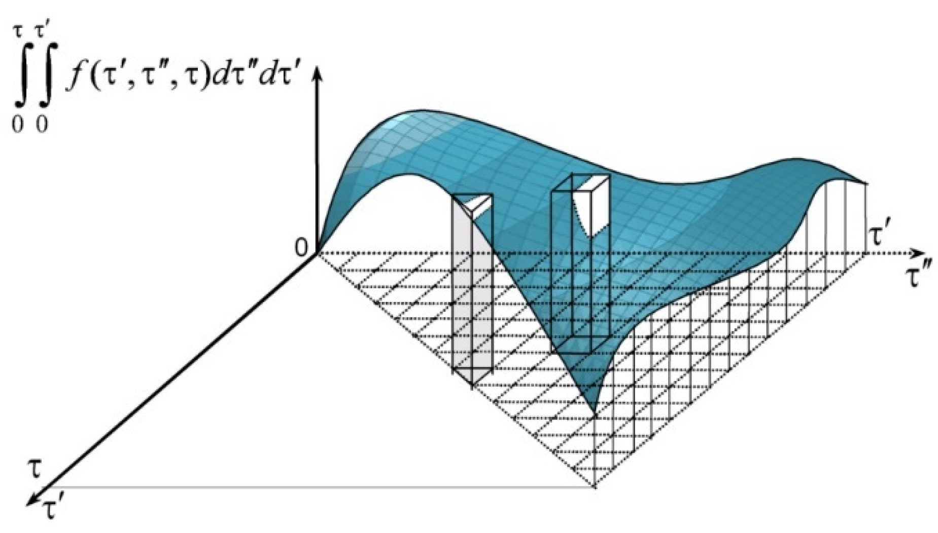
In the case of double integral with variable limits, it is not possible to estimate the calculation error by classical methods. Moreover, the variable limits of the integral

$$I(\mathsf{\tau })={\displaystyle \underset{0}{\overset{g_1(\mathsf{\tau })}{\int }}{\displaystyle \underset{0}{\overset{g_2({\mathsf{\tau }}^{\prime })}{\int }}f({\mathsf{\tau }}^{\prime },{\mathsf{\tau }}^{″},\mathsf{\tau })d{\mathsf{\tau }}^{″}d{\mathsf{\tau }}^{\prime }}}$$

(1)

are functions of independent variables τ, ${\mathsf{\tau }}^{\prime }$ $\in [0;\infty )$ that leads to variableness of the integration region.

We suppose that integral (1), functions f(τ′, τ″, τ), $g_1(\mathsf{\tau })$ and $g_2({\mathsf{\tau }}^{\prime })$ satisfy necessary restrictions (in particular, functions $g_1(\mathsf{\tau })$, $g_2({\mathsf{\tau }}^{\prime })$ are continuous functions of their arguments). Without loss of generality, we can accept that $g_1(\mathsf{\tau })=\mathsf{\tau }$ and $g_2({\mathsf{\tau }}^{\prime })={\mathsf{\tau }}^{\prime }$, because, if the inverse functions $g_1^{-1}(\mathsf{\tau })$ and $g_2^{-1}({\mathsf{\tau }}^{\prime })$ exist, then using change of variables $t=g_1(\mathsf{\tau })$ and $t^{\prime }=g_2({\mathsf{\tau }}^{\prime })$ the integral (1) can be reduced to the form

$$I(\mathsf{\tau })\equiv I\left(g_1^{-1}(t)\right)={\displaystyle \underset{0}{\overset{t}{\int }}{\displaystyle \underset{0}{\overset{t^{\prime }}{\int }}f(t^{\prime },{\mathsf{\tau }}^{″},t)\frac{\partial g_2^{-1}(t^{\prime })}{\partial t^{\prime }}d{\mathsf{\tau }}^{″}d{t}^{\prime }}}.$$

(2)

Note that zero values of the lower limits of integration can be obtained using the additive property of an integral.

2. Construction of Formula for Computing Double Integrals with Variable Upper Limits

A method of numerical integration of double integrals with variable upper limits, which we propose, may be divided into such steps:

• determination of integration region;
• overlaying square or rectangular grid on the integration region;
• decomposing of integration region into subregions, which consist of square (rectangular) and triangular elements;
• application of cubatures in the subdomain consisting of square elements;
• realization of triangulation division along the variable boundary τ″ = τ′;
• calculating the volumes of elementary elements based on triangles;
• calculation of the original integral;
• determination of calculation error.

2.1. Determination of Integration Region

The region of integration of the integrand (1) in the space $O\mathsf{\tau }{\mathsf{\tau }}^{\prime }{\mathsf{\tau }}^{″}$ has the form of an inclined triangle (Figure 1). Taking into account that τ is a variable, i.e., it changes continuously in $\Re$ or in the interval $[0;\infty )$ (for example, if τ is time) or in any closed interval, then with the change of τ the region of integration in space $O\mathsf{\tau }{\mathsf{\tau }}^{\prime }{\mathsf{\tau }}^{″}$ remains a triangle. The change of variable τ leads to a change in the maximum values of τ′ and τ″.

For τ = τ₁ we have max τ′ = max τ″= τ₁, and for τ = τ₂ we have max τ′ = max τ″ = τ₂ (Figure 1a). These regions are similar triangles that are in parallel planes, i.e., they are at the same angle θ to the plane Oτ′τ″ (Figure 1a). However, an area of the surface of integration changes. For τ = 0 the integration, the region is the point (0, 0, 0).

Let us make a projection of the surface of integration on the plane Oτ′τ″ (Figure 1b). Then we obtain the set of regions of integration in the space Oτ′τ″z.

As a result, we obtain a family of integrands parameterized by the variable τ (Figure 2).

2.2. Overlaying a Grid for the Variable Region of Integration

Let us overlay a square grid on the projection of the integration region (Figure 3a). Then we take into account the variableness of the integration region. Note, that with changes of value of τ either the number of division elements $N_{el}$ or the width of the grid (step) h can change, i.e., $N_{el}=N_{ei}(\mathsf{\tau })$, $h=h(\mathsf{\tau })$ and $h(\mathsf{\tau })=\frac{\mathsf{\tau }}{N_{el}(\mathsf{\tau })}$.

If we consider that the integration region S is a triangle, then with increasing τ from t₁ to t₂ the integration region remains a triangle, increases, and the area of the additional region $S_a$ increases by $S_a=\left(t_2^2-t_1^2\right)/2$ (Figure 3b). Then, if the grid for $\mathsf{\tau }=t_1$ ($N_{el}=N_{ei}(t_1)$, $h=h(t_1)$) is fixed, then at the same step h the number of division elements increases by $N_a=\frac{t_2-t_1}{h}$ elements. If we fix the number of division elements $N_{el}$, then with the changing τ from t₁ to t₂ there is a change in the width of the grid $h=\frac{t_2}{N_{el}}$. Note that the number of elements and the width of the grid can change together, and the relation $h{N}_{el}=t_2$ is always fulfilled.

At the same time, if necessary, the additional region $S_a$ can be divided with a different grid from the grid of the region S with the width $h_{t_2}=\frac{t_2-t_1}{N_a}$.

Analogous reasoning can be made for the rectangular grid, but we restrict ourselves to the case of the square grid.

2.3. Formula for Finding a Double Integral with Variable Upper Limits

We break up the integration region $S(\mathsf{\tau })$ into $N_{el}(\mathsf{\tau })$ small subregions. Then we apply the cubature formula with the weight function $w({\mathsf{\tau }}^{\prime },{\mathsf{\tau }}^{″})\equiv 1$. Depending on the number of division elements changes or the grid width changes when changing the variable τ we get the following cases.

(A)

With the change of τ, only the size of the imposed grid h(τ) changes

$${\displaystyle \underset{0}{\overset{\mathsf{\tau }}{\int }}{\displaystyle \underset{0}{\overset{{\mathsf{\tau }}^{\prime }}{\int }} f({\mathsf{\tau }}^{\prime },{\mathsf{\tau }}^{″},\mathsf{\tau })d{\mathsf{\tau }}^{″}d{\mathsf{\tau }}^{\prime }}}={\displaystyle \sum _{el}^{N_{el}}{\displaystyle \underset{\left(V_{el}(\mathsf{\tau })\right)}{\iint } f({\mathsf{\tau }}^{\prime },{\mathsf{\tau }}^{″},\mathsf{\tau })d{\mathsf{\tau }}^{″}d{\mathsf{\tau }}^{\prime }}},$$

(3)

(B)

With the change of τ, only the number of division elements N_el(τ) changes

$${\displaystyle \underset{0}{\overset{\mathsf{\tau }}{\int }}{\displaystyle \underset{0}{\overset{{\mathsf{\tau }}^{\prime }}{\int }} f({\mathsf{\tau }}^{\prime },{\mathsf{\tau }}^{″},\mathsf{\tau })d{\mathsf{\tau }}^{″}d{\mathsf{\tau }}^{\prime }}}={\displaystyle \sum _{el}^{N_{el}(\mathsf{\tau })}{\displaystyle \underset{\left(V_{el}\right)}{\iint } f({\mathsf{\tau }}^{\prime },{\mathsf{\tau }}^{″},\mathsf{\tau })d{\mathsf{\tau }}^{″}d{\mathsf{\tau }}^{\prime }}},$$

(4)

(C)

With the change of τ, both the size of the grid and the number of division elements change

$${\displaystyle \underset{0}{\overset{\mathsf{\tau }}{\int }}{\displaystyle \underset{0}{\overset{{\mathsf{\tau }}^{\prime }}{\int }} f({\mathsf{\tau }}^{\prime },{\mathsf{\tau }}^{″},\mathsf{\tau })d{\mathsf{\tau }}^{″}d{\mathsf{\tau }}^{\prime }}}={\displaystyle \sum _{el}^{N_{el}(\mathsf{\tau })}{\displaystyle \underset{\left(V_{el}(\mathsf{\tau })\right)}{\iint } f({\mathsf{\tau }}^{\prime },{\mathsf{\tau }}^{″},\mathsf{\tau })d{\mathsf{\tau }}^{″}d{\mathsf{\tau }}^{\prime }}},$$

(5)

where V_el is the volume of the individual element of division of the integration region.

As a result of the division of the integration region, we obtained square (Figure 4a) and triangular (Figure 4b) elements. Here the summation is carried out over all elements ${\displaystyle \underset{el}{\cup }{V}_{el}=[0, {\mathsf{\tau }}^{\prime }]\times [0, \mathsf{\tau }]}$.

We separate square and triangular elements:

$$(\mathrm{A}) {\displaystyle \sum _{el}^{N_{el}}{\displaystyle \underset{\left(V_{el}(\mathsf{\tau })\right)}{\iint }f({\mathsf{\tau }}^{\prime },{\mathsf{\tau }}^{″},\mathsf{\tau })d{\mathsf{\tau }}^{″}d{\mathsf{\tau }}^{\prime }}}={\displaystyle \sum _{s{q}_{el}}^{N_{s{q}_{el}}}{\displaystyle \underset{\left(V_{s{q}_{el}}(\mathsf{\tau })\right)}{\iint } f({\mathsf{\tau }}^{\prime },{\mathsf{\tau }}^{″},\mathsf{\tau })d{\mathsf{\tau }}^{″}d{\mathsf{\tau }}^{\prime }}}+{\displaystyle \sum _{{tr}_{el}}^{N_{t{r}_{el}}}{\displaystyle \underset{\left(V_{{tr}_{el}}(\mathsf{\tau })\right)}{\iint } f({\mathsf{\tau }}^{\prime },{\mathsf{\tau }}^{″},\mathsf{\tau })d{\mathsf{\tau }}^{″}d{\mathsf{\tau }}^{\prime }}},$$

(6)

$$(\mathrm{B}) {\displaystyle \sum _{el}^{N_{el}(\mathsf{\tau })}{\displaystyle \underset{\left(V_{el}\right)}{\iint }f({\mathsf{\tau }}^{\prime },{\mathsf{\tau }}^{″},\mathsf{\tau })d{\mathsf{\tau }}^{″}d{\mathsf{\tau }}^{\prime }}}={\displaystyle \sum _{s{q}_{el}}^{N_{s{q}_{el}}(\mathsf{\tau })}{\displaystyle \underset{\left(V_{s{q}_{el}}\right)}{\iint } f({\mathsf{\tau }}^{\prime },{\mathsf{\tau }}^{″},\mathsf{\tau })d{\mathsf{\tau }}^{″}d{\mathsf{\tau }}^{\prime }}}+{\displaystyle \sum _{{tr}_{el}}^{N_{t{r}_{el}}(\mathsf{\tau })}{\displaystyle \underset{\left(V_{{tr}_{el}}\right)}{\iint } f({\mathsf{\tau }}^{\prime },{\mathsf{\tau }}^{″},\mathsf{\tau })d{\mathsf{\tau }}^{″}d{\mathsf{\tau }}^{\prime }}},$$

(7)

$$(\mathrm{C}) {\displaystyle \sum _{el}^{N_{el}(\mathsf{\tau })}{\displaystyle \underset{\left(V_{el}(\mathsf{\tau })\right)}{\iint }f({\mathsf{\tau }}^{\prime },{\mathsf{\tau }}^{″},\mathsf{\tau })d{\mathsf{\tau }}^{″}d{\mathsf{\tau }}^{\prime }}}={\displaystyle \sum _{s{q}_{el}}^{N_{s{q}_{el}}(\mathsf{\tau })}{\displaystyle \underset{\left(V_{s{q}_{el}}(\mathsf{\tau })\right)}{\iint } f({\mathsf{\tau }}^{\prime },{\mathsf{\tau }}^{″},\mathsf{\tau })d{\mathsf{\tau }}^{″}d{\mathsf{\tau }}^{\prime }}}+{\displaystyle \sum _{{tr}_{el}}^{N_{t{r}_{el}}(\mathsf{\tau })}{\displaystyle \underset{\left(V_{{tr}_{el}}(\mathsf{\tau })\right)}{\iint } f({\mathsf{\tau }}^{\prime },{\mathsf{\tau }}^{″},\mathsf{\tau })d{\mathsf{\tau }}^{″}d{\mathsf{\tau }}^{\prime }}},$$

(8)

where sq_el is the square element, tr_el is the triangular element, $N_{s{q}_{el}}$ and $N_{t{r}_{el}}$ are the numbers of square and triangular elements, $V_{s{q}_{el}}$ and $V_{t{r}_{el}}$ are the volumes of square and triangular elements,

Let us select the elements V_el, which are squares (Figure 4a). Here we apply numerical integration in cubatures. So, we have

$$(\mathrm{A}) {\displaystyle \underset{{\displaystyle \underset{{sq}_{el}}{\cup }{V}_{el}(\mathsf{\tau })}}{\iint } f({\mathsf{\tau }}^{\prime },{\mathsf{\tau }}^{″},\mathsf{\tau })d{\mathsf{\tau }}^{″}d{\mathsf{\tau }}^{\prime }}={\displaystyle \sum _{s{q}_{el}}^{N_{s{q}_{el}}}{\displaystyle \underset{\left(V_{s{q}_{el}}(\mathsf{\tau })\right)}{\iint } f({\mathsf{\tau }}^{\prime },{\mathsf{\tau }}^{″},\mathsf{\tau })d{\mathsf{\tau }}^{″}d{\mathsf{\tau }}^{\prime }}}={\displaystyle \sum _{i=1}^{n-1}{\displaystyle \sum _{j=i+1}^n{h}^2(\mathsf{\tau }) f({{\mathsf{\tau }}^{\prime }}_i,{{\mathsf{\tau }}^{″}}_j,\mathsf{\tau })}},$$

(9)

$n\equiv const$, $n\in {\rm N}$, $n-1$ is the number of square elements in the longest line, h(τ) is the grid width depending on τ.

$$(\mathrm{B}) {\displaystyle \underset{{\displaystyle \underset{{sq}_{el}(\mathsf{\tau })}{\cup }{V}_{el}}}{\iint } f({\mathsf{\tau }}^{\prime },{\mathsf{\tau }}^{″},\mathsf{\tau })d{\mathsf{\tau }}^{″}d{\mathsf{\tau }}^{\prime }}={\displaystyle \sum _{s{q}_{el}}^{N_{s{q}_{el}}(\mathsf{\tau })}{\displaystyle \underset{\left(V_{s{q}_{el}}\right)}{\iint } f({\mathsf{\tau }}^{\prime },{\mathsf{\tau }}^{″},\mathsf{\tau })d{\mathsf{\tau }}^{″}d{\mathsf{\tau }}^{\prime }}})={\displaystyle \sum _{i=1}^{n(\mathsf{\tau })-1}{\displaystyle \sum _{j=i+1}^{n(\mathsf{\tau })}{h}^2 f({{\mathsf{\tau }}^{\prime }}_i,{{\mathsf{\tau }}^{″}}_j,\mathsf{\tau })}},$$

(10)

$h\equiv const$, n(τ) changes with changing τ.

$$(\mathrm{C}) {\displaystyle \underset{{\displaystyle \underset{{sq}_{el}(\mathsf{\tau })}{\cup }{V}_{el}(\mathsf{\tau })}}{\iint } f({\mathsf{\tau }}^{\prime },{\mathsf{\tau }}^{″},\mathsf{\tau })d{\mathsf{\tau }}^{″}d{\mathsf{\tau }}^{\prime }}={\displaystyle \sum _{s{q}_{el}}^{N_{s{q}_{el}}(\mathsf{\tau })}{\displaystyle \underset{\left(V_{s{q}_{el}}(\mathsf{\tau })\right)}{\iint } f({\mathsf{\tau }}^{\prime },{\mathsf{\tau }}^{″},\mathsf{\tau })d{\mathsf{\tau }}^{″}d{\mathsf{\tau }}^{\prime }}}={\displaystyle \sum _{i=1}^{n(\mathsf{\tau })-1}{\displaystyle \sum _{j=i+1}^{n(\mathsf{\tau })}{h}^2(\mathsf{\tau }) f({{\mathsf{\tau }}^{\prime }}_i,{{\mathsf{\tau }}^{″}}_j,\mathsf{\tau })}},$$

(11)

n(τ) and h(τ) change with changing τ.

Note that h(τ) = τ/n(τ).

Consider the subregion consisting of triangles only (Figure 4b). The sum of the volumes of the elements with a triangular base takes the form

$$(\mathrm{A}) {\displaystyle \sum _{{tr}_{el}}^{}{\displaystyle \underset{\left(V_{{tr}_{el}}(\mathsf{\tau })\right)}{\iint } f({\mathsf{\tau }}^{\prime },{\mathsf{\tau }}^{″},\mathsf{\tau })d{\mathsf{\tau }}^{″}d{\mathsf{\tau }}^{\prime }}}={\displaystyle \sum _{i=1}^n{h}^2(\mathsf{\tau })f({{\mathsf{\tau }}^{\prime }}_i,{{\mathsf{\tau }}^{″}}_i,\mathsf{\tau })},$$

(12)

$$(\mathrm{B}) {\displaystyle \sum _{{tr}_{el}(\mathsf{\tau })}^{}{\displaystyle \underset{\left(V_{{tr}_{el}}\right)}{\iint } f({\mathsf{\tau }}^{\prime },{\mathsf{\tau }}^{″},\mathsf{\tau })d{\mathsf{\tau }}^{″}d{\mathsf{\tau }}^{\prime }}}={\displaystyle \sum _{i=1}^{n(\mathsf{\tau })}{h}^{2}f({{\mathsf{\tau }}^{\prime }}_i,{{\mathsf{\tau }}^{″}}_i,\mathsf{\tau })},$$

(13)

$$(\mathrm{C}) {\displaystyle \sum _{{tr}_{el}(\mathsf{\tau })}^{}{\displaystyle \underset{\left(V_{{tr}_{el}}(\mathsf{\tau })\right)}{\iint } f({\mathsf{\tau }}^{\prime },{\mathsf{\tau }}^{″},\mathsf{\tau })d{\mathsf{\tau }}^{″}d{\mathsf{\tau }}^{\prime }}}={\displaystyle \sum _{i=1}^{n(\mathsf{\tau })}{h}^2(\mathsf{\tau })f({{\mathsf{\tau }}^{\prime }}_i,{{\mathsf{\tau }}^{″}}_i,\mathsf{\tau })},$$

(14)

where n is the number of triangular elements; ${{\mathsf{\tau }}^{\prime }}_{i+1}={{\mathsf{\tau }}^{\prime }}_i+h(\mathsf{\tau })$; ${{\mathsf{\tau }}^{\prime }}_i$ and ${{\mathsf{\tau }}^{″}}_i$ are the values of τ′ and τ″ in the ith node (the i-th triangular elements).

Note that the number of triangular elements is 1 more than the square elements in the longest line.

By Formulas (6)–(8), we sum the relations (9)–(11) and (12)–(14) respectively. Then we obtain the formulas of numerical integration for a double integral with variable upper limits:

$$(\mathrm{A}) {\displaystyle \underset{0}{\overset{\mathsf{\tau }}{\int }}{\displaystyle \underset{0}{\overset{{\mathsf{\tau }}^{\prime }}{\int }}f({\mathsf{\tau }}^{\prime },{\mathsf{\tau }}^{″},\mathsf{\tau })}dxdy}\approx \left(\frac{1}{2}{\displaystyle \sum _{i=1}^n{h}^2(\mathsf{\tau }) f({{\mathsf{\tau }}^{\prime }}_i,{{\mathsf{\tau }}^{″}}_i,\mathsf{\tau })}+{\displaystyle \sum _{i=1}^{n-1}{\displaystyle \sum _{j=i+1}^n{h}^2(\mathsf{\tau }) f({{\mathsf{\tau }}^{\prime }}_i,{{\mathsf{\tau }}^{″}}_j,\mathsf{\tau })}}\right),$$

(15)

$$(\mathrm{B}) {\displaystyle \underset{0}{\overset{\mathsf{\tau }}{\int }}{\displaystyle \underset{0}{\overset{{\mathsf{\tau }}^{\prime }}{\int }}f({\mathsf{\tau }}^{\prime },{\mathsf{\tau }}^{″},\mathsf{\tau })}dxdy}\approx \left(\frac{1}{2}{\displaystyle \sum _{i=1}^{n(\mathsf{\tau })}{h}^2 f({{\mathsf{\tau }}^{\prime }}_i,{{\mathsf{\tau }}^{″}}_i,\mathsf{\tau })}+{\displaystyle \sum _{i=1}^{n(\mathsf{\tau })-1}{\displaystyle \sum _{j=i+1}^{n(\mathsf{\tau })}{h}^2 f({{\mathsf{\tau }}^{\prime }}_i,{{\mathsf{\tau }}^{″}}_j,\mathsf{\tau })}}\right),$$

(16)

$$(\mathrm{C}) {\displaystyle \underset{0}{\overset{\mathsf{\tau }}{\int }}{\displaystyle \underset{0}{\overset{{\mathsf{\tau }}^{\prime }}{\int }}f({\mathsf{\tau }}^{\prime },{\mathsf{\tau }}^{″},\mathsf{\tau })}dxdy}\approx \left(\frac{1}{2}{\displaystyle \sum _{i=1}^{n(\mathsf{\tau })}{h}^2(\mathsf{\tau }) f({{\mathsf{\tau }}^{\prime }}_i,{{\mathsf{\tau }}^{″}}_i,\mathsf{\tau })}+{\displaystyle \sum _{i=1}^{n(\mathsf{\tau })-1}{\displaystyle \sum _{j=i+1}^{n(\mathsf{\tau })}{h}^2(\mathsf{\tau }) f({{\mathsf{\tau }}^{\prime }}_i,{{\mathsf{\tau }}^{″}}_j,\mathsf{\tau })}}\right),$$

(17)

where ${{\mathsf{\tau }}^{\prime }}_{i+1}={{\mathsf{\tau }}^{\prime }}_i+h(\mathsf{\tau })$; ${{\mathsf{\tau }}^{″}}_{i+1}={{\mathsf{\tau }}^{″}}_i+h(\mathsf{\tau })$.

Schematically, such a method of numerical integration for a double integral with variable upper limits at a fixed value of τ is presented in Figure 5.

3. Error of Numerical Integration

We find the error of numerical integration by the Taylor formula [34,35].

The main term of the error is [36,37].

$$R(\mathsf{\tau })={\displaystyle \underset{0}{\overset{\mathsf{\tau }}{\int }}{\displaystyle \underset{0}{\overset{{\mathsf{\tau }}^{\prime }}{\int }}f(\mathsf{\tau },{{\mathsf{\tau }}^{\prime }}_{},{{\mathsf{\tau }}^{″}}_{})d{\mathsf{\tau }}^{″}d{\mathsf{\tau }}^{\prime }-S(\mathsf{\tau })·f(\mathsf{\tau },{{\mathsf{\tau }}^{\prime }}_c,{{\mathsf{\tau }}^{″}}_c)}},$$

(18)

where $S(\mathsf{\tau })$ is the area of the region of integration, $({{\mathsf{\tau }}^{\prime }}_c,{{\mathsf{\tau }}^{″}}_c)$ is the central point of the region of integration.

We choose the central point of the integration region $({{\mathsf{\tau }}^{\prime }}_c,{{\mathsf{\tau }}^{″}}_c)$ in the vicinity of which we expand the function

$$F(\mathsf{\tau },{\mathsf{\tau }}^{\prime },{\mathsf{\tau }}^{″})={\displaystyle \underset{0}{\overset{\mathsf{\tau }}{\int }}{\displaystyle \underset{0}{\overset{{\mathsf{\tau }}^{\prime }}{\int }}f(\mathsf{\tau },{\mathsf{\tau }}^{\prime },{\mathsf{\tau }}^{″})d{\mathsf{\tau }}^{″}d{\mathsf{\tau }}^{\prime }}}$$

into the Taylor series

$$F(\mathsf{\tau },{\mathsf{\tau }}^{\prime },{\mathsf{\tau }}^{″})=F(\mathsf{\tau },{{\mathsf{\tau }}^{\prime }}_c,{{\mathsf{\tau }}^{″}}_c)+({\mathsf{\tau }}^{\prime }-{{\mathsf{\tau }}^{\prime }}_c){F^{\prime }}_{{\mathsf{\tau }}^{\prime }}(\mathsf{\tau },{{\mathsf{\tau }}^{\prime }}_c,{{\mathsf{\tau }}^{″}}_c)+({\mathsf{\tau }}^{″}-{{\mathsf{\tau }}^{″}}_c){F^{\prime }}_{{\mathsf{\tau }}^{″}}(\mathsf{\tau },{{\mathsf{\tau }}^{\prime }}_c,{{\mathsf{\tau }}^{″}}_c)+\dots .$$

Note that the function F(τ, τ′, τ″) can be expanded into a Taylor series if in some vicinity of the point $({{\mathsf{\tau }}^{\prime }}_c,{{\mathsf{\tau }}^{″}}_c)$ its continuous partial derivatives exist up to $n+1$ order [38].

Let f(τ, τ′, τ″) be continuous in the domain $[0,\mathsf{\tau }]\times [0,\mathsf{\tau }]$. Then it is integrated into this domain, as well as integrated into any subdomain of $[0,\mathsf{\tau }]\times [0,{\mathsf{\tau }}^{\prime }]$ [38]. Then F(τ, τ′, τ″) is continuous in the domain $[0,\mathsf{\tau }]\times [0,\mathsf{\tau }]$. If f(τ, τ′, τ″) is continuous in the domain $[0,\mathsf{\tau }]\times [0,\mathsf{\tau }]$ then F(τ, τ′, τ″) is differentiable in the domain $[0,\mathsf{\tau }]\times [0,\mathsf{\tau }]$ [38].

Taking into consideration that F(τ, τ′, τ″) is the double integral with variable upper limits, we obtain (by the analogy of double integration in cubatures)

$$\begin{gathered} F(\mathsf{\tau },{{\mathsf{\tau }}^{\prime }}_c,{{\mathsf{\tau }}^{″}}_c)={\displaystyle \underset{0}{\overset{\mathsf{\tau }}{\int }}{\displaystyle \underset{0}{\overset{{{\mathsf{\tau }}^{\prime }}_c}{\int }}f(\mathsf{\tau },{{\mathsf{\tau }}^{\prime }}_c,{{\mathsf{\tau }}^{″}}_c)}}d{{\mathsf{\tau }}^{\prime }}^{\prime }d{\mathsf{\tau }}^{\prime }=f(\mathsf{\tau },{{\mathsf{\tau }}^{\prime }}_c,{{\mathsf{\tau }}^{″}}_c){\displaystyle \underset{0}{\overset{\mathsf{\tau }}{\int }}{\displaystyle \underset{0}{\overset{{{\mathsf{\tau }}^{\prime }}_c}{\int }}d{{\mathsf{\tau }}^{\prime }}^{\prime }d{\mathsf{\tau }}^{\prime }=f(\mathsf{\tau },{{\mathsf{\tau }}^{\prime }}_c,{{\mathsf{\tau }}^{″}}_c)\mathsf{\tau }}}{{\mathsf{\tau }}^{\prime }}_c; \\ {F^{\prime }}_{{\mathsf{\tau }}^{\prime }}(\mathsf{\tau },{{\mathsf{\tau }}^{\prime }}_c,{{\mathsf{\tau }}^{″}}_c)={\displaystyle \underset{0}{\overset{\mathsf{\tau }}{\int }}{\displaystyle \underset{0}{\overset{{{\mathsf{\tau }}^{\prime }}_c}{\int }}{{f^{\prime }}_{{\mathsf{\tau }}^{\prime }}(\mathsf{\tau },{{\mathsf{\tau }}^{\prime }}_{},{{\mathsf{\tau }}^{″}}_c)|}_{{\mathsf{\tau }}^{\prime }={{\mathsf{\tau }}^{\prime }}_c}}}d{{\mathsf{\tau }}^{\prime }}^{\prime }d{\mathsf{\tau }}^{\prime }={\displaystyle \underset{0}{\overset{\mathsf{\tau }}{\int }}f(\mathsf{\tau },{{\mathsf{\tau }}^{\prime }}_c,{{\mathsf{\tau }}^{″}}_c)}d{\mathsf{\tau }}^{\prime }=f(\mathsf{\tau },{{\mathsf{\tau }}^{\prime }}_c,{{\mathsf{\tau }}^{″}}_c)\mathsf{\tau }; \\ {F^{\prime }}_{{\mathsf{\tau }}^{″}}(\mathsf{\tau },{{\mathsf{\tau }}^{\prime }}_c,{{\mathsf{\tau }}^{″}}_c)={\displaystyle \underset{0}{\overset{\mathsf{\tau }}{\int }}{\displaystyle \underset{0}{\overset{{{\mathsf{\tau }}^{\prime }}_c}{\int }}{{f^{\prime }}_{{\mathsf{\tau }}^{″}}(\mathsf{\tau },{{\mathsf{\tau }}^{\prime }}_c,{{\mathsf{\tau }}^{″}}_{})|}_{{\mathsf{\tau }}^{″}={{\mathsf{\tau }}^{″}}_c}}}d{{\mathsf{\tau }}^{\prime }}^{\prime }d{\mathsf{\tau }}^{″}={{f^{\prime }}_{{\mathsf{\tau }}^{″}}(\mathsf{\tau },{{\mathsf{\tau }}^{\prime }}_c,{{\mathsf{\tau }}^{″}}_c)|}_{{\mathsf{\tau }}^{″}={{\mathsf{\tau }}^{″}}_c}\mathsf{\tau }{{\mathsf{\tau }}^{\prime }}_c; \\ \dots \end{gathered}$$

Here we have used Barrow’s theorem [38]

$${\left({\displaystyle \underset{a}{\overset{t}{\int }}f(}x)dx\right)}^{\prime }=f(t).$$

Note that as distinct from double integrating within the definite limits, the first derivatives do not disappear and must be taken into account. We include them in error.

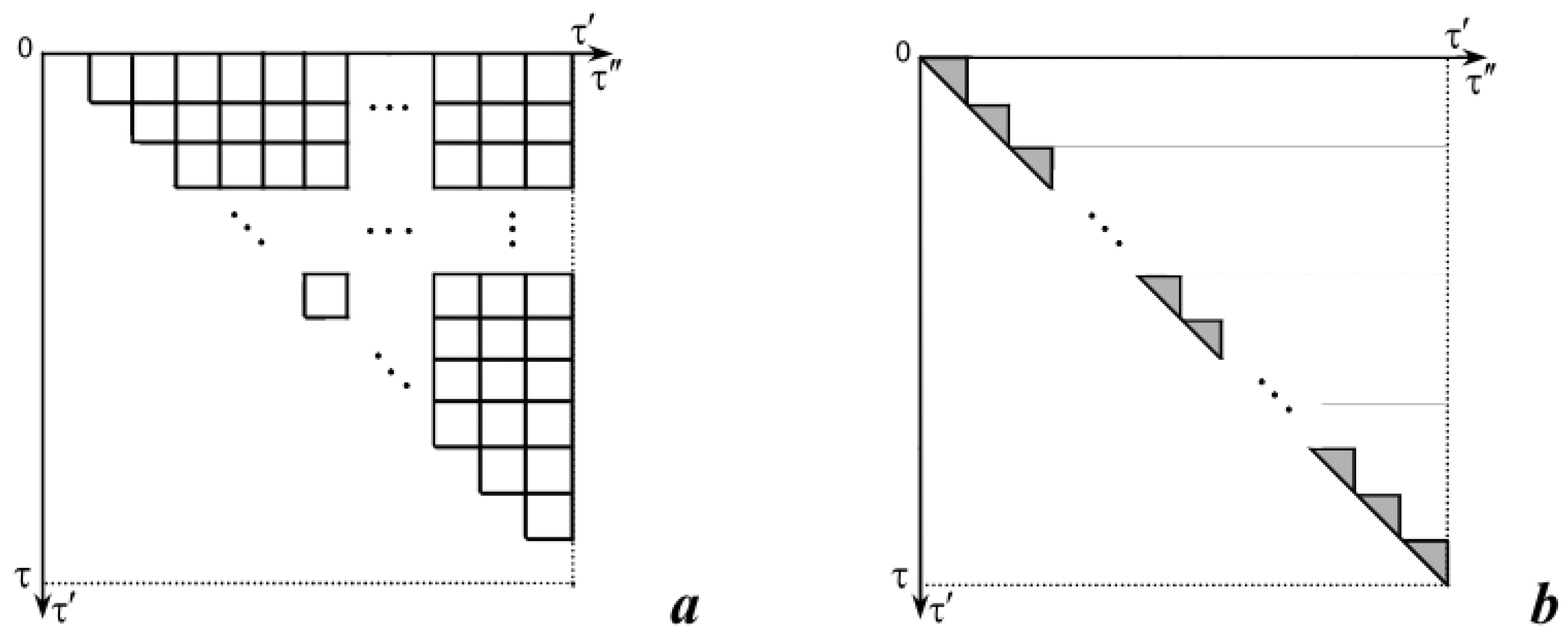
We will write down separately the errors for triangular and square elements. The integration error (18) for each triangular element takes the form

$$R_i(\mathsf{\tau })=1/2S_{{tr}_{el}i}(\mathsf{\tau })\left(h(\mathsf{\tau }){F^{\prime }}_{{\mathsf{\tau }}^{\prime }}(\mathsf{\tau },{{\mathsf{\tau }}^{\prime }}_c,{{\mathsf{\tau }}^{″}}_c)+h(\mathsf{\tau }){F^{\prime }}_{{\mathsf{\tau }}^{″}}(\mathsf{\tau },{{\mathsf{\tau }}^{\prime }}_c,{{\mathsf{\tau }}^{″}}_c)\right) (i=\overline{1,n(\mathsf{\tau })}).$$

(19)

The error of integration (18) for each square element is

$$\begin{gathered} R_{ij}(\mathsf{\tau })=1/24S_{s{q}_{el}ij}(\mathsf{\tau })\left(h_{}^2(\mathsf{\tau }){F^{″}}_{{\mathsf{\tau }}^{\prime }{\mathsf{\tau }}^{\prime }}(\mathsf{\tau },{{\mathsf{\tau }}^{\prime }}_c,{{\mathsf{\tau }}^{″}}_c)+h_{}^2(\mathsf{\tau }){F^{″}}_{{\mathsf{\tau }}^{″}{\mathsf{\tau }}^{″}}(\mathsf{\tau },{{\mathsf{\tau }}^{\prime }}_c,{{\mathsf{\tau }}^{″}}_c)\right) \\ (i=\overline{1,n(\mathsf{\tau })-1}, j=\overline{i+1,n(\mathsf{\tau })}). \end{gathered}$$

(20)

Here $S_{{tr}_{el}i}(\mathsf{\tau })$ and $S_{s{q}_{el}ij}(\mathsf{\tau })$ are areas of the ith triangular element and the ijth square element accordingly.

Summing the expressions (19) and (20) for the region in which the integral is defined, we obtain the error of our method

$$\begin{gathered} R(\mathsf{\tau })\approx \frac{h(\mathsf{\tau })}{2}\left({\displaystyle \underset{\left(V_{qua{d}_{el}}(\mathsf{\tau })\right)}{\iint } {F^{\prime }}_{{\mathsf{\tau }}^{\prime }}(\mathsf{\tau },{\mathsf{\tau }}^{\prime },{\mathsf{\tau }}^{″})d{\mathsf{\tau }}^{\prime }d{\mathsf{\tau }}^{″}}+{\displaystyle \underset{\left(V_{qua{d}_{el}}(\mathsf{\tau })\right)}{\iint } {F^{\prime }}_{{\mathsf{\tau }}^{″}}(\mathsf{\tau },{\mathsf{\tau }}^{\prime },{\mathsf{\tau }}^{″})d{\mathsf{\tau }}^{\prime }d{\mathsf{\tau }}^{″}}\right) \\ +\frac{h^2(\mathsf{\tau })}{24}\left({\displaystyle \underset{\left(V_{{\mathrm{triangular}}_{el}}(\mathsf{\tau })\right)}{\iint }{F^{″}}_{{\mathsf{\tau }}^{\prime }{\mathsf{\tau }}^{\prime }}(\mathsf{\tau },{\mathsf{\tau }}^{\prime },{\mathsf{\tau }}^{″})d{\mathsf{\tau }}^{\prime }d{\mathsf{\tau }}^{″}}+{\displaystyle \underset{\left(V_{{\mathrm{triangular}}_{el}}(\mathsf{\tau })\right)}{\iint }{F^{″}}_{{\mathsf{\tau }}^{″}{\mathsf{\tau }}^{″}}(\mathsf{\tau },{\mathsf{\tau }}^{\prime },{\mathsf{\tau }}^{″})d{\mathsf{\tau }}^{\prime }d{\mathsf{\tau }}^{″}}\right) \end{gathered}$$

(21)

or

$$R(\mathsf{\tau })=O(2h(\mathsf{\tau })+2h^2(\mathsf{\tau }))=O(2h(\mathsf{\tau })).$$

Since higher degrees of h(τ) are rejected in the estimates (19) and (20), the relation for the error (21) is asymptotic, and it is satisfied at h(τ)→0 with an accuracy to the terms of a higher order of smallness than h(τ).

If we impose the definite limits of integration, the obtained Formula (21) is reduced to the classical formula for the error by the expansion of an integrand into the Taylor series and estimation of the error of the method takes the form $R(\mathsf{\tau })=O(2h^2(\mathsf{\tau }))$.

4. Examples of Numerical Integration for the Double Integral with Variable Upper Limits

To test the efficiency and reliability of the obtained formulas of the numerical method, we apply it to the integration of sufficiently simple functions for which the integration expression can be found analytically.

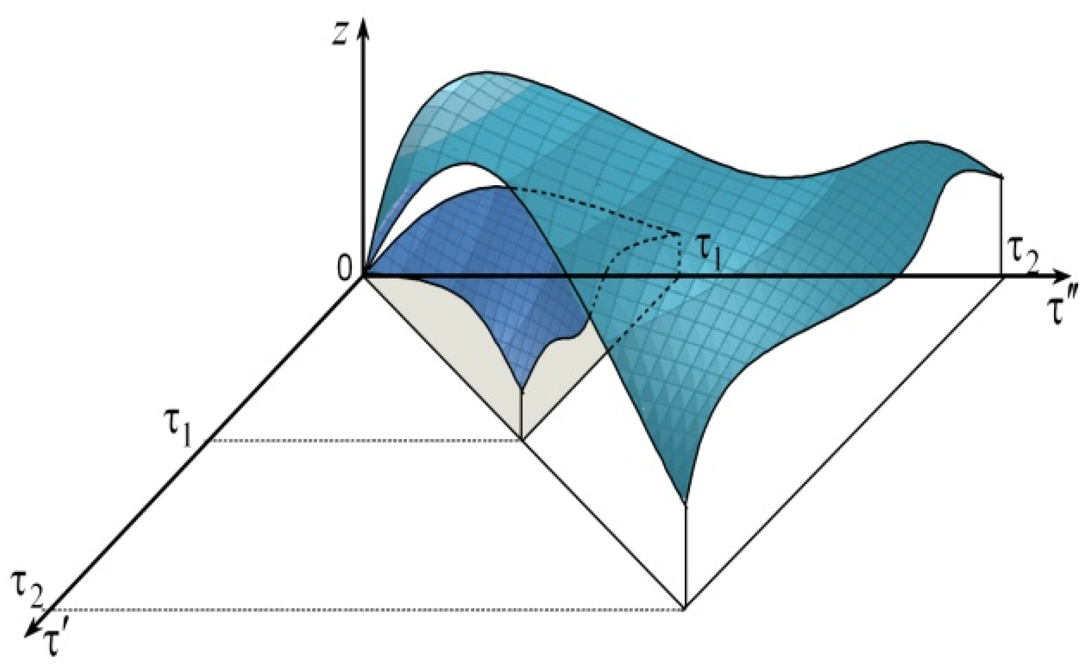
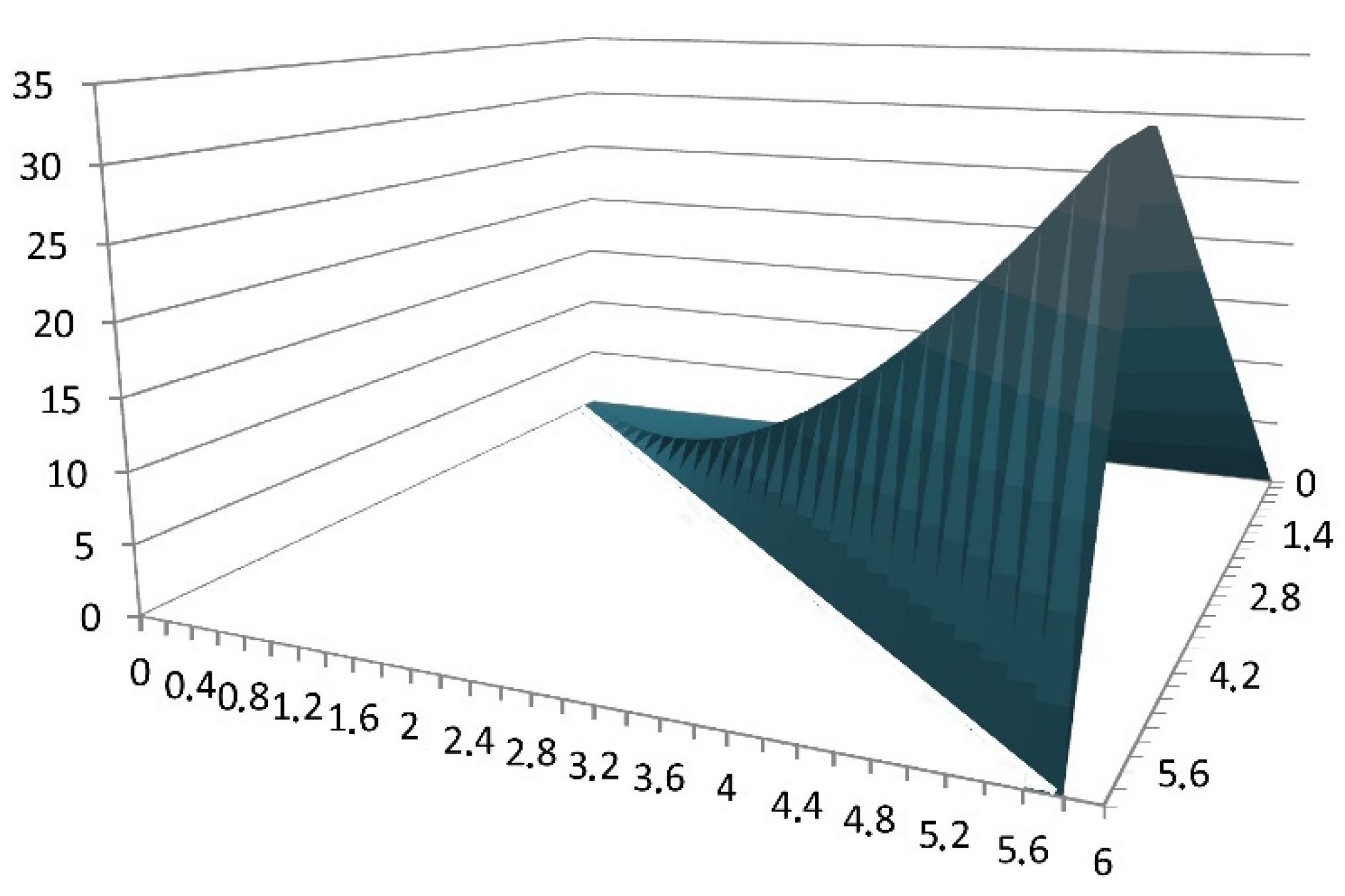
I. Let such an integrand be given f(τ′, τ″) = τ′τ″. The surface formed by the function f(τ′, τ″) over the integration region is shown in Figure 6.

Then we calculate the integral $I_{num}=$ ${\displaystyle \underset{0}{\overset{\mathsf{\tau }}{\int }}{\displaystyle \underset{0}{\overset{{\mathsf{\tau }}^{\prime }}{\int }}{\mathsf{\tau }}^{\prime }{\mathsf{\tau }}^{″}d{\mathsf{\tau }}^{\prime }d{\mathsf{\tau }}^{″}}}$ by Formulas (15)–(17) depending on the number of division elements changes and the grid width and analytically, namely $I_{analyt}=$ $\frac{1}{8}\mathsf{\tau }$.

The results of calculations are shown in

Table 1. Calculation of integral ${\displaystyle \underset{0}{\overset{\mathsf{\tau }}{\int }}{\displaystyle \underset{0}{\overset{{\mathsf{\tau }}^{\prime }}{\int }}{\mathsf{\tau }}^{\prime }{\mathsf{\tau }}^{″}d{\mathsf{\tau }}^{\prime }d{\mathsf{\tau }}^{″}}}$ for the case of A.

n(τ)	h(τ)	τ	${\mathit{V}}_{\mathit{s}{\mathit{q}}_{\mathit{e}\mathit{l}}}$	${\mathit{V}}_{\mathit{t}{\mathit{r}}_{\mathit{e}\mathit{l}}}$	Ianalyt	Inum	|Ianalyt − Inum|	E(τ)
104	0.0001	1	0.124983331	0.000016667	0.125	0.124999998	2 × 10−9	1.999999992 × 10−8
104	0.0002	2	1.999733293	0.000266667	2	1.99999996	4 × 10−8	1.999999992 × 10−8
104	0.0003	3	10.123649798	0.00135	10.125	10.124999798	2.03 × 10−7	2.000000004 × 10−8
104	0.0004	4	31.995732693	0.004266667	32	31.99999936	6.4 × 10−7	1.999999992 × 10−8
104	0.0005	5	78.114581771	0.010416667	78.125	78.124998438	1.562 × 10−6	1.999999987 × 10−8
104	0.0006	6	161.97839676	0.0216	162	161.99999676	3.24 × 10−6	2.000000004 × 10−8
104	0.0007	7	300.084977331	0.040016667	300.125	300.124993998	6.002 × 10−6	1.999999967 × 10−8
104	0.0008	8	511.931723094	0.068266666	512	511.99998976	1.024 × 10−5	1.999999992 × 10−8
104	0.0009	9	820.015633598	0.109350000	820.125	820.124983598	1.6402 × 10−5	1.999999987 × 10−8
104	0.001	10	1249.833308334	0.166666666	1250	1249.999975	2.5 × 10−5	1.999999987 × 10−8
104	0.0011	11	1829.880946731	0.244016666	1830.125	1830.12496339	3.6603 × 10−5	2.000000001 × 10−8
104	0.0012	12	2591.654348161	0.345599999	2592	2591.99994816	5.184 × 10−5	2.000000004 × 10−8
104	0.0013	13	3569.648911932	0.476016665	3570.125	3570.12492859	7.1402 × 10−5	1.999999996 × 10−8
104	0.0014	14	4801.359637295	0.640266665	4802	4801.99990396	9.604 × 10−5	1.999999967 × 10−8
104	0.0015	15	6327.28112344	0.843749998	6328.125	6328.12487343	1.26562 × 10−4	1.999999974 × 10−8
104	0.0016	16	8190.907569496	1.092266664	8192	8191.99983616	1.6384 × 10−4	1.999999992 × 10−8
104	0.0017	17	1.0438732774534 × 104	1.392016663	1.044 × 104	1.0440124791 × 104	2.08803 × 10−4	2.000000001 × 10−8
104	0.0018	18	1.3120250137564 × 104	1.749599996	13122	1.3121999737 × 104	2.6244 × 10−4	1.999999987 × 10−8
104	0.0019	19	1.6287952657536 × 104	2.172016661	1.629 × 104	1.6290124674 × 104	3.25802 × 10−4	1.999999984 × 10−8
104	0.002	20	1.9997332933340 × 104	2.666666660	2 × 104	1.99999996 × 104	4 × 10−4	1.999999987 × 10−8

,

Table 2. Calculation of integral ${\displaystyle \underset{0}{\overset{\mathsf{\tau }}{\int }}{\displaystyle \underset{0}{\overset{{\mathsf{\tau }}^{\prime }}{\int }}{\mathsf{\tau }}^{\prime }{\mathsf{\tau }}^{″}d{\mathsf{\tau }}^{\prime }d{\mathsf{\tau }}^{″}}}$ for the case B.

n(τ)	h(τ)	τ	${\mathit{V}}_{\mathit{s}{\mathit{q}}_{\mathit{e}\mathit{l}}}$	${\mathit{V}}_{\mathit{t}{\mathit{r}}_{\mathit{e}\mathit{l}}}$	Ianalyt	Inum	|Ianalyt − Inum|	E(τ)
104	0.0001	1	0.124983331	1.67 × 10−5	0.125	0.124999998	2.5 × 10−9	2 × 10−8
2 × 104	0.0001	2	1.999866657	0.000133333	2	1.99999999	10−8	5 × 10−9
3 × 104	0.0001	3	10.12454998	0.00045	10.125	10.12499998	2.25 × 10−8	2.2222 × 10−9
4 × 104	0.0001	4	31.99893329	0.001066667	32	31.99999996	4 × 10−8	1.25 × 10−9
5 × 104	0.0001	5	78.1229166	0.002083333	78.125	78.12499994	6.25 × 10−8	8 × 10−9
6 × 104	0.0001	6	161.9963999	0.0036	162	161.9999999	9.00002 × 10−8	5.5556 × 10−10
7 × 104	0.0001	7	300.1192832	0.005716667	300.125	300.1249999	1.225 × 10−7	4.0816 × 10−10
8 × 104	0.0001	8	511.9914665	0.008533333	512	511.9999998	1.60001 × 10−7	3.1250 × 10−10
9 × 104	0.0001	9	820.1128498	0.01215	820.125	820.1249998	2.02501 × 10−7	2.4692 × 10−10
10 × 104	0.0001	10	1249.983333	0.016666667	1250	1250	2.50003 × 10−7	2 × 10−10
11 × 104	0.0001	11	1830.102816	0.022183333	1830.125	1830.125	3.02503 × 10−7	1.6529 × 10−10
12 × 104	0.0001	12	2591.9712	0.0288	2592	2592	3.60004 × 10−7	1.3889 × 10−10
13 × 104	0.0001	13	3570.088383	0.036616667	3570.125	3570.125	4.22503 × 10−7	1.1834 × 10−10
14 × 104	0.0001	14	4801.954266	0.045733333	4802	4802	4.90006 × 10−7	1.0204 × 10−10
15 × 104	0.0001	15	6328.068749	0.05625	6328.125	6328.124999	5.62506 × 10−7	8.8890 × 10−11
16 × 104	0.0001	16	8191.931733	0.068266667	8192	8191.999999	6.40006 × 10−7	7.8126 × 10−11
17 × 104	0.0001	17	1.044004312 × 104	0.081883333	1.0440125 × 104	1.0440125 × 104	7.22506 × 10−7	6.9205 × 10−11
18 × 104	0.0001	18	1.31219028 × 104	0.0972	1.3122 × 104	1.3122 × 104	8.10030 × 10−7	6.1731 × 10−11
19 × 104	0.0001	19	1.629001068 × 104	0.114316667	1.6290125 × 104	1.6290125 × 104	9.02534 × 10−7	5.5404 × 10−11
20 × 104	0.0001	20	1.999986667 × 104	0.133333333	2 × 104	2 × 104	1.00003 × 10−6	5.0002 × 10−11

,

Table 3. Calculation of integral ${\displaystyle \underset{0}{\overset{\mathsf{\tau }}{\int }}{\displaystyle \underset{0}{\overset{{\mathsf{\tau }}^{\prime }}{\int }}{\mathsf{\tau }}^{\prime }{\mathsf{\tau }}^{″}d{\mathsf{\tau }}^{\prime }d{\mathsf{\tau }}^{″}}}$ for the case C for increasing function $n(\mathsf{\tau })={10}^4·\sqrt[3]{\mathsf{\tau }}$.

n(τ)	h(τ)	τ	${\mathit{V}}_{\mathit{s}{\mathit{q}}_{\mathit{e}\mathit{l}}}$	${\mathit{V}}_{\mathit{t}{\mathit{r}}_{\mathit{e}\mathit{l}}}$	Ianalyt	Inum	|Ianalyt − Inum|	E(τ)
1 × 104	0.0001	1	0.1249833308	0.0000166667	0.125	0.1249999975	2.5 × 10−9	2 × 10−8
1.2599 × 104	0.000159	2	1.9997883178	0.000211657	2	1.9999999748	2.5199263 × 10−8	1.26 × 10−8
1.4422 × 104	0.000208	3	10.1240638327	0.0009360699	10.125	10.1249999026	9.735854 × 10−8	9.616 × 10−9
1.5874 × 104	0.000252	4	31.9973119127	0.0026878334	32	31.999999746	2.539845 × 10−7	7.937 × 10−9
1.71 × 104	0.000292	5	78.1189078477	0.0060916179	78.125	78.1249994656	5.3435247 × 10−7	6.84 × 10−9
1.8171 × 104	0.00033	6	161.9881119459	0.0118870728	162	161.9999990187	9.8126738 × 10−7	6.057 × 10−9
1.9129 × 104	0.000366	7	300.1040789876	0.020919372	300.125	300.1249983596	1.640392 × 10−6	5.466 × 10−9
2 × 104	0.0004	8	511.9658641067	0.0341333333	512	511.99999744	2.5599998 × 10−6	5 × 10−9
2.0801 × 104	0.000433	9	820.0724266211	0.052569588	820.125	820.1249962091	3.7908936 × 10−6	4.622 × 10−9
2.1544 × 104	0.000464	10	1249.9226335542	0.0773610595	1250	1249.9999946137	5.3862598 × 10−6	4.309 × 10−9
2.224 × 104	0.000495	11	1830.0152728757	0.1097197242	1830.125	1830.1249925998	7.4001611 × 10−6	4.044 × 10−9
2.2894 × 104	0.000524	12	2591.849033527	0.1509565824	2592	2591.9999901094	9.8905776 × 10−6	3.816 × 10−9
2.3513 × 104	0.000553	13	3569.922538794	0.2024482909	3570.125	3570.1249870849	1.2915086 × 10−5	3.618 × 10−9
2.4101 × 104	0.000581	14	4801.7343236731	0.2656597927	4802	4801.9999834658	1.6534156 × 10−5	3.443 × 10−9
2.4662 × 104	0.000608	15	6327.782853654	0.3421255371	6328.125	6328.1249791911	2.0808869 × 10−5	3.288 × 10−9
2.5198 × 104	0.000635	16	8191.56650064	0.4334735559	8192	8191.999974196	2.5804043 × 10−5	3.15 × 10−9
2.5713 × 104	0.000661	17	1.04395836015357 × 104	0.541366883	1.044 × 104	1.04401249684 × 104	3.1581314 × 10−5	3.025 × 10−9
2.6207 × 104	0.000687	18	1.31213323538976 × 104	0.6676078908	1.3122 × 104	1.31219999618 × 104	3.8211616 × 10−5	2.912 × 10−9
2.6684 × 104	0.000712	19	1.6289310977079 × 104	0.8139771646	1.629 × 104	1.62901249542 × 104	4.5756477 × 10−5	2.809 × 10−9
2.7144 × 104	0.000737	20	1.99990175309358 × 104	0.9824147752	2 × 104	1.99999999457 × 104	5.4289055 × 10−5	2.714 × 10−9

and

Table 4. Calculation of integral ${\displaystyle \underset{0}{\overset{\mathsf{\tau }}{\int }}{\displaystyle \underset{0}{\overset{{\mathsf{\tau }}^{\prime }}{\int }}{\mathsf{\tau }}^{\prime }{\mathsf{\tau }}^{″}d{\mathsf{\tau }}^{\prime }d{\mathsf{\tau }}^{″}}}$ for the case C for decreasing function $n(\mathsf{\tau })={10}^4/\sqrt[3]{\mathsf{\tau }}$.

n(τ)	h(τ)	τ	${\mathit{V}}_{\mathit{s}{\mathit{q}}_{\mathit{e}\mathit{l}}}$	${\mathit{V}}_{\mathit{t}{\mathit{r}}_{\mathit{e}\mathit{l}}}$	Ianalyt	Inum	|Ianalyt − Inum|	E(τ)
104	0.0001	1	0.124983331	1.67 × 10−5	0.125	0.124999998	2.5 × 10−9	2 × 10−8
7937	0.000251984	2	1.999663957	0.000335979	2	1.999999937	6.3496 × 10−8	3.1748 × 10−8
6934	0.000432651	3	10.12305265	0.001946928	10.125	10.12499958	4.2117 × 10−7	4.1597 × 10−8
6300	0.000634921	4	31.9932259	0.006772487	32	31.99999839	1.6125 × 10−6	5.0391 × 10−8
5848	0.000854993	5	78.10718307	0.017812357	78.125	78.12499543	4.5688 × 10−6	5.8481 × 10−8
5503	0.001090314	6	161.960738	0.039251317	162	161.9999893	1.0699 × 10−5	6.6044 × 10−8
5228	0.001338944	7	300.0484351	0.076542973	300.125	300.124978	2.1961 × 10−5	7.3174 × 10−8
5000	0.0016	8	511.8634257	0.136533332	512	511.999959	4.096 × 10−5	8 × 10−8
4807	0.00187227	9	819.8974483	0.227480755	820.125	820.124929	7.0984 × 10−5	8.6553 × 10−8
4642	0.002154244	10	1249.640843	0.359040639	1250	1249.999884	1.1602 × 10−4	9.2815 × 10−8
4496	0.002446619	11	1829.582077	0.54274169	1830.125	1830.124819	1.8107 × 10−4	9.8941 × 10−8
4368	0.002747253	12	2591.20852	0.791208781	2592	2591.999728	2.7171 × 10−4	1.0482 × 10−7
4253	0.003056666	13	3569.005356	1.119249142	3570.125	3570.124605	3.9475 × 10−4	1.1057 × 10−7
4149	0.003374307	14	4800.456259	1.543183074	4802	4801.999442	5.5791 × 10−4	1.1618 × 10−7
4055	0.003699137	15	6326.043466	2.080764457	6328.125	6328.12423	7.6970 × 10−4	1.2163 × 10−7
3969	0.004031242	16	8189.246965	2.751994581	8192	8191.99896	1.0401 × 10−3	1.2696 × 10−7
3889	0.004371304	17	1.043654425 × 104	3.579369102	10440.125	1.044012362 × 104	1.3806 × 10−3	1.3224 × 10−7
3816	0.004716981	18	1.311741329 × 104	4.584905582	1.3122 × 104	1.31219982 × 104	1.8022 × 10−3	1.3735 × 10−7
3748	0.00506937	19	1.628432755 × 104	5.79513508	1.62901 × 104	1.629012268 × 104	2.3193 × 10−3	1.4237 × 10−7
3684	0.005428882	20	1.999275854 × 104	7.238508734	2 × 104	1.999999705 × 104	2.9473 × 10−3	1.4736 × 10−7

for different numbers of triangular elements n(τ) and grid width h(τ). It is given the values of the total volumes of square $V_{s{q}_{el}}$ and triangular $V_{t{r}_{el}}$ elements, the difference between the analytical and numerical calculation |I_analyt − I_num|, as well as the relative error E(τ)= |I_analyt − I_num/I_analyt| [39,40]. We choose such basic values of parameters n(1) = 10⁴, h(1) = 10⁻⁴.

Table 1 shows the corresponding values for the case when only the size of the imposed grid h(τ) changes with the change of τ, (A). The calculated values for the case when only the number of division elements $N_{el}(\mathsf{\tau })$ changes. With the change of τ, (B) are presented in Table 2. In Table 3 and Table 4 it is shown the corresponding values of integration parameters for the case when with the change of τ, both the size of the grid and the number of division elements change (C). The change in the number of nodes in Table 3 is described by the increasing function $n(\mathsf{\tau })={10}^4·\sqrt[3]{\mathsf{\tau }}$, then $h(t)={10}^{-4}·\sqrt[3]{{\mathsf{\tau }}^2}$. The change in the number of nodes in Table 4 is described by the decreasing function $n(\mathsf{\tau })={10}^4/\sqrt[3]{\mathsf{\tau }}$, and then $h(t)={10}^{-4}·\sqrt[3]{{\mathsf{\tau }}^4}$.

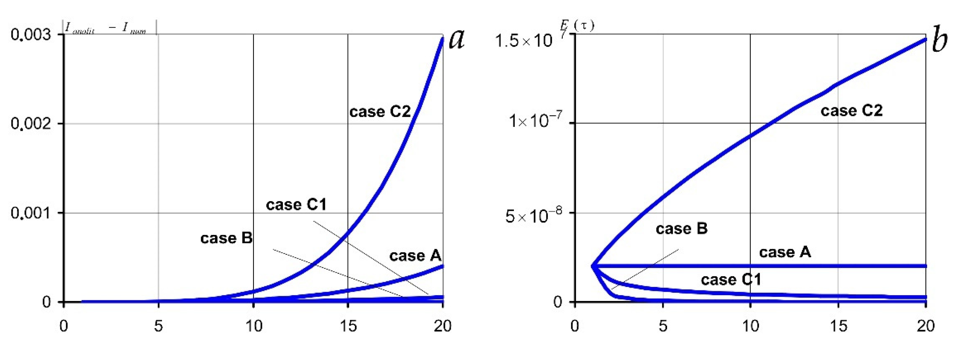
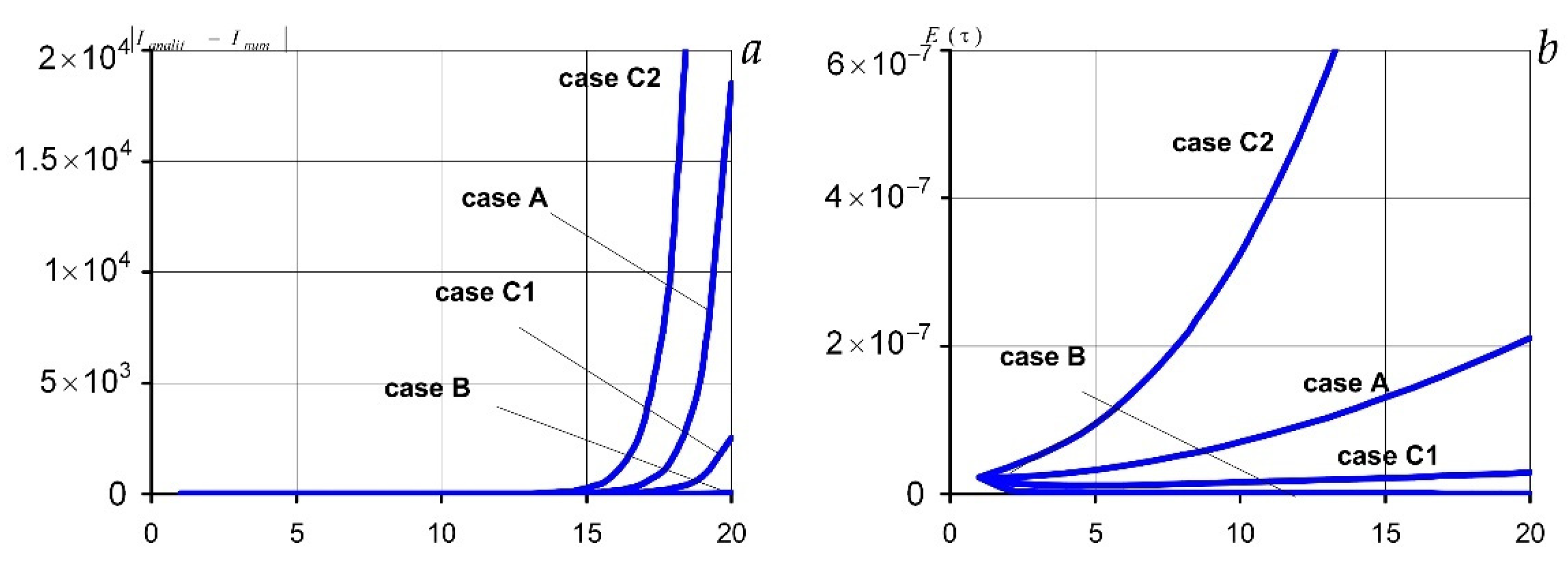
Figure 7 demonstrates comparative graphs of absolute and relative errors in numerical integration by Formula (15) of the case of A, (16) of the case of B, (17) of the cases of C1 for increasing function n(τ) and C2 for decreasing n(τ).

Note that the values closest to the analytical values of the integral are obtained in the case of the constant width of the grid and of increase in the number of partition elements together with an increase in the integration (Figure 7a,b). The results calculated by the Formula (17) at the imposition of the increasing function of nodes quantity n(τ) (case C1, Figure 7) show that the values of absolute and relative errors are quite acceptable. However, in this case, the number of operations is smaller than in the case of B. Note that only one case C2, i.e., imposition of the decreasing function of the number of nodes n(τ), leads to a sharp increase in absolute and relative errors with increasing τ and can go beyond a given accuracy of calculations (Figure 7, Table 4). In the cases of A, B, and C1 the difference between the analytical and numerical calculations of |I_analyt − I_num| is within the acceptable deviation.

In this case, at a denser grid overlaid on the variable region of integration both absolute and relative errors decrease. In particular, the difference |I_analyt − I_num| decreases by two orders of magnitude when n increases by an order (Table 1, Table 2, Table 3 and Table 4).

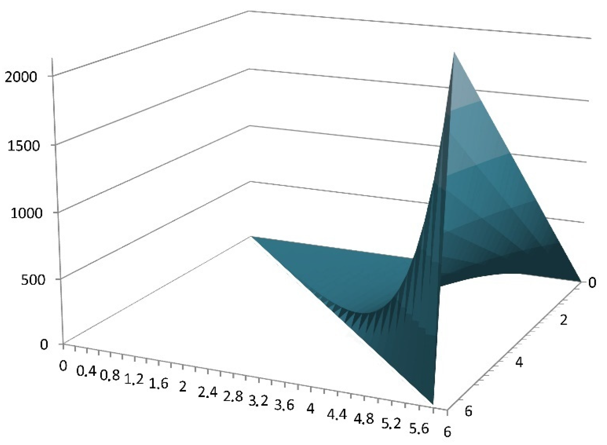
II. Consider next integrand f(τ′, τ″) = e^τ′τ″ for the same values of τ. The surface formed by the function f(τ′, τ″) over the integration region is shown in Figure 8.

We also calculate the integral $I_{num}=$ ${\displaystyle \underset{0}{\overset{\mathsf{\tau }}{\int }}{\displaystyle \underset{0}{\overset{{\mathsf{\tau }}^{\prime }}{\int }}{e}^{{\mathsf{\tau }}^{\prime }}{\mathsf{\tau }}^{″}d{\mathsf{\tau }}^{\prime }d{\mathsf{\tau }}^{″}}}$ by Formulas (15)–(17). The analytical expression has been found in the form $I_{analyt}=$ $\frac{1}{2}{e}^{\mathsf{\tau }}\left({\mathsf{\tau }}^2-2\mathsf{\tau }+2\right)-1$.

The results of calculations are presented in

Table 5. Calculation of integral ${\displaystyle \underset{0}{\overset{\mathsf{\tau }}{\int }}{\displaystyle \underset{0}{\overset{{\mathsf{\tau }}^{\prime }}{\int }}\exp ({\mathsf{\tau }}^{\prime }){\mathsf{\tau }}^{″}d{\mathsf{\tau }}^{\prime }d{\mathsf{\tau }}^{″}}}$ for the case of A.

n(τ)	h(τ)	τ	${\mathit{V}}_{\mathit{s}{\mathit{q}}_{\mathit{e}\mathit{l}}}$	${\mathit{V}}_{\mathit{t}{\mathit{r}}_{\mathit{e}\mathit{l}}}$	Ianalyt	Inum	|Ianalyt − Inum|	E(τ)
104	0.0001	1	0.359090906	0.00005	0.359140914	0.359140906	0.000000008	2.267 × 10−8
104	0.0002	2	6.388217048	0.000838906	6.389056099	6.389055954	0.000000145	2.271 × 10−8
104	0.0003	3	49.207665438	0.006175661	49.213842308	49.213841099	0.000001209	2.457 × 10−8
104	0.0004	4	271.957783692	0.032958890	271.990750166	271.990742582	0.000007584	2.788 × 10−8
104	0.0005	5	1260.363148341	0.148663157	1260.511852372	1260.511811497	0.000040874	3.243 × 10−8
104	0.0006	6	5242.968672666	0.605443177	5243.574315406	5243.574115843	0.000199562	3.806 × 10−8
104	0.0007	7	2.028440925 × 104	2.303279570	2.0286713430927 × 104	2.028671252433 × 104	0.000906595	4.469 × 10−8
104	0.0008	8	74514.5987 × 104	8.347082077	7.4522.949676043 × 104	7.452294578116 × 104	0.003894878	5.226 × 10−8
104	0.0009	9	2.633200401 × 105	29.171550908	2.633492276462 × 105	2.633492116479 × 105	0.015998222	6.075 × 10−8
104	0.001	10	9.029849147 × 105	99.119591029	9.0308409758708 × 105	9.030840342614 × 105	0.063325711	7.012 × 10−8
104	0.0011	11	3.023313605 × 106	329.30830951	3.0236431566175 × 106	3.023642913616 × 106	0.243001233	8.037 × 10−8
104	0.0012	12	9.926966186 × 106	1074.1821472	9.9280412765592 × 106	9.928040368388 × 106	0.908171151	9.148 × 10−8
104	0.0013	13	3.207151578 × 107	3450.8248242	3.2074969920647 × 107	3.207496660282 × 107	3.317823097	1.034 × 10−7
104	0.0014	14	1.022104076 × 108	1.09436987 × 104	1.0222136315401 × 108	1.022213512703 × 108	11.883732932	1.163 × 10−7
104	0.0015	15	3.219638437 × 108	3.43246795 × 104	3.219982101885 × 108	3.219981683553 × 108	41.833202855	1.299 × 10−7
104	0.0016	16	1.004023709 × 109	1.06633314 × 105	1.0041304878174 × 109	1.004130342796 × 109	145.021310075	1.444 × 10−7
104	0.0017	17	3.103582425 × 109	3.28507313 × 105	3.1039114278344 × 109	3.103910931908 × 109	495.926285982	1.598 × 10−7
104	0.0018	18	9.519689251 × 109	1.00459738 × 106	9.5206955239129 × 109	9.520693848599 × 109	1675.31390521	1.760 × 10−7
104	0.0019	19	2.900031626 × 1010	3.05204684 × 106	2.9003373905518 × 1010	2.9003368308 × 1010	5597.53888766	1.930 × 10−7
104	0.002	20	8.780566371 × 1010	9.21813702 × 106	8.781490036817 × 1010	8.7814881851 × 1010	1.85171357 × 104	2.109 × 10−7

,

Table 6. Calculation of integral ${\displaystyle \underset{0}{\overset{\mathsf{\tau }}{\int }}{\displaystyle \underset{0}{\overset{{\mathsf{\tau }}^{\prime }}{\int }}\exp ({\mathsf{\tau }}^{\prime }){\mathsf{\tau }}^{″}d{\mathsf{\tau }}^{\prime }d{\mathsf{\tau }}^{″}}}$ for the case of B.

n(τ)	h(τ)	τ	${\mathit{V}}_{\mathit{s}{\mathit{q}}_{\mathit{e}\mathit{l}}}$	${\mathit{V}}_{\mathit{t}{\mathit{r}}_{\mathit{e}\mathit{l}}}$	Ianalyt	Inum	|Ianalyt − Inum|	E(τ)
1 × 104	0.0001	1	0.359090906	0.000050000	0.359140914	0.359140906	0.000000008	2.267 × 10−8
2 × 104	0.0001	2	6.38863661	0.000419453	6.389056099	6.389056063	0.000000036	5.682 × 10−9
3 × 104	0.0001	3	49.21178362	0.002058554	49.213842308	49.21384217	0.000000134	2.723 × 10−9
4 × 104	0.0001	4	271.98251	0.008239722	271.990750166	271.9907497	0.000000474	1.743 × 10−9
5 × 104	0.0001	5	1260.482118	0.029732632	1260.511852372	1260.511851	0.00000163	1.293 × 10−9
6 × 104	0.0001	6	5243.473403	0.100907198	5243.574315406	5243.57431	0.00000554	1.057 × 10−9
7 × 104	0.0001	7	2.028638 × 104	0.329039947	2.0286713431 × 104	2.028671341 × 104	0.0000185	9.119 × 10−10
8 × 104	0.0001	8	7.452191 × 104	1.043385295	7.4522.949676 × 104	7.452294962 × 104	0.0000609	8.172 × 10−10
9 × 104	0.0001	9	2.633168 × 105	32.41283402	2.63349.227646 × 105	2.633492274 × 105	0.000197509	7.5 × 10−10
10 × 104	0.0001	10	9.02985 × 105	99.11959103	9.03084097587 × 105	9.03084.097 × 105	0.000633257	7.012 × 10−10
11 × 104	0.0001	11	3.023344 × 106	299.3711936	3.023643.15661 × 106	3.023643155 × 106	0.002008275	6.642 × 10−10
12 × 104	0.0001	12	9.927146 × 106	895.1518087	9.928041.27656 × 106	9.92804127 × 106	0.006306744	6.352 × 10−10
13 × 104	0.0001	13	3.207232 × 107	2654.480723	3.20749699206 × 107	3.2074969 × 107	0.01963209	6.121 × 10−10
14 × 104	0.0001	14	1.0221355 × 108	7816.927971	1.02221363154 × 108	1.02221363 × 108	0.060631293	5.931 × 10−10
15 × 104	0.0001	15	3.21975326 × 108	2.2883121 × 104	3.21998210189 × 108	3.2199821 × 108	0.185925351	5.774 × 10−10
16 × 104	0.0001	16	1.00406384 × 109	6.6645826 × 104	1.00413048782 × 109	1.004130487 × 109	0.566489518	5.642 × 10−10
17 × 104	0.0001	17	3.10371819 × 109	1.9323961 × 105	3.10391142783 × 109	3.103911426 × 109	1.716008036	5.529 × 10−10
18 × 104	0.0001	18	9.52013741 × 109	5.5810971 × 105	9.52069552391 × 109	9.520695519 × 109	5.170722441	5.431 × 10−10
19 × 104	0.0001	19	2.9001768 × 1010	1.6063406 × 106	2.9003373906 × 1010	2.900337389 × 1010	15.50564977	5.346 × 10−10
20 × 104	0.0001	20	8.7810291 × 1010	4.6090691 × 106	8.7814900368 × 1010	8.781490032 × 1010	46.29284612	5.272 × 10−10

,

Table 7. Calculation of integral ${\displaystyle \underset{0}{\overset{\mathsf{\tau }}{\int }}{\displaystyle \underset{0}{\overset{{\mathsf{\tau }}^{\prime }}{\int }}\exp ({\mathsf{\tau }}^{\prime }){\mathsf{\tau }}^{″}d{\mathsf{\tau }}^{\prime }d{\mathsf{\tau }}^{″}}}$ for the case of C for increasing function $n(\mathsf{\tau })={10}^4·\sqrt[3]{\mathsf{\tau }}$.

n(τ)	h(τ)	τ	${\mathit{V}}_{\mathit{s}{\mathit{q}}_{\mathit{e}\mathit{l}}}$	${\mathit{V}}_{\mathit{t}{\mathit{r}}_{\mathit{e}\mathit{l}}}$	Ianalyt	Inum	|Ianalyt − Inum|	E(τ)
1 × 104	0.0001	1	0.359090906	0.00005	0.359140914	0.359140906	0.000000008	2.267 × 10−8
1.2599 × 104	0.000159	2	6.388390157	0.000665851	6.389056099	6.389056008	0.000000091	1.431 × 10−8
1.4422 × 104	0.000208	3	49.209559615	0.004282111	49.21384231	49.213841727	0.000000581	1.181 × 10−8
1.5874 × 104	0.000252	4	271.969984343	0.020762813	271.9907502	271.990747156	0.000003010	1.107 × 10−8
1.71 × 104	0.000292	5	1260.424900874	0.086937519	1260.511852	1260.511838393	0.000013978	1.109 × 10−8
1.8171 × 104	0.000330	6	5243.241062964	0.333192002	5243.574315	5243.574254966	0.000060439	1.153 × 10−8
1.9129 × 104	0.000366	7	2.028550910579 × 104	1.204077378	2.028671343 × 104	2.0286713183168 × 104	0.000247759	1.221 × 10−8
2 × 104	0.000400	8	7.451877516118 × 104	4.173541146	7.452294968 × 104	7.4522948702324 × 104	0.000973719	1.307 × 10−8
2.0801 × 104	0.000433	9	2.633351998384 × 105	14.02411031	2.633492276 × 105	2.63349223948742 × 105	0.003697458	1.404 × 10−8
2.1544 × 104	0.000464	10	9.030380759622 × 105	46.007981335	9.030840976 × 105	9.03084083943526 × 105	0.013643550	1.511 × 10−8
2.224 × 104	0.000495	11	3.023495037198 × 106	148.0702902	3.023643157 × 106	3.02364310748837 × 106	0.049129116	1.625 × 10−8
2.2894 × 104	0.000524	12	9.927571905155 × 106	469.198134373	9.928041277 × 106	9.92804110328883 × 106	0.173270407	1.745 × 10−8
2.3513 × 104	0.000553	13	3.207350169621 × 107	1467.6243169	3.207496992 × 107	3.20749693205281 × 107	0.600118610	1.871 × 10−8
2.4101 × 104	0.000581	14	1.022168203424 × 108	4540.7657393	1.022213632 × 108	1.02221361108113 × 108	2.045892619	2.001 × 10−8
2.4662 × 104	0.000608	15	3.219842852655 × 108	1.391804499 × 104	3.219982102 × 108	3.21998203310464 × 108	6.878038824	2.136 × 10−8
2.5198 × 104	0.000635	16	1.004088146807 × 109	4.23181701 × 104	1.004130488 × 109	1.0041304649772 × 109	22.840187703	2.275 × 10−8
2.5713 × 104	0.000661	17	3.103783593579 × 109	1.277592469 × 105	3.103911428 × 109	3.10391135282573 × 109	75.008696351	2.417 × 10−8
2.6207 × 104	0.000687	18	9.520311948239 × 109	3.83331.746 × 105	9.520695524 × 109	9.52069527998495 × 109	243.927973829	2.562 × 10−8
2.6684 × 104	0.000712	19	2.90022293451 × 1010	1.143774275 × 106	2.900337391 × 1010	2.90033731193863 × 1010	786.131675605	2.71 × 10−8
2.7144 × 104	0.000737	20	8.78115018417 × 1010	3.396013293 × 106	8.781490037 × 1010	8.78148978549772 × 1010	2513.194845602	2.862 × 10−8

and

Table 8. Calculation of integral ${\displaystyle \underset{0}{\overset{\mathsf{\tau }}{\int }}{\displaystyle \underset{0}{\overset{{\mathsf{\tau }}^{\prime }}{\int }}\exp ({\mathsf{\tau }}^{\prime }){\mathsf{\tau }}^{″}d{\mathsf{\tau }}^{\prime }d{\mathsf{\tau }}^{″}}}$ for the case of C for decreasing function $n(\mathsf{\tau })={10}^4/\sqrt[3]{\mathsf{\tau }}$.

n(τ)	h(τ)	τ	${\mathit{V}}_{\mathit{s}{\mathit{q}}_{\mathit{e}\mathit{l}}}$	${\mathit{V}}_{\mathit{t}{\mathit{r}}_{\mathit{e}\mathit{l}}}$	Ianalyt	Inum	|Ianalyt − Inum|	E(τ)
1 × 104	0.0001	1	0.359090906	0.00005	0.359140914	0.359140906	0.000000008	2.267 × 10−8
7937	0.00025	2	6.387998913	0.001056956	6.389056099	6.389055869	0.00000023	3.605 × 10−8
6934	0.00043	3	49.204933446	0.008906347	49.21384231	49.213839793	0.000002515	5.11 × 10−8
6300	0.00063	4	271.938415361	0.052315697	271.9907502	271.990731058	0.000019107	7.025× 10−8
5848	0.00085	5	1260.257520896	0.254211957	1260.511852	1260.511732853	0.000119519	9.482 × 10−8
5503	0.00109	6	5242.473450803	1.100205612	5243.574315	5243.573656415	0.00065899	1.257 × 10−7
5228	0.00134	7	2.028230445327 × 104	4.405660679	2.028671343 × 104	2.0286710113953 × 104	0.003316973	1.635 × 10−7
5000	0.00160	8	7.45062399341 × 104	16.694162437	7.452294968 × 104	7.4522934096532 × 104	0.015579511	2.091 × 10−7
4807	0.00187	9	2.6328847285547 × 105	60.685556091	2.633492276 × 105	2.63349158411563 × 105	0.069234637	2.629 × 10−7
4642	0.00215	10	9.0287027597645 × 105	213.527730828	9.030840976 × 105	9.03083803707273 × 105	0.293879802	3.254 × 10−7
4496	0.00245	11	3.0229095073427 × 106	732.447132721	3.023643157 × 106	3.02364195447544 × 106	1.202142053	3.976 × 10−7
4368	0.00275	12	9.925577309137 × 106	2459.207472851	9.928041277 × 106	9.92803651660984 × 106	4.759949403	4.794 × 10−7
4253	0.00306	13	3.206683772061 × 107	8113.8573721	3.207496992 × 107	3.2074951.5779861 × 107	18.3426607	5.719 × 10−7
4149	0.00337	14	1.0219491741747 × 108	26376.7020856 × 104	1.022213632 × 108	1.02221294119557 × 108	69.0344492	6.753 × 10−7
4055	0.00370	15	3.2191330803007 × 108	8.4647745487 × 104	3.219982102 × 108	3.21997955775555 × 108	254.4129479	7.901 × 10−7
3969	0.00403	16	1.0038609019518 × 109	2.68665268872 × 105	1.004130488 × 109	1.00412956722071 × 109	920.5966830	9.168 × 10−7
3889	0.00437	17	3.1030634405218 × 109	8.44708315902 × 105	3.103911428 × 109	3.10390814883765 × 109	3278.9967729	1.056 × 10−6
3816	0.00472	18	9.5180514287336 × 109	2.63259037681 × 106	9.520695524 × 109	9.52068401911039 × 109	1.1504802533 × 104	1.208 × 10−6
3748	0.00507	19	2.8995190932092 × 1010	8.14312624403 × 106	2.900337391 × 1010	2.90033340583357 × 1010	3.9847182199 × 104	1.374 × 10−6
3684	0.00543	20	8.7789741872444 × 1010	2.50220580946 × 107	8.781490037 × 1010	8.78147639305388 × 1010	1.3643763326 × 105	1.554 × 10−6

for different numbers of triangular elements n(τ) and grid width h(τ).

Table 5 shows the corresponding values for the case when only the size of the imposed grid h(τ) changes with the change of τ, (A). The calculated values for the case when only the number of division elements $N_{el}(\mathsf{\tau })$ changes with the change of τ, (B) are presented in Table 6. In Table 7 and Table 8 it is shown the values of integration parameters for the case when with the change of τ, both the size of the grid and the number of division elements change (C), namely for $n(\mathsf{\tau })={10}^4·\sqrt[3]{\mathsf{\tau }}$, $h(t)={10}^{-4}·\sqrt[3]{{\mathsf{\tau }}^2}$ and $n(\mathsf{\tau })={10}^4/\sqrt[3]{\mathsf{\tau }}$, $h(t)={10}^{-4}·\sqrt[3]{{\mathsf{\tau }}^4}$ correspondingly.

Figure 9 demonstrates comparative graphs of absolute (Figure 9a) and relative (Figure 9b) errors in numerical integration ${\displaystyle \underset{0}{\overset{\mathsf{\tau }}{\int }}{\displaystyle \underset{0}{\overset{{\mathsf{\tau }}^{\prime }}{\int }}\exp ({\mathsf{\tau }}^{\prime }){\mathsf{\tau }}^{″}d{\mathsf{\tau }}^{\prime }d{\mathsf{\tau }}^{″}}}$ by Formula (15) of the case of A, (16) of the case of B, (17) of the cases of C1 for increasing function n(τ) and C2 for decreasing n(τ).

When the integrand contains an exponential function, the sharp increase in the integrand has almost no effect on the value of both absolute and relative errors for numerical calculation of the integral by Formulas (16) and (17) under the increasing function of the number of nodes, i.e., case C1 (Figure 9, Table 6 and Table 7).

For this integral, the difference between the analytical and numerical calculation |I_analyt − I_num| is also within the acceptable deviation for the cases of A, B, and C1. However, as distinct from the previous case I, the magnitude of this difference is an order larger. So, for the case of B and $n(\mathsf{\tau })={10}^4$, $\mathsf{\tau }=20$ ${E(\mathsf{\tau })|}_{f({\mathsf{\tau }}^{\prime },{\mathsf{\tau }}^{″})={\mathsf{\tau }}^{\prime }{\mathsf{\tau }}^{″},}~{10}^{-11}$, but ${E(\mathsf{\tau })|}_{f({\mathsf{\tau }}^{\prime },{\mathsf{\tau }}^{″})=e^{{\mathsf{\tau }}^{\prime }}{\mathsf{\tau }}^{″}}~{10}^{-10}$ (Table 2 and Table 6). Herewith, when increasing n by an order of magnitude, the relative error decreases by two orders.

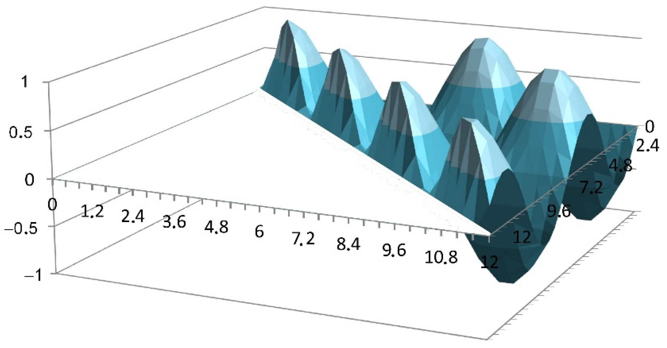
III. Now we consider the integrand f(τ′, τ″) = sin(τ′)sin(τ″) for the same values of τ. The surface formed by the function f(τ′, τ″) over the integration region is shown in Figure 10.

The integral $I_{num}=$ ${\displaystyle \underset{0}{\overset{\mathsf{\tau }}{\int }}{\displaystyle \underset{0}{\overset{{\mathsf{\tau }}^{\prime }}{\int }}{e}^{{\mathsf{\tau }}^{\prime }}{\mathsf{\tau }}^{″}d{\mathsf{\tau }}^{\prime }d{\mathsf{\tau }}^{″}}}$ is also calculated by Formulas (15)–(17). The analytical expression has been found in the form $I_{analyt}=$ $\frac{1}{4}\sin (2\mathsf{\tau })+\frac{1}{2}\mathsf{\tau }$.

The results of calculations are presented in

Table 9. Calculation of integral ${\displaystyle \underset{0}{\overset{\mathsf{\tau }}{\int }}{\displaystyle \underset{0}{\overset{{\mathsf{\tau }}^{\prime }}{\int }}\sin ({\mathsf{\tau }}^{\prime })\sin ({\mathsf{\tau }}^{″})d{\mathsf{\tau }}^{\prime }d{\mathsf{\tau }}^{″}}}$ for the case of A.

n(τ)	h(τ)	τ	${\mathit{V}}_{\mathit{s}{\mathit{q}}_{\mathit{e}\mathit{l}}}$	${\mathit{V}}_{\mathit{t}{\mathit{r}}_{\mathit{e}\mathit{l}}}$	Ianalyt	Inum	|Ianalyt − Inum|	E(τ)
104	0.0001	1	0.105647349	1.36 × 10−5	0.105660985	0.105660983	2.2104 × 10−9	2.092 × 10−8
104	0.0002	2	1.002616986	0.00011892	1.002735931	1.002735906	2.498 × 10−8	2.4912 × 10−8
104	0.0003	3	1.979799515	0.000235478	1.980035068	1.980034994	7.4699 × 10−8	3.7726 × 10−8
104	0.0004	4	1.366917966	0.000350532	1.367268612	1.367268498	1.1406 × 10−7	8.3423 × 10−8
104	0.0005	5	0.255910847	0.000659001	0.256569932	0.256569848	8.4197 × 10−8	3.2816 × 10−7
104	0.0006	6	−0.000147047	0.000940243	0.000793203	0.000793196	7.1455 × 10−9	9.0085 × 10−6
104	0.0007	7	0.029143669	0.001138322	0.03028205	0.030281991	5.9057 × 10−8	1.9502 × 10−6
104	0.0008	8	0.654456042	0.00162879	0.656085164	0.656084832	3.3157 × 10−7	5.0537 × 10−7
104	0.0009	9	1.824099302	0.002109486	1.826209439	1.826208788	6.5074 × 10−7	3.5633 × 10−7
104	0.001	10	1.688705384	0.002385882	1.691092045	1.691091266	7.7861 × 10−7	4.6042 × 10−7
104	0.0011	11	0.492557326	0.003026217	0.495584095	0.495583543	5.5235 × 10−7	1.1145 × 10−6
104	0.0012	12	0.008454845	0.003735837	0.012190793	0.012190682	1.1096 × 10−7	9.1021 × 10−6
104	0.0013	13	0.000181887	0.004101084	0.004283049	0.004282972	7.7604 × 10−8	1.8119 × 10−5
104	0.0014	14	0.367757939	0.004852591	0.372611315	0.37261053	7.8514 × 10−7	2.1071 × 10−6
104	0.0015	15	1.54243883	0.005810256	1.548250775	1.548249086	1.6894 × 10−6	1.0911 × 10−6
104	0.0016	16	1.909923509	0.006289715	1.91621532	1.916213223	2.097 × 10−6	1.0944 × 10−6
104	0.0017	17	0.805906553	0.00711257	0.813020769	0.813019123	1.6468 × 10−6	2.0255 × 10−6
104	0.0018	18	0.049368684	0.00832315	0.057692369	0.057691835	5.3471 × 10−7	9.2683 × 10−6
104	0.0019	19	−0.00889084	0.008954612	6.38 × 10−5	6.38 × 10−5	2.0367 × 10−8	3.1927 × 10−4
104	0.002	20	0.165368576	0.009813722	0.175183423	0.175182297	1.1254 × 10−6	6.4243 × 10−6

,

Table 10. Calculation of integral ${\displaystyle \underset{0}{\overset{\mathsf{\tau }}{\int }}{\displaystyle \underset{0}{\overset{{\mathsf{\tau }}^{\prime }}{\int }}\sin ({\mathsf{\tau }}^{\prime })\sin ({\mathsf{\tau }}^{″})d{\mathsf{\tau }}^{\prime }d{\mathsf{\tau }}^{″}}}$ for the case B.

n(τ)	h(τ)	τ	${\mathit{V}}_{\mathit{s}{\mathit{q}}_{\mathit{e}\mathit{l}}}$	${\mathit{V}}_{\mathit{t}{\mathit{r}}_{\mathit{e}\mathit{l}}}$	Ianalyt	Inum	|Ianalyt − Inum|	E(τ)
1 × 104	0.0001	1	0.105524426	0.000136557	0.105660985	0.105660983	2.2104 × 10−9	2.092 × 10−8
2 × 104	0.0001	2	1.002140706	0.000595219	1.002735931	1.002735925	6.2451 × 10−9	6.2281 × 10−9
3 × 104	0.0001	3	1.979249311	0.000785749	1.980035068	1.98003506	8.2999 × 10−9	4.1918 × 10−9
4 × 104	0.0001	4	1.366391569	0.000877036	1.367268612	1.367268605	7.1288 × 10−9	5.2139 × 10−9
5 × 104	0.0001	5	0.255251593	0.001318336	0.256569932	0.256569929	3.3679 × 10−9	1.3127 × 10−8
6 × 104	0.0001	6	−0.000773888	0.001567091	0.000793203	0.000793203	1.9849 × 10−10	2.5023 × 10−7
7 × 104	0.0001	7	0.028655756	0.001626293	0.03028205	0.030282049	1.2053 × 10−9	3.9801 × 10−8
8 × 104	0.0001	8	0.654048658	0.002036501	0.656085164	0.656085159	5.1808 × 10−9	7.8965 × 10−9
9 × 104	0.0001	9	1.823864762	0.002344669	1.826209439	1.826209431	8.0338 × 10−9	4.3992 × 10−9
10 × 104	0.0001	10	1.688705384	0.002386653	1.691092045	1.691092037	7.7861 × 10−9	4.6042 × 10−9
11 × 104	0.0001	11	0.492832533	0.002751558	0.495584095	0.495584091	4.5649 × 10−9	9.2111 × 10−9
12 × 104	0.0001	12	0.009077519	0.003113274	0.012190793	0.012190792	7.7057 × 10−10	6.3209 × 10−8
13 × 104	0.0001	13	0.001128323	0.003154726	0.004283049	0.004283049	4.592 × 10−10	1.0721 × 10−7
14 × 104	0.0001	14	0.369144778	0.003466533	0.372611315	0.372611311	4.0058 × 10−9	1.0751 × 10−8
15 × 104	0.0001	15	1.544376521	0.003874247	1.548250775	1.548250768	7.5082 × 10−9	4.8495 × 10−9
16 × 104	0.0001	16	1.91228343	0.003931883	1.91621532	1.916215312	8.1915 × 10−9	4.2748 × 10−9
17 × 104	0.0001	17	0.808836335	0.004184429	0.813020769	0.813020764	5.6983 × 10−9	7.0088 × 10−9
18 × 104	0.0001	18	0.053068232	0.004624136	0.057692369	0.057692368	1.6503 × 10−9	2.8606 × 10−8
19 × 104	0.0001	19	−0.004649167	0.00471296	6.37928 × 10−5	6.37928 × 10−5	5.6423 × 10−11	8.8446 × 10−7
20 × 104	0.0001	20	0.170276281	0.004907139	0.175183423	0.17518342	2.8136 × 10−9	1.6061 × 10−8

,

Table 11. Calculation of integral ${\displaystyle \underset{0}{\overset{\mathsf{\tau }}{\int }}{\displaystyle \underset{0}{\overset{{\mathsf{\tau }}^{\prime }}{\int }}\sin ({\mathsf{\tau }}^{\prime })\sin ({\mathsf{\tau }}^{″})d{\mathsf{\tau }}^{\prime }d{\mathsf{\tau }}^{″}}}$ for the case of C for increasing function $n(\mathsf{\tau })={10}^4·\sqrt[3]{\mathsf{\tau }}$.

n(τ)	h(τ)	τ	${\mathit{V}}_{\mathit{s}{\mathit{q}}_{\mathit{e}\mathit{l}}}$	${\mathit{V}}_{\mathit{t}{\mathit{r}}_{\mathit{e}\mathit{l}}}$	Ianalyt	Inum	|Ianalyt − Inum|	E(τ)
1 × 104	0.0001	1	0.105647349	1.36 × 10−5	0.105660985	0.105660983	2.2104 × 10−9	2.0920 × 10−8
1.2599 × 104	0.000158743	2	1.002641527	9.44 × 10−5	1.002735931	1.002735916	1.5737 × 10−8	1.5694 × 10−8
1.4422 × 104	0.000208016	3	1.979871755	0.000163277	1.980035068	1.980035032	3.5914 × 10−8	1.8138 × 10−8
1.5874 × 104	0.000251984	4	1.367047746	0.000220822	1.367268612	1.367268567	4.5265 × 10−8	3.3106 × 10−8
1.71 × 104	0.000292398	5	0.256184523	0.000385381	0.256569932	0.256569903	2.8794 × 10−8	1.1223 × 10−7
1.8171 × 104	0.000330196	6	0.000275759	0.000517442	0.000793203	0.000793201	2.1641 × 10−9	2.7283 × 10−6
1.9129 × 104	0.000365937	7	0.029686958	0.000595077	0.03028205	0.030282034	1.6139 × 10−8	5.3297 × 10−7
2 × 104	0.0004	8	0.655270686	0.000814395	0.656085164	0.656085081	8.2892 × 10−8	1.2634 × 10−7
2.0801 × 104	0.000432672	9	1.825195161	0.001014127	1.826209439	1.826209289	1.5040 × 10−7	8.2355 × 10−8
2.1544 × 104	0.000464166	10	1.689984431	0.001107446	1.691092045	1.691091877	1.6775 × 10−7	9.9198 × 10−8
2.224 × 104	0.000494604	11	0.494223275	0.001360709	0.495584095	0.495583984	1.1167 × 10−7	2.2533 × 10−7
2.2894 × 104	0.000524155	12	0.010558975	0.001631797	0.012190793	0.012190772	2.1171 × 10−8	1.7366 × 10−6
2.3513 × 104	0.000552886	13	0.002538858	0.001744177	0.004283049	0.004283035	1.4037 × 10−8	3.2773 × 10−6
2.4101 × 104	0.000580889	14	0.37059774	0.00201344	0.372611315	0.37261118	1.3517 × 10−7	3.6276 × 10−7
2.4662 × 104	0.000608223	15	1.545894543	0.002355955	1.548250775	1.548250498	2.7776 × 10−7	1.7940 × 10−7
2.5198 × 104	0.000634971	16	1.913718874	0.002496117	1.91621532	1.91621499	3.3027 × 10−7	1.7236 × 10−7
2.5713 × 104	0.000661144	17	0.810254383	0.002766138	0.813020769	0.81302052	2.4908 × 10−7	3.0636 × 10−7
2.6207 × 104	0.000686839	18	0.054516365	0.003175926	0.057692369	0.057692291	7.7854 × 10−8	1.3495 × 10−6
2.6684 × 104	0.000712037	19	−0.003292008	0.003355798	6.38 × 10−5	6.38 × 10−5	2.8606 × 10−9	4.4843 × 10−5
2.7144 × 104	0.000736811	20	0.171567841	0.003615429	0.175183423	0.17518327	1.5275 × 10−7	8.7193 × 10−7

and

Table 12. Calculation of integral ${\displaystyle \underset{0}{\overset{\mathsf{\tau }}{\int }}{\displaystyle \underset{0}{\overset{{\mathsf{\tau }}^{\prime }}{\int }}\sin ({\mathsf{\tau }}^{\prime })\sin ({\mathsf{\tau }}^{″})d{\mathsf{\tau }}^{\prime }d{\mathsf{\tau }}^{″}}}$ for the case of C for decreasing function $n(\mathsf{\tau })={10}^4/\sqrt[3]{\mathsf{\tau }}$.

n(τ)	h(τ)	τ	${\mathit{V}}_{\mathit{s}{\mathit{q}}_{\mathit{e}\mathit{l}}}$	${\mathit{V}}_{\mathit{t}{\mathit{r}}_{\mathit{e}\mathit{l}}}$	Ianalyt	Inum	|Ianalyt − Inum|	E(τ)
104	0.0001	1	0.105647349	1.36 × 10−5	0.105660985	0.105660983	2.2104 × 10−9	2.092 × 10−8
7937	0.000251984	2	1.002586062	0.00014983	1.002735931	1.002735892	3.9654 × 10−8	3.9546 × 10−8
6934	0.000432651	3	1.979695314	0.000339599	1.980035068	1.980034913	1.5536 × 10−7	7.8465 × 10−8
6300	0.000634921	4	1.366711925	0.0005564	1.367268612	1.367268325	2.8738 × 10−7	2.1019 × 10−7
5848	0.000854993	5	0.255442803	0.001126883	0.256569932	0.256569686	2.462 × 10−7	9.5957 × 10−7
5503	0.001090314	6	−0.000915421	0.001708601	0.000793203	0.000793179	2.3596 × 10−8	2.9747 × 10−5
5228	0.001338944	7	0.028104478	0.002177356	0.03028205	0.030281834	2.1607 × 10−7	7.1354 × 10−6
5000	0.0016	8	0.652826257	0.003257581	0.656085164	0.656083837	1.3263 × 10−6	2.0215 × 10−6
4807	0.00187227	9	1.82181826	0.004388363	1.826209439	1.826206623	2.8162 × 10−6	1.5421 × 10−6
4642	0.002154244	10	1.68594866	0.005139771	1.691092045	1.691088431	3.6134 × 10−6	2.1367 × 10−6
4496	0.002446619	11	0.488850453	0.00673091	0.495584095	0.495581363	2.7325 × 10−6	5.5137 × 10−6
4368	0.002747253	12	0.003637471	0.00855274	0.012190793	0.012190212	5.8157 × 10−7	4.7706 × 10−5
4253	0.003056666	13	−0.005360183	0.009642803	0.004283049	0.00428262	4.2903 × 10−7	1.0017 × 10−4
4149	0.003374307	14	0.360910945	0.01169581	0.372611315	0.372606754	4.561 × 10−6	1.2241 × 10−5
4055	0.003699137	15	1.533911879	0.014328622	1.548250775	1.548240501	1.0274 × 10−5	6.6358 × 10−6
3969	0.004031242	16	1.900354908	0.015847101	1.91621532	1.916202009	1.3312 × 10−5	6.9469 × 10−6
3889	0.004371304	17	0.794720939	0.018288942	0.813020769	0.813009881	1.0888 × 10−5	1.3393 × 10−5
3816	0.004716981	18	0.035877505	0.021811192	0.057692369	0.057688697	3.6719 × 10−6	6.3647 × 10−5
3748	0.00506937	19	−0.02382806	0.023891708	6.38 × 10−5	6.36 × 10−5	1.4492 × 10−7	2.2717 × 10−3
3684	0.005428882	20	0.148536366	0.026638764	0.175183423	0.17517513	8.2924 × 10−6	4.7335 × 10−5

for different numbers of triangular elements n(τ) and grid width h(τ).

Table 9 shows the corresponding values for the case when only the size of the imposed grid h(τ) changes with the change of τ, (A). The calculated values for the case when only the number of division elements $N_{el}(\mathsf{\tau })$ changes with the change of τ, (B) are presented in Table 10. In Table 11 and Table 12 it is shown the values of integration parameters for the case when with the change of τ, both the size of the grid and the number of division elements change (C), namely for $n(\mathsf{\tau })={10}^4·\sqrt[3]{\mathsf{\tau }}$, $h(t)={10}^{-4}·\sqrt[3]{{\mathsf{\tau }}^2}$ and $n(\mathsf{\tau })={10}^4/\sqrt[3]{\mathsf{\tau }}$, $h(t)={10}^{-4}·\sqrt[3]{{\mathsf{\tau }}^4}$ correspondingly.

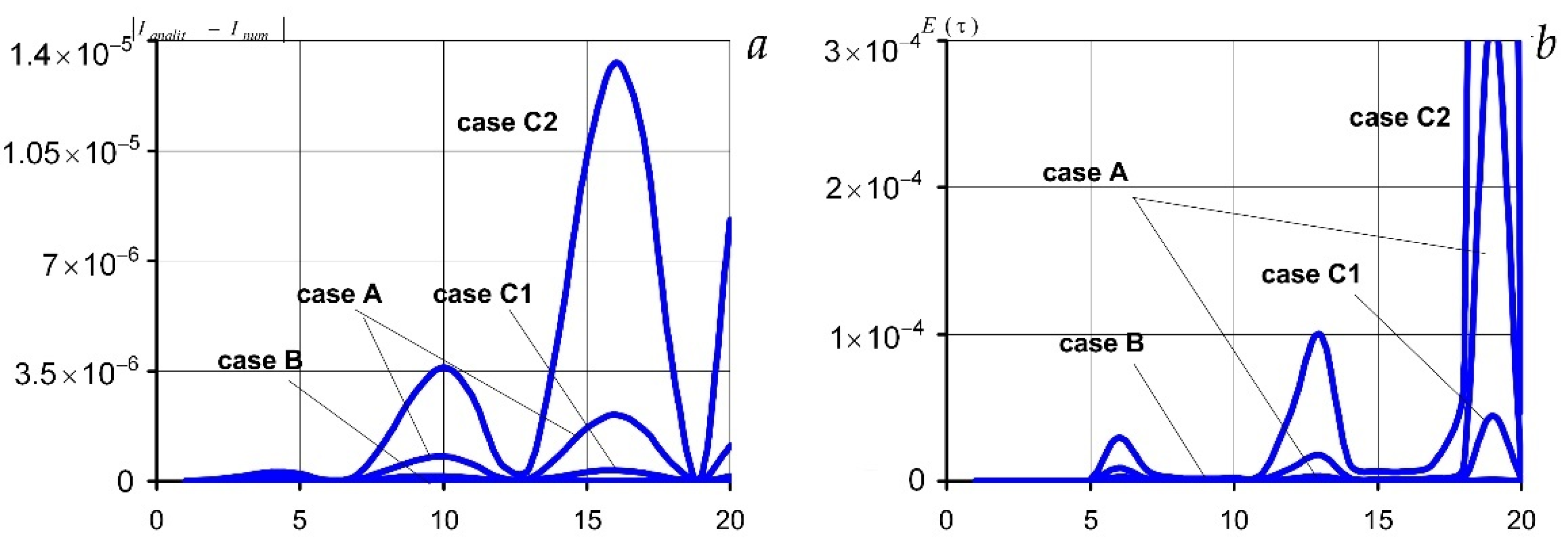
Figure 11 demonstrates comparative graphs of absolute (Figure 11a) and relative (Figure 11b) errors in numerical integration ${\displaystyle \underset{0}{\overset{\mathsf{\tau }}{\int }}{\displaystyle \underset{0}{\overset{{\mathsf{\tau }}^{\prime }}{\int }}\sin ({\mathsf{\tau }}^{\prime })\sin ({\mathsf{\tau }}^{″})d{\mathsf{\tau }}^{\prime }d{\mathsf{\tau }}^{″}}}$ by Formula (15) of the case of A, (16) of the case of B, (17) of the cases of C1 for increasing function n(τ) and C2 for decreasing n(τ).

Note that for the periodic integrand, the closest to the analytical value of the integral is obtained in the case of the constant width of the grid and in the case of an increase in the number of partition elements together with an increase in the integration region (Figure 11a,b). Here the results for the absolute and relative error calculated by the Formula (17) for the imposition of the increasing function of the number of nodes n(τ), case C1 (Figure 11) are quite acceptable. For this integrand, the integration results obtained by Formulas (15)–(17) with increasing τ remain within the given accuracy of calculations (Figure 11, Table 9, Table 10, Table 11 and Table 12).

In this case, the difference between the analytical and numerical calculation |I_analit − I_num| is of the same order as for the integrand $f({\mathsf{\tau }}^{\prime },{\mathsf{\tau }}^{″})={\mathsf{\tau }}^{\prime }{\mathsf{\tau }}^{″}$. When increasing n by an order of magnitude, the value of E(τ) also decreases by two orders of magnitude.

Note that for all three considered integrands, no significant accumulation of machine error was observed.

If we apply the proposed method to calculate the double integral with a given external limit of integration, the result is the same (within accuracy) as the value of the same integral, calculated by Maple. For example, according to the calculations in the Maple integral $I_{\mathsf{\tau }=5}={\displaystyle \underset{0}{\overset{5}{\int }}{\displaystyle \underset{0}{\overset{{\mathsf{\tau }}^{\prime }}{\int }}{\mathsf{\tau }}^{\prime }{\mathsf{\tau }}^{″}d{\mathsf{\tau }}^{\prime }d{\mathsf{\tau }}^{″}}}=78.125$, in our case $I_{\mathsf{\tau }=5}=78.124998438$ (the fifth line from the top in Table 1); integral $I_{\mathsf{\tau }=5}={\displaystyle \underset{0}{\overset{\mathsf{\tau }}{\int }}{\displaystyle \underset{0}{\overset{{\mathsf{\tau }}^{\prime }}{\int }}\exp ({\mathsf{\tau }}^{\prime }){\mathsf{\tau }}^{″}d{\mathsf{\tau }}^{\prime }d{\mathsf{\tau }}^{″}}}=1260.511852372$, in our case $I_{\mathsf{\tau }=5}=1260.511811497$ (the fifth line from the top in Table 5); integral $I_{\mathsf{\tau }=5}={\displaystyle \underset{0}{\overset{\mathsf{\tau }}{\int }}{\displaystyle \underset{0}{\overset{{\mathsf{\tau }}^{\prime }}{\int }}\sin ({\mathsf{\tau }}^{\prime })\sin ({\mathsf{\tau }}^{″})d{\mathsf{\tau }}^{\prime }d{\mathsf{\tau }}^{″}}}=0.256569932$, in our case $I_{\mathsf{\tau }=5}=0.256569848$ (the fifth line from the top in Table 9) under $\epsilon ={10}^{-7}$.

The CPU time of the program module was calculated by the algorithm in [41]. It was determined that the times of program execution for calculation of integral $I_{\mathsf{\tau }=5}={\displaystyle \underset{0}{\overset{5}{\int }}{\displaystyle \underset{0}{\overset{{\mathsf{\tau }}^{\prime }}{\int }}{\mathsf{\tau }}^{\prime }{\mathsf{\tau }}^{″}d{\mathsf{\tau }}^{\prime }d{\mathsf{\tau }}^{″}}}$ were from 2.2189994808 s at $n={10}^4$ and to 215.3279999737 s at $n={10}^5$; of integral $I_{\mathsf{\tau }=5}={\displaystyle \underset{0}{\overset{5}{\int }}{\displaystyle \underset{0}{\overset{{\mathsf{\tau }}^{\prime }}{\int }}\exp ({\mathsf{\tau }}^{\prime }){\mathsf{\tau }}^{″}d{\mathsf{\tau }}^{\prime }d{\mathsf{\tau }}^{″}}}$ were from 4.7030001646 s at $n={10}^4$ and to 463.6879999191 s at $n={10}^5$; of integral $I_{\mathsf{\tau }=5}={\displaystyle \underset{0}{\overset{5}{\int }}{\displaystyle \underset{0}{\overset{{\mathsf{\tau }}^{\prime }}{\int }}\sin ({\mathsf{\tau }}^{\prime })\sin ({\mathsf{\tau }}^{″})d{\mathsf{\tau }}^{\prime }d{\mathsf{\tau }}^{″}}}$ were from 6.4680001466 s at $n={10}^4$ and to 635.4220004054 s at $n={10}^5$.

5. Application of the Method to Calculating the Double Integral with Variable Upper Limits Depending on One External Variable

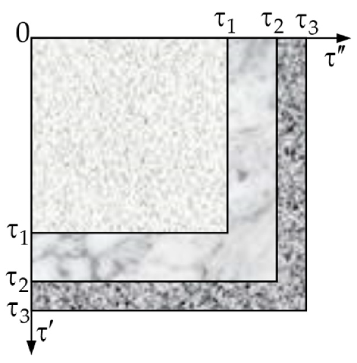
We use the proposed method to calculate double integrals with variable upper limits, which are functions of the external variable τ but do not depend on the integration variables. This kind of integrals is in some sense a partial case of the above integrals with due regard that there is no variable limit ${\mathsf{\tau }}^{″}={\mathsf{\tau }}^{\prime }$ in the region of integration (Figure 3). At the same time, the integration region in ${\displaystyle \underset{0}{\overset{\mathsf{\tau }}{\int }}{\displaystyle \underset{0}{\overset{g(\mathsf{\tau })}{\int }}f({\mathsf{\tau }}^{\prime },{\mathsf{\tau }}^{″},\mathsf{\tau })}d{\mathsf{\tau }}^{″}d{\mathsf{\tau }}^{\prime }}$ is variable.

Taking into account that in all considered examples of the application of the method in chapter 4, the lowest values of absolute and relative errors are achieved in the case of increasing the number of variable elements of division and fixing the grid cell size, i.e., Case B, here we consider only this case of constructing a variable grid.

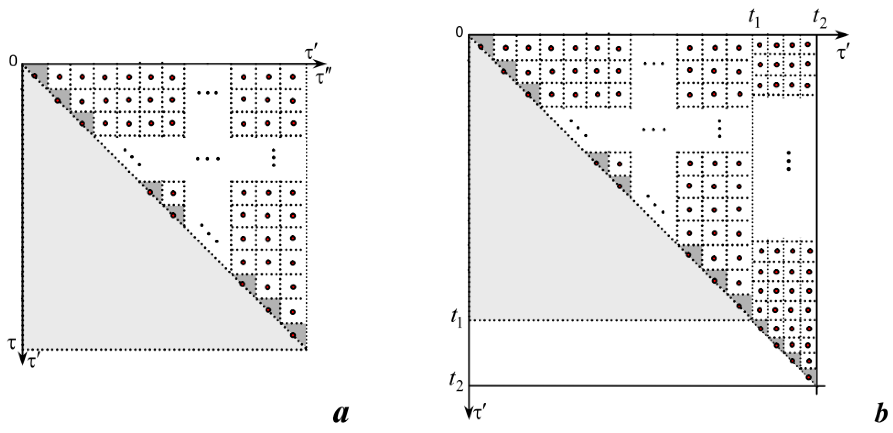
Divide the integration region $[0, g(\mathsf{\tau })]\times [0, \mathsf{\tau }]$ into cells by a rectangular grid that contains $m(\mathsf{\tau })$ elements of the same length $h_m$ along the axis $O{\mathsf{\tau }}^{″}$ and $n(\mathsf{\tau })$ elements of the same length $h_n$ along the axis $O{\mathsf{\tau }}^{\prime }$. Then in the case of B, the cubature formula with weight function $w({\mathsf{\tau }}^{\prime },{\mathsf{\tau }}^{″})\equiv 1$ (16) is modified into the form

$${\displaystyle \underset{0}{\overset{\mathsf{\tau }}{\int }}{\displaystyle \underset{0}{\overset{g(\mathsf{\tau })}{\int }}f({\mathsf{\tau }}^{\prime },{\mathsf{\tau }}^{″},\mathsf{\tau })}d{\mathsf{\tau }}^{″}d{\mathsf{\tau }}^{\prime }}\approx {\displaystyle \sum _{i=1}^{n(\mathsf{\tau })}{\displaystyle \sum _{j=1}^{m(\mathsf{\tau })}{h}_n{h}_m f({{\mathsf{\tau }}^{\prime }}_i,{{\mathsf{\tau }}^{″}}_j,\mathsf{\tau })}},$$

(22)

where ${{\mathsf{\tau }}^{\prime }}_{i+1}={{\mathsf{\tau }}^{\prime }}_i+h_n$; ${{\mathsf{\tau }}^{″}}_{j+1}={{\mathsf{\tau }}^{″}}_j+h_m$.

We obtain the estimation of the error of the method for this case from Formula (21) taking into account the rectangular grid of division of the integration region and the notation introduced here. So, in the general case, we have

$$R(\mathsf{\tau })\approx \frac{h_n(\mathsf{\tau })h_m(\mathsf{\tau })}{24}\left({\displaystyle \underset{\left(V_{{}_{{\mathrm{rectangular}}_{el}}}(\mathsf{\tau })\right)}{\iint }{F^{″}}_{{\mathsf{\tau }}^{\prime }{\mathsf{\tau }}^{\prime }}(\mathsf{\tau },{\mathsf{\tau }}^{\prime },{\mathsf{\tau }}^{″})d{\mathsf{\tau }}^{\prime }d{\mathsf{\tau }}^{″}}+{\displaystyle \underset{\left(V_{{\mathrm{rectangular}}_{el}}(\mathsf{\tau })\right)}{\iint }{F^{″}}_{{\mathsf{\tau }}^{″}{\mathsf{\tau }}^{″}}(\mathsf{\tau },{\mathsf{\tau }}^{\prime },{\mathsf{\tau }}^{″})d{\mathsf{\tau }}^{\prime }d{\mathsf{\tau }}^{″}}\right).$$

or

$$R(\mathsf{\tau })=O(2h_n(\mathsf{\tau })h_m(\mathsf{\tau })).$$

If the lengths of the sides of rectangular cells are constant (fixed), then we obtain the estimation of the method error in the classical form of the error of the cells method [42].

Consider the typical cases of the kind of function g(τ).

(1)

g(τ) = τ.

In this case, the integration region is a square that enlarges equally along both coordinate axes in proportion to the growth τ (Figure 12).

Here we accept $n(\mathsf{\tau })=m(\mathsf{\tau })$, that is we impose a square grid. Then Formula (22) is simplified to the form

$${\displaystyle \underset{0}{\overset{\mathsf{\tau }}{\int }}{\displaystyle \underset{0}{\overset{\mathsf{\tau }}{\int }}f({\mathsf{\tau }}^{\prime },{\mathsf{\tau }}^{″},\mathsf{\tau })}d{\mathsf{\tau }}^{″}d{\mathsf{\tau }}^{\prime }}\approx {\displaystyle \sum _{i=1}^{n(\mathsf{\tau })}{\displaystyle \sum _{j=1}^{n(\mathsf{\tau })}{h}_n^2 f({{\mathsf{\tau }}^{\prime }}_i,{{\mathsf{\tau }}^{″}}_j,\mathsf{\tau })}}.$$

The application of this formula is implemented for the simple integrand $f({\mathsf{\tau }}^{\prime },{\mathsf{\tau }}^{″})={\mathsf{\tau }}^{\prime }{\mathsf{\tau }}^{″}$. The results of the calculations are shown in

Table 13. Calculation of integral ${\displaystyle \underset{0}{\overset{\mathsf{\tau }}{\int }}{\displaystyle \underset{0}{\overset{\mathsf{\tau }}{\int }}{\mathsf{\tau }}^{\prime }{\mathsf{\tau }}^{″}d{\mathsf{\tau }}^{\prime }d{\mathsf{\tau }}^{″}}}$.

n(τ)	h(τ)	τ	Ianalyt	Inum	|Ianalyt − Inum|	E(τ)
104	0.0001	1	0.25	0.2499500000005	4.99999995000368 × 10−5	0.0001999999980001
2 × 104	0.0001	2	4	3.999600000001	0.000399999999001372	9.99999997503431 × 10−5
3 × 104	0.0001	3	20.25	20.2486500000015	0.00134999999849911	6.66666665925489 × 10−5
4 × 104	0.0001	4	64	63.9968000000021	0.00319999999793815	4.99999999677836 × 10−5
5 × 104	0.0001	5	156.25	156.243750000003	0.0062499999974685	3.99999999837984 × 10−5
6 × 104	0.0001	6	324	323.989200000003	0.0107999999970493	3.33333333242263 × 10−5
7 × 104	0.0001	7	600.25	600.232850000004	0.0171499999964412	2.85714285654997 × 10−5
8 × 104	0.0001	8	1024	1023.9744	0.0255999999958128	2.49999999959109 × 10−5
9 × 104	0.0001	9	1640.25	1640.21355	0.0364499999969617	2.22222222203699 × 10−5
105	0.0001	10	2500	2499.95000000001	0.0499999999899683	1.99999999959873 × 10−5
1.1 × 105	0.0001	11	3660.25	3660.18345000001	0.0665499999875465	1.81818181784158 × 10−5
1.2 × 105	0.0001	12	5184	5183.9136	0.086399999995741	1.66666666658451 × 10−5
1.3 × 105	0.0001	13	7140.25	7140.14015000001	0.109849999991645	1.53846153834453 × 10−5
1.4 × 105	0.0001	14	9604	9603.86280000001	0.137199999992846	1.42857142849694 × 10−5
1.5 × 105	0.0001	15	12656.25	1.265608125 × 104	0.168750000001968	1.33333333334889 × 10−5

.

(2)

g(τ) = ατ.

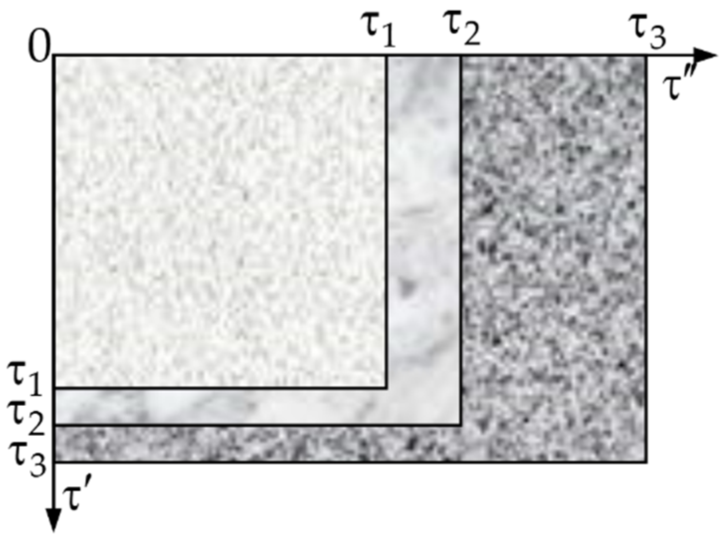
In this case, the integration region is a rectangle that enlarges with growth τ. If α > 1 then the side length of this rectangle along the axis Oτ″ is always α times greater than the side length along the axis Oτ′. Then with increasing τ, the region of integration increases in two coordinates, but with a greater rate along the axis Oτ″ (Figure 13).

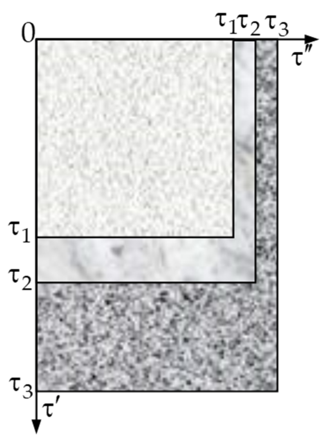
If α < 1 then the side length of this rectangle along the axis Oτ″ is always α times less than the side length along the axis Oτ′. Then with increasing τ, the region of integration increases in two coordinates, but with a greater rate along the axis Oτ′ (Figure 14).

When applying this method here and hereafter, under constructing a grid, it is not necessary to take into account the type of function g(τ), i.e., a rectangular grid can be overlayed in different combinations. We will abide by the structure of the function g(τ) when constructing the grid.

Let n(τ) = αm(τ). Then Formula (22) is modified to the form

$${\displaystyle \underset{0}{\overset{\mathsf{\tau }}{\int }}{\displaystyle \underset{0}{\overset{\alpha \mathsf{\tau }}{\int }}f({\mathsf{\tau }}^{\prime },{\mathsf{\tau }}^{″},\mathsf{\tau })}d{\mathsf{\tau }}^{″}d{\mathsf{\tau }}^{\prime }}\approx {\displaystyle \sum _{i=1}^{\left[n(\mathsf{\tau })\right]}{\displaystyle \sum _{j=1}^{\left[n(\mathsf{\tau })/\alpha \right]}{h}_n^2 f({{\mathsf{\tau }}^{\prime }}_i,{{\mathsf{\tau }}^{″}}_j,\mathsf{\tau })}}$$

The application of this formula is implemented to calculate the integral ${\displaystyle \underset{0}{\overset{\mathsf{\tau }}{\int }}{\displaystyle \underset{0}{\overset{\alpha \mathsf{\tau }}{\int }}{\mathsf{\tau }}^{\prime }{\mathsf{\tau }}^{″}d{\mathsf{\tau }}^{\prime }d{\mathsf{\tau }}^{″}}}$. The results of the calculations are shown in

Table 14. Calculation of integral ${\displaystyle \underset{0}{\overset{\mathsf{\tau }}{\int }}{\displaystyle \underset{0}{\overset{\alpha \mathsf{\tau }}{\int }}{\mathsf{\tau }}^{\prime }{\mathsf{\tau }}^{″}d{\mathsf{\tau }}^{\prime }d{\mathsf{\tau }}^{″}}}$ for α > 1.

n(τ)	m(τ)	h	τ	ατ	Ianalyt	Inum	|Ianalyt − Inum|	E(τ)
104	1.2 × 104	0.0001	1	1.2	0.36	0.359928001101	7.199889950002 × 10−5	0.00019999694305563
2 × 104	2.4 × 104	0.0001	2	2.4	5.76	5.759424004401	0.000575995599001	9.99992359377497 × 10−5
3 × 104	3.6 × 104	0.0001	3	3.6	29.16	29.158056009901	0.001943990098486	6.66663271085926 × 10−5
4 × 104	4.8 × 104	0.0001	4	4.8	92.16	92.155392017602	0.004607982397975	4.99998090058159 × 10−5
5 × 104	6 × 104	0.0001	5	6	225	224.9910000275	0.00899997249754	3.99998777668455 × 10−5
6 × 104	7.2 × 104	0.0001	6	7.2	466.56	466.5444480396	0.015551960396756	3.33332484498378 × 10−5
7 × 104	8.4 × 104	0.0001	7	8.4	864.36	864.3353040539	0.024695946096658	2.85713662092863 × 10−5
8 × 104	9.6 × 104	0.0001	8	9.6	1474.56	1474.5231360704	0.036863929596676	2.49999522546903 × 10−5
9 × 104	1.08 × 105	0.0001	9	10.8	2361.96	2361.9075120891	0.052487910894209	2.22221844968627 × 10−5
105	1.2 × 105	0.0001	10	12	3600	3599.92800011	0.071999889997197	1.99999694436659 × 10−5
1.1 × 105	1.32 × 105	0.0001	11	13.2	5270.76	5270.6641681331	0.095831866897384	1.81817929287966 × 10−5
1.2 × 105	1.44 × 105	0.0001	12	14.4	7464.96	7464.8355841583	0.124415841606742	1.6666645448434 × 10−5
1.3 × 105	1.56 × 105	0.0001	13	15.6	1.0282 × 104	1.0281802 × 104	0.158183814097506	1.5384597304162 × 10−5
1.4 × 105	1.68 × 105	0.0001	14	16.8	1.38298 × 104	1.3829562 × 104	0.197567784391717	1.42856986955462 × 10−5
1.5 × 105	1.8 × 105	0.0001	15	18	1.8225 × 104	1.8224757 × 104	0.242999752483158	1.33333197521623 × 10−5

for α > 1 and in

Table 15. Calculation of integral ${\displaystyle \underset{0}{\overset{\mathsf{\tau }}{\int }}{\displaystyle \underset{0}{\overset{\alpha \mathsf{\tau }}{\int }}{\mathsf{\tau }}^{\prime }{\mathsf{\tau }}^{″}d{\mathsf{\tau }}^{\prime }d{\mathsf{\tau }}^{″}}}$ for α < 1.

n(τ)	m(τ)	h	τ	ατ	Ianalyt	Inum	|Ianalyt − Inum|	E(τ)
104	8000	0.0001	1	0.8	0.16	0.159967999101	3.200089950003 × 10−5	0.00020000562187521
2 × 104	1.6 × 104	0.0001	2	1.6	2.56	2.559743996401	0.000256003599	0.00010000140585941
3 × 104	2.4 × 104	0.0001	3	2.4	12.96	12.9591359919	0.000864008098498	6.66672915508346 × 10−5
4 × 104	3.2 × 104	0.0001	4	3.2	40.96	40.9579519856	0.002048014397987	5.0000351513376 × 10−5
5 × 104	4 × 104	0.0001	5	4	100	99.9959999775	0.004000022497471	4.00002249747133 × 10−5
6 × 104	4.8 × 104	0.0001	6	4.8	207.36	207.3530879676	0.00691203239699	3.33334895688194 × 10−5
7 × 104	5.6 × 104	0.0001	7	5.6	384.16	384.1490239559	0.01097604409664	2.85715433586008 × 10−5
8 × 104	6.4 × 104	0.0001	8	6.4	655.36	655.3436159424	0.016384057596909	2.50000878859085 × 10−5
9 × 104	7.2 × 104	0.0001	9	7.2	1049.76	1049.7366719271	0.023328072896048	2.22222916629024 × 10−5
105	8 × 104	0.0001	10	8	1600	1599.96799991	0.032000089996992	2.00000562481205 × 10−5
1.1 × 105	8.8 × 104	0.0001	11	8.8	2342.56	2342.5174078911	0.042592108891502	1.81818646657938 × 10−5
1.2 × 105	9.6 × 104	0.0001	12	9.6	3317.76	3317.7047038704	0.055296129589091	1.66667057258786 × 10−5
1.3 × 105	1.04 × 105	0.0001	13	10.4	4569.76	4569.6896958479	0.070304152086904	1.53846486657734 × 10−5
1.4 × 105	1.12 × 105	0.0001	14	11.2	6146.56	6146.4721918236	0.087808176383784	1.42857429820557 × 10−5
1.5 × 105	1.2 × 105	0.0001	15	12	8100	8099.8919997975	0.108000202488505	1.33333583319142 × 10−5

for α < 1.

(3)

g(τ) = τ².

In this case, the integration region is also a rectangle that increases with growth τ. Moreover, the growth rate for this region along the axis Oτ″ is much greater than along the axis Oτ′ and the difference between them increases with the increase of τ (Figure 15).

Let n(τ) = (m(τ))² under constructing the variable grid. Then the Formula (22) takes the form

$${\displaystyle \underset{0}{\overset{\mathsf{\tau }}{\int }}{\displaystyle \underset{0}{\overset{{\mathsf{\tau }}^2}{\int }}f({\mathsf{\tau }}^{\prime },{\mathsf{\tau }}^{″},\mathsf{\tau })}d{\mathsf{\tau }}^{″}d{\mathsf{\tau }}^{\prime }}\approx {\displaystyle \sum _{i=1}^{\left[n(\mathsf{\tau })\right]}{\displaystyle \sum _{j=1}^{\left[\sqrt{n(\mathsf{\tau })}\right]}{h}_n^2 f({{\mathsf{\tau }}^{\prime }}_i,{{\mathsf{\tau }}^{″}}_j,\mathsf{\tau })}}.$$

The application of this formula is implemented to the calculation of the integral ${\displaystyle \underset{0}{\overset{\mathsf{\tau }}{\int }}{\displaystyle \underset{0}{\overset{{\mathsf{\tau }}^2}{\int }}{\mathsf{\tau }}^{\prime }{\mathsf{\tau }}^{″}d{\mathsf{\tau }}^{\prime }d{\mathsf{\tau }}^{″}}}$ (

Table 16. Calculation of integral ${\displaystyle \underset{0}{\overset{\mathsf{\tau }}{\int }}{\displaystyle \underset{0}{\overset{{\mathsf{\tau }}^2}{\int }}{\mathsf{\tau }}^{\prime }{\mathsf{\tau }}^{″}d{\mathsf{\tau }}^{\prime }d{\mathsf{\tau }}^{″}}}$.

n(τ)	m(τ)	h	τ	τ2	Ianalyt	Inum	|Ianalyt − Inum|	E(τ)
104	104	0.0001	1	1	0.25	0.2499500000005	4.99999995 × 10−5	0.00019999999800015
1.5 × 104	2.25 × 104	0.0001	1.5	2.25	2.84765625	2.84727657060061	0.00037967939939	0.00013333048867551
2 × 104	4 × 104	0.0001	2	4	16	15.998400030001	0.00159996999897	9.999812493585 × 10−5
2.5 × 104	6.25 × 104	0.0001	2.5	6.25	61.03515625	61.0302735195325	0.0048827304675	7.999865597957 × 10−5
3 × 104	9 × 104	0.0001	3	9	182.25	182.237850180001	0.01214981999854	6.66656790043 × 10−5
3.5 × 104	1.225 × 105	0.0001	3.5	12.25	459.56640625	459.540145657033	0.0262605929666	5.71421074506 × 10−5
4 × 104	1.6 × 105	0.0001	4	16	1024	1023.9488006	0.05119939999953	4.99994140621 × 10−5
4.5 × 104	2.025 × 105	0.0001	4.5	20.25	2075.94140625	2075.84914316203	0.09226308796889	4.44439750039 × 10−5
5 × 104	2.5 × 105	0.0001	5	25	2500	2499.87500152251	0.12499847749481	4.99993909979 × 10−5
5.5 × 104	3.025 × 105	0.0001	5.5	30.25	6920.16015625	6919.90851627453	0.25163997547092	3.63633167137 × 10−5
6 × 104	3.6 × 105	0.0001	6	36	1.1664 × 104	11663.61120315	0.38879685001047	3.33330632725 × 10−5
6.5 × 104	4.225 × 105	0.0001	6.5	42.25	1.885472266 × 104	1.8854142515 × 104	0.58014095548511	3.07689996859 × 10−5
7 × 104	4.9 × 105	0.0001	7	49	2.941225 × 104	2.9411409656 × 104	0.8403441200813	2.85712286575 × 10−5
7.5 × 104	5.625 × 105	0.0001	7.5	56.25	4.44946289 × 104	4.449344239 × 104	1.18651566808313	2.6666492052 × 10−5
8 × 104	6.4 × 105	0.0001	8	64	6.5536 × 104	6.553436161 × 104	1.63838992020585	2.4999846195 × 10−5

).

(4)

g(τ) = $\frac{1}{\mathsf{\tau }}$, $\mathsf{\tau }\ne 0$.

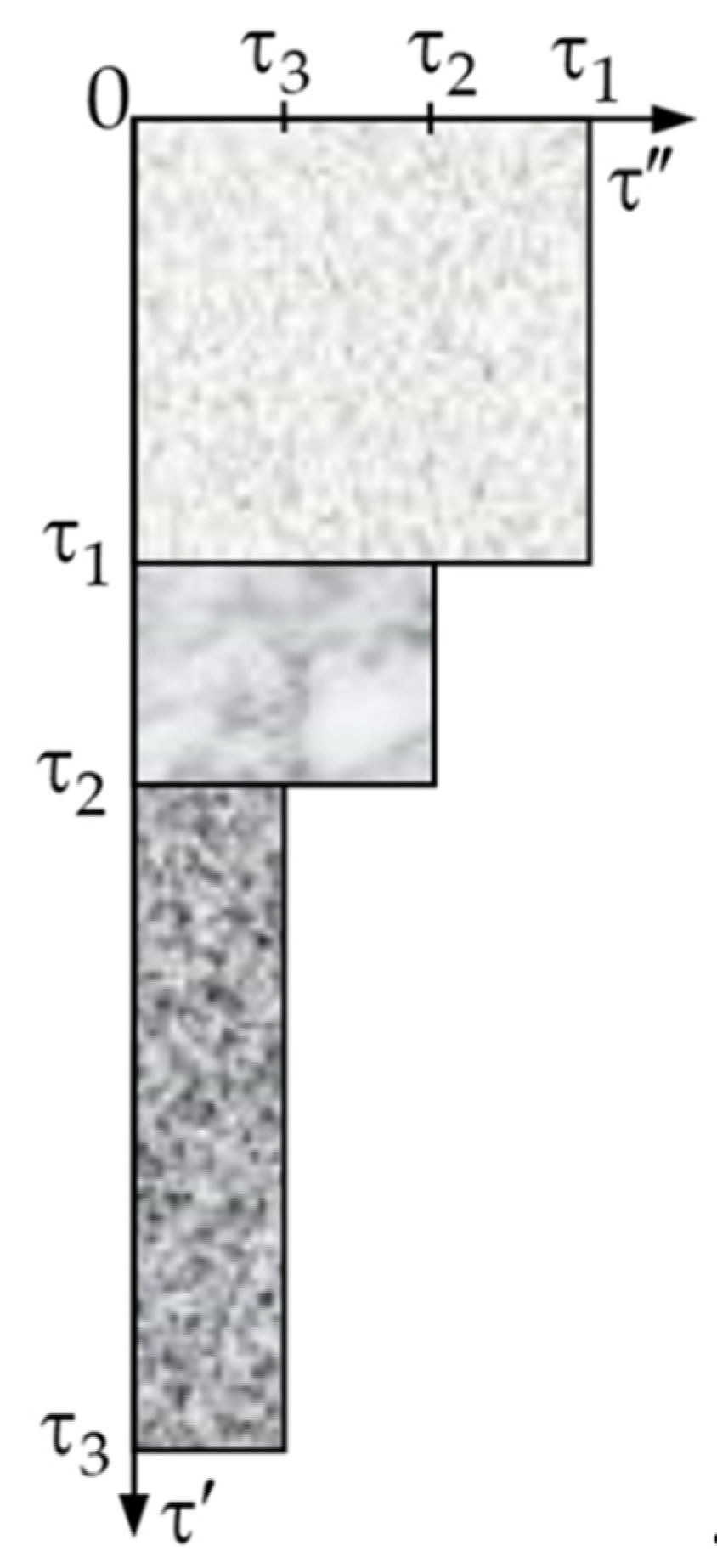
In this case, the integration region is also a rectangle that changes with growth τ. The integration region increases proportionally along the axis Oτ′ and decreases along the axis Oτ″ (Figure 16).

If at constructing the grid we choose a variable number of elements according to the type of function g(τ), i.e., for this case n(τ) = τm(τ), then with increasing τ the number of elements increases along the axis Oτ′, and decreases along the axis Oτ″ according to the change of the integration region. Then at each step, an additional check of the condition m(τ) ≥ 1 (or n(τ)/τ ≥ 1) is required, as there must be at least one grid element along the axis Oτ″.

For this case, we carry out the calculation of integrals by the formula

$${\displaystyle \underset{0}{\overset{\mathsf{\tau }}{\int }}{\displaystyle \underset{0}{\overset{1/\mathsf{\tau }}{\int }}f({\mathsf{\tau }}^{\prime },{\mathsf{\tau }}^{″},\mathsf{\tau })}d{\mathsf{\tau }}^{″}d{\mathsf{\tau }}^{\prime }}\approx {\displaystyle \sum _{i=1}^{\left[n(\mathsf{\tau })\right]}{\displaystyle \sum _{j=1}^{\left[n(\mathsf{\tau })/\mathsf{\tau }\right]}{h}_n^2 f({{\mathsf{\tau }}^{\prime }}_i,{{\mathsf{\tau }}^{″}}_j,\mathsf{\tau })}}.$$

Its application was realized for the calculation of the integral ${\displaystyle \underset{0}{\overset{\mathsf{\tau }}{\int }}{\displaystyle \underset{0}{\overset{1/\mathsf{\tau }}{\int }}{\mathsf{\tau }}^{\prime }{\mathsf{\tau }}^{″}d{\mathsf{\tau }}^{\prime }d{\mathsf{\tau }}^{″}}}$ (

Table 17. Calculation of integral ${\displaystyle \underset{0}{\overset{\mathsf{\tau }}{\int }}{\displaystyle \underset{0}{\overset{1/\mathsf{\tau }}{\int }}{\mathsf{\tau }}^{\prime }{\mathsf{\tau }}^{″}d{\mathsf{\tau }}^{\prime }d{\mathsf{\tau }}^{″}}}$.

n(τ)	m(τ)	h	τ	1/τ	Ianalyt	Inum	|Ianalyt − Inum|	E(τ)
104	104	0.0001	1	1	0.25	0.2499500000005	4.99999995000368 × 10−5	0.000199999998000147
1.5 × 104	6.667 × 104	0.0001	1.5	0.666667	0.25	0.249966662152403	3.33378475972569 × 10−5	0.000133351390389028
2 × 104	5 × 104	0.0001	2	0.5	0.25	0.249974990626	2.50093740000442 × 10−5	0.000100037496000177
2.5 × 104	4 × 104	0.0001	2.5	0.4	0.25	0.24997998477625	2.00152237500155 × 10−5	8.00608950000621 × 10−5
3 × 104	3.333 × 104	0.0001	3	0.333333	0.25	0.249983311108111	1.6688891889241 × 10−5	6.6755567556964 × 10−5
3.5 × 104	2.851 × 104	0.0001	3.5	0.285714	0.25	0.249985683863483	1.43161365165711 × 10−5	5.72645460662842 × 10−5
4 × 104	2.5 × 104	0.0001	4	0.25	0.25	0.24998746015825	1.25398417499468 × 10−5	5.01593669997873 × 10−5
4.5 × 104	2.222 × 104	0.0001	4.5	0.222222	0.25	0.24998883837947	1.11616205303462 × 10−5	4.4646482121385 × 10−5
5 × 104	2 × 104	0.0001	5	0.2	0.25	0.2499899376025	1.00623974999731 × 10−5	4.02495899998926 × 10−5
5.5 × 104	1.818 × 104	0.0001	5.5	0.181818	0.25	0.249990833536177	9.1664638230205 × 10−6	3.6665855292082 × 10−5
6 × 104	1.667 × 104	0.0001	6	0.166667	0.25	0.24999157666707	8.42333292975208 × 10−6	3.36933317190083 × 10−5
6.5 × 104	1.538 × 104	0.0001	6.5	0.153846	0.25	0.249992202066328	7.79793367231825 × 10−6	3.1191734689273 × 10−5
7 × 104	1.429 × 104	0.0001	7	0.142857	0.25	0.249992734599321	7.26540067850518 × 10−6	2.90616027140207 × 10−5
7.5 × 104	1.333 × 104	0.0001	7.5	0.133333	0.25	0.249993192686191	6.80731380930144 × 10−6	2.72292552372058 × 10−5
8 × 104	1.25 × 104	0.0001	8	0.125	0.25	0.249993590043062	6.40995693757569 × 10−6	2.56398277503028 × 10−5

).

In our opinion, for this case of the type of function g(τ) it is advisable to choose the construction of the grid in the case C1 with the correct (appropriate) choice of function m(τ) and step h_m(τ).

If the function g(τ) is periodic (for example g(τ) = sin(τ)), then the region of integration is variable and rectangular. At the intervals of this function increasing, the integration region increases along the axis Oτ″, and at the intervals of decrease, it decreases along the axis Oτ″, respectively. That is, the increasing and decreasing of the integration region have cyclical (periodic) nature. Then the variable integration grid must be chosen by the case C1 with the choice of suitable periodic functions as m(τ) and h_m(τ).

6. Conclusions and Perspectives

All obtained results are new. The numerical method for calculating doubles integrals with variable upper limits was developed. It can be divided into several stages as determining the variable region of integration; overlaying the square or rectangular grid on the integration region; separating the integration subregions consisting of square and triangular elements; applying the cubatures in the subregion with square elements; triangulation partition along variable boundary; calculating the volumes of elementary elements with triangular basis, calculating the reference integral and establishing the calculation error.

The variable region of integration leads to the necessity to change the grid of its division into elementary volumes. The variable of the upper limit of the external integral has a significant effect. Here we consider three cases of a possible change of the grid, namely when this variable changes, we change only the size of the imposed grid and fix the number of partition elements; only the number of division elements changes, and the grid size is fixed, as well as both the number of division elements and the grid size change under fixing their multiplication. In the latter case, we considered an assignment of increasing and decreasing functions describing the change in the number of integration nodes on specific examples. In all considered examples of the application of the proposed method the smallest values of absolute and relative errors are reached for the case of an increase of the number of division elements changes and the grid size is fixed. At the same time, the question remains whether the choice of the function of the number of integration nodes, which increases much more sharply, will give rise to descent the error of the method. Additionally, note that the imposition of a variable grid on the integration region, if necessary, can be applied to definite double integrals.

When finding the estimate of the error of the method, we expanded the integral itself into a Taylor series using Barrow’s theorem. If we impose the definite limits of integration, the obtained formula will be reduced to the classical formula for expanding an integrand into the Taylor series. It is also necessary to carry out an individual investigation on the influence of setting variables of the number of elements of the division of the integration region and the size of the grid on the error estimate.

In this paper, we have considered the case when a double integral with variable limits can be reduced to an integral with simple variables in the upper limits of integration and zero lower limits. However, the proposed changes of variables are not always appropriate. Therefore, further research is needed on numerical integration, which limits functions, including the establishment of conditions and constraints on these functions, the integrand, and the variable region of integration that will be formed.