Tutorial

Harnessing Entropy via Predictive Analytics to Optimize Outcomes in the Pedagogical System: An Artificial Intelligence-Based Bayesian Networks Approach

by
Meng-Leong HOW
* and
Wei Loong David HUNG
National Institute of Education, Nanyang Technological University, Singapore 639798, Singapore
*
Author to whom correspondence should be addressed.
Educ. Sci. 2019, 9(2), 158; https://doi.org/10.3390/educsci9020158
Submission received: 8 May 2019 / Revised: 3 June 2019 / Accepted: 19 June 2019 / Published: 25 June 2019
(This article belongs to the Special Issue Emerging Technologies in Education)

Abstract

:
Educational stakeholders would be better informed if they could use their students’ formative assessments results and personal background attributes to predict the conditions for achieving favorable learning outcomes, and conversely, to gain awareness of the “at-risk” signals to prevent unfavorable or worst-case scenarios from happening. It remains, however, quite challenging to simulate predictive counterfactual scenarios and their outcomes, especially if the sample size is small, or if a baseline control group is unavailable. To overcome these constraints, the current paper proffers a Bayesian Networks approach to visualize the dynamics of the spread of “energy” within a pedagogical system, so that educational stakeholders, rather than computer scientists, can also harness entropy to work for them. The paper uses descriptive analytics to investigate “what has already happened?” in the collected data, followed by predictive analytics with controllable parameters to simulate outcomes of “what-if?” scenarios in the experimental Bayesian Network computational model to visualize how effects spread when interventions are applied. The conceptual framework and analytical procedures in this paper could be implemented using Bayesian Networks software, so that educational researchers and stakeholders would be able to use their own schools’ data and produce findings to inform and advance their practice.

1. Introduction

When efforts are exerted by a student to learn, or by a teacher to teach, it would not be unreasonable to assume that not all of that “energy” would be converted directly into the educational outcomes that they want. Clausius [1] asserts that when work is done (energy expended) on a particular entity inside a system to transform it from one state to another, not all of that energy would be converted and used to change the state of that entity. Some amount of that energy would be “spread out” into other parts of the system. Clausius refers to this “spread” of energy as entropy. The current paper proffers a Bayesian approach in which entropy could be utilized to make improvements in a pedagogical system. For the purpose of illustrating how the concept of entropy could be incorporated in the Bayesian Network analyses, pedagogical entropy refers to an entity’s propensity to change from an ordered state to a disordered state (or a less ordered state) in a pedagogical system. A pedagogical system refers to an education-related system, such as a school. Expounding upon the concept of entropy, in a pedagogical system, work done (for example, efforts exerted in a class intervention by the teacher, or by an after-school tutor) on students might not necessarily result in that “energy” being converted fully into the output (for example, higher scores in a formative assessment). It might be tempting to assume that some of those efforts or “energy” were simply lost. However, from the perspective of entropy, that “energy” was not lost. Rather, it was spread out into other parts of the system.
Larson [2] posits that parts of a pedagogical system would perform better if entropy (which he uses to connote the concept of disorder) is limited, and therefore, if a pedagogical system is sufficiently ordered (low entropy), teaching and learning would be accentuated. Nevertheless, for the pedagogical processes to work, there cannot be low entropy throughout the system. The teacher has to initially create “disorder” in the minds of the students so that they feel challenged by the new concept taught by the teacher. Hence, the students not only need a pedagogical system which has an “ordered” environment for them to learn new concepts; it should also be “disordered” enough to challenge what they know. In order for the pedagogical system to be successful, the sources that contribute to disorder in the system have to be reduced. However, the concept of entropy in a pedagogical system has been relatively unexplored in the extant literature, using quantitative data in a manner which can be easily carried out.
The current paper will explore the notion of entropy, specifically, the spread of “energy” in a pedagogical system will be simulated using a Bayesian Network (BN) model. Using the exemplars provided, educational stakeholders who might not be familiar with advanced mathematics would be able to independently analyze their school data, and to harness the concept of entropy to work for them to predict the conditions that might contribute to optimal educational outcomes.

2. Research Problem and Research Questions

Let us imagine that a team of researchers had collected some data about the weather in the previous week, and that they presented the findings of their study with depictions about what had happened in the past. If they did not make any forecast about the weather pattern in the future, wouldn’t it feel as if their work was incomplete? Now, let us imagine that a team of educational researchers had collected data from a school about the students’ background information and the results of their formative assessments. The researchers would be able to analyze and present the findings of what had transpired in the past from the educational data about how certain aspects of the students’ activities (the inputs) might affect their scores in the formative assessments (the outputs). However, wouldn’t it be more useful if the study could provide some predictive insights that might inform educational practice or policy making amidst uncertainty? A school can be regarded to be a complex system in an educational setting, and entropy is abound in every complex system [3]. If researchers could predict conditions of complex weather systems by utilizing the concept of entropy [4,5,6,7], wouldn’t it also be possible to harness entropy to work for educational stakeholders to predict conditions and outcomes in the future? Specifically, “would it be possible to predict conditions that could enhance student performance, when there could be dynamic confounding factors with parameters that could change?” and “how do these shifting conditions mediate student achievement in their formative assessments?” are two intriguing questions that might interest educational stakeholders, policy makers, and educational researchers [8,9]. Hence, the current paper will be guided by these two research questions.
A situation sometimes faced by educational researchers is that the school might only agree to provide the researchers with access to a small number of students for participation in a study. There might be no students available for a control group, as the school might not wish to provide one, because they would want all the participating students to be inside the treatment group so that they could all benefit from the educational program. Even if a control group could be available for comparison in the post-test vis-à-vis the pre-test assessment, if the quality of the caliber of the small number of participants is high, there might be difficulty in getting statistically significant results using a frequentist approach of measuring gains by comparing results from the post-test to the pre-test [10]. It would also be unrealistic to compare the two groups of students in the treatment group and the control group with each other, as they would be different students with non-identical individual sets of prior knowledge, taught by teachers with perhaps slightly dis-similar methods which might inadvertently contribute to different outcomes in the learning processes and in the performance of the students in the formative assessments. However, even without the use of pre- and post-test results, the notion of entropy could still be explored in a pedagogical system. To overcome these constraints, a Bayesian approach that would be useful to educational research will be presented in the current paper.

3. Definition of Entropy in the Pedagogical System in the Context of This Study

Following the First Law of Thermodynamics, and the concept of free energy [11,12], through the scholastic lens of entropy, when a component of the pedagogical system is observed to be losing “goal-oriented energy” (for example, the “energy” oriented toward achieving the goal of scoring well in the formative assessments), that may be regarded as a movement or displacement of the energy’s location. That energy is neither lost nor destroyed, as energy is always perfectly conserved. For example, the goal-oriented energy that was once localized to a node in the Bayesian Network (BN) that contributes to the goal of achieving high-level scores might disperse into the surrounding nodes that are not goal-oriented (or less goal-oriented).
In this study, the notion of entropy can also be regarded as the propensity for a pedagogical system’s goal-oriented outcome to regress to a lower-level (e.g., from high-level to mid-level, or from mid-level to low-level) when the inputs into the pedagogical system remain unaltered. In accordance with the Second Law of Thermodynamics, entropy can also be used to measure the changes in the pedagogical system, in terms of the transformation of the energy shifting from an aspect which is education goal-oriented to one which is less education goal-oriented. This spread of “energy” within a pedagogical system will be explored via a Bayesian Network in the current paper.

4. Rationale for Using the Bayesian Network Analytical Approach for Educational Research

This section will attempt to provide a preamble to the study by briefly describing the Bayesian theorem and Bayesian Networks. Interested readers who wish to learn more about research in BN are strongly encouraged to consider perusing the works of, for example, Cowell, Dawid, Lauritzen, and Spiegelhalter [13]; Jensen [14]; and Korb & Nicholson [15]. The mathematical formula (see Equation (1)) on which a Bayesian Network was based upon, was developed and first mentioned in 1774 by the mathematician and theologian, Reverend Thomas Bayes [16].
P ( H | E ) = P ( E | H ) . P ( H ) P ( E )
In Equation (1), H represents a hypothesis, and E represents a piece of given evidence. P(H|E) is known as the conditional probability of the hypothesis H, that is, the likelihood of H occurring given the condition that the evidence E is true. This is also referred to as the posterior probability, that is, the probability of the hypothesis H being true after taking into consideration how the evidence E influences the occurrence of the hypothesis H.
P(H) and P(E) represent the probabilities of observing the likelihood of the hypothesis H occurring, and of the likelihood of the evidence E occurring respectively, independent of each other. This is referred to as the prior or marginal probability P(H) and P(E), respectively. P(E|H) represents the conditional probability of the evidence E, that is, the likelihood of E occurring, given the condition that the hypothesis H is true. The quotient P(E|H)/P(E) represents the support which the evidence E provides for the hypothesis H.
It wasn’t until the late 1980s when Bayesian Networks was put forth by Judea Pearl [17] did it become more feasible to utilize them for modeling within the context of social and behavioral science [18,19], especially for analyzing counterfactual scenarios [20], which is important for computational simulations. More recently in the field of education, researchers have also been advancing the Bayesian approach [21,22,23,24,25], because the Bayesian paradigm does not assume or require normal distributions as underlying parameters of a model. Therefore, it is well suited for analyzing data from nonparametric sample sizes [10,26,27,28].
To demonstrate how Bayesian modeling could be done using an educational dataset, and subsequently, how the simulation of hypothetical counterfactual scenarios could potentially inform the practices of educational stakeholders, the results will be presented using the following two segments of analytics:
  • “What has already happened?” descriptive analytics in Section 5:
  • Purpose: To use descriptive analytics to discover from the collected data, the baseline state of the students, and the underlying contributing attributes which drive it.
  • “What-If?” predictive analytics to explore the spread of energy in a pedagogical system in Section 6:
  • Purpose: to use predictive analytics to perform in-silico experiments with fully controllable parameters to predict future entropic outcomes (how “energy” could spread from one part of a pedagogical system to different parts) to better inform educators and policy makers about the key drivers of the attributes that could contribute to conditions required for favorable outcomes, and conversely, become aware of the “at-risk” signals which could prevent unfavorable and worst-case scenarios from happening in the students’ formative assessments.

5. Descriptive Analytics to Find Out “What Has Happened?” in The Pedagogical System

5.1. The Dataset from the School

The Student Performance Data Set used in this paper can be downloaded from the UCI Machine Learning Repository at https://archive.ics.uci.edu/ml/datasets/student+performance.

5.2. Codebook of the Dataset

In the current paper, the dataset used with permission for analysis was generously made available to the public by the original donors, Cortez and Silva [29] at the UCI Machine Learning Repository [30]. The authors of the current paper added a new “Leverageable” column to the dataset. “Leverageable? = Yes” denotes conditions that could be enacted upon by educational stakeholders to influence the outcome of the students’ performance. “Leverageable? = No” denotes conditions that were beyond the influence of educational stakeholders (see Table 1).

5.3. Software Used: Bayesialab

The software used was Bayesialab version 8.0. The 30-day trial version can be downloaded from http://www.bayesialab.com.
Strongly recommended pre-requisite activity: before proceeding with the exemplars shown in the rest of this paper, it would be greatly beneficial to the reader to become familiar with Bayesialab by downloading and reading the free-of-charge user-guide from http://www.bayesia.com/book/ as it contains the descriptions of the myriad tools and functionalities within the Bayesialab software, which are too lengthy to include in the current paper.

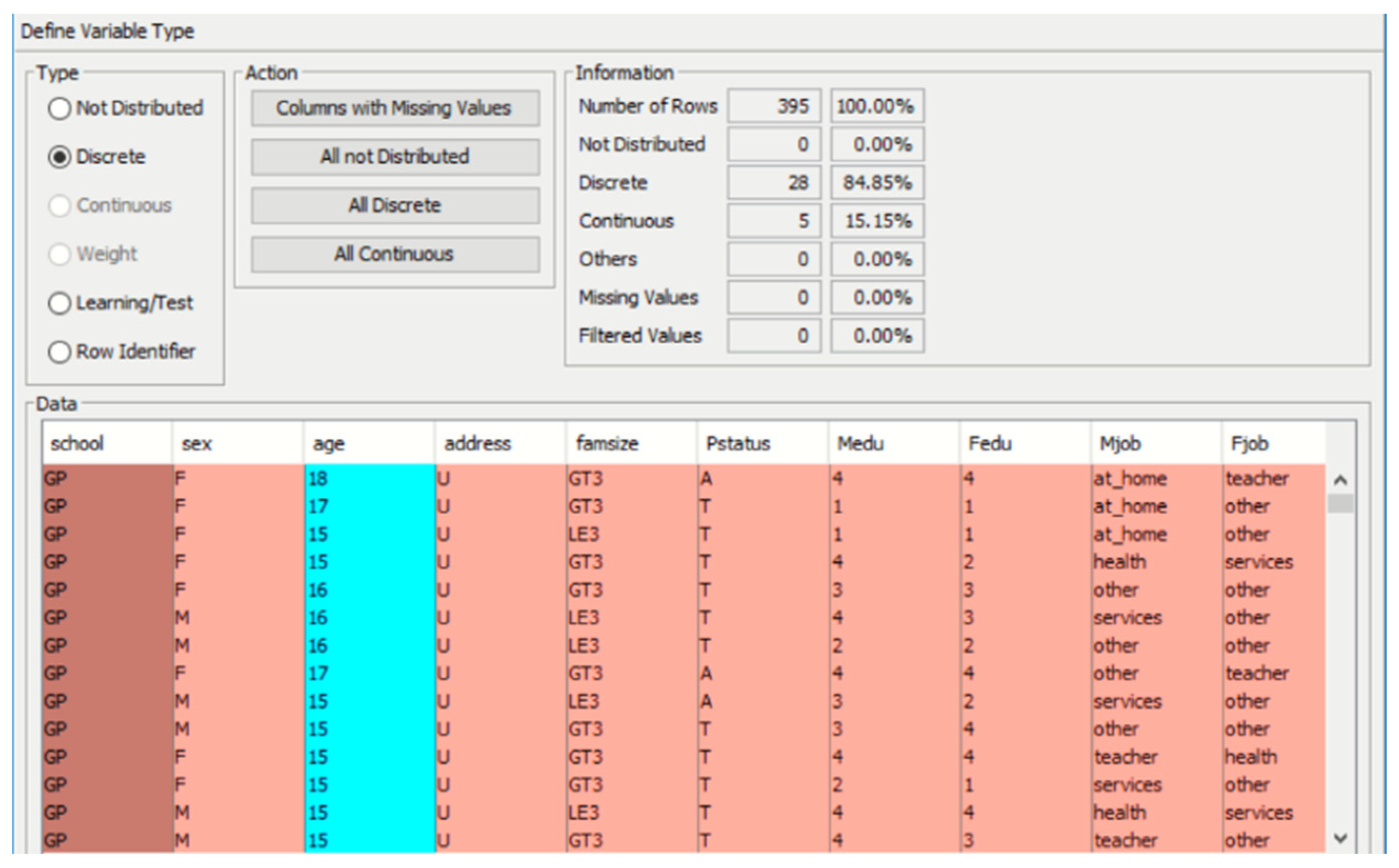
5.4. Pre-Processing: Checking for Missing Values or Errors in the Data

Before using Bayesialab to construct the BN, the first step is to check the data for any anomalies or missing values. In the dataset used in this study, there were no anomalies or missing values (see Figure 1). However, should other researchers encounter missing values in their datasets; rather than discarding the row of data with a missing value, the researchers could use Bayesialab to predict and fill in those missing values. Bayesialab would be able to perform this by machine-learning the overall structural characteristics of that entire dataset being studied, before producing the predicted values. Bayesialab uses the Structural Expectation Maximization (EM) algorithms and Dynamic Imputation algorithms to calculate any missing values [31].

5.5. Discretization of the Dataset

The dataset was then imported into Bayesialab (see Figure 2), and the software automatically tried to categorize the data columns as “discrete” (in beige) or “continuous” (in blue).
Discretization of the continuous data in multiple columns could be automatically performed by the Bayesialab software [32]. The algorithm R2-GenOpt* [33] used in this example (see Figure 3) was the optimal approach recommended by Bayesialab; it was a genetic discretization algorithm for maximizing the coefficient of determination R2 between the discretized variable and its corresponding continuous variable.

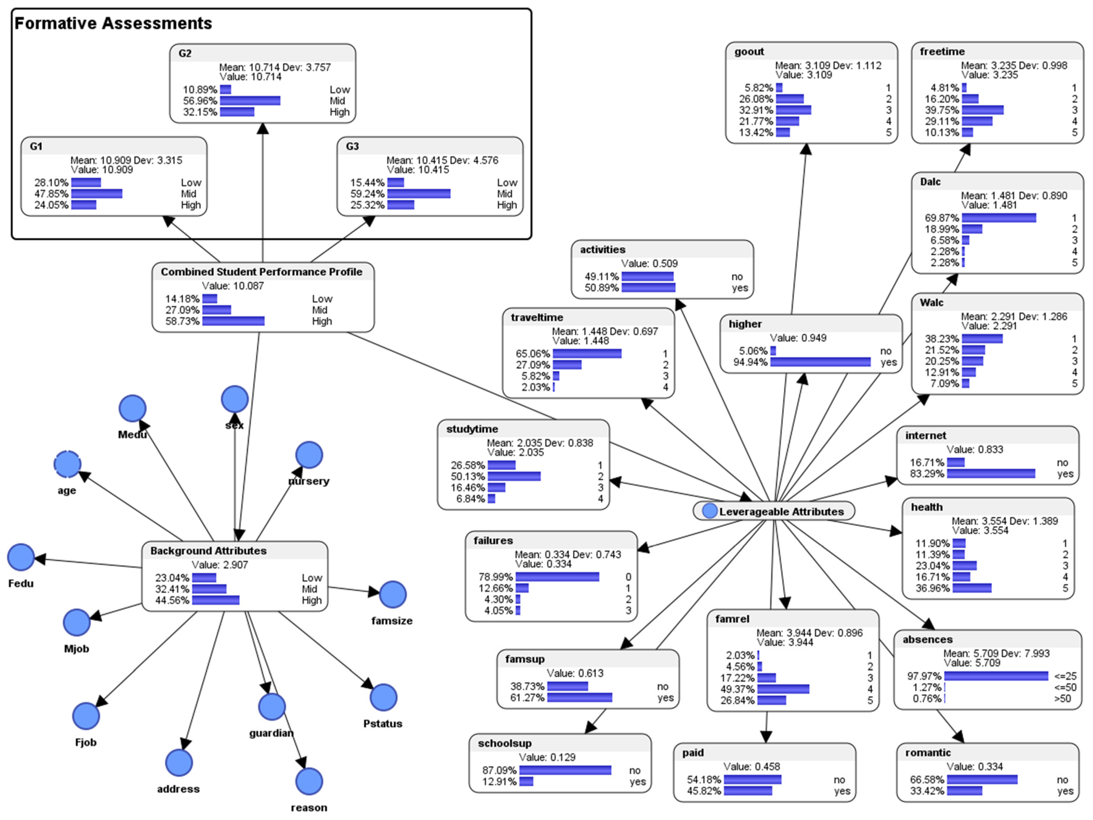
5.6. Descriptive Analytics: Overview of the Bayesian Network Model

Bayesian Networks (BN), also referred to as Belief Networks, Causal Probabilistic Networks, and Probabilistic Influence Diagrams are graphical models which consist of nodes (variables) and arcs or arrows. Each node contains the data distribution of the respective variable. The arcs or arrows between the nodes represent the probabilities of correlations between the variables [34].
As observed in the results (see Figure 4), in the formative assessment G1, 28.10% of the students scored at the Low-level, 47.85% scored at the Mid-level, 24.05% scored at the High-level; in the formative assessment G2, 10.89% of the students scored at the Low-level, 56.96% scored at the Mid-level, 32.15% scored at the High-level; in the final exam G3, 15.44% of the students scored at the Low-level, 56.24% scored at the Mid-level, 25.32% scored at the High-level. The Background Attributes (the non-leverageable attributes in Table 1) could not be influenced by the educational stakeholders. Hence they are held constant in the Bayesian network model.
Among the Leverageable Attributes, the following results were observed:
  • For the attribute (activities) extra-curricular activities, 49.11% responded with “no”; 50.89% responded with “yes.” About half of the students had participated in extra-curricular activities.
  • For the attribute (traveltime) home to school travel time, category 1 represents <15 min., category 2 represents 15 to 30 min., category 3 represents 30 min. to 1 h, and category 4 represents >1 h. 65.06% of the students responded with category 1 (<15 min.); 27.09% responded with category 2 (15 to 30 min.); 5.82% responded with category 3 (30 min. to 1 h); and 2.03% responded with category 4 (> 1 h). A majority of the students (65.06%) spent less than 15 minutes to travel from their homes to school.
  • For the attribute (studytime) weekly study time, category 1 represents <2 h, category 2 represents 2 to 5 h, category 3 represents 5 to 10 h, and category 4 represents >10 h. 26.58% responded with category 1 (< 2 h); 50.13% responded with category 2 (2 to 5 h); 16.46% responded with category 3 (5 to 10 h); and 6.84% responded with category 4 (>10 h). Half of the students spent 2 to 5 hours per week studying, while a quarter spent less than 2 hours per week.
  • For the attribute (failures) number of past class failures, 70.99% of the students had experienced 0 failure; 12.66% had experienced 1 failure; 4.3% had experienced 2 failures; and 4.05% had experienced more than 2 failures. Seven out of ten students did not experience any failure in the past.
  • For the attribute (famsup) family educational support, 38.73% responded with “no”; 61.27% responded with “yes.” Most of the students (61.27%) received educational support from their families.
  • For (schoolsup) extra educational support by the school, 87.09% responded with “no”; 12.91% responded with “yes.” A majority of the students (87.09%) received extra educational support from the school.
  • For the attribute (famrel) quality of family relationships (from 1 which represents “very bad” to 5 which represents “excellent”), 2.03% responded with category 1 (very bad); 4.56% responded with category 2 (bad); 17.22% responded with category 3 (moderate); 49.37% responded with category 4 (good); and 26.84% responded with category 5 (excellent). Nearly half of the students (49.37%) had good relationships with their families, while more than a quarter (26.84%) had excellent relationships.
  • For the attribute (paid) extra paid classes within the course subject, 54.18% responded with “no,” and 45.82% responded with “yes.” More than half (54.18%) of the students did not receive extra paid classes.
  • For the attribute (romantic) with a romantic relationship, 66.58% responded with “no,” and 33.42% responded with “yes.” One-third of the students (33.42%) were in romantic relationships.
  • For the attribute (absences) number of school absences, 97.97% responded with <=25 times; 1.27% responded with <=50 times; and 0.76% responded with >50 times. Almost all the students (except for about 2%) had regular class attendances.
  • For the attribute (health) current health status (from 1 which represents “very bad” to 5 which represents “very good”), 11.90% responded with category 1 (very bad); 11.39% responded with category 2 (bad); 23.04% responded with category 3 (moderate); 16.71% responded with category 4 (good); and 36.96% responded with category 5 (very good). More than one-third of the students reported having very good health.
  • For the attribute (internet) Internet access at home, 16.71% responded with “no,” and 83.29% responded with “yes.” A majority of the students (83.29%) had Internet access at home.
  • For the attribute (Walc) weekend alcohol consumption (from 1 which represents “very low” to 5 which represents “very high”), 38.23% responded with category 1 (very low); 21.52% responded with category 2 (low); 20.25% responded with category 3 (moderate); 12.91% responded with category 4 (high); and 7.09% responded with category 5 (very high). More than one-third (38.23%) of the students consumed a very low level of alcohol during the weekends.
  • For the attribute (Dalc) weekday alcohol consumption (from 1 which represents “very low” to 5 which represents “very high”), 69.87% responded with category 1 (very low); 18.99% responded with category 2 (low); 6.58% responded with category 3 (moderate); 2.28% responded with category 4 (high); and 2.28% responded with category 5 (very high). More than two-thirds (69.87%) of the students consumed a very low level of alcohol during the weekdays.
  • For the attribute (freetime) free time after school (from 1 which represents “very low” to 5 which represents “very high”), 4.81% responded with category 1 (very low); 16.20% responded with category 2 (low); 39.75% responded with category 3 (moderate); 29.11% responded with category 4 (high); and 2.28% responded with category 5 (very high). Almost four in ten students (39.75%) had moderate amount of free time after school.
  • For the attribute (goout) going out with friends, (from 1 which represents “very low” to 5 which represents “very high”), 5.82% responded with category 1 (very low); 26.08% responded with category 2 (low); 32.91% responded with category 3 (moderate); 21.77% responded with category 4 (high); and 13.42% responded with category 5 (very high). Almost one-third of the students (32.91%) had moderate amount of time to go out with their friends.
  • For the attribute (higher) which asked whether the student wished to pursue higher education, 49.11% responded with “no,” and 50.89% responded with “yes.” Slightly more than half of the students (50.89%) wished to pursue higher education.

5.7. Descriptive Analytics: Entropy in the Bayesian Network Model

The entropy of the data distribution within each node of the BN (see Figure 5) can be visualized in Bayesialab (in validation mode) by right-clicking on each node and selecting “Display Expected Log-loss” because entropy is mathematically expressed (see Equation (2)) as:
H ( X ) = x X p ( x ) l o g 2 ( p ( x ) )
Since entropy is the sum the Expected Log-Loss of each state x of variable X when using network B, it can be expressed (see Equation (3)) as:
H ( X ) = x X L L x
where Log-loss can be expressed (see Equation (4)) as:
L L x = p B ( x ) l o g 2 ( p B ( x ) )
The entropy in the pedagogical system can be visualized (see Figure 6) in terms of size and colors by using the mapping tool in Bayesialab (in validation mode) on the menu bar at: Visual > Overall > Mapping > 2D mapping.
The bigger sized nodes suggest that there is higher entropy (more disorder) in them. Conversely, the smaller sized nodes suggest that there is lower entropy (less disorder) in those variables. The Kullback-Leibler [35] divergence values on the lines between the nodes, which measure the directed divergence between the distributions, are used by Bayesialab to represent the strength of the relationships between the nodes. The reasons for higher entropy or lower entropy might not be so obvious at first glance. As mentioned earlier, an environment which has less disorder is conducive to teaching and learning. However, some disorder is also needed to engage and challenge the students into acquiring new knowledge. Therefore, the educational stakeholders might wish to consider focusing on the variables with higher entropy (more disorder), for example, by interviewing the students to collect qualitative data from them to understand more about why they might be experiencing more disorder or challenges in those areas.

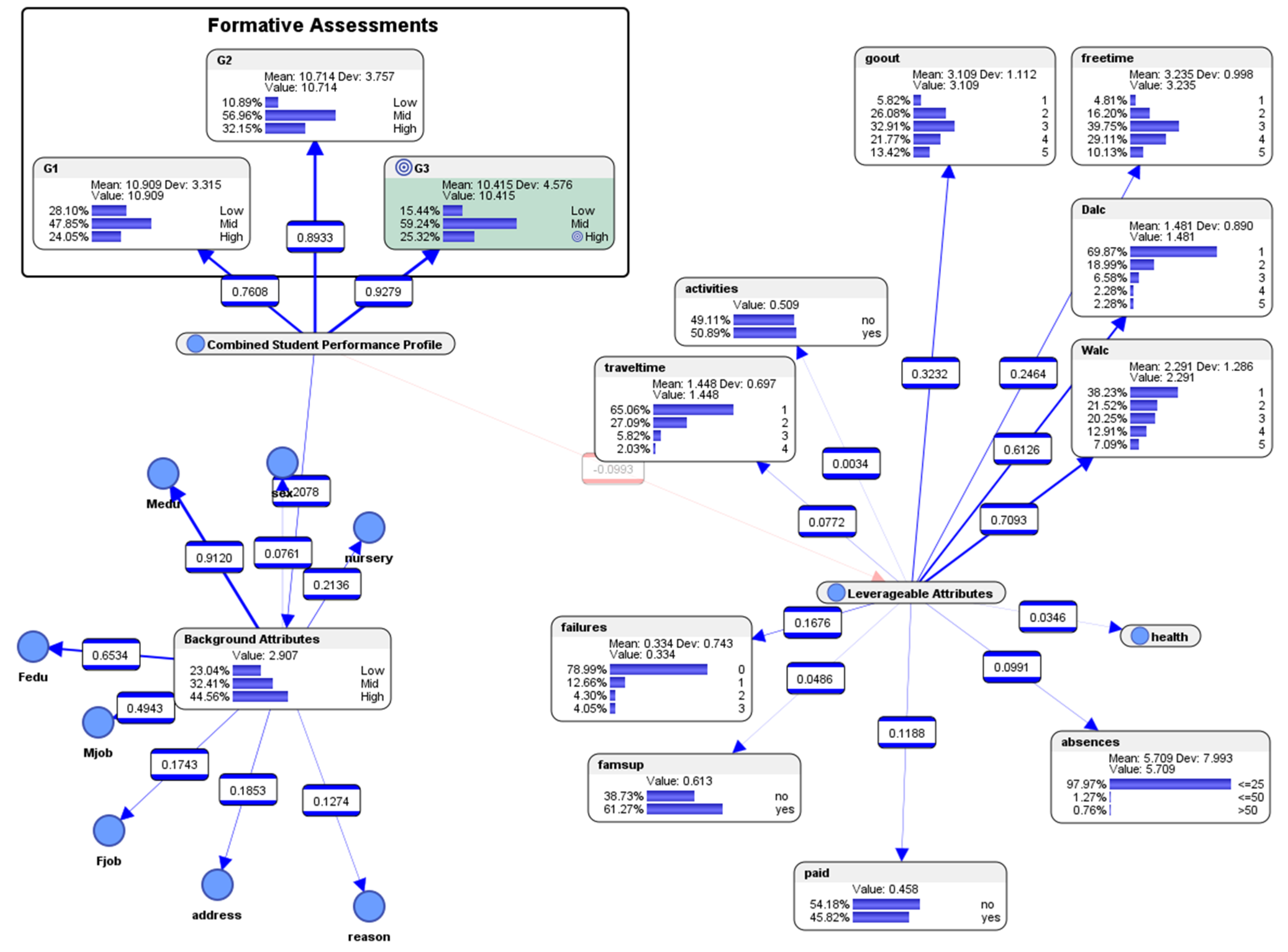
5.8. Descriptive Analytics: Mutual Information in the Bayesian Network Model

The notion of mutual information [36] can be regarded as the reduction in uncertainty about one variable given knowledge of another. High mutual information suggests that there is a large reduction in uncertainty. Low mutual information indicates that there is a small reduction in uncertainty. Zero mutual information between two variables indicates that the variables are independent. Arc Mutual Information is a visual tool that measures the quantity of information shared between the variables connected with an arc. It can be visualized in Bayesialab (in validation mode) via these steps on the menubar: Analysis > Visual > Overall > Arc > Mutual Information.
Inside each box in the middle of each arc (see Figure 7), the following are presented, in case the researcher needs more details about the Mutual Information:
  • Normalized Mutual Information (with respect to the child)
  • Normalized Mutual Information (with respect to the parent)
  • Symmetric Normalized Mutual Information
  • Relative Mutual Information (with respect to the child)
  • Relative Mutual Information (with respect to the parent)
  • Symmetric Relative Mutual Information

5.9. Descriptive Analytics: Pearson Correlation Analysis

To complement the work of colleagues who might prefer to visualize data in terms of frequentist statistics, descriptive analytics can also be performed by using the Pearson correlation analysis tool in Bayesialab. It can be used for corroboration of the relationship analyses between the students’ learning performances in the formative assessments and their background information. The intention is to provide another perspective of looking at the data, just in case the BN approach missed something that might be interesting to the analyst and educational stakeholders. The visualizations of the Pearson correlations can be presented so that it is easier to see the positive correlations highlighted in thicker blue lines (see Figure 8) and negative correlations highlighted in red (see Figure 9). One suggestion for the interpretation of the positive Pearson correlations (see Figure 8) could be, that the thicker blue lines and their corresponding nodes might represent the regions which could potentially impact the students positively. The tool can be activated in Bayesialab (in validation mode) via these steps on the menubar: Analysis > Visual > Overall > Arc > Pearson Correlation > R+ (positive correlations).
One suggestion for the interpretation of the negative Pearson correlations (see Figure 9) could be, that the red lines and nodes might represent the regions which the educational stakeholders ought to be concerned about, as they could potentially impact the students negatively. The tool can be activated in Bayesialab (in validation mode) via these steps on the menubar: Analysis > Visual > Overall > Arc > Pearson Correlation > R- (negative correlations).

5.10. Organization of the Rest of the Paper

In this section, descriptive analytics was used to depict “what had happened?” in the performance levels of the students’ formative assessments, and the conditions which were associated with the outcomes. The following section demonstrates how predictive analytics could be useful to educational stakeholders through the simulations of four “what-if?” scenarios, so that readers can visualize the spreading out of “energy” in a pedagogical system when an intervention (which can be likened to “external energy”) is applied to the pedagogical system.
Subsequently, a section on the evaluation of the predictive performance of the Bayesian network model will be presented using measurement tools such as the Gains curve, the Lift curve, the Receiver Operating Characteristic (ROC) curve, and by performing target evaluation cross-validation by K-Folds. Finally, the implications of using the Bayesian approach for informing the practices of educational stakeholders, and for advancing educational research will be presented in the discussion and conclusion sections.

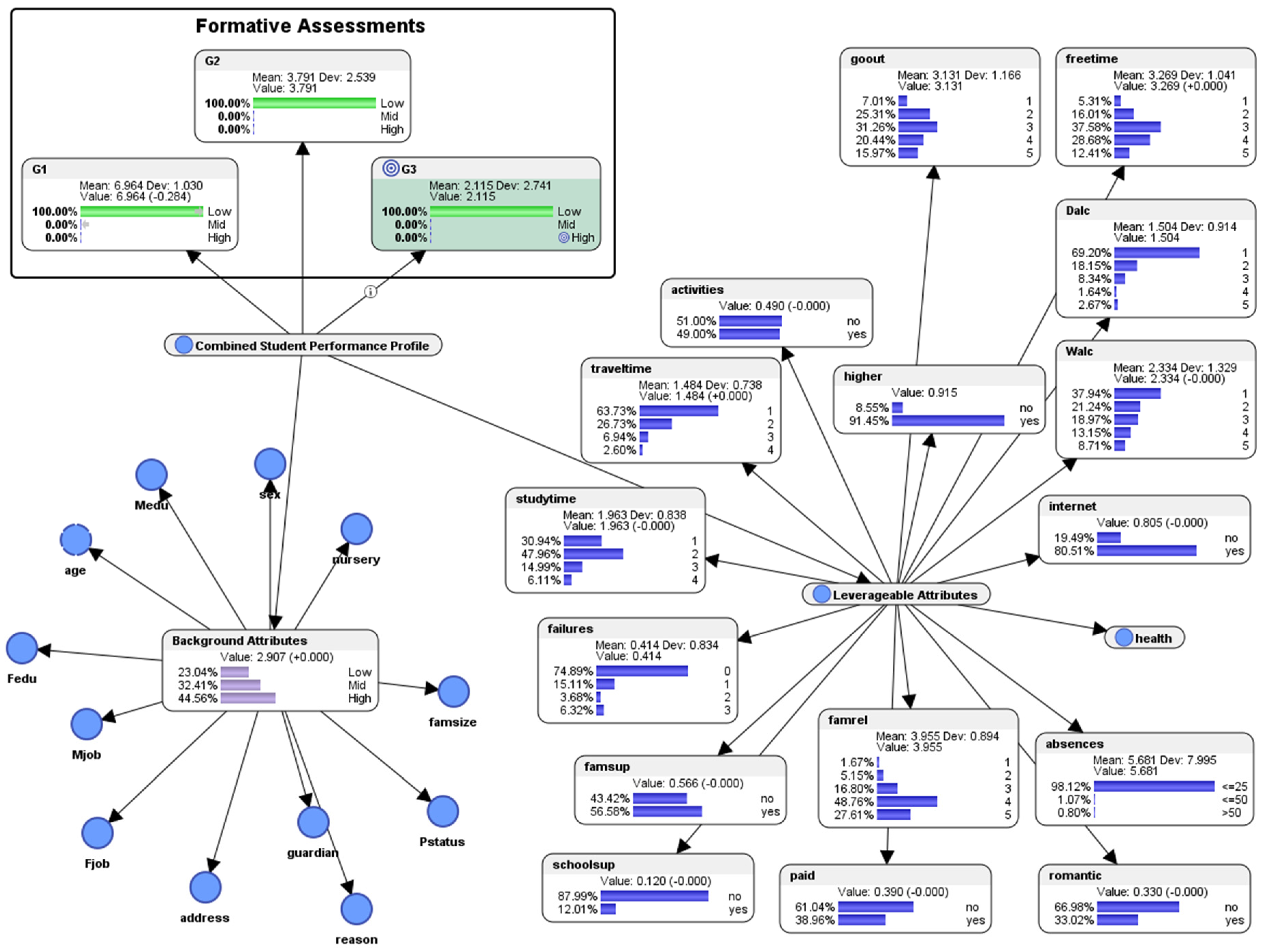
6. Predictive Analytics: Simulation of “What-If?” Scenarios to Visualize the “Spread of Energy” (Entropy) in a Pedagogical System

To demonstrate how the results of the descriptive analytics in Section 5 could be extended upon using predictive analytics to visualize the spread of “energy” within a pedagogical system, the following four hypothetical scenarios will be presented in terms of probability, so that it is more intuitive for educational stakeholders (who are not computational scientists) to comprehend. Admittedly, there is no strict criteria upon which these scenarios are selected out of many possible ones, as this is a purely exploratory exercise.
Hypothetical scenario 1:
What would happen in the formative assessments G1, G2, and final exam G3 if the students go out less with their friends, spend more time studying, minimize their absences from school, and receive extra educational support from their families, as well as extra educational support from their school? How does intervening in one part of the pedagogical system spread out the effects to the other parts?
To simulate the hypothetical scenario (see Figure 10), the leverageable attributes were simulated as follows: “goout” was adjusted to 100% at category 1 (very low); “studytime” was adjusted to 100% at category 4 (>10 h per week); “famsup” was adjusted to 100% in the “yes” category; “schoolsup” was adjusted to 100% in the “yes” category; and “absences” was adjusted to 100% in the “<=25” category.
As observed in the simulation (see Figure 10), in the formative assessment G1, 25.51% of the students counterfactually scored at the Low-level (originally 28.10%), 45.12% counterfactually scored at the Mid-level (originally 47.85%), and 29.37% counterfactually scored at the High-level (originally 24.05%).
In the formative assessment G2, 9.96% of the students counterfactually scored at the Low-level (originally 10.89%), 51.47% counterfactually scored at the Mid-level (originally 56.96%), and 38.57% counterfactually scored at the High-level (originally 32.15%).
In the final exam G3, 14.11% of the students counterfactually scored at the Low-level (originally 15.44%), 54.12% counterfactually scored at the Mid-level (originally 56.24%), and 31.78% counterfactually scored at the High-level (originally 25.32%).
This simulated hypothetical scenario suggests there might be improvements in the formative assessments G1 and G2, and final exam G3 (with more students counterfactually scoring at the High-level) if the students go out less with their friends, spend more time studying, minimize their absences from school, and receive extra educational support from their families, as well as extra educational support from their school.
Hypothetical scenario 2:
What would happen in the formative assessments G1, G2, and final exam G3 if the students go out less with their friends, spend more time studying, minimize their absences from school, while receiving extra educational support from their families, as well as extra educational support from their school, and also receive extra paid classes within the course subject? How does intervening in one part of the pedagogical system spread out the effects to the other parts?
In addition to the adjustments in the leverageable attributes made in hypothetical scenario 1, for the present hypothetical scenario 2, the attribute “paid” was also adjusted to 100% in the “yes” category. As observed in the simulation (see Figure 11), in the formative assessment G1, 25.72% of the students counterfactually scored at the Low-level (compared 25.51% in hypothetical scenario 1; originally at 28.10% in the descriptive analytics), 45.39% counterfactually scored at the Mid-level (compared to 45.12% in hypothetical scenario 1; originally at 47.85% in the descriptive analytics), and 28.89% counterfactually scored at the High-level (compared to 29.37% in hypothetical scenario 1; originally at 24.05% in the descriptive analytics).
In the formative assessment G2, 10.03% of the students counterfactually scored at the Low-level (compared to 9.96% in hypothetical scenario 1; originally at 10.89% in the descriptive analytics), 51.98% counterfactually scored at the Mid-level (compared to 51.47% in hypothetical scenario 1; originally at 56.96% in the descriptive analytics), and 37.99% counterfactually scored at the High-level (compared to 38.57% in hypothetical scenario 1; originally at 32.15% in the descriptive analytics).
In the final exam G3, 14.20% of the students counterfactually scored at the Low-level (compared to 14.11% in hypothetical scenario 1; originally at 15.44% in the descriptive analytics), 54.61% counterfactually scored at the Mid-level (compared to 54.12% in hypothetical scenario 1; originally at 56.24% in the descriptive analytics), and 31.19% counterfactually scored at the High-level (compared to 31.78% in hypothetical scenario 1; originally at 25.32% in the descriptive analytics).
There was a surprisingly unexpected outcome in hypothetical scenario 2: not only did extra paid classes not improve the students’ performance; in the low, mid and high-levels there were respective decreases in performance across G1, G2, and final exam G3. This counterfactual outcome is opposite to the researcher’s initial conventional assumption that paid extra classes would improve the students’ performances in formative assessments. While there was indeed an initial intention to consider the differences between scenario 2 and scenario 1, the findings were purely exploratory and inconclusive, so it would be contrived to calculate the gains by directly subtracting the counterfactual results between scenario 2 and scenario 1.
Exploring the effects of extra paid classes outside school on the student is beyond the scope of the present paper, however, it would be interesting to investigate this in a future study. Readers who are interested in the role that extra paid tutoring plays in contributing to the outcomes of students’ educational assessments may peruse the works of researchers such as Cole [37], Huang [38], Pai, Ho and Lam [39], and Rickard and Mills [40].
Hypothetical scenario 3:
What conditions are required in the leverageable attributes if we wish 100% of the students could score at the high-level in the final exam G3? How does intervening in one part of the pedagogical system spread out the effects to the other parts? As previously mentioned in Section 4 while referring to Equation (1), P(E|H) represents the conditional probability of the evidence E, that is, the likelihood of E occurring, given the condition that the hypothesis H is true. In this context, the BN can be used to simulate counterfactually, that, in order for 100% of the students to score at the High-level in the final exam G3, the following conditions would need to happen in the leverageable attributes (see Figure 12).
For the attribute (activities) extra-curricular activities, it would be ideal if 47.79% respond with “no” (compared to 49.11% originally in the descriptive analytics); and if 52.21% respond with “yes” (compared to 50.89% originally in the descriptive analytics). In other words, a little increase in extra-curricular activities might be beneficial for the students’ performance in the final exam G3, however, more research on this is needed in a future study.
For the attribute (traveltime) home to school travel time, it would be ideal if 66.52% of the students respond with category 1 (<15 min.), compared to the original 65.06% in the descriptive analytics; if 27.67% responded with category 2 (15 to 30 min.), compared to the original 27.09% in the descriptive analytics; if 4.45% respond with category 3 (30 min. to 1 h), compared to the original 5.82% in the descriptive analytics; and if 1.35% respond with category 4 (> 1 h), compared to the original 2.03% in the descriptive analytics. The results suggest that it would be better if travel time from home to school could be shorter.
For the attribute (studytime) weekly study time, it would be ideal if 21.50% of the students could respond with category 1 (< 2 h), compared to the original 26.58% in the descriptive analytics; if 50.45% could respond with category 2 (2 to 5 h), compared to the original 50.13% in the descriptive analytics; if 20.02% could respond with category 3 (5 to 10 h), compared to the original 16.46% in the descriptive analytics; and if 8.04% could respond with category 4 (>10 h), compared to the original 6.84% in the descriptive analytics. The results suggest that it would be ideal if the students could spend more time studying.
For the attribute (failures) number of past class failures, it would be ideal if 83.47% of the students had experienced 0 failure, compared to the original 70.99% in the descriptive analytics; if 10.86% had experienced 1 failure, compared to the original 12.66% in the descriptive analytics; if 3.92% had experienced 2 failures, compared to the original 4.3%; and if 1.76% had experienced more than 2 failures, instead of the original 4.05%. The results suggest that experiencing zero or fewer class failures in the past could contribute to better performance in the final exam G3.
For the attribute (famsup) family educational support, it would be ideal if 36.02% could respond with “no” and if 63.98% could respond with “yes”; compared to the original 38.73% for “no” and the original 61.27% for “yes.” Hence, the results suggest that more family educational support could potentially contribute to better performance in the final exam G3.
For (schoolsup) extra educational support by the school, it would be ideal if 85.87% could respond with “no”; compared to the original 87.09%, and if 14.13% could respond with “yes”; compared to the original 12.91%. The results suggest that more extra educational support by the school could potentially contribute to better performance in the final exam G3.
For the attribute (famrel) quality of family relationships, it would be ideal if 2.05% could respond with category 1 (very bad), compared to the original 2.03%; if 3.56% could respond with category 2 (bad), compared to the original 4.56%; if 16.33% could respond with category 3 (moderate), compared to the original 17.22%; if 49.47% could respond with category 4 (good), compared to the original 49.37%; and if 28.59% could respond with category 5 (excellent), instead of the original 26.84%. The results suggest that a high quality of family relationships could potentially contribute to better performance in the final exam G3.
For the attribute (paid) extra paid classes within the course subject, it would be ideal if 50.93% could respond with “no,” instead of the original 54.18%; and if 49.07% could respond with “yes,” instead of the original 45.82%. The results suggest that more extra paid classes within the course subject could potentially contribute to better performance in the final exam G3.
For the attribute (romantic) “with a romantic relationship,” it would be ideal if 66.29% could respond with “no” compared to the original 66.58%; and if 33.71% could respond with “yes” instead of the original 33.42%. The results suggest that the current level of students in a romantic relationship is already very close to the optimum level that could contribute to the achievement of a high-level of performance in the final exam G3.
For the attribute (absences) number of school absences, it would be ideal if 98.19% could respond with <=25 times (originally 97.97% in the descriptive analytics); if 1.35% could respond with <=50 times (originally 1.27%); and if 0.46% could respond with >50 times (originally 0.76%). The results suggest that fewer number of school absences could contribute to the achievement of a high-level of performance in the final exam G3, which is congruent with the findings of Robinson, Lee, Dearing, and Rogers [41].
For the attribute (health) current health status, the simulated counterfactual results became 12.81% in category 1 “very bad” (originally 11.90% in the descriptive analytics); 10.94% in category 2 “bad” (originally 11.39%); 24.91% in category 3 “moderate” (originally 23.04%); 17.71% in category 4 “good” (originally 16.71%); and 33.63% in category 5 “very good” (originally 36.96%). The original results were already slightly better than the simulated counterfactual results, which suggest that health might not be a potential point of leverage that educational stakeholders could improve to contribute to the achievement of a high-level of performance in the final exam G3.
For the attribute (internet) Internet access at home, it would be ideal if 14.52% could respond with “no” (originally 16.71% in the descriptive analytics) and if 85.48% could respond with “yes” (originally 83.29%). The results suggest that increasing Internet access at home for more students might contribute to the achievement of a high-level of performance in the final exam G3.
For the attribute (Walc) weekend alcohol consumption, the simulated counterfactual results became 46.01% in category 1 “very low” (originally 38.23%); 24.27% in category 2 “low” (originally 21.52%); 17.85% in category 3 “moderate” (originally 20.25%); 8.07% in category 4 “high” (originally 12.91%); and 3.80% in category 5 “very high” (originally 7.09%). The results suggest that lower weekend alcohol consumption would be preferred for achieving a high-level of performance in the final exam G3.
For the attribute (Dalc) weekday alcohol, the simulated counterfactual results became 80.14% in category 1 “very low” (originally 69.87%); 13.45% in category 2 “low” (originally 18.99%); 3.42% in category 3 “moderate” (originally 6.58%); 1.71% in category 4 “high” (originally 2.28%); and 1.28% in category 5 “very high” (originally 2.28%). The results suggest that lower weekday alcohol consumption would be preferred for achieving a high-level of performance in the final exam G3.
For the attribute (freetime) free time after school, the simulated counterfactual results became 5.16% in category 1 “very low” (originally 4.81%); 17.62% in category 2 “low” (originally 16.20%); 42.18% in category 3 “moderate” (originally 39.75%); 28.21% in category 4 “high” (originally 29.11%); and 6.84% in category 5 “very high” (originally 2.28%). The results suggest that slightly higher levels of free time after school might contribute to the achievement of a high-level of performance in the final exam G3. More research is needed to investigate this in future studies.
For the attribute (goout) going out with friends, the simulated counterfactual results became 5.35% in category 1 “very low” (originally 5.82%); 28.91% in category 2 “low” (originally 26.08%); 36.55% in category 3 “moderate” (originally 32.91%); 19.91% in category 4 “high” (originally 21.77%); and 9.27% in category 5 “very high” (originally 13.42%). The results suggest that increasing “moderate” amount of going out with friends, and decreasing “low,” “very low,” “high,” and “very high” amounts of going out with friends might contribute to the achievement of a high-level of performance in the final exam G3. More research is needed to investigate this in future studies.
For the attribute (higher) which asked whether the student wished to pursue higher education, the simulated counterfactual results became 1.75% in the “no” category (originally 49.11% in the descriptive analytics) and 98.25% in the “yes” category (originally 50.89%). The results suggest that this is an important attribute which might contribute to the achievement of a high-level of performance in the final exam G3.
In this section, the simulated conditions in this hypothetical scenario suggested some parameters that might serve as possible discussions for the educational stakeholders for them to achieve the “best-case scenario.” In the next section, the simulation for the “worst-case scenario” will be presented.
Hypothetical scenario 4:
Counterfactually, to simulate the “worst case scenario,” what are the conditions that could be observable in the leverageable attributes, if hypothetically 100% of the students score consistently low in the formative assessments G1, G2, and final exam G3? How does intervening in one part of the pedagogical system spread out the effects to the other parts?
As previously mentioned in Equation (1), P(E|H) represents the conditional probability of the evidence E, that is, the likelihood of E occurring, given the condition that the hypothesis H is true. In this context, the BN can be used to simulate counterfactually, in the “worst case scenario” if 100% of the students score at the low-level in all 3 of the formative assessments G1, G2, and final exam G3, the following warning signs could hypothetically be observed in the leverageable attributes (see Figure 13).
For the attribute (activities) extra-curricular activities, the worst simulated counterfactual results would become 51.13%% in “no” (compared to 49.11% originally in the descriptive analytics); and 48.87% in “yes” (compared to 50.89% originally in the descriptive analytics). The counterfactual results suggest that, a little decrease in extra-curricular activities might not be beneficial for the students’ performance in the formative assessments G1 and G2, and in the final exam G3. However, more research on this is needed in a future study.
For the attribute (traveltime) home to school travel time, the worst counterfactual results would occur if 63.62% of the students respond with category 1 (<15 min.), compared to the original 65.06% in the descriptive analytics; if 26.70% responded with category 2 (15 to 30 min.), compared to the original 27.09% in the descriptive analytics; if 7.04% respond with category 3 (30 min. to 1 h), compared to the original 5.82% in the descriptive analytics; and if 2.64% respond with category 4 (> 1 h), compared to the original 2.03% in the descriptive analytics. The counterfactual results suggest that if travel time from home to school was slightly longer, it might not be beneficial for the students’ performance in the formative assessments G1 and G2, and in the final exam G3, however, more research on this is needed in a future study.
For the attribute (studytime) weekly study time, the worst counterfactual results would occur if 31.30% of the students respond with category 1 (< 2 h), compared to the original 26.58% in the descriptive analytics; if 47.85% respond with category 2 (2 to 5 h), compared to the original 50.13% in the descriptive analytics; if 14.81% respond with category 3 (5 to 10 h), compared to the original 16.46% in the descriptive analytics; and if 6.04% respond with category 4 (>10 h), compared to the original 6.84% in the descriptive analytics. The counterfactual results suggest that if the students spend less time studying, it might not be beneficial for their performance in the formative assessments G1 and G2, and in the final exam G3.
For the attribute (failures) number of past class failures, the worst-case scenario would occur if 74.57% of the students had experienced 0 failure, compared to the original 70.99% in the descriptive analytics; if 15.27% had experienced 1 failure, compared to the original 12.66% in the descriptive analytics; if 3.66% had experienced 2 failures, compared to the original 4.3%; and if 6.50% had experienced more than 2 failures, instead of the original 4.05%. The counterfactual results suggest that experiencing failures in the past could contribute to poor performance in the formative assessments G1 and G2, and in the final exam G3.
For the attribute (famsup) family educational support, the worst-case scenario would occur if 43.72% respond with “no” compared to the original 38.73% for “no” in the descriptive analytics, and if 56.28% respond with “yes” compared to the original 61.27% for “yes” in the descriptive analytics. Hence, the results suggest that less family educational support could potentially contribute to poor performance in the formative assessments G1 and G2, and in the final exam G3.
For (schoolsup) extra educational support by the school, the worst-case scenario would occur if 88.06% respond with “no” compared to the original 87.09% in the descriptive analytics; and if 11.94% respond with “yes” compared to the original 12.91%. The results suggest that less extra educational support by the school could potentially contribute to poor performance in the formative assessments G1 and G2, and in the final exam G3.
For the attribute (famrel) quality of family relationships, the worst-case scenario would occur if 1.66% respond with category 1 (very bad), compared to the original 2.03% in the descriptive analytics; if 5.21% respond with category 2 (bad), compared to the original 4.56%; if 16.81% respond with category 3 (moderate), compared to the original 17.22%; if 48.73% respond with category 4 (good), compared to the original 49.37%; and if 27.59% respond with category 5 (excellent), instead of the original 26.84%. The counterfactual results suggest that lower quality of family relationships could potentially lead to worse performance in the final exam G3.
For the attribute (paid) extra paid classes within the course subject, the worst-case scenario would occur if 61.45% respond with “no” instead of the original 54.18%; and if 38.55% respond with “yes” instead of the original 45.82%. The counterfactual results suggest that fewer extra paid classes within the course subject could potentially lead to poor performance in the formative assessments G1 and G2, and in the final exam G3.
For the attribute (romantic) “with a romantic relationship,” the worst-case scenario would occur if 67.01% respond with “no” compared to the original 66.58%; and if 32.99% respond with “yes” instead of the original 33.42%. The counterfactual results suggest that, interestingly, not being in a romantic relationship might contribute to poor performance in the formative assessments G1 and G2, and in the final exam G3. However, this is inconclusive, so more research might be needed.
For the attribute (absences) number of school absences, the worst-case scenario would occur if 98.12% respond with <=25 times (compared to originally 97.97% in the descriptive analytics); if 1.06% respond with <=50 times (originally 1.27%); and if 0.81% could respond with >50 times (originally 0.76%). The counterfactual results suggest that a slightly higher number of school absences could lead to poor performance in the formative assessments G1 and G2, and in the final exam G3.
For the attribute (health) current health status, since it is a factor that the educational stakeholders have no direct control over, it was held constant in this predictive analysis. In any case, it would be unfair to subject students in poor states of health to formative assessments.
For the attribute (internet) Internet access at home, the worst-case scenario would occur if 19.49% responded with “no” (originally 16.71% in the descriptive analytics) and if 80.51% responded with “yes” (originally 83.29%). The counterfactual results suggest that decreasing Internet access at home might contribute to poorer performance in the formative assessments and the final exam.
For the attribute (Walc) weekend alcohol consumption, the worst-case scenario would occur if the simulated counterfactual results became 37.94% in category 1 “very low” (originally 38.23%); 21.24% in category 2 “low” (originally 21.52%); 18.97% in category 3 “moderate” (originally 20.25%); 13.15% in category 4 “high” (originally 12.91%); and 8.71% in category 5 “very high” (originally 7.09%). The results suggest that higher weekend alcohol consumption could lead to poor performance in the formative assessments and the final exam. This alludes to the presence of high entropy (disorder).
For the attribute (Dalc) weekday alcohol, the worst-case scenario would occur if the simulated counterfactual results became 69.20% in category 1 “very low” (originally 69.87%); 18.15% in category 2 “low” (originally 18.99%); 8.34% in category 3 “moderate” (originally 6.58%); 1.64% in category 4 “high” (originally 2.28%); and 2.67% in category 5 “very high” (originally 2.28%). The counterfactual results suggest that higher weekday alcohol consumption would lead to poor performance in the formative assessments and the final exam.
For the attribute (freetime) free time after school, the worst-case scenario would occur if the simulated counterfactual results became 5.31% in category 1 “very low” (originally 4.81%); 16.01% in category 2 “low” (originally 16.20%); 37.58% in category 3 “moderate” (originally 39.75%); 28.68% in category 4 “high” (originally 29.11%); and 12.41% in category 5 “very high” (originally 2.28%). The results suggest that having “too much” free time after school might lead to poor performance in the formative assessments and the final exam. This alludes to the presence of high entropy (disorder). More research is needed to investigate this in future studies.
For the attribute (goout) going out with friends, the worst-case scenario might occur if the simulated counterfactual results became 7.01% in category 1 “very low” (originally 5.82%); 25.31% in category 2 “low” (originally 26.08%); 31.26% in category 3 “moderate” (originally 32.91%); 20.44% in category 4 “high” (originally 21.77%); and 15.97% in category 5 “very high” (originally 13.42%). The counterfactual results were mixed in the “very low,” “low,” “moderate,” and “high” categories; however, substantially increasing “very high” amounts of going out with friends might lead to poor performance in the formative assessments and the final exam. This alludes to the presence of high entropy (disorder). Nevertheless, this is inconclusive; more research is needed in future studies.
For the attribute (higher) which asked whether the student wished to pursue higher education, the worst-case scenario would occur if the simulated counterfactual results became 8.55% in the “no” category (originally 49.11% in the descriptive analytics) and 91.45% in the “yes” category (originally 50.89%). The counterfactual results suggest that, despite higher education being an important attribute which could contribute to the achievement of a high-level of performance in the final exam G3, it is still inconclusive whether the indication by a student that he or she did not wish to pursue higher education could serve as a “warning signal” to predict the student’s performance in the formative assessments and in the final exam.

7. Evaluation of the Predictive Performance of the Bayesian Network Machine Learning Model

The predictive performance of a machine learning model could be evaluated using measurement tools such as the Gains curve [42] (see Figure 14), Lift curve [43] (see Figure 15), and the Receiver Operating Characteristic (ROC) curve [44] (see Figure 16). In Bayesialab, these tools can be accessed in the “network performance” menu.

7.1. Gains Curve

The first method that can be used to evaluate the predictive performance of the BN is the Gains curve. In the Gains curve (see Figure 14), around 25% of the students achieved the target value of scoring at the high-level in the final exam G3. They were able to score at least 13.333 points out of a maximum of 20 points (as indicated by the yellow lines). The blue diagonal line represented the gains of a pure random policy (which was the ability to perform prediction without this predictive BN model). The red lines represented the Gains curve of this predictive BN model. The Gini index of 74.41% and relative Gini index of 95.61% suggested that the gains of using this predictive BN model vis-à-vis not using it, were acceptably good.

7.2. Lift Curve

The second method that can be used to evaluate the predictive performance of the BN is the Lift curve. The Lift curve (see Figure 15) corresponded to the Gains curve (see Figure 14). The value of the best lift around 25%, was interpreted as the ratio between 100% and 3.95% (optimal policy divided by random policy). The lift decreased when more than 3.95% of the participants were considered and was equal to 1 when all the participants were considered. The Lift index of 2.2638 and relative lift index of 95.52% suggested that the performance of this predictive BN model was acceptably good.

7.3. Receiver Operating Characteristic Curve

The third method that can be used to evaluate the predictive performance of the BN model is the Receiver Operating Characteristic (ROC) curve (see Figure 16), which was a plot of the True Positive Rate (Y-axis) against the False Positive Rate (X-axis). The ROC Index indicated that 97.81% of the cases were predicted correctly with this BN model.
Together, the Gains curve, the Lift curve, and the ROC curve indicated that the predictive performance of the Bayesian network model in the current paper was very good.

7.4. Target Evaluation Cross-Validation by K-Fold

Besides the Gains curve, Lift curve, and ROC curve, another way to evaluate the predictive model would be to use the Bayesialab software to perform target evaluation cross-validation by K-Fold (see Figure 17). This can be done in Bayesialab (in validation mode) via these steps on the menubar: Tools > Resampling > Target Evaluation > K-Fold.
As observed in the results (see Figure 18) generated by Bayesialab after it used the bootstrapping method for target evaluation and performed cross-validation by K-Folds on the data distribution of each node in the BN by using the Parameter Estimation algorithm, the Overall Precision was 94.9367%; the Mean Precision was 93.7281%; the Overall Reliability was 94.9818%; the Mean Reliability was 94.4290%; the Mean Gini Index was 69.6132%; the Mean Relative Gini Index was 93.3883%; the Mean Lift Index was 2.2975; the Mean Relative Lift Index was 96.9482%; the Mean ROC Index was 98.3702%; the Mean Calibration Index was 100%; the Mean Binary Log-Loss was 0.1629; the Correlation Coefficient R was 0.8627; the Coefficient of Determination R2 was 0.7442; the Root Mean Square Error (RMSE) was 2.3149; and the Normalized Root Mean Square Error (NRSME) was 11.5743%. These results suggested that the predictive performance of the BN model was acceptably good. A confusion matrix (for cross-validating the data by K-Fold in every node) was presented in the middle portion of Figure 18. The confusion matrix provided additional information about the computational model’s predictive performance. The leftmost column in the matrix contained the predicted values, while the actual values in the data were presented in the top row. Three confusion matrix views would be available by clicking on the corresponding tabs. The Occurrences Matrix (see Figure 18) would indicate the number of cases for each combination of predicted versus actual values. The diagonal shows the number of true positives.
The Reliability Matrix (see Figure 19) would indicate the probability of the reliability of the prediction of a state in each cell. Reliability measures the overall consistency of a prediction. A prediction could be considered to be highly reliable if the computational model produces similar results under consistent conditions.
The Precision Matrix (see Figure 20) would indicate the probability of the precision of the prediction of a state in each cell. Precision is the measure of the overall accuracy which the computational model can predict correctly.
In this segment, the tools in Bayesialab which could be used for the evaluation of the predictive performance of the BN were described. The next section presents the discussion and conclusion.

8. Discussion and Conclusions

Educational stakeholders such as policy makers, school leaders, teachers, and educational researchers might have wished that they could utilize predictive analysis and simulations of various scenarios to inform their practice. The constraints of real-world school settings, for example, the unavailability of a pre-test, post-test, or a control group, might prove too challenging for educational stakeholders who might wish to implement predictive studies, and simulate myriad scenarios to see the conditions for the best and worst outcomes. To overcome these constraints, a Bayesian network machine learning approach has been proffered.
The current paper significantly contributes to the literature by offering an intuitive approach, so that educational stakeholders—rather than just computer scientists—can also harness the concepts of entropy, mutual information, and probability to inform their practice.
As individual parameters could be held constant, whilst others could be changed to simulate different hypothetical scenarios in the Bayesian network, it would also be possible to simulate “what-if” scenarios to predict the conditions for optimizing the students’ performance, and to predict “at-risk” conditions for preventing the worst-case scenarios from happening.
Specific examples in four hypothetical scenarios were used to illustrate how these simulations could be used by educational stakeholders to inform practice. The simulations could help educational stakeholders to visualize how intervening in one part of the pedagogical system would “spread out the effects” (entropy) to the other parts, and subsequently observe whether those effects were the educational outcomes which they wish to achieve.
That said, however, exploration of the present dataset in the current paper might sometimes yield unexpected or counter-intuitive findings which at first glance seem contradictory. That might suggest that other confounding factors might be interplaying with the present factors being studied, which are not yet included in the analysis. For example, noncognitive factors [45,46,47,48,49] (such as, for example, psychological well-being, or emotional intelligence to manage stress) are undeniably of paramount importance. Going forward, perhaps noncognitive factors should be included as part of the research to inform the practice of the educational stakeholders.
Some of the possible noncognitive instruments that could be utilized by educational stakeholders include those offered by researchers such as Al-Mutawah and Fateel [50], Chamberlin, Moore, and Parks [51], Egalite, Mills, and Greene [52], Lipnevich, MacCann, and Roberts [53], and Mantzicopoulos, Patrick, Strati, and Watson [54].
Larson [2] has postulated that parts of a pedagogical system would perform better if entropy is limited, that is, if a pedagogical system is sufficiently ordered (low entropy), a stable environment would be conducive for teaching and learning. However, the teacher also has to initially create “disorder” in the minds of the students so that they would feel challenged by the new concept. The current paper has explored entropy in a pedagogical system, by visualizing entropy with quantitative data in a manner which can be easily carried out by educational stakeholders. Coupled with the user-friendliness of software such as Bayesialab [55] suggested in this paper, or other BN software (such as the free academic version of GeNie by BayesFusion [56], or the free opensource UnBBayes [57], or Netica by Norsys [58], or Bayes Server [59]), educational stakeholders would be able to replicate this exemplar using their own schools’ data and produce findings that could inform their practice. And here is where this discussion will be closed in the current paper; not with finality, but as a nod to the profundity of entropy that affects us all.

Author Contributions

Conceptualization, M.-L.H.; methodology, M.-L.H.; software, M.-L.H.; validation, M.-L.H., W.L.D.H.; formal analysis, M.-L.H.; investigation, M.-L.H., W.L.D.H.; resources, W.L.D.H.; data curation, M.-L.H.; writing—original draft preparation, M.-L.H.; writing—review and editing, M.-L.H., W.L.D.H.; visualization, M.-L.H.; supervision, W.L.D.H.; project administration, W.L.D.H.; funding acquisition, W.L.D.H.

Funding

This research received funding provided by Education Research Funding Programme (ERFP) via the Office of Education Research, National Institute of Education, Nanyang Technological University, Singapore. [grant number: ERFP OOE (R59704120.706022)].

Acknowledgments

The authors sincerely thank the editors, the staff of the journal, and the anonymous reviewers for helping to improve the manuscript. We thank Eva Moo, Lek-Hong Teo, Geok-Leng Tan, and Shih-Fen Wah from the Office of Education Research of the National Institute of Education in Nanyang Technological University for their support. We are grateful to Sin-Mei Cheah from Singapore Management University for proofreading the drafts of the manuscript.

Conflicts of Interest

The authors declare that there are no conflicts of interest.

References

  1. Clausius, R. The Mechanical Theory of Heat, with Its Applications to the Steam-Engine and to the Physical Properties of Bodies; John van Voorst: London, UK, 1867. [Google Scholar]
  2. Larson, R. Improving the Odds: A Basis for Long-Term Change; Rowman & Littlefield Education: Lanham, MD, USA, 2009. [Google Scholar]
  3. Levina, E.Y.; Voronina, M.V.; Rybolovleva, A.A.; Sharafutdinova, M.M.; Zhandarova, L.F. The Concepts of Informational Approach to the Management of Higher Education’s Development. Sci. Educ. 2016, 11, 9913–9922. [Google Scholar]
  4. Yeh, H.-C.; Chen, Y.-C.; Chang, C.-H.; Ho, C.-H.; Wei, C. Rainfall Network Optimization Using Radar and Entropy. Entropy 2017, 19, 553. [Google Scholar] [CrossRef]
  5. Karevan, Z.; Suykens, J. Transductive Feature Selection Using Clustering-Based Sample Entropy for Temperature Prediction in Weather Forecasting. Entropy 2018, 20, 264. [Google Scholar] [CrossRef]
  6. Liang, X. A Study of the Cross-Scale Causation and Information Flow in a Stormy Model Mid-Latitude Atmosphere. Entropy 2019, 21, 149. [Google Scholar] [CrossRef]
  7. Men, B.; Long, R.; Li, Y.; Liu, H.; Tian, W.; Wu, Z. Combined Forecasting of Rainfall Based on Fuzzy Clustering and Cross Entropy. Entropy 2017, 19, 694. [Google Scholar] [CrossRef]
  8. Cheewaprakobkit, P. Study of Factors Analysis Affecting Academic Achievement of Undergraduate Students in International Program. In Proceedings of the International MultiConference of Engineers and Computer Scientists 2013, Hong Kong, China, 13–15 March 2013. [Google Scholar]
  9. Shahiri, A.M.; Husain, W.; Rashid, N.A. A Review on Predicting Student’s Performance Using Data Mining Techniques. Procedia Comput. Sci. 2015, 72, 414–422. [Google Scholar] [CrossRef]
  10. Hox, J.; van de Schoot, R.; Matthijsse, S. How few countries will do? Comparative survey analysis from a Bayesian perspective. Surv. Res. Methods 2012, 6, 87–93. [Google Scholar]
  11. Friston, K.; Kiebel, S. Predictive coding under the free-energy principle. Philos. Trans. R. Soc. B: Biol. Sci. 2009, 364, 1211–1221. [Google Scholar] [CrossRef] [Green Version]
  12. Friston, K.; Daunizeau, J.; Kilner, J.; Kiebel, S. Action and behavior: A free-energy formulation. Biol. Cybern. 2010, 102, 227–260. [Google Scholar] [CrossRef]
  13. Cowell, R.G.; Dawid, A.P.; Lauritzen, S.L.; Spieglehalter, D.J. Probabilistic Networks and Expert Systems: Exact Computational Methods for Bayesian Networks; Springer: New York, NY, USA, 1999; ISBN 978-0-387-98767-5. [Google Scholar]
  14. Jensen, F.V. An Introduction to Bayesian Networks; Springer: New York, NY, USA, 1999; ISBN 0-387-91502-8. [Google Scholar]
  15. Korb, K.B.; Nicholson, A.E. Bayesian Artificial Intelligence; Chapman & Hall/CRC: London, UK, 2010; ISBN 978-1-4398-1591-5. [Google Scholar]
  16. Bayes, T. A Letter from the Late Reverend Mr. Thomas Bayes, F.R.S. to John Canton, M.A. and F. R. S. Philos. Trans. R. Soc. Lond. 1763, 53, 269–271. [Google Scholar]
  17. Pearl, J. Fusion, propagation, and structuring in belief networks. Artif. Intell. 1986, 29, 241–288. [Google Scholar] [CrossRef] [Green Version]
  18. Pearl, J. Causality: Models, Reasoning, and Inference, 2nd ed.; Cambridge University Press: Cambridge, UK, 2010; ISBN 978-0-521-89560-6. [Google Scholar]
  19. Pearl, J. Causes of Effects and Effects of Causes. Sociol. Methods Res. 2015, 44, 149–164. [Google Scholar] [CrossRef]
  20. Sloman, S.A. Counterfactuals and causal models: Introduction to the special issue. Cogn. Sci. 2013, 37, 969–976. [Google Scholar] [CrossRef] [PubMed]
  21. How, M.-L.; Hung, W.L.D. Educational Stakeholders’ Independent Evaluation of an Artificial Intelligence-Enabled Adaptive Learning System Using Bayesian Network Predictive Simulations. Educ. Sci. 2019, 9, 110. [Google Scholar] [CrossRef]
  22. Lockwood, J.R.; Castellano, K.E.; Shear, B.R. Shear Flexible Bayesian Models for Inferences from Coarsened, Group-Level Achievement Data. J. Educ. Behav. Stat. 2018, 43, 663–692. [Google Scholar] [CrossRef]
  23. Levy, R. Advances in Bayesian Modeling in Educational Research. Educ. Psychol. 2016, 51, 368–380. [Google Scholar] [CrossRef]
  24. Kaplan, D. Causal inference with large-scale assessments in education from a Bayesian perspective: A review and synthesis. Large Scale Assess. Educ. 2016, 4, 7. [Google Scholar] [CrossRef]
  25. Muthén, B.; Asparouhov, T. Bayesian structural equation modeling: A more flexible representation of substantive theory. Psychol. Methods 2012, 17, 313–335. [Google Scholar] [CrossRef]
  26. Yajuan, S.; Jerome, P. Reiter Nonparametric Bayesian Multiple Imputation for Incomplete Categorical Variables in Large-Scale Assessment Surveys. J. Educ. Behav. Stat. 2013, 38, 499–521. [Google Scholar]
  27. Button, K.S.; Ioannidis, J.P.; Mokrysz, C.; Nosek, B.A.; Flint, J.; Robinson, E.S.; Munafao, M.R. Power failure: Why small sample size undermines the reliability of neuroscience. Nat. Rev. Neurosci. 2013, 14, 365–376. [Google Scholar] [CrossRef]
  28. Lee, S.-Y.; Song, X.-Y. Evaluation of the Bayesian and maximum likelihood approaches in analyzing structural equation models with small sample sizes. Multivar. Behav. Res. 2004, 39, 653–686. [Google Scholar] [CrossRef] [PubMed]
  29. Cortez, P.; Silva, A. Using Data Mining to Predict Secondary School Student Performance. In Proceedings of the 5th Future Business Technology Conference (FUBUTEC 2008), Porto, Portugal, 9–11 April 2008; Brito, A., Teixeira, J., Eds.; EUROSIS: Ostend, Belgium, 2008; pp. 5–12. [Google Scholar]
  30. Cortez, P. Student Performance Data Set. Available online: https://archive.ics.uci.edu/mL/datasets/student+performance (accessed on 28 April 2019).
  31. Bayesia, S.A.S. BayesiaLab: Missing Values Processing. Available online: http://www.bayesia.com/bayesialab-missing-values-processing (accessed on 2 June 2019).
  32. Conrady, S.; Jouffe, L. Bayesian Networks & BayesiaLab: A Practical Introduction for Researchers; Bayesia: Franklin, TN, USA, 2015; ISBN 0-9965333-0-3. [Google Scholar]
  33. Bayesia, S.A.S. R2-GenOpt* Algorithm. Available online: https://library.bayesia.com/pages/viewpage.action?pageId=35652439#6c939073de75493e8379c0fff83e1384 (accessed on 19 March 2019).
  34. Lauritzen, S.L.; Spiegelhalter, D.J. Local computations with probabilities on graphical structures and their application to expert systems. J. R. Stat. Soc. 1988, 50, 157–224. [Google Scholar] [CrossRef]
  35. Kullback, S.; Leibler, R.A. On information and sufficiency. Ann. Math. Stat. 1951, 22, 79–86. [Google Scholar] [CrossRef]
  36. Latham, P.E.; Roudi, Y. Mutual information. Scholarpedia 2009, 4, 1658. [Google Scholar] [CrossRef]
  37. Cole, R. Estimating the impact of private tutoring on academic performance: Primary students in Sri Lanka. Educ. Econ. 2017, 25, 142–157. [Google Scholar] [CrossRef]
  38. Huang, M.-H. After-School Tutoring and the Distribution of Student Performance. Comp. Educ. Rev. 2013, 57, 689–710. [Google Scholar] [CrossRef]
  39. Pai, H.-J.; Ho, H.-Z.; Lam, Y.W. It Takes a Village: An Indigenous Atayal After-School Tutoring Program in Taiwan. Child. Educ. 2017, 93, 280–288. [Google Scholar] [CrossRef]
  40. Rickard, B.; Mills, M. The effect of attending tutoring on course grades in Calculus I. Int. J. Math. Educ. Sci. Technol. 2018, 49, 341–354. [Google Scholar] [CrossRef]
  41. Robinson, C.; Lee, M.; Dearing, E.; Rogers, T. Reducing Student Absenteeism in the Early Grades by Targeting Parental Beliefs. Am. Educ. Res. J. 2018, 55, 1163–1192. [Google Scholar] [CrossRef]
  42. Bayesia, S.A.S. Gains Curve. Available online: https://library.bayesia.com/display/BlabC/Gains+Curve (accessed on 3 June 2019).
  43. Bayesia, S.A.S. Lift Curve. Available online: https://library.bayesia.com/display/BlabC/Lift+Curve (accessed on 3 June 2019).
  44. Bayesia, S.A.S. Receiver Operating Characteristic Curve. Available online: https://library.bayesia.com/display/BlabC/ROC+Curve (accessed on 3 June 2019).
  45. Forushani, N.Z.; Besharat, M.A. Relation between emotional intelligence and perceived stress among female students. Procedia Soc. Behav. Sci. 2011, 30, 1109–1112. [Google Scholar] [CrossRef] [Green Version]
  46. McGeown, S.P.; St Clair-Thompson, H.; Clough, P. The study of non-cognitive attributes in education: Proposing the mental toughness framework. Educ. Rev. 2016, 68, 96–113. [Google Scholar] [CrossRef]
  47. Panerai, A.E. Cognitive and noncognitive stress. Pharmacol. Res. 1992, 26, 273–276. [Google Scholar] [CrossRef]
  48. Pau, A.K.H. Emotional Intelligence and Perceived Stress in Dental Undergraduates. J. Dent. Educ. 2003, 67, 6. [Google Scholar]
  49. Schoon, I. The impact of non-cognitive skills on outcomes for young people 2013. Educ. Endow. Found. 2013, 59, 2019. [Google Scholar]
  50. Al-Mutawah, M.A.; Fateel, M.J. Students’ Achievement in Math and Science: How Grit and Attitudes Influence? Int. Educ. Stud. 2018, 11, 97. [Google Scholar] [CrossRef]
  51. Chamberlin, S.A.; Moore, A.D.; Parks, K. Using confirmatory factor analysis to validate the Chamberlin affective instrument for mathematical problem solving with academically advanced students. Br. J. Educ. Psychol. 2017, 87, 422–437. [Google Scholar] [CrossRef]
  52. Egalite, A.J.; Mills, J.N.; Greene, J.P. The softer side of learning: Measuring students’ non-cognitive skills. Improv. Sch. 2016, 19, 27–40. [Google Scholar] [CrossRef]
  53. Lipnevich, A.A.; MacCann, C.; Roberts, R.D. Assessing Non-Cognitive Constructs in Education: A Review of Traditional and Innovative Approaches. In Oxford Handbook of Child Psychological Assessment; Oxford University Press Inc.: New York, NY, USA, 2013. [Google Scholar]
  54. Mantzicopoulos, P.; Patrick, H.; Strati, A.; Watson, J.S. Predicting Kindergarteners’ Achievement and Motivation from Observational Measures of Teaching Effectiveness. J. Exp. Educ. 2018, 86, 214–232. [Google Scholar] [CrossRef]
  55. Bayesia, S.A.S. Bayesialab. Available online: https://www.bayesialab.com/ (accessed on 18 March 2019).
  56. Bayes Fusion LLC. GeNie. Available online: https://www.bayesfusion.com/genie/ (accessed on 18 March 2019).
  57. University of Brasilia (UnB). Framework & GUI for Bayes Nets and Other Probabilistic Models. Available online: https://sourceforge.net/projects/unbbayes/ (accessed on 18 March 2019).
  58. Norsys Software Corp. Netica. Available online: https://www.norsys.com/netica.html (accessed on 18 March 2019).
  59. Bayes Server LLC. Bayes Server. Available online: https://www.bayesserver.com/ (accessed on 18 March 2019).
Figure 1. Partially shown dataset of the (n = 395) students’ attributes and scores of the formative assessments G1, G2, and the final exam G3.
Education 09 00158 g001
Figure 2. Data imported into Bayesialab, in preparation for machine learning.
Education 09 00158 g002
Figure 3. Discretization of the data in Bayesialab, prior to machine learning analysis.
Education 09 00158 g003
Figure 4. Computational descriptive analytics of the dataset: machine-learning by Bayesialab produced a Bayesian network which depicted the performance-levels of the students in the two formative assessments G1, G2, and the final exam G3, as well as the levels in the leverageable attributes.
Education 09 00158 g004
Figure 5. Data distribution in the nodes, in terms of Expected Log-loss (Entropy).
Education 09 00158 g005
Figure 6. Mapping of Entropy within the nodes (visualized by size and color), with Kullback-Leibler divergence values on the lines between the nodes.
Education 09 00158 g006
Figure 7. Arc Mutual Information.
Education 09 00158 g007
Figure 8. Positive Pearson Correlations.
Education 09 00158 g008
Figure 9. Negative Pearson Correlations.
Education 09 00158 g009
Figure 10. Machine-learned model with some parameters of leverageable attributes optimized to simulate ideal conditions for high performance-level in formative assessments, without paid lessons outside school.
Education 09 00158 g010
Figure 11. Machine-learned model with some parameters of leverageable attributes optimized to simulate ideal conditions for high performance-level in formative assessments, with paid lessons outside school.
Education 09 00158 g011
Figure 12. Simulation of conditions for optimizing the best performance in the final exam G3.
Education 09 00158 g012
Figure 13. Simulation of conditions for worst case scenario (as warning signs), with all the students scoring at the low-level in the formative assessments G1 and G2, and also in the final exam G3.
Education 09 00158 g013
Figure 14. Gains curve.
Education 09 00158 g014
Figure 15. Lift curve.
Education 09 00158 g015
Figure 16. ROC curve of the predictive Bayesian network model.
Education 09 00158 g016
Figure 17. Dialog box of the tool to perform Target Evaluation Cross-Validation by K-Fold.
Education 09 00158 g017
Figure 18. Output by Bayesialab after performing Target Evaluation Cross-Validation by K-Fold.
Education 09 00158 g018
Figure 19. Confusion matrix output by Bayesialab after performing Target Evaluation Cross-Validation by K-Fold.
Education 09 00158 g019
Figure 20. Confusion matrix output by Bayesialab after performing Target Evaluation Cross-Validation by K-Fold.
Education 09 00158 g020
Table 1. The students’ attributes, adapted and reproduced with permission, from Cortez and Silva [29] with a new column, the “Leverageable?” attribute.
Leverageable?AttributeDescription
Noschoolstudent’s school (nominal)
Nosexstudent’s sex (“F”—female or “M”—male)
Noaddressstudent’s home address type (“U”—urban or “R”—rural)
Nofamsizefamily size (“LE3”—less or equal to 3 or “GT3”—greater than 3)
NoPstatusparent’s cohabitation status (“T”—living together or “A”—apart)
NoMedumother’s education (from 0 to 4 a)
NoFedufather’s education (from 0 to 4 a)
NoMjobmother’s job (nominal b)
NoFjobfather’s job (nominal b)
Noreasonreason for choice of school (nominal: close to “home”, “reputation”, “course”, or “other”)
Noguardianstudent’s guardian (nominal: “mother,” “father” or “other”)
Yestraveltimehome to school travel time (numeric: “1” — less than 15 min., “2” — 15 min. to 30 min., “3” — 30 min. to 1 h, or “4” — more than 1 h)
Yesstudytimeweekly study time (numeric: “1”— less than 2 h, “2”— 2 h to 5 h, “3” — 5 h to 10 h, or “4” — more than 10 h)
Yesfailuresnumber of past class failures (n if 1<= n < 3, else 4)
Yesschoolsupextra educational support (yes or no)
Yesfamsupfamily educational support (yes or no)
Yespaidextra paid classes within the course subject (yes or no)
Yesactivitiesextra-curricular activities (yes or no)
Yeshigherwants to pursue higher education (yes or no)
YesinternetInternet access at home (yes or no)
Yesromanticwith a romantic relationship (yes or no)
Yesfamrelquality of family relationships (numeric: from 1—very bad to 5—excellent)
Yesfreetimefree time after school (numeric: from 1—very low to 5—very high)
Yesgooutgoing out with friends (numeric: from 1—very low to 5—very high)
YesDalcworkday alcohol consumption (numeric: from 1—very low to 5—very high)
YesWalcweekend alcohol consumption (numeric: from 1—very low to 5—very high)
Yeshealthcurrent health status (numeric: from 1—very bad to 5—very good)
Yesabsencesnumber of school absences (numeric: from 0 to 93)
YesG1score of formative assessment G1 (numeric: from 0 to 20)
YesG2score of formative assessment G2 (numeric: from 0 to 20)
YesG3score of final exam G3 (numeric: from 0 to 20)
a 0: none, 1: primary education (4th grade), 2: 5th to 9th grade, 3: secondary education or 4: higher education) b “teacher”, “health” care related, civil “services” (e.g. administrative or police), “at_home” or “other”).

