Assessing Intervention Effects in the Presence of Missing Scores

Abstract

Due to repeated observations of an outcome behavior in N-of-1 or single-case design (SCD) intervention studies, the occurrence of missing scores is inevitable in such studies. Approximately 21% of SCD articles published in five reputable journals between 2015 and 2019 exhibited evidence of missing scores. Missing rates varied by designs, with the highest rate (24%) found in multiple baseline/probe designs. Missing scores cause difficulties in data analysis. And inappropriate treatments of missing scores lead to consequences that threaten internal validity and weaken generalizability of intervention effects reported in SCD research. In this paper, we comprehensively review nine methods for treating missing SCD data: the available data method, six single imputations, and two model-based methods. The strengths, weaknesses, assumptions, and examples of these methods are summarized. The available data method and three single imputation methods are further demonstrated in assessing an intervention effect at the class and students’ levels. Assessment results are interpreted in terms of effect sizes, statistical significances, and visual analysis of data. Differences in results among the four methods are noted and discussed. The extensive review of problems caused by missing scores and possible treatments should empower researchers and practitioners to account for missing scores effectively and to support evidence-based interventions vigorously. The paper concludes with a discussion of contingencies for implementing the nine methods and practical strategies for managing missing scores in single-case intervention studies.

1. Introduction

The N-of-1 or single-case design (SCD) studies have long been used for identifying and implementing effective interventions in school settings [1,2]. SCD studies in education are characterized by repeated measures of an outcome behavior over time, participants serving as their own controls, and smaller samples as compared to group design studies. For example, a teacher may implement peer-mediated interventions to improve social skills of children with autism [3]. A counselor may examine effects of a motivational interviewing-based program on children’s classroom behavior [4]. An instructor may investigate effects of different schedules of practice quiz delivery on students’ procrastination [5]. In other fields, SCD studies may include no interventions by researchers [6]. In such cases, a few participants are observed repeatedly over time and the primary purpose is to examine relationships between observed outcome and predictors.

Given the importance of SCD studies in establishing and confirming evidence-based practices [7,8,9,10,11], it is imperative that SCD research be conducted at the highest level of rigor in order to yield credible and generalizable results. Due to the repeated measurement of an outcome behavior, the occurrence of missing scores is prevalent in such studies [12]. For studies related to youth, school-based programs, and clinical trials, a 20% attrition rate has been held as a benchmark [13,14,15]. Missing scores create challenges to visual analysis and statistical inferences drawn from data [11,16,17,18,19]. If left untreated, they may weaken the validity and generalizability of conclusions made about interventions [11,12,17,19,20,21,22].

In a review of SCD standards and 409 empirical studies published in refereed journals between 2000 and 2010, Smith [11] lamented, “SCDs undeniably present researchers with a complex array of methodological and research design challenges, such as establishing a representative baseline, and appropriately addressing the matter of missing observations”. McDonald et al. [6] also recognized missing scores as a challenge to statistical analysis of SCD data in a review of 39 SCD articles on health behaviors. Yet there has been no published report that systematically examines the prevalence and problems caused by missing scores in SCD studies. Nor has there been a paper that reviews methods that can strengthen the validity of SCD findings in the presence of missing scores.

In this paper, we define missing scores or missing data according to the Single-Case Reporting Guideline In BEhavioural Interventions [19], hereafter abbreviated as the SCRIBE 2016. The SCRIBE 2016 established standards for SCD studies from rigorous designing and executing to reporting findings. The SCRIBE 2016 defines missing data/observation as: an absence of information about a participant’s outcome measured at a specific time and setting that was scheduled or planned in a SCD study. This definition is comparable to that used in Chiu and Roberts [17]. This type of missing data is referred to in the literature as item level missing [23]. When a participant did not complete a study, the SCRIBE 2016 requires researchers to document sequences actually completed when the participant stopped, as well as the number of trials for each session (or phase). Additionally, the SCRIBE 2016 requires researchers to report reasons for missing data and techniques for dealing with them so that “the reader can evaluate the integrity of results and their interpretation” [19].

Since 2017, What Works Clearinghouse (WWC) of the United States Institute of Education Sciences has published four handbooks that established standards for evaluating SCD studies and for assessing effectiveness of interventions. These four handbooks are: the WWC Procedures Handbook, Version 4.0 [24], the WWC Standards Handbook, Version 4.0 [25], the WWC Procedures Handbook, Version 4.1 [26], and the WWC Standards Handbook, Version 4.1 [27]. Neither the SCRIBE 2016 nor the WWC handbooks provide recommendations for overcoming design or analysis challenges caused by missing data in SCD studies [19,24,25,26,27].

To fill in the gaps in the literature, we aim to address three issues surrounding missing data in this paper: (A) the prevalence of missing data in SCD studies, (B) problems caused by missing data to the validity of conclusions, and (C) treatments of missing data in intervention studies and needs for additional research. Issue A is addressed in Section 2, Issue B in Section 3, and Issue C in Section 4, Section 5, Section 6. The paper concludes with a discussion of contingencies for implementing missing data methods and strategies for managing missing data in Section 6. It is hoped that issues and methods reviewed in this paper empower practitioners and researchers to formulate effective and practical strategies for managing missing data in SCD studies.

2. Prevalence of Missing Data in Published SCD Studies

2.1. Methodology for Investigating the Prevalence of Missing Data

To investigate the prevalence of missing data in published SCD studies, we reviewed 428 articles published from 2015 to 2019 in five refereed journals, namely, Behavior Modification, Journal of Applied Behavior Analysis, Journal of Positive Behavior Interventions, Journal of School Psychology, and The Journal of Special Education. These five journals were well known for their shared goal of publishing behavioral intervention studies in education or clinical settings. And the review period of five years was recommended by Goodwin and Goodwin [28] to detect a stable trend in research methodology.

2.2. Findings on the Prevalence of Missing Data

We found the overall missing rate to be 21% (or 90 out of 428). All 90 articles chose to analyze remaining or available data, leaving missing data untreated. Another 2% (or 9 out of 428) did not provide sufficient information to help determine if missing data existed.

For the 428 articles, a total of 546 designs were employed to study interventions. Missing data rates varied by study designs. Multiple baseline or multiple probe studies had the highest missing rate of 24%, followed by reversal or withdrawal designs of 16%, alternating treatment designs of 14%, and changing criteria designs of 0%. Other designs had an average missing rate of 11%.

3. Problems Caused by Missing Data

In Section 3.1 below, we discuss the main reasons for missing data in SCD studies based on our review of articles published in the five journals. In Section 3.2, we summarize problems caused by inappropriate treatments of missing SCD data.

3.1. Reasons for Missing Data

From reviewing 428 articles, we noted four main reasons for missing data. The first had to do with a participant’s absence, sickness, school transfer, withdrawal from a study, or failure to submit data. The second had to do with a teacher’s or parent’s inability to facilitate data collection. The third was due to researcher(s)’ difficulty with data collection or scheduling. The fourth was due to errors in data entry or record keeping. Whatever the reason(s) might be, missing scores in SCD studies introduce hidden biases in data [29,30] and cause difficulties in data analysis [11,16,17,18,19].

3.2. Problems Caused by Inappropriate Treatments of Missing Data

Missing SCD scores have been replaced by 0, ignored, or their corresponding participants removed from analysis [16,18]. Replacing a missing score with 0 has to be justified as to why 0 is a plausible and reasonable substitute. Ignoring a preplanned, but missed, session inevitably alters a study design and creates difficulty in integrating results across participants or studies. Removing participants with missing scores—the casewise or listwise deletion—leads to a waste of information already collected. A reduced sample may not be representative of the population, because participants with missing scores are not removed at random [17,19]. Furthermore, a reduced sample is always associated with decreased precision and statistical power [17].

Most software and specialized computing tools cannot process data from participants with missing scores [16,31,32]. Missing scores prevent researchers from fully analyzing the data. For example, the immediacy of an intervention is assessed by comparing the last three scores of a baseline phase with the first three scores of an intervention phase [25]. Hence, an effect’s immediacy cannot be fully or adequately assessed if a participant missed some of these sessions. Finally, data graphs shown in SCD studies often connect the observed scores over the missed occasions or intervals, giving the impression of a linear trend. Even when breaks are shown at missing scores (e.g., Figure 1), a visual analyst may still apply a linear interpolation mentally to missing scores, thus, creating a linear trend that is not evident in data. For example, if a missing datum occurs between a score of 2 on Occasion 1 and a score of 6 on Occasion 3. The missing datum may be perceived as 4 and, subsequently, interpreted as part of a linear trend between Occasions 1 and 3.

The SCRIBE 2016 considers changes to the randomization schedule, or to the intended duration or structure of phases, as possible threats to internal validity of a SCD study; hence, these changes should be reported [19]. Attrition within a unit, such as a classroom, may be confounding an intervention effect, especially if attrition is non-random resulting from the intervention itself [19]. Proper treatments of missing data in SCD studies are therefore vital in supporting conclusions drawn from visual and statistical analyses of SCD data [18,19]. They are equally vital in strengthening generalizability of evidence-based interventions [11,12,17,19,20,21,22].

4. Review of Nine Methods for Treating Missing Data in Intervention Studies

4.1. Identification and Overview of the Nine Methods

The literature on missing data methods suitable for SCD studies is emerging. We used search engines, including Google Scholar and Web of Science, as well as cross-references to identify missing data methods suitable for SCD studies. The procedure yielded three types of methods for handling missing SCD data: (1) the available data method [33,34], (2) single imputation methods [35], and (3) model-based methods [36,37]. The available data method ignores missing data and assesses an intervention effect solely on the basis of scores actually collected or observed. Single imputation methods replace a missing score with an imputed score; they differ in how imputed scores are determined [20]. Model-based methods require researchers to specify a statistical model for the observed and the missing scores before proceeding to estimate population parameters or missing scores.

A total of nine methods are reviewed here including, the available data method, six single imputation methods, and two model-based methods. To properly discuss missing data methods suitable for SCD studies, one needs to understand missing data mechanisms [18,38] that are defined in Section 4.2.

4.2. Missing Data Mechanisms

According to Rubin [20], there are three mechanisms under which missing data can occur: missing completely at random (MCAR), missing at random (MAR), and missing not at random (MNAR). MCAR is a condition in which the probability of scores missing is unrelated to scores observed or missing. MCAR makes the strongest assumption about the mechanism of missing data. MAR is a condition in which the probability of scores missing is unrelated to the magnitude of missing scores, but may be related to the observed scores. MCAR is a special case of MAR. Thus, if MCAR is satisfied, MAR is automatically satisfied; but the reverse is not guaranteed to be true. MNAR is a condition in which the probability of scores missing is related to the magnitude of missing score. For example, suppose a researcher measures kindergarteners’ self-esteem in the beginning (pretest) and at the end (posttest) of an intervention program. If the probability of a kindergartener missing the posttest is independent of his/her score on the pretest and also independent of his/her would-be score on the posttest, the missing mechanism for the posttest is said to be MCAR. If those who score low on the pretest are likely to drop out of the program, hence, their scores on the posttest are missing. In other words, if the probability of missing the posttest depends solely on the pretest score, then the missing mechanism for the posttest is MAR. Under MAR, the probability of missing the posttest is random for kindergarteners who score identically on the pretest. If, however, those with low self-esteem at the end of the intervention program are more inclined to skip the posttest than those with high or average self-esteem, the missing mechanism for the posttest is said to be MNAR. The MNAR condition must be specified and incorporated into data analysis in order to yield unbiased estimates of parameters, such as mean or standard deviation. This is a formidable task not required by MCAR or MAR conditions [38].

The available data method yields valid statistical inferences under MCAR [38]. The six single imputation methods and the two model-based methods described in this section yield valid statistical inferences under MAR [38]. It is important to emphasize that imputation methods do not fabricate data. Imputed scores are derived from information already contained in observed scores under MAR. Because SCD data are usually correlated within a phase [39,40,41], information contained in observed scores can be utilized to impute missing scores [12]. In other words, missing scores are not imputed randomly or thoughtlessly. Once missing scores are replaced by imputed scores, a complete data set is resulted. A complete data set enables researchers to assess an intervention effect for individual participants, as well as for a group. Complete data also help to meet the SCRIBE 2016′s recommendation of linking scores with real-time points in visual analysis [19].

The available data method and the six single imputation methods do not require a statistical model for implementation. Hence, they can be easily implemented in a variety of SCD studies using general purpose software. We describe these methods using empirical data published in Lambert et al. [34]. The Lambert data is described in Section 4.3, followed by the available data (AD) method in Section 4.4. The six single imputation methods are: the mean substitution (MS) method described in Section 4.5, the minimum-maximum (MM) method in Section 4.6, the theoretical minimum-maximum (TMM) method in Section 4.7, the last observation carried forward (LOCF) method in Section 4.8, the linear interpolation with a noise (LIN) method in Section 4.9, and the adjacent mean substitution (AMS) method in Section 4.10.

Table 1. Comparison of available data (AD), mean substitution (MS), minimum-maximum (MM), theoretical minimum-maximum (TMM), last observation carried forward (LOCF), linear interpolation with a noise (LIN), adjacent mean substitution (AMS), multiple imputation (MI), and expectation-maximization (EM) methods for treating missing SCD data.

Characteristics	AD	MS	MM	TMM	LOCF	LIN	AMS	MI	EM
Implementations
A default in most SCD specialized computing tools	√
Missing score is replaced		√	√	√	√	√	√	√
Statistical inferences are valid if scores are missing completely at random (MCAR)	√
Statistical inferences are valid if scores are missing at random (MAR)		√	√	√	√	√	√	√	√
Imputed scores are based on information contained in observed scores		√	√	√	√	√	√	√
Statistical inferences are derived from observed scores	√	√	√	√	√	√	√	√	√
Statistical model for the observed and missing scores is required								√	√
Multivariate normal distribution is assumed for population								√	√
Minimizes bias in parameter estimates derived from the AD method		√	√	√	√	√	√	√	√
Provides a more conservative assessment of level change than the AD method			√	√
Can be used in conjunction with visual analysis of data	√	√	√	√	√	√	√
Inappropriate if the purpose of intervention is to slow the rate of decline, or flatten the rate of increase					√
Decreases precision in assessing the intervention effect	√
Decreases statistical power of a statistical test	√			√
Inflates correlations among scores		√
Reduces variability among scores; hence, increases the probability of Type I error		√			√		√
Strengths
Maintains the study design		√	√	√	√	√	√	√
Maintains the sample size		√	√	√	√	√	√	√
Always applicable	√	√	√	√
Individual-level assessments can be integrated into group assessments		√	√	√	√	√	√	√	√
Suitable when missing data rate is ≤5%	√	√	√	√	√	√	√	√	√
Suitable when missing data rate is between 5% and 30% and MAR holds		√	√	√	√	√	√	√	√
Imputed scores are always on the same scale as data			√	√	√
Can account for uncertainty surrounding the imputed scores 1			√	√				√

¹ MM and TMM methods counter this strength’s absence with conservative imputed scores.

summarizes implementations and strengths of the available data method and the six single imputation methods.

Two model-based methods—the multiple imputation (MI) and the expectation-maximization (EM)—are described in Section 4.11 and Section 4.12, respectively. MI and EM are considered principled methods in the literature because they combine information from observed scores with statistical models in order to estimate population parameters efficiently and accurately. Implementations and strengths of MI and EM are also summarized in Table 1.

4.3. The Lambert Data

Lambert et al. [34] implemented response cards, or RC, as a strategy to minimize fourth-graders’ disruptive behaviors during math instructions. Their study was conducted in two classrooms (Class A and Class B) with nine targeted students. A reversal design was implemented with two baseline (SSR1 and SSR2) and two intervention (RC1 and RC2) phases. During baseline phases, a single student responded to each teacher’s question; hence, the abbreviation SSR. During intervention phases, all students responded to the teacher’s questions with their response cards; hence, the abbreviation RC. Based on visual analyses of available data and class means, Lambert et al. concluded that RC was effective in decreasing disruptive behaviors for all students. At the student level, Lambert et al. reported dramatic behavioral change in two students with no overlapping scores between SSR and RC phases, and in three students with one overlapping score.

For the purposes of this paper, we extracted data of the nine students from SSR1 and RC1 phases into Figure 1. The dependent variable, shown on the vertical axis, was the number of intervals in which at least one disruptive behavior was observed. It ranged from 0 to 10. The smaller the RC1 scores, compared to SSR1 scores, the more effective was the RC intervention. The breaks in Figure 1 indicate scores missing due to student absence. All students, except for Students B1 and B5, had missing data. Class A missed a total of seven sessions, or an average of 12.5% per student. Class B missed eight sessions, or an average of 10% per student. Missed sessions were not included in Lambert et al.’s analyses of data [34].

4.4. The Available Data (AD) Method

The AD method does not treat missing scores. Missed sessions or intervals are deleted or ignored by the AD method. It is a default setting in several computing tools [16]. The application of the AD method inevitably alters a study design for participants with missing scores. Consequently, it is difficult to integrate results across participants. For participants with missing scores, the precision in estimating an intervention effect is reduced due to fewer scores, compared to participants with complete data. By the same logic, statistical power of a statistical test is reduced. The AD method was employed by, among others, Cosbey and Muldoon [33], Lambert et al. [34], and Shadish et al. [42].

4.5. The Mean Substitution (MS) Method

The MS method replaces a missing score with the mean of all observed scores from the same phase. Thus, for Student A1, the missing Session 11 score is replaced by 0.60, the mean of five RC1 scores. For Student A2, the missing Session 3 score is replaced by 7.43, the mean of seven SSR1 scores. However, both imputed scores, being fractional, are not plausible scores for the Lambert data. Imputed scores using the MS method are shown as hollow circles (○) in Figure 1. They appear as the first score in parentheses in

Table 2. Observed and imputed scores of mean substitution (MS), minimum-maximum (MM), and theoretical minimum-maximum (TMM) methods in SSR1 and RC1 phases for Students A1 to A4, Students B1 to B5.

	SSR1 1										RC1 1
Student	1 2	2	3	4	5	6	7	8			9 3	10	11	12	13	14
A1	7	9	8	6	7	4	5	10			2	0	(0.60/2/10)	1	0	0
A2	8	7	(7.43/6/0)	7	8	6	7	9			3	1	0	4	0	0
A3	10	(7.83/6/0)	6	(7.83/6/0)	6	9	6	10			(0.40/1/10)	0	1	1	0	0
A4	10	(7.86/4/0)	6	4	8	8	9	10			3	6	0	0	(2.00/6/10)	1
	SSR1 1										RC1 1
Student	1 2	2	3	4	5	6	7	8	9	10	11 4	12	13	14	15	16
B1	10	6	9	4	5	9	6	10	9	9	4	3	4	4	1	0
B2	7	4	5	(6.38/4/0)	(6.38/4/0)	7	8	4	8	8	0	0	0	0	(0/0/10)	(0/0/10)
B3	6	(8.00/6/0)	6	(8.00/6/0)	(8.00/6/0)	8	9	10	9	8	0	1	2	1	1	0
B4	8	1	4	6	6	7	8	8	0	2	0	(1.60/6/10)	0	0	2	6
B5	9	5	4	2	3	10	4	10	8	8	0	2	1	3	0	0

¹ Imputed scores using MS, MM, or TMM method appear in parentheses as the first, the second in red bold, or the third score. ² Session numbers. ³ Session 9 is the RC1 starting point for Students A1 to A4. ⁴ Session 11 is the RC1 starting point for Students B1 to B5.

.

Because the MS method imputes missing scores with phase means, the complete data set with imputed scores maintains the same phase mean, but reduces the phase variability. A reduced phase variability likely inflates the standardized level change, because a reduced phase variability shrinks the denominator of a standardized level change. Consequently, the statistical test of such an inflated standardized level change risks increasing the probability of a Type I error, namely, concluding that an intervention was effective when in fact, it was not. This limitation is demonstrated in Section 5.2 where the MS method is applied to assess the RC intervention in terms of level change. An application of the MS method is shown in Stiegler et al. [35].

4.6. The Minimum-Maximum (MM) Method

The MM method replaces a missing score with the minimal, or the maximal, observed score from the same phase. Thus, for Student A1, the missing Session 11 score is replaced by 2 because it was the maximal, also the worst, observed score during RC1. For Student A2, the missing Session 3 score is replaced by 6—the minimal, also the best, observed score during SSR1. Note that, for the Lambert data, a score indicated the number of intervals with at least one disruptive behavior. Imputed scores using the MM method are shown as triangles (∆) in Figure 1. They appear as the second score in red bold in parentheses in Table 2.

Replacing a missing baseline score with an observed minimum, also the best baseline score, and replacing a missing intervention score with an observed maximum, also the worst intervention score result in a complete data set with conservative imputed scores. When analyzed, such a complete data set yields a conservative assessment of level change between baseline and intervention phases. This is so because imputed scores from the MM method support no level change, more than observed scores, or their means using the MS method. The MM method was proposed by the authors. An application of the MM method to treat missing Lambert data is shown in Section 5.

4.7. The Theoretical Minimum-Maximum (TMM) Method

The TMM method replaces a missing score with a theoretical maximum or minimum from the same phase. Thus, for Student A1, the missing Session 11 is replaced by 10 because it was the theoretically maximal score during RC1. For Student A2, the missing Session 3 score is replaced by 0—the theoretically minimal score during SSR1. Imputed scores using the TMM method are shown as squares (□) in Figure 1. They appear as the third score in parentheses in Table 2.

Replacing a missing score with the theoretical minimum in the baseline phase, or with the theoretical maximum in the intervention phase result in a complete data set with most extreme and conservative imputed scores. When analyzed, such a complete data set yields the most conservative assessment of level change between baseline and intervention phases. This is so because imputed scores from the TMM method support no level change, more than observed scores, or imputed scores using the MS or the MM method. Furthermore, TMM’s imputed scores are more varied than AD’s, MS’s, or MM’s imputed scores, resulting in increased phase variability. Consequently, the level change and the standardized level change based on TMM’s imputed scores protect the probability of a Type I error, but risk increasing the probability of a Type II error, namely, concluding that an intervention was not effective when in fact it was. The TMM method was proposed by the authors. An application of the TMM method to treat missing Lambert data is shown in Section 5.

4.8. The LOCF (Last Observation Carried Forward) Method

The LOCF method replaces each missing score with the last observed score preceding the missing score. Thus, for Student A1, the missing Session 11 score is replaced by 0, the score from Session 10. For Student A2, the missing Session 3 score is replaced by 7, the score from Session 2. For Student A3 though, the LOCF method would replace the missing Session 9 score with 10, the score from Session 8. However, such a replacement is unreasonable because Session 8 was from SSR1 (baseline) and Session 9 was from RC1 (intervention). It makes no empirical or methodological sense to replace a missing score by a score from a different phase. This situation illustrates one of the limitations associated with the LOCF method, that is, the method can be inapplicable in certain data.

Another limitation of the LOCF method is that its imputed scores introduce trends into data. Additionally, its imputed scores reduce phase variability, as illustrated by Student B2 who missed two pairs of consecutive sessions: 4 and 5, 15 and 16. In these cases, the LOCF method imputes missing Sessions 4 and 5 scores with 5 from Session 3, and imputes missing Sessions 15 and 16 scores with 0 from Session 14. These imputed scores clearly shrink the variability among SSR1 and RC1 scores. Consequences of a reduced phase variability on inflating the magnitude and the statistical test of a standardized level change, as well as the probability of a Type I error, are previously discussed in Section 4.5 under the MS method. An application of the LOCF method is shown in Rafii et al. [43].

4.9. The LIN (Linear Interpolation With a Noise) Method

The LIN method replaces each missing score with the mean of two adjacent observed scores plus a noise. The noise is randomly generated from a normal distribution with a mean of 0.00 and a SD computed from available data of the same phase. Thus, for Student A1, the missing Session 11 score is replaced by 1.00 = 0.50 (the mean of Session 10 score and Session 12 score) + 0.50 (the noise). The noise was randomly generated from a normal distribution with a mean of 0.00 and a standard deviation of 0.89 (=SD of 2, 0, 1, 0, 0). The noise was obtained using the rnorm function in R. The R function was written as rnorm(1, mean = 0.00, SD = 0.89) in which the 1 in the parenthesis requested that one score be randomly generated from the normal distribution with a mean of 0.00 and a standard deviation of 0.89. Besides R, other tools, such as Excel, SAS, SPSS, Stata can be used to generate such a noise. For Student A2, the missing Session 3 score is replaced by 8.91 = 7 (the mean of Session 2 score and Session 4 score) + 1.91 (the noise). The noise was again randomly generated from a normal distribution with a mean of 0.00 and a standard deviation of 0.98 (=SD of 8, 7, 7, 8, 6, 7, 9), using the rnorm(1, mean = 0.00, SD = 0.98) function. The imputed score of 8.91—being fractional—is not a plausible score for the Lambert data.

The LIN method can be inapplicable in certain data, when missing one or two of the adjacent scores or when one of the adjacent scores is in a different phase. As in the case of Student A3′s missing Session 9 score, or Student B2′s missing Sessions 15 and 16 scores. Because of the noise included in the imputed scores, the LIN method does not introduce trends into data; nor does it reduce the phase variability. Consequently, the LIN method is not at the risk of inflating the Type I error in statistical inferences, as long as MAR holds. The LIN method was employed by Daza [44] to treat missing data. Pole et al. [45] employed the linear interpolation method without the noise in their study, but cautioned that “...cannot guarantee that our results were unaffected by our data estimation procedure”.

4.10. The AMS (Adjacent Mean Substitution) Method

The AMS method replaces each missing score with the mean or median of three scores preceding the missing score and three scores following the missing score. Thus, for Student B2, the missing Sessions 4 and 5 scores are replaced by 5.83 (=M of 7, 4, 5, and 7, 8, 4) or by 6 (=Mdn of the same six scores). The imputed score of 5.83, being fractional, is not a plausible score for the Lambert data. For all other missing scores (e.g., the missing Session 11 score of Student A1), the AMS method is inapplicable because there were fewer than three observed scores immediately before or after the missing score.

McDonald et al. [46] suggested to apply the AMS method when missing scores were 10% or less. It remains to be investigated if the AMS method can be used when the missing rate is greater than 10%. Furthermore, McDonald et al. did not address the inapplicability of this method when (1) the missing score is a participant’s first or last score of a phase, or (2) the missing score is one of the first three, or the last three, scores of a phase.

Similar to the MS and the LOCF methods, imputed scores by the AMS method reduce phase variability among SSR1 and RC1 scores. Consequences of a reduced phase variability on inflating the magnitude and the statistical test of a standardized level change, as well as the probability of a Type I error, are previously discussed in Section 4.5 under the MS method. An application of the AMS method is shown in McDonald et al. [46].

4.11. The Multiple Imputation (MI) Method

The MI method was proposed to impute missing data while acknowledging the uncertainty associated with the imputed values [20,38]. Specifically, MI acknowledges the uncertainty by generating m (e.g., m = 5) plausible imputed scores for each missing score, resulting in m complete data sets. The m complete data sets are then analyzed separately, using standard statistical procedures, resulting in m slightly different estimates for each parameter. At the final step of MI, m estimates are pooled together to yield one estimate of the parameter and its corresponding standard error [20,47]. The pooled standard error of the parameter estimate incorporates the uncertainty due to the between imputation uncertainty into the uncertainty surrounding any imputed score (or the within imputation uncertainty). Consequently, the pooled standard error based on MI is larger than the standard error derived from a single imputation method, such as the MS method. Thus, MI minimizes the bias in the standard error of a parameter estimate derived from a single imputation method.

MI is a Bayesian method that requires an imputation model to impute missing data [20,21]. Not only is the imputation model difficult to specify in a SCD context, it may not work for autocorrelated data. In order for MI to succeed, three conditions have to be met: (a) multicollinearity inherent in autocorrelated data has to be included in an imputation model, (b) the multivariate normality assumption has to be satisfied, and (c) the maximum likelihood method used in MI has to converge.

The MI method has been implemented in SAS, SPSS, and R [23,48]. Peng and Chen [12] successfully applied MI to impute a participant’s phase mean in the Lambert data, when the participant missed at least one session in that phase. MI was not successful in imputing missing session scores due to the convergence problem [18]. McDonald et al. [6] identified three SCD studies on health behaviors that applied MI to treat missing data [49,50,51]. All three employed an observational SCD without an intervention.

4.12. The Expectation-Maximization (EM) Method

The EM method was originally proposed to treat missing data in group design studies [52,53]. The EM method does not “fill in” missing data, but rather estimates parameters of the population distribution directly by maximizing the complete data log-likelihood function. It does so by iterating between the E step and the M step, with initial estimates for parameters usually based on observed data [52].

At the E (expectation) step, the expectation of the log-likelihood function of the parameters, given data, is calculated. Assuming a data set (Y) is partitioned into two parts: the observed part and the missing part, namely, Y = (Y_obs, Y_mis). Because Y_mis is unknown, the complete-data log-likelihood cannot be determined directly. However, with a temporary or initial estimate of parameters θ (denoted as θ^(t)), it is possible to compute the expectation of the complete data log-likelihood of θ, with respect to the distribution of the missing data, namely, P = (Y_mis|Y_obs, θ^(t)). At the M (Maximization) step, the next estimate of θ is obtained by maximizing the expectation of the complete data log-likelihood from the previous E step. The EM method proceeds by alternating between the E step and M step, and is terminated when successive estimates of θ are nearly identical.

The EM method yields unbiased and efficient estimates of population parameters in group designs under MAR [54]. Using voluminous data simulated from AB designs, Smith et al. [55] and Chen et al. [31] investigated the suitability of EM as a missing data method for SCD studies. Results from both studies concluded that EM could be a viable missing data method for SCD studies. Yet several disadvantages are associated with the EM method. First, it does not provide an estimate for standard errors. Thus, EM is not a choice of the missing data method if statistical tests or confidence intervals of parameter estimates are the primary goals of data analysis. Even though extensions of EM have been proposed to allow for the estimation of standard errors, these extensions are computationally complex [23]. Second, the rate of convergence can be painfully slow, when the percent of missing information is large [38,56]. Third, many EM algorithms assume the multivariate normal distribution when constructing the log-likelihood of θ, given data. Violation of this multivariate normality assumption may cause convergence problems for EM. One way to check if EM provides valid results is to initialize the EM algorithm with different starting estimates for θ; then check if the results are similar. Finally, EM is model specific. Each model proposed for data requires a unique likelihood function.

The EM method has been implemented in SAS, SPSS, and R [23,48]. Smith et al. [37] employed EM to treat missing scores in a replicated single-case design with three phases.

5. Demonstration of AD, MS, MM, and TMM Methods and Results

Of the six single imputation methods presented in Section 4, only three methods (MS, MM, and TMM) were applicable to the Lambert data. Of the two model-based methods, MI has been shown to treat missing means in the Lambert data [34]. And both MI and EM cannot complement visual analysis results. For these reasons, this section demonstrates how AD, MS, MM, and TMM were applied to treat missing Lambert scores in order to determine if the RC intervention was effective and for whom. In assessing the RC effect at the class and the student levels, we followed the standards set forth by What Works Clearinghouse [25,26]. Results are compared among the four methods and with insight gleaned from visual analysis of Figure 1.

To assess the RC effect at the class level, the WWC Procedures Handbook, Version 4.1 recommends that design-comparable effect sizes be computed [26]. It further recommends the g statistic [42] as a suitable effect size index for SCD studies [26]. The g statistic was therefore computed and interpreted for Class A, Class B, and the two classes combined. The g statistic was not computed for each student because its computation requires at least three students [42].

At the student level, we assessed three data features as three demonstrations of the RC effect [57]. The three data features were level change, immediacy of the effect, and nonoverlap [25]. Demonstrating an intervention effect at the student level was specially recommended by the WWC Procedures Handbook, Version 4.1 [26].

Data analyses were performed using DHPS SPSS macro [58], R functions, and a free web-based calculator [59]. An α of 0.05 was designated as the acceptable level of statistical significance. The g statistic results for two classes separately and combined are presented in Section 5.1. Student-level assessments based on level change, immediacy of the effect, and nonoverlap are presented in Section 5.2, Section 5.3, Section 5.4, respectively. Conclusions based on all four assessments are presented in Section 5.5.

5.1. Class-Level Assessment Based on g

The g statistic is a standardized difference between a baseline mean and an intervention mean, corrected for bias due to small samples in SCD studies [42,60]. Because of the nature of SCD studies, such a correction is often necessary [42,60]. The statistical significance of the g statistic is determined from a standard normal distribution [42]. We invoked the DHPS SPSS macro [58] to compute the g statistic, its significance level (p) for a one-tailed test, and its 95% one-sided CI for Classes A and B separately and combined (

Table 3. The g statistic, its one-tailed p, and 95% one-sided CI for Classes A and B under available data (AD), mean substitution (MS), minimum-maximum (MM), and theoretical minimum-maximum (TMM) methods.

	AD			MS			MM			TMM
Class	g	p	95% CI	g	p	95% CI	g	p	95% CI	g	p	95% CI
A	3.78	<0.001	[2.82, ∞]	4.33	<0.001	[3.39, ∞]	3.42	<0.001	[2.64, ∞]	1.41	<0.001	[0.91, ∞]
B	2.62	<0.001	[1.93, ∞]	2.47	<0.001	[1.89, ∞]	2.35	<0.001	[1.78, ∞]	1.33	<0.001	[0.80, ∞]
A + B	3.02	<0.001	[2.48, ∞]	3.29	<0.001	[2.80, ∞]	2.97	<0.001	[2.51, ∞]	1.40	<0.001	[1.04, ∞]

). The DHPS SPSS macro was available from https://faculty.ucmerced.edu/wshadish/software/software-meta-analysis-single-case-design/dhps-version-march-7-2015. The directionality (positive or negative) of an effective intervention can be specified in the DHPS SPSS macro. For the RC effect, we specified a negative change (or a decrease) from SSR1 to RC1 as the direction of an effective RC.

According to Table 3, all gs were in the desirable direction, namely, a decrease in means from SSR1 to RC1. Based on the significance levels (all ps < 0.05) and the one-sided 95% CIs (all excluding 0), we concluded that g statistics for the RC intervention were significant under all methods for Classes A and B separately and combined. These results supported the effectiveness of the RC intervention for both classes, even when missing scores were imputed most conservatively using the TMM method.

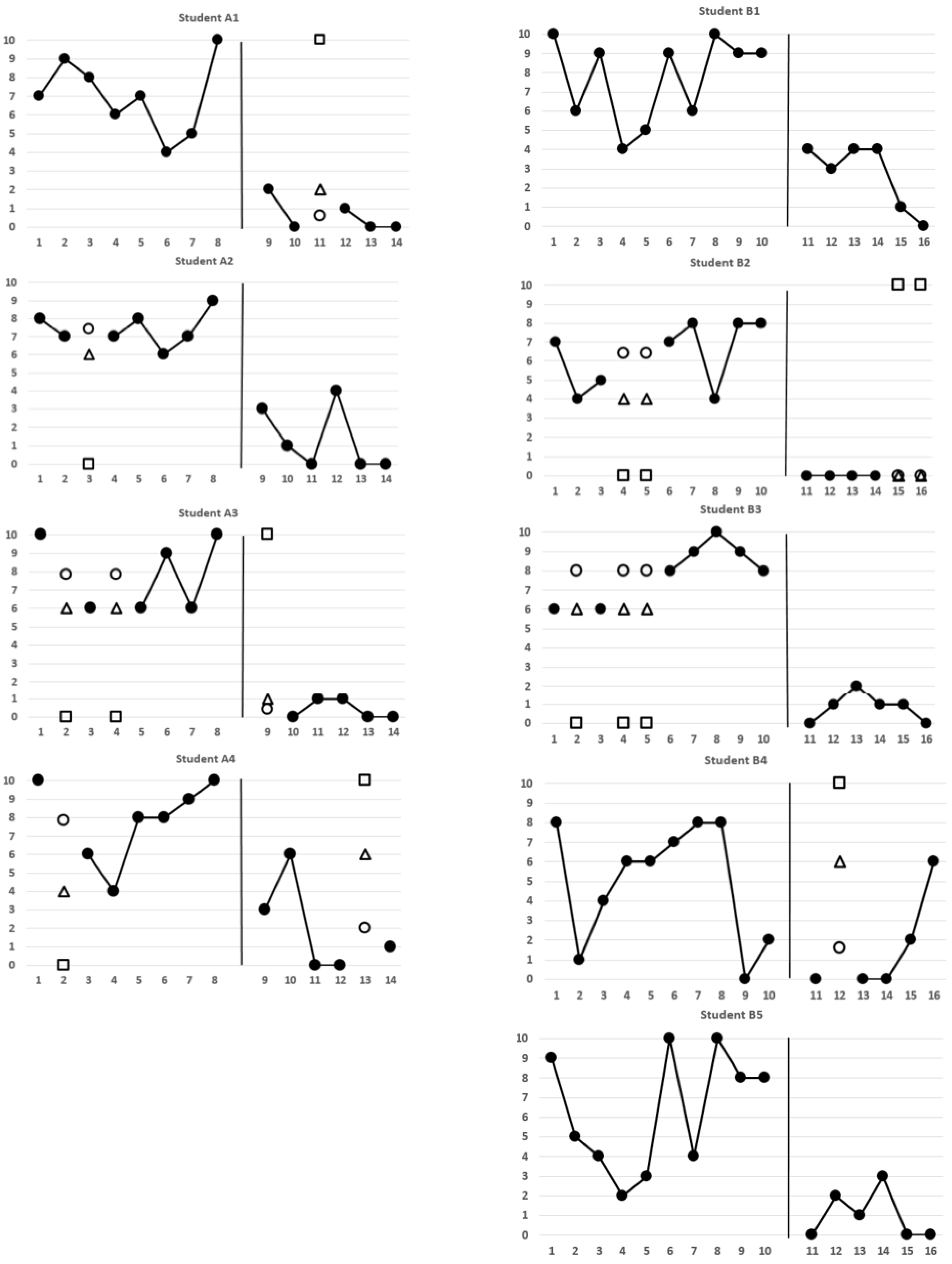
5.2. Student-Level Assessment Based on Level Change

A level change is the mean difference between two adjacent phases—one baseline and one intervention [25]. An effective RC should be indicated by a decrease in means from SSR1 to RC1 phases. To assess the level change for each student, we performed a one-tailed independent-samples t-test of mean decreases from SSR1 to RC1 under AD, MS, MM, and TMM methods (

Table 4. One-tailed independent-samples t-tests of SSR1 and RC1 means for all nine students under the available data (AD) method, and for Students A1–A4, and B2–B4 under mean substitution (MS), minimum-maximum (MM), and theoretical minimum-maximum (TMM) methods.

Method	AD
Student	MSSR12	MRC12	SDSSR1	SDRC1	t	df	P3
A1	7.00	0.60	2.00	0.89	6.67	11	<0.001
A2	7.43	1.33	0.98	1.75	7.92	11	<0.001
A3	7.83	0.40	2.04	0.55	7.85	9	<0.001
A4	7.86	2.00	2.19	2.55	4.27	10	0.001
B1 1	7.70	2.67	2.21	1.75	4.73	14	<0.001
B2	6.38	0.00	1.77	0.00	7.04	10	<0.001
B3	8.00	0.83	1.53	0.75	10.41	11	<0.001
B4	5.00	1.60	3.06	2.61	2.12	13	0.027
B5 1	6.30	1.00	3.02	1.26	4.05	14	0.001
	MS
A1	7.00	0.60	2.00	0.80	7.35	12	<0.001
A2	7.43	1.33	0.90	1.75	8.52	12	<0.001
A3	7.83	0.40	1.73	0.49	10.15	12	<0.001
A4	7.86	2.00	2.03	2.28	5.08	12	<0.001
B2	6.38	0.00	1.56	0.00	9.88	14	<0.001
B3	8.00	0.83	1.25	0.75	12.66	14	<0.001
B4	5.00	1.60	3.06	2.33	2.34	14	0.017
	MM
A1	7.00	0.83	2.00	0.98	6.90	12	<0.001
A2	7.25	1.33	1.04	1.75	7.94	12	<0.001
A3	7.38	0.50	1.92	0.55	8.43	12	<0.001
A4	7.38	2.67	2.45	2.80	3.35	12	0.003
B2	5.90	0.00	1.85	0.00	7.69	14	<0.001
B3	7.40	0.83	1.58	0.75	9.47	14	<0.001
B4	5.00	2.33	3.06	2.94	1.71	14	0.055
	TMM
A1	7.00	2.17	2.00	3.92	3.03	12	0.005
A2	6.50	1.33	2.78	1.75	3.98	12	0.001
A3	5.88	2.00	4.02	3.95	1.80	12	0.049
A4	6.88	3.33	3.44	3.98	1.78	12	<0.050
B2	5.10	3.33	3.11	5.16	0.86	14	0.202
B3	5.60	0.83	4.06	0.75	2.81	14	0.007
B4	5.00	3.00	3.06	4.15	1.11	14	0.143

¹ Had no missing scores during SSR1 and RC1; results were identical under all four methods. ² Bolded means are the smallest mean decreases under each method. ³ Shaded p values indicate non-significant results.

).

According to Table 4, all students’ level changes were in the desirable direction, namely, means decreased from SSR1 to RC1. Yet according to the significance level of the t-test, only Students A1 to A4, and B3 exhibited a significant mean decrease under all four methods. Student B2 exhibited a significant mean decrease under AD, MS, and MM, but not under TMM. Students B1 and B5 exhibited a significant mean decrease without missing data. Student B4 exhibited a significant mean decrease under AD and MS only. Furthermore, among the nine students, Student B4 yielded the smallest mean decrease under AD and MS (=5.00 − 1.60 = 3.40) and under MM (=5.00 − 2.33 = 2.67). Under TMM, Student B2 yielded the smallest mean decrease (=5.10 − 3.33 = 1.77) and Student B4 yielded the second smallest mean decrease (=5.00 − 3.00 = 2.00).

It is worth noting that phase means (i.e., M_SSR1 and M_RC1) under the MS method were identical to those under the AD method for Students A1 to A4 and B2 to B4; yet their phase SDs (i.e., SD_SSR1 or SD_RC1) were smaller under MS than under AD. The reduced phase SDs led to larger t-tests of phase mean differences under MS than under AD. A reduced phase variability is an inevitable consequence of applying the MS method.

5.3. Student-Level Assessment Based on Immediacy of the Effect

According to the WWC Standards Handbook, Version 4.0, “Immediacy of the effect refers to the change in level between the last three data points in one phase and the first three data points of the next.” [25]. The WWC Standards Handbook, Version 4.0 further states, “The more rapid (or immediate) the effect, the more convincing the inference that change in the outcome measure was due to manipulation of the independent variable” [25]. The assessment of immediacy of the effect is usually carried out by visual analysis, or by comparing the mean of the last three scores from one phase (i.e., SSR1) with the mean of the first three scores from the next phase (i.e., RC1) [25].

A visual analysis of Figure 1 seemed to suggest that all students, except for Student B4, exhibited an immediacy of the intervention effect. And means shown in

Table 5. One-tailed independent-samples t-tests of means from the last three scores of SSR1 to the first three scores of RC1 for all nine students under the available data (AD) method, and for Students A1, A3, and B4 under mean substitution (MS), minimum-maximum (MM), and theoretical minimum-maximum (TMM) methods.

	Three Scores 2		AD
Student	SSR1	RC1	MSSR13	MRC13	SDSSR1	SDRC1	t	df	P4
A1	4, 5, 10	2, 0, ?	6.33	1.00	3.21	1.41	2.13	3	0.062
A2 1	6, 7, 9	3, 1, 0	7.33	1.33	1.53	1.53	4.81	4	0.004
A3	9, 6, 10	?, 0, 1	8.33	0.50	2.08	0.71	4.91	3	0.008
A4 1	8, 9, 10	3, 6, 0	9.00	3.00	1.00	3.00	3.29	4	0.015
B1 1	10, 9, 9	4, 3, 4	9.33	3.67	0.58	0.58	12.02	4	<0.001
B2 1	4, 8, 8	0, 0, 0	6.67	0.00	2.31	0.00	5.00	4	0.004
B3 1	10, 9, 8	0, 1, 2	9.00	1.00	1.00	1.00	9.80	4	<0.001
B4	8, 0, 2	0, ?, 0	3.33	0.00	4.16	0.00	1.07	3	0.181
B5 1	10, 8, 8	0, 2, 1	8.67	1.00	1.15	1.00	8.69	4	<0.001
			MS
A1	4, 5, 10	2, 0, 0.6	6.33	0.87	3.21	1.03	2.81	4	0.024
A3	9, 6, 10	0.4, 0, 1	8.33	0.47	2.08	0.50	6.36	4	0.002
B4	8, 0, 2	0, 1.6, 0	3.33	0.53	4.16	0.92	1.14	4	0.160
			MM
A1	4, 5, 10	2, 0, 2	6.33	1.33	3.21	1.15	2.54	4	0.032
A3	9, 6, 10	1, 0, 1	8.33	0.67	2.08	0.58	6.15	4	0.002
B4	8, 0, 2	0, 6, 0	3.33	2.00	4.16	3.46	0.43	4	0.350
			TMM
A1	4, 5, 10	2, 0, 10	6.33	4.00	3.21	5.29	0.65	4	0.275
A3	9, 6, 10	10, 0, 1	8.33	3.67	2.08	5.51	1.37	4	0.121
B4	8, 0, 2	0, 10, 0	3.33	3.33	4.16	5.77	0.00	4	0.500

¹ Had no missing scores for the six sessions; results were identical under all four methods. ² Missing scores under AD were marked by “?”. ³ Bolded means are the smallest mean decreases under each method. ⁴ Shaded p values indicate non-significant results.

decreased from SSR1 to RC1 for all students. Yet according to one-tailed independent-samples t-tests of mean decreases, significant immediacy of the effect was demonstrated by six students (A2, A4, B1, B2, B3, and B5) who had no missing scores in the six sessions being analyzed. Two students (A1 and A3) partially demonstrated significant immediacy of the effect under two methods (MS and MM), and A3 additionally under the AD method. Student B4 did not demonstrate significant immediacy of the effect under any method. Furthermore, among the nine students, Student B4 yielded the smallest mean decreases under all methods (the mean decrease under AD = 3.33 − 0.00 = 3.33, under MS = 3.33 − 0.53 = 2.80, under MM = 3.33 − 2.00 = 1.33, and under TMM = 3.33 − 3.33 = 0.00). These findings suggested that immediacy of the RC effect was not fully demonstrated by Students A1, A3, and B4.

5.4. Student-Level Assessment Based on Nonoverlap

The WWC Standards Handbook, Version 4.0 defines overlap as “the proportion of data from one phase that overlaps with data from the previous phase” [25]. The WWC Standards Handbook, Version 4.0 further states, “the smaller the proportion of overlapping data points (or conversely, the larger the separation), the more compelling the demonstration of an effect.” [25]. We inferred from these statements that an intervention was assessed more directly by nonoverlap than by overlap between phases. Hence, Tarlow’s Tau was computed for each student as an index of nonoverlap [32,61]. The first step in computing Tarlow’s Tau is to test a baseline trend. If the trend is statistically significant, Tarlow’s Tau needs to be corrected for the trend. Chen, Wu, and Peng [32] referred to Tarlow’s baseline-trend-corrected Tau as Tau_c. If the baseline trend is tested not to be statistically significant, Tarlow’s Tau_noc is computed instead [32,61].

Both Tau_c and Tau_noc are Kendall’s Tau correlation coefficients ranging from −1 to +1 [62]. When all high scores are from the baseline phase and all low scores are from the intervention phase, Tau = −1. When all low scores are from the baseline phase and all high scores are from the intervention phase, Tau = +1. The larger the Tau_c or Tau_noc in absolute value, the more nonoverlap between baseline and intervention scores. Tau_c and Tau_noc are tested using a normal approximate test, when the combined baseline and intervention scores are numbered 10 or more [62]. All nine students had 10 or more scores from the combined SSR1 and RC1 phases. The computation and statistical test of Tau_c and Tau_noc were facilitated by Baseline Corrected Tau Calculator at http://ktarlow.com/stats/tau/ [59].

For eight students, excluding B3, the baseline trend was insignificant under all four methods. Hence, Tau_noc was computed and tested for them. For Student B3 under MS and MM, Tau_c was computed and tested because of a significant baseline trend. For Student B3 under AD and TMM, Tau_noc was computed and tested because of an insignificant baseline trend. Results are presented in

Table 6. One-tailed Tarlow’s Tau for all nine students under available data (AD), mean substitution (MS), minimum-maximum (MM), and theoretical minimum-maximum (TMM) methods. SE is standard error. Tau_noc was computed except for Student B3 under MS and MM.

	AD			MS			MM			TMM
Student	Tau	SE	p	Tau	SE	p	Tau	SE	p	Tau	SE	P4
A1	−0.735	0.266	0.002	−0.743	0.253	0.001	−0.747	0.251	0.001	−0.514	0.324	0.019
A2	−0.769	0.251	0.002	−0.756	0.247	0.001	−0.760	0.245	0.001	−0.625	0.295	0.007
A3	−0.799	0.256	0.004	−0.765	0.243	0.001	−0.805	0.224	0.001	−0.336	0.356	0.103
A4	−0.687	0.297	0.006	−0.696	0.271	0.002	−0.598	0.303	0.008	−0.364	0.352	0.076
B1 1	−0.715	0.247	0.001	(same as AD results)
B2	−0.763	0.264	0.004	−0.778	0.222	<0.001	−0.795	0.215	<0.001	−0.156	0.349	0.269
B3 2	−0.769	0.251	0.002	−0.710 2	0.249	<0.001 3	−0.713 2	0.248	<0.001 3	−0.380	0.327	0.055
B4	−0.472	0.322	0.027	−0.474	0.311	0.021	−0.405	0.323	0.044	−0.275	0.340	0.124
B5 1	−0.683	0.258	0.002	(same as AD results)

¹ Had no missing scores; results were identical under all four methods. ² Tau_c was computed because of a significant baseline trend (p ≤ 0.03, 2-tailed); the statistical test of the baseline trend can be low-powered if baseline scores are fewer than seven [61]. ³ Tau_c was significant at p = 0.0007 after adjusting out-of-range predicted scores using the Tauc R function at https://osf.io/h75fd/?view_only=0c40cd0678ed45798501de418cca0f44 [32]. ⁴ Shaded ps indicate non-significant results.

.

All Taus in Table 6 were in the desirable direction, namely, most high scores were from SSR1 and most low scores were from RC1. Yet according to the one-tailed standard normal test, only two students (A1 and A2) demonstrated significant nonoverlap between SSR1 and RC1 under all methods. Two students (B1 and B5) demonstrated significant nonoverlap without missing scores. Five students (A3, A4, B2, B3, and B4) demonstrated significant nonoverlap under AD, MS, and MM methods, but not under the TMM method.

5.5. Conclusions Based on Four Assessments

Class-level assessment presented in Section 5.1 led us to conclude that the RC intervention was effective in decreasing the intervals with disruptive behaviors from SSR1 to RC1 phases for Class A and Class B separately and as one group. This conclusion was supported by magnitudes of the g effect size index, and by significant tests of the gs.

Student-level assessments presented in Section 5.2 to 5.4 led us to conclude that the RC intervention was not equally effective for all students. The RC intervention was effective for Students A2, B1, B5, and ineffective for Student B4. The effectiveness of the RC intervention was inconclusive with Students A1, A3, A4, B2, and B3. We reached these conclusions on the basis of three separate assessments: level change, immediacy of the effect, and nonoverlap. Student A2 demonstrated the RC effect on all three assessments with missing scores imputed by all four methods. Students B1 and B5 did so without any missing score. Student B4 did not demonstrate the RC effect on any of the three assessments using any of the four methods to impute missing scores. The remaining students (A1, A3, A4, B2, and B3) demonstrated the RC effect on one or two assessments with missing scores imputed by all methods. The detailed analyses of the RC effect on individual students expanded and enriched conclusions reported in Lambert et al. [34].

6. Discussion and Conclusions

Missing data is a rule rather than an exception in group designs as well as in SCD studies [18,48]. The average missing data rate uncovered in our review of 428 SCD articles was 21%. And a 20% of missing data was benchmarked by literature on studies related to youth, school-based programs, and clinical research [13,14,15]. Given the substantial presence of missing data in SCD studies and potential consequences of treating them inadequately [16,18,22], it is imperative that researchers and practitioners be informed of strategies to deal with missing data properly.

The SCRIBE 2016 provides a guide on why and how missing data should be reported in order to support claims made about intervention effects. However, the SCRIBE 2016 or the WWC handbooks [24,25,26,27] offer no recommendation for viable missing data methods. To fill this void, this paper reviews nine missing data methods including: the available data method, six single imputation methods, and two model-based methods. Their implementations, strengths, weaknesses, assumptions, and applications are discussed and summarized in Section 4. The available data method and three single imputation methods, namely, MS, MM, and TMM, were additionally demonstrated in assessing an intervention effect in published data (Section 5). Assessment results, along with visual analysis of data, were interpreted for classes in terms of an effect size index and for participants in terms of level change, immediacy of the effect, and nonoverlap. Differences in results were noted among the four methods. To assist readers with making informed decisions about treating missing data in SCD studies, we discuss contingencies for implementing missing data methods in Section 6.1 and strategies for managing missing data in Section 6.2 below.

6.1. Contingencies for Implementing Missing Data Methods

The proportion of missing scores per participant is one key factor in determining the quality of visual and statistical inferences. The literature has not established an acceptable proportion for valid visual and statistical inferences [11,23]. For statistical inferences based on group designs, Schafer [47] considered 5% or less to be inconsequential. Bennett [63] asserted that 10% or greater is likely to bias statistical analysis. For SCD studies, McDonald et al. [46] suggested that single imputation methods be employed, given 10% or less missing scores. McDonald et al. [46] further suggested that a missing score be substituted by the mean or median of three preceding and three subsequent scores, namely, the AMS method discussed in Section 4 and summarized in Table 1. Because AMS was inapplicable to the Lambert data, we proposed the MM and the TMM methods as alternative strategies to deal with 12.5% missing scores in Class A and 10% in Class B (Section 5). The relative merits of these two methods are extensively discussed in Section 4 and summarized in Table 1.

Missing data mechanism is another key factor that impacts statistical results [64]. All missing data methods described in Section 4, except for the AD method, yield valid statistical inferences under MAR. The AD method requires the stronger MCAR condition to yield valid statistical inferences. The tenability of MCAR may be examined using Little’s multivariate test [65]. Yet, the test result does not prove that MCAR holds [21,23,38,47]. Likewise, it is impossible to test whether the MAR condition holds, given only the observed data [66,67,68]. The MAR assumption can be made more plausible if auxiliary variables that could account for missingness are included in the statistical inferential process. Thus, the literature on missing data methods often suggests including additional variables into a statistical model in order to make the missing data mechanism ignorable or MAR [60,69,70,71]. Such a suggestion is applicable to model-based methods, namely, MI and EM.

Indeed, MI and EM promise to handle missing scores efficiently in statistical analyses of SCD data, if (a) data meet the multivariate normality assumption, (b) the model for the observed and the missing scores is correct under MAR, (c) correlations among scores are mild, and (d) the algorithm converges. The adequacy of a model specified for MI or EM directly impacts the quality of estimates (e.g., means, SDs, imputed scores) derived from the model [18,31,55]. It is a daunting task to specify a correct model so as to trust MI or EM results. Furthermore, MI’s algorithm may not converge, especially when the proportion of missing data is high and data are not missing at random, because MI imputes each missing score multiple times [18,21,51,72]. MI or EM has not been shown in published studies to complement visual analysis results. Both methods are concerned with estimating population parameters efficiently and accurately, but not individual scores. The notion of a population or its parameter is less clearly delineated in SCDs than in group designs. Perhaps for these reasons, MI or EM has not been regularly applied in SCD contexts to deal with missing scores [6].

In order for MI or EM to be successfully and widely applied in a variety of SCD studies, researchers and practitioners need to be aware of issues (a) to (d) outlined in the previous paragraph. Additional research is needed to elucidate their properties (e.g., robustness of assumptions, Type I error control, statistical power) under different missing data rates and data characteristics (e.g., non-normally distributed scores). Similar research is also needed for the six single imputation methods discussed in this paper, even though MS, LOCF, and LIN with or without a noise have been applied in published studies more often than AMS, MM, or TMM. In Section 6.2 below, we offer several strategies for managing missing data practically according to the SCRIBE 2016 and the literature on missing data methods.

6.2. Strategies for Managing Missing Data

First, minimize missing scores as much as possible. Protocols for implementation of an intervention, data collection, and data entry should be thoroughly tested and strictly followed to avoid causes of missing information. For example, if participants’ behaviors are to be observed in a study, the observer needs to make sure that she/he can observe participants clearly from all angles and nothing blocks the view during the entire observation period. Or, if needed, recruit and train sufficient observers to prevent a planned session from canceling due to an observer’s absence.

Second, when missing data occurred, acknowledge them and report reasons and techniques for dealing with them [19]. For approximately 43% of articles we reviewed, there was no acknowledgement of missing data; yet data graphs clearly revealed the presence of missing data. Researchers and interventionists are encouraged to make a concerted effort to improve the reporting of missing data in SCD studies.

Third, to select a strategy to properly treat missing data in a SCD context, one needs to consider the proportion of missing data, the missing data mechanism, and the implementation of a missing data method [18,23]. If the proportion of missing data is more than 50%, one should carefully investigate why this happens before deciding if additional data need to be collected. If MCAR can be assumed or the proportion of missing data is less than 5%, the AD method is a viable strategy. If MAR can be assumed, the proportion of missing data is moderate, say, between 5% and 30%, and a conservative assessment of an intervention is desired, MM or TMM can be used in conjunction with visual analysis of data. If a less-than-conservative assessment of an intervention is desired under MAR and the missing rate is moderate, AMS or LIN can be used in conjunction with visual analysis of data. If MAR can be assumed, the missing rate is moderate, and estimating population parameters is desired, either MI or EM may be used as a strategy. If randomization is used in designing a study and also in assessing an intervention effect using a randomization test, the randomized marker method may be used to treat missing data (see Appendix A). Researchers and practitioners can employ multiple methods to ascertain consistency among results, as it was demonstrated in Section 5.

Missing information in SCD contexts does occur frequently. It is hoped that the extensive discussion of problems caused by missing scores and their possible treatments empower researchers and practitioners to account for missing scores effectively and to support evidence-based claims vigorously in single-case intervention studies.

References

1. Harrison, J.R.; Soares, D.A.; Rudzinski, S.; Johnson, R. Attention Deficit Hyperactivity Disorders and Classroom-Based Interventions: Evidence-Based Status, Effectiveness, and Moderators of Effects in Single-Case Design Research. Rev. Educ. Res. 2019, 89, 569–611. [Google Scholar] [CrossRef]
2. Long, A.C.J.; Miller, F.G.; Upright, J.J. Classroom management for ethnic–racial minority students: A meta-analysis of single-case design studies. Sch. Psychol. 2019, 34, 1–13. [Google Scholar] [CrossRef]
3. Martinez, J.R.; Waters, C.L.; Conroy, M.A.; Reichow, B. Peer-Mediated Interventions to Address Social Competence Needs of Young Children With ASD: Systematic Review of Single-Case Research Design Studies. Top. Early Child. Spéc. Educ. 2021, 40, 217–228. [Google Scholar] [CrossRef]
4. Ratanavivan, W.; Ricard, R.J. Effects of a Motivational Interviewing-Based Counseling Program on Classroom Behavior of Children in a Disciplinary Alternative Education Program. J. Couns. Dev. 2018, 96, 410–423. [Google Scholar] [CrossRef]
5. Perrin, C.J.; Miller, N.; Haberlin, A.T.; Ivy, J.W.; Meindl, J.N.; Neef, N.A. MEASURING AND REDUCING COLLEGE STUDENTS’ PROCRASTINATION. J. Appl. Behav. Anal. 2011, 44, 463–474. [Google Scholar] [CrossRef] [PubMed] [Green Version]
6. McDonald, S.; Quinn, F.; Vieira, R.; O’Brien, N.; White, M.; Johnston, D.W.; Sniehotta, F.F. The state of the art and future opportunities for using longitudinal n-of-1 methods in health behaviour research: A systematic literature overview. Health Psychol. Rev. 2017, 11, 307–323. [Google Scholar] [CrossRef]
7. Horner, R.H.; Carr, E.G.; Halle, J.W.; McGee, G.G.; Odom, S.L.; Wolery, M. The Use of Single-Subject Research to Identify Evidence-Based Practice in Special Education. Except. Child. 2005, 71, 165–179. [Google Scholar] [CrossRef]
8. Kazdin, A.E. Single-case experimental designs. Evaluating interventions in research and clinical practice. Behav. Res. Ther. 2019, 117, 3–17. [Google Scholar] [CrossRef]
9. Radley, K.C.; Dart, E.H.; Fischer, A.J.; Collins, T.A. Publication trends for single-case methodology in school psychology: A systematic review. Psychol. Sch. 2020, 57, 683–698. [Google Scholar] [CrossRef]
10. Shadish, W.R.; Sullivan, K.J. Characteristics of single-case designs used to assess intervention effects in 2008. Behav. Res. Methods 2011, 43, 971–980. [Google Scholar] [CrossRef] [Green Version]
11. Smith, J.D. Single-case experimental designs: A systematic review of published research and current standards. Psychol. Methods 2012, 17, 510–550. [Google Scholar] [CrossRef] [PubMed] [Green Version]
12. Allison, D.B.; Silverstein, J.M.; Gorman, B.S. Power, sample size estimation, and early stopping rules. In Design and Analysis of Single-Case Research; Franklin, R.D., Allison, D.B., Gorman, B.S., Eds.; Lawrence Erlbaum Associates: Mahwah, NJ, USA, 1996; pp. 335–371. [Google Scholar]
13. Hall, J.A.; US Department of Health and Human Services; National Institute on Drug Abuse Skills Training for Pregnant and Parenting Adolescents. PsycEXTRA Dataset 1995, 156, 255–290. [CrossRef]
14. Kellam, S.G.; Rebok, G.W.; Ialongo, N.; Mayer, L.S. The Course and Malleability of Aggressive Behavior from Early First Grade into Middle School: Results of a Developmental Epidemiologically-based Preventive Trial. J. Child Psychol. Psychiatry 1994, 35, 259–281. [Google Scholar] [CrossRef] [PubMed]
15. Mason, M.J. A Review of Procedural and Statistical Methods for Handling Attrition and Missing Data in Clinical Research. Meas. Evaluation Couns. Dev. 1999, 32, 111–118. [Google Scholar] [CrossRef]
16. Chen, L.-T.; Peng, C.-Y.J.; Chen, M.-E. Computing Tools for Implementing Standards for Single-Case Designs. Behav. Modif. 2015, 39, 835–869. [Google Scholar] [CrossRef]
17. Chiu, M.M.; Roberts, C.A. Improved analyses of single cases: Dynamic multilevel analysis. Dev. Neurorehabilit. 2016, 21, 253–265. [Google Scholar] [CrossRef]
18. Peng, C.-Y.J.; Chen, L.-T. Handling missing data in single-case studies. J. Mod. Appl. Stat. Methods 2018, 17, 5. [Google Scholar] [CrossRef] [Green Version]
19. Tate, R.L.; Perdices, M.; Rosenkoetter, U.; McDonald, S.; Togher, L.; Shadish, W.; Horner, R.; Kratochwill, T.; Barlow, D.H.; Kazdin, A.; et al. The Single-Case Reporting Guideline In BEhavioural Interventions (SCRIBE) 2016: Explanation and Elaboration. Arch. Sci. Psychol. 2016, 4, 10–31. [Google Scholar] [CrossRef] [Green Version]
20. Rubin, D.B. Multiple Imputation for Nonresponse in Surveys; Wiley & Sons: New York, NY, USA, 1987. [Google Scholar]
21. Gadbury, G.; Schafer, J.L. Analysis of Incomplete Multivariate Data (Monographs on Statistics and Applied Probability, No. 72). J. Am. Stat. Assoc. 2000, 95, 1013. [Google Scholar] [CrossRef]
22. Shadish, W.R.; Cook, T.D.; Campbell, D.T. Experimental and Quasi-Experimental Designs for Generalized Causal Inference, 2nd ed.; Houghton Mifflin: Boston, MS, USA, 2002. [Google Scholar]
23. Dong, Y.; Peng, C.-Y.J. Principled missing data methods for researchers. SpringerPlus 2013, 2, 1–17. [Google Scholar] [CrossRef] [Green Version]
24. What Works Clearinghouse. WWC Procedures Handbook; Version 4.0; 2017. Available online: https://ies.ed.gov/ncee/wwc/Docs/referenceresources/wwc_procedures_handbook_v4.pdf (accessed on 1 October 2020).
25. What Works Clearinghouse. WWC Standards Handbook; Version 4.0; 2017. Available online: https://ies.ed.gov/ncee/wwc/Docs/referenceresources/wwc_standards_handbook_v4.pdf (accessed on 1 October 2020).
26. What Works Clearinghouse. WWC Procedures Handbook; Version 4.1; 2020. Available online: https://ies.ed.gov/ncee/wwc/Docs/referenceresources/WWC-Procedures-Handbook-v4-1-508.pdf (accessed on 1 October 2020).
27. What Works Clearinghouse. WWC Standards Handbook; Version 4.1; 2020. Available online: https://ies.ed.gov/ncee/wwc/Docs/referenceresources/WWC-Standards-Handbook-v4-1-508.pdf (accessed on 1 October 2020).
28. Goodwin, L.D.; Goodwin, W.L. Statistical Techniques in AERJ Articles, 1979–1983: The Preparation of Graduate Students to Read the Educational Research Literature. Educ. Res. 1985, 14, 5–11. [Google Scholar] [CrossRef]
29. Dworkin, R.J. Hidden Bias in the Use of Archival Data. Evaluation Heal. Prof. 1987, 10, 173–185. [Google Scholar] [CrossRef]
30. Reichow, B.; Barton, E.E.; Maggin, D.M. Development and applications of the single-case design risk of bias tool for evaluating single-case design research study reports. Res. Dev. Disabil. 2018, 79, 53–64. [Google Scholar] [CrossRef] [PubMed]
31. Chen, L.-T.; Feng, Y.; Wu, P.-J.; Peng, C.-Y.J. Dealing with missing data by EM in single-case studies. Behav. Res. Methods 2020, 52, 131–150. [Google Scholar] [CrossRef] [PubMed] [Green Version]
32. Chen, L.-T.; Wu, P.-J.; Peng, C.-Y.J. Accounting for baseline trends in intervention studies: Methods, effect sizes, and software. Cogent Psychol. 2019, 6. [Google Scholar] [CrossRef]
33. Cosbey, J.; Muldoon, D. EAT-UP™ Family-Centered Feeding Intervention to Promote Food Acceptance and Decrease Challenging Behaviors: A Single-Case Experimental Design Replicated Across Three Families of Children with Autism Spectrum Disorder. J. Autism Dev. Disord. 2017, 47, 564–578. [Google Scholar] [CrossRef] [PubMed]
34. Lambert, M.C.; Cartledge, G.; Heward, W.L.; Lo, Y.-Y. Effects of Response Cards on Disruptive Behavior and Academic Responding During Math Lessons by Fourth-Grade Urban Students. J. Posit. Behav. Interv. 2006, 8, 88–99. [Google Scholar] [CrossRef]
35. Stiegler, J.R.; Molde, H.; Schanche, E. Does an emotion-focused two-chair dialogue add to the therapeutic effect of the empathic attunement to affect? Clin. Psychol. Psychother. 2018, 25, e86–e95. [Google Scholar] [CrossRef]
36. Matta, M.; Volpe, R.J.; Briesch, A.M.; Owens, J.S. Five direct behavior rating multi-item scales: Sensitivity to the effects of classroom interventions. J. Sch. Psychol. 2020, 81, 28–46. [Google Scholar] [CrossRef]
37. Smith, J.D.; Eichler, W.C.; Norman, K.R.; Smith, S.R. The Effectiveness of Collaborative/Therapeutic Assessment for Psychotherapy Consultation: A Pragmatic Replicated Single-Case Study. J. Pers. Assess. 2014, 97, 261–270. [Google Scholar] [CrossRef]
38. Little, R.J.A.; Rubin, D.B. Statistical Analysis with Missing Data, 2nd ed.; John Wiley & Sons, Inc.: New Jersey, NJ, USA, 2002. [Google Scholar]
39. Borckardt, J.J.; Nash, M.R. Simulation modelling analysis for small sets of single-subject data collected over time. Neuropsychol. Rehabilitation 2014, 24, 492–506. [Google Scholar] [CrossRef]
40. Busk, P.L.; Marascuilo, L.A. Autocorrelation in single-subject research: A counterargument to the myth of no autocorrelation. Behav. Assess. 1988, 10, 229–242. [Google Scholar]
41. Huitema, B.E.; Mckean, J.W. Design Specification Issues in Time-Series Intervention Models. Educ. Psychol. Meas. 2000, 60, 38–58. [Google Scholar] [CrossRef]
42. Shadish, W.R.; Hedges, L.V.; Pustejovsky, J.E. Analysis and meta-analysis of single-case designs with a standardized mean difference statistic: A primer and applications. J. Sch. Psychol. 2014, 52, 123–147. [Google Scholar] [CrossRef] [PubMed]
43. Rafii, M.S.; Baumann, T.L.; Bakay, R.A.E.; Ostrove, J.M.; Siffert, J.; Fleisher, A.S.; Herzog, C.D.; Barba, D.; Pay, M.; Salmon, D.P.; et al. A phase1 study of stereotactic gene delivery of AAV2-NGF for Alzheimer’s disease. Alzheimer’s Dement. 2014, 10, 571–581. [Google Scholar] [CrossRef]
44. Daza, E.J. Causal Analysis of Self-tracked Time Series Data Using a Counterfactual Framework for N-of-1 Trials. Methods Inf. Med. 2018, 57, e10–e21. [Google Scholar] [CrossRef] [Green Version]
45. Pole, N.; Ablon, J.S.; O’Connor, L.E. Using psychodynamic, cognitive behavioral, and control mastery prototypes to predict change: A new look at an old paradigm for long-term single-case research. J. Couns. Psychol. 2008, 55, 221–232. [Google Scholar] [CrossRef] [Green Version]
46. McDonald, S.; Vieira, R.; Johnston, D.W. Analysing N-of-1 observational data in health psychology and behavioural medicine: A 10-step SPSS tutorial for beginners. Heal. Psychol. Behav. Med. 2020, 8, 32–54. [Google Scholar] [CrossRef] [Green Version]
47. Schafer, J.L. Multiple imputation: A primer. Stat. Methods Med. Res. 1999, 8, 3–15. [Google Scholar] [CrossRef] [PubMed]
48. Peng, C.-Y.J.; Harwell, M.R.; Liou, S.-M.; Ehman, L.H. Advances in missing data methods and implications for educational research. In Real Data Analysis; Sawilowsky, S.S., Ed.; Information Age Pub: New York, NY, USA, 2006; pp. 31–78. [Google Scholar]
49. Hobbs, N.; Dixon, D.; Johnston, M.; Howie, K. Can the theory of planned behaviour predict the physical activity behaviour of individuals? Psychol. Heal. 2013, 28, 234–249. [Google Scholar] [CrossRef] [PubMed]
50. Nyman, S.R.; Goodwin, K.; Kwasnicka, D.; Callaway, A. Increasing walking among older people: A test of behaviour change techniques using factorial randomised N-of-1 trials. Psychol. Health 2016, 31, 313–330. [Google Scholar] [CrossRef] [PubMed] [Green Version]
51. Quinn, F.; Johnston, M.; Johnston, D.W. Testing an integrated behavioural and biomedical model of disability in N-of-1 studies with chronic pain. Psychol. Health 2013, 28, 1391–1406. [Google Scholar] [CrossRef]
52. Dempster, A.P.; Laird, N.M.; Rubin, D.B. Maximum Likelihood from Incomplete Data Via the EM Algorithm. J. R. Stat. Soc. Ser. B (Stat. Methodol.) 1977, 39, 1–22. [Google Scholar] [CrossRef]
53. Rubin, D.B. Inference and missing data. Biometrika 1976, 63, 581–592. [Google Scholar] [CrossRef]
54. Graham, J.W. Adding Missing-Data-Relevant Variables to FIML-Based Structural Equation Models. Struct. Equ. Model. A Multidiscip. J. 2003, 10, 80–100. [Google Scholar] [CrossRef]
55. Smith, J.D.; Borckardt, J.J.; Nash, M.R. Inferential Precision in Single-Case Time-Series Data Streams: How Well Does the EM Procedure Perform When Missing Observations Occur in Autocorrelated Data? Behav. Ther. 2012, 43, 679–685. [Google Scholar] [CrossRef] [PubMed] [Green Version]
56. Buu, A. Analysis of Longitudinal Data with Missing Values: A Methodological Comparison. Ph.D. Thesis, Indiana University, Bloomington, IN, USA, 1999. [Google Scholar]
57. Horner, R.H.; Swaminathan, H.; Sugai, G.; Smolkowski, K. Considerations for the Systematic Analysis and Use of Single-Case Research. Educ. Treat. Child. 2012, 35, 269–290. [Google Scholar] [CrossRef]
58. Marson, D.; Shadish, W.R. User guide for DHPS, D_Power, and GPHDPwr SPSS macros, Version 1.0. 2014.
59. Tarlow, K.R. Baseline Corrected Tau Calculator. Available online: http://www.ktarlow.com/stats/tau (accessed on 1 October 2020).
60. Hedges, L.V.; Pustejovsky, J.E.; Shadish, W.R. A standardized mean difference effect size for single case designs. Res. Synth. Methods 2012, 3, 224–239. [Google Scholar] [CrossRef] [PubMed]
61. Tarlow, K.R. An Improved Rank Correlation Effect Size Statistic for Single-Case Designs: Baseline Corrected Tau. Behav. Modif. 2016, 41, 427–467. [Google Scholar] [CrossRef] [PubMed]
62. Kendall, M. Rank Correlation Methods, 3rd ed.; Hafner Publishing Company: New York, NY, USA, 1962. [Google Scholar]
63. Bennett, D.A. How can I deal with missing data in my study? Aust. N. Z. J. Public Heal. 2001, 25, 464–469. [Google Scholar] [CrossRef]
64. Tabachnick, B.G.; Fidell, L.S. Using Multivariate Statistics, 6th ed.; Allyn & Bacon: Boston, MS, USA, 2012. [Google Scholar]
65. Little, R.J.A.; Schenker, N. Missing data. In Handbook of Statistical Modeling for the Social and Behavioral Sciences; Arminger, G., Clogg, C.C., Sobel, M.E., Eds.; Plenum Press: New York, NY, USA, 1995; pp. 39–75. [Google Scholar]
66. Carpenter, J.R.; Goldstein, H. Multiple imputation in MLwiN. Multilevel Model. Newsl. 2004, 16, 9–18. [Google Scholar]
67. Horton, N.J.; Kleinman, K.P. Much Ado About Nothing. Am. Stat. 2007, 61, 79–90. [Google Scholar] [CrossRef] [PubMed]
68. White, I.R.; Royston, P.; Wood, A.M. Multiple imputation using chained equations: Issues and guidance for practice. Stat. Med. 2010, 30, 377–399. [Google Scholar] [CrossRef] [PubMed]
69. Allison, P.D. Missing Data; Sage Publications: Thousand Oaks, CL, USA, 2001. [Google Scholar]
70. Collins, L.M.; Schafer, J.L.; Kam, C.-M. A comparison of inclusive and restrictive strategies in modern missing data procedures. Psychol. Methods 2001, 6, 330–351. [Google Scholar] [CrossRef]
71. Rubin, D.B. Multiple Imputation after 18+ Years. J. Am. Stat. Assoc. 1996, 91, 473–489. [Google Scholar] [CrossRef]
72. Schomaker, M.; Heumann, C. Bootstrap inference when using multiple imputation. Stat. Med. 2018, 37, 2252–2266. [Google Scholar] [CrossRef]
73. Edgington, E.; Onghena, P. Randomization Tests; CRC Press: Boca Raton, FL, USA, 2007. [Google Scholar]
74. Bulté, I.; Onghena, P. An R package for single-case randomization tests. Behav. Res. Methods 2008, 40, 467–478. [Google Scholar] [CrossRef] [Green Version]
75. De, T.K.; Michiels, B.; Tanious, R.; Onghena, P. Handling missing data in randomization tests for single-case experiments: A simulation study. Behav. Res. Methods 2020, 52, 1355–1370. [Google Scholar] [CrossRef]
Figure 1. Number of intervals with disruptive behaviors of nine students during SSR1 (first single student response, or baseline) and RC1 (first response cards, or intervention) phases. Solid dots (●) represent observed scores in Lambert et al. (2006). Breaks indicate missing scores. Hollow circles (○) represent imputed scores from the mean substitution (MS) method, triangles (∆) represent imputed scores from the minimum-maximum (MM) method, and squares (□) represent imputed scores from the theoretical minimum-maximum (TMM) method.
Education 11 00076 g001