Article

Dynamics of Macroeconomic Uncertainty on Economic Growth in the Presence of Fiscal Consolidation in South Africa from 1994 to 2022

by
Eugene Msizi Buthelezi
Department of Economics, University of Free State, Bloemfontein 9301, South Africa
Economies 2023, 11(4), 119; https://doi.org/10.3390/economies11040119
Submission received: 12 January 2023 / Revised: 20 February 2023 / Accepted: 20 February 2023 / Published: 15 April 2023
(This article belongs to the Section Macroeconomics, Monetary Economics, and Financial Markets)

Abstract

:
This paper investigates the effects of macroeconomic uncertainty on economic growth in the presence of fiscal consolidation in South Africa. Markov-switching dynamic regression (MSDR) and time-varying parameter vector autoregression (TVP-VAR) were performed using time series data from 1994 to 2022. Less attention has been given directly to the investigation of macroeconomic uncertainty in different regimes of economic growth in South Africa. Three states are found for economic growth, with mean growth rates of negative 6.29% and positive 3.90% and 1.47%, respectively. Macroeconomic uncertainty was found to have a negative impact of 6.72%, 4.38%, and 3.08% in states 1 to 3, respectively. Fiscal consolidation provided an accommodative policy, as it reduced the negative impact of macroeconomic uncertainty by 3.17%, 1.80%, and 0.92% in states 1 to 3, respectively. However, fiscal consolidation does not completely reduce the negative impact of macroeconomic uncertainty. The transition probabilities of economic growth moving and returning to the same states are 29.46%, 34.07%, and 58.02%, in each state, respectively. The time-varying impulse response functions showed that the shock of macroeconomic uncertainty harms economic growth. Nevertheless, the multiplier effect is not large; however, the economy operates below equilibrium and does not restore equilibrium after the effect of macroeconomic uncertainty. This reflects that it takes time for macroeconomic uncertainty to filter out of the South African economy. It is recommended that fiscal consolidation be considered as an accommodative fiscal policy to reduce macroeconomic uncertainty but not as a main policy for economic growth.

1. Background

There is growing interest among scholars in investigating the impact of macroeconomic uncertainty on economic growth, which includes the following investigations: Mandeya and Ho (2021), and Balcilar et al. (2022), among others. However, no consensus has been reached as to the impact of macroeconomic uncertainty on economic growth, as both positive and negative results are found (Mumtaz and Theodoridis (2018), Gupta and Jooste (2018), Redl (2018), Olanipekun et al. (2019), Mandeya and Ho (2021), and Balcilar et al. (2022). Macroeconomic uncertainty refers to a lack of knowledge about the set of possible effects and their related probabilities because the final results are highly particular or complex, which makes forecasting difficult (Bloom 2014). One of the broad measures of macroeconomic uncertainty is the world uncertainty for the South Africa index (WUI). Less attention has been given directly to the investigation of macroeconomic uncertainty in different regimes of economic growth in the presence of fiscal consolidation in South Africa. The main contribution of this paper to fill that gap. The thinking around fiscal consolidation is that government expenditure cuts and tax increases will result in a fall in debt because present, forwards-looking economic agents will anticipate a reduction in tax and interest rates. This will increase permeant income as well crowed-in investment; as such, there will be an increase in economic activities, leading to higher economic growth and higher tax collection that can be used to reduce government debt (Alesina and Ardagna 2010; Mankiw 2019). One of the broad measures of discretionary government intervention to reduce the government debt that defines fiscal consolidation episodes is the cyclically adjusted primary balance (CAPB). The measure is concerned with the identification of discretionary fiscal policy changes in tax and government expenditure by filtering out changes that are due to economic fluctuations in tax as well as government expenditure (Alesina et al. 2019). The investigation of aggregate effects of global uncertainty with evidence from an emerging economy including South Africa was undertaken by Ahiadorme (2022) using vector autoregressions (VARs). It was discovered that shocks related to global unpredictability are a significant cause of economic fluctuations. Additionally, the predicted macroeconomic uncertainty harms the financial and stock markets and significantly explains the cyclical downturn in economic growth.
In 2014, the Financial and Fiscal Commission (FFC) in South Africa recommended more fiscal consolidation stances to restore the fiscal position to increase economic growth and reduce government debt (BR 2014). The FFC recommendation outlined that “Fiscal consolidation can no longer be postponed. Ensuring continued progress towards a better life obliges the government to safeguard public finances by acting within fiscal limits that can be sustained over the long term. To do otherwise would risk exposing the country to a debt trap, with damaging consequences for development for many years to come” (MTBPS 2014). The Fiscal Responsibility Bill (FRB) was tabled for discussion in the parliament of SA in 2018. The bill seeks to introduce government expenditure cuts, limit new government borrowing, maintain an expenditure ceiling, and eliminate wasteful expenditure (FRB 2018). In 2019, the International Monterey Fund (IMF), Standard and Poor’s, Moody’s, and Fitch stressed that SA needs to implement a credible fiscal strategy and fiscal consolidation to contain the rise in government debt. This recommendation came with concern that the country is faced with high government debt and that there is policy uncertainty (IMF 2020).
Despite this effort, the economic growth is at the mean rate of 2.43%, which is below the 5% stipulated in the South African macroeconomic policy of the National Development Plan in 2013 (National Planning Commission 2013). It is against this background that it is critical to investigate the dynamics of macroeconomic uncertainty in different regimes of economic growth in the presence of fiscal consolidation in South Africa. The key questions of this paper are as follows: What is the impact of macroeconomic uncertainty in different regimes of economic growth in the presence of fiscal consolidation in South Africa? How long will economic growth be at a higher rate and a lower rate? What is the probability of transitioning to different regimes of economic growth in the presence of fiscal consolidation and macroeconomic uncertainty? What is the impact of macroeconomic uncertainty and fiscal consolidation shocks? Given the questions of this paper, the hypotheses are as follows:
Null:Macroeconomic uncertainty has no impact on different regimes of economic growth in the presence of fiscal consolidation.
Alt:Macroeconomic uncertainty has an impact on different regimes of economic growth in the presence of fiscal consolidation.
Null:There is no probability of transition to different regimes of economic growth rate.
Alt:There is the probability of transition to different regimes of economic growth rate.
Null:Macroeconomic uncertainty shock has no impact on economic growth.
Alt:Macroeconomic uncertainty shock has an impact on economic growth.
Three states are found for economic growth, with a negative mean rate of 2.349% and positive means of 1.129% and 3.679%, respectively. Macroeconomic uncertainty was found to have a negative impact of 6.729%, 4.385% and 3.080% in states 1 to 3, respectively. Fiscal consolidation provided an accommodative policy, as it reduced the negative impact of macroeconomic uncertainty by 3.57%, 1.996% and 0.92% in states 1 to 3, respectively. However, fiscal consolidation does not completely reduce the negative impact of macroeconomic uncertainty. The result reflected that the economy is expected to stay for 1 year, 2 years, and 3 years in the respective state. The transition probabilities of economic growth moving and returning to the same states are 29.46%, 34.07% 58.02%, respectively. The time-varying impulse response functions showed that macroeconomic uncertainty harms economic growth. Nevertheless, the multiplier effect is not large; however, the economy operates below equilibrium and does not restore equilibrium after the impact of macroeconomic uncertainty. This reflects that it takes time for macroeconomic uncertainty to filter out of the South African economy. It is recommended that fiscal consolidation be used in accommodative fiscal policy to reduce macroeconomic uncertainty.
The paper structure is as follows: Section 2 outlines the literature review. Section 3 discusses the methodology. Section 4 discusses empirical results. Finally, Section 5 outlines the conclusion and recommendations of this paper.

2. Literature Review

2.1. Macroeconomic Uncertainty and Economic Growth

According to Kumo (2006), time-varying macroeconomic uncertainty was found to significantly reduce private fixed investment. Fountas and Karanasos (2006) found a macroeconomic uncertainty proxy in the conditional variance of the shocks to the output growth series. It was found that macroeconomic uncertainty had a positive determinant of growth in Germany and Japan. However, uncertainty harmed output growth in the United States of America using the generalized autoregressive conditional heteroskedasticity (EGARCH) model. Bloom (2009) investigated the macro uncertainty shock, which was simulated using the parameterized model. It was found that uncertainty shock leads to a sharp decline and subsequent rebound in total production as well as employment. It was noted that this happens as a result of businesses temporarily pausing their employment and investment due to increased uncertainty. Bredin et al. (2009) argue that there is evidence implying that macroeconomic uncertainty may even improve macroeconomic performance in five Asian countries by raising the output growth and reducing inflation. Bredin and Fountas (2009) outline that most of countries’ uncertainty regarding the output growth rate is related to the average growth rate, and the effect in several countries is negative. Second, in half of the cases, there is no significant relationship between inflation uncertainty and output growth performance. Fatima and Waheed (2011) argue that macroeconomic uncertainty has significant negative effects on investment and per capita income. Baker and Bloom (2013) note that the first and second moments are highly significant in explaining GDP growth, with second moment shocks accounting for at least half of the variation in growth. Variations in higher moments of stock market returns appear to have little impact on growth. Johannsen’s (2014) view is that uncertainty about fiscal policy can cause large declines in consumption, investment, and output when the zero lower bounds (ZLB) bind.
According to Mumtaz (2016), since the implementation of inflation targeting, the effect of uncertainty shocks on interest rates and output has also begun to decrease over time in the United States of America. Bhagat et al. (2016) found that economic uncertainty has a negative impact on the gross domestic product. It was noted that, if uncertainty decreases, the GDP increases by 0.56%. Following Baker and Bloom (2013), Baker et al. (2016) investigated measuring the economic policy uncertainty transmission mechanism. It was found that economic policy uncertainty creates an unfavourable investment climate that increases the risk premium of financial assets and reduces economic growth. Berger et al. (2017) investigated macroeconomic uncertainty using a dynamic factor model in 20 industrialized economies. They found that, in most economies, macroeconomic uncertainty had a dependably undesirable influence on the global output growth and a positive effect on inflation. Kotze (2017) used DSGE shocks on key macroeconomic variables. The identification of these shocks is derived from a stochastic volatility model that is applied to the policy rules for each fiscal instrument. The results suggest that fiscal volatility shocks produce prolonged contractions in economic output, consumption, and investment. In addition, the labour market is also negatively affected, while gross markups and inflation increase. The author noted that these results suggest that fiscal volatility shocks have had an important adverse effect on economic activity in South Africa.
Mumtaz and Theodoridis (2017) used a model-extended augmented VAR that allows for both parameter and error variance variation across time, which closes gaps and allows them to study the time-changing impact of uncertainty shocks on the US economy. They discover that, whereas the short-term interest rate and inflation have been relatively steady throughout time, the impact of uncertainty shocks on US financial and real activity variables has moderated over time. Mumtaz and Theodoridis (2018) investigate the potential nonlinearities related to the impact of uncertainty shocks but do not examine whether the impact experiences gradual changes over time. Gupta and Jooste (2018) investigated the macroeconomic effects of uncertainty shocks in India, constructing a structural model that decomposes uncertainty into positive and negative contributions. They find that an increase in uncertainty results in a reduction in prices and industrial production, increases interest rates, and fosters exchange rate depreciation, while a decrease in uncertainty reduces prices, increases industrial production, fosters exchange rate appreciation, and slightly increases interest rates. However, they find that the macroeconomic response to uncertainty is insignificant. Redl (2018) found that macroeconomic uncertainty significantly results in evidence of the new Keynesian model, because the use of nominal rigidities induces firms to raise prices as a precautionary measure when future demand becomes more uncertain.
An investigation of macroeconomic uncertainty in South Africa was undertaken by Redl (2018). Using the New Keynesian DSGE model, it was found that an unanticipated rise in the uncertainty index is associated with a decline in output of 1% after 1 year and 1.5% after 1.5 years. Olanipekun et al. (2019) used global and domestic economic policy uncertainty in data from the Brazilian, Russian, Indian, and Chinese economies. They found the direction of the causal relationship direction to be from global and domestic economic policy uncertainty to the output and exchange rate. Balcilar et al. (2021) discovered that, although the decline in productivity following an uncertainty shock is considerably more obvious during calm periods than during stressful periods, it is also significantly more sustained during these challenging financial times. Kisten (2020) investigated the macroeconomic implications of uncertainty in South Africa using the VAR model. It was found that a constant parameter in the VAR model macroeconomic implications of uncertainty that led to a fall in industrial production. Similarly, the time-varying impulse responses reflected the macroeconomic implications. Binge and Boshoff (2020) found that economic uncertainty exhibits a significant negative correlation with real GDP growth in South Africa. The shock of economic uncertainty results in lower economic growth for 9 years, until the economic growth rate reaches equilibrium in year 9.
Madanizadeh and Setayesh (2020) found that macroeconomic uncertainty hinders the economy’s development and showed that a one standard deviation increase in macroeconomic uncertainty reduces the GDP by approximately 1.5% and productivity by approximately 3.5%. Mandeya and Ho (2021) noted that macroeconomic uncertainty has a positive impact on the output growth rate in a low-growth regime in G7 countries using the smooth transition EGARCH-M mode. On the other hand, inflation uncertainty diminishes growth rates, mainly in a high-inflation regime. Mandeya and Ho (2021) found that uncertainty regarding inflation harms economic growth in SA. Using the autoregressive distributed lag (ARDL), a 1% increase in inflation uncertainty was shown to result in a 0.0025% fall in economic growth. Wu and Wang (2021) studied the data of 2814 Chinese companies and pointed out that oil price uncertainty effects investment negatively, which has a harmful effect on economic growth. Long and Zhang (2022) employed the nonlinear autoregressive distributed lag (NARDL) model to investigate the asymmetric effects of uncertainty in international oil prices price on consumption. It was noted that consumption is negatively affected in the presence of oil price uncertainty. Balcilar et al. (2022) used Granger causality and found that there is a flow from economic policy uncertainty (EPU) to the GDP in Brazil, Chile, India, and Mexico. They proposed that monetary and fiscal authorities should implement news-based rejoinders to counteract the purely speculative components of news-based EPU. In a TVP-VAR model adopted by Tunc et al. (2022), it was found that the responses of economic uncertainty to GDP shocks were consistently negative at different time horizons.

2.2. Fiscal Consolidation and Growth

Giavazzi and Pagano (1995), IMF (2010), and Alesina and Ardagna (2010), among others, found that fiscal consolidation reduces government debt and stimulates economic growth. Swanepoel and Schoeman (2003) note that an analysis of the countercyclical fiscal policy in South Africa suggested that implementing fiscal consolidation at a high level of government debt will result in a 0.4% fall in the government debt. Ghosh et al. (2013) point out that there is “fiscal fatigue” by outlining three states of government debt. Alesina and Ardagna (2010) find that a one percentage point higher government spending on GDP leads to a 0.75% point lower growth. Based on the neoclassical proposition, fiscal loosening can cause adverse effects on productivity. Bi et al. (2013) find that the composition of fiscal consolidation, its duration, and the monetary policy stance argue that the conditions that could render fiscal consolidation efforts expansionary are unlikely to apply in the current economic environment. Fiscal consolidation at low debt levels is more surprising than that undertaken in response to sustained increases in debt. Ball (2014) notes that austerity varies substantially with the country-specific idiosyncrasies of OECD countries. They found that countries with large losses of potential output are already in a bad growth trajectory due to the inherited weakness, and that it is made worse by the prolonged austerity.
Jordà and Taylor (2016) found that a 1% fiscal consolidation translates into a loss of 3.5% of real GDP over five years when implemented in a slump, rather than just 1.8% in a boom. Burger and Jimmy (2006) provided evidence that there are two regimes of government debt with a mean of 27.4% and a value of 67% with transition probabilities of 92.5% and 75%, respectively. The fiscal consolidation policy of government expenditure cuts reduces government debt. Auerbach and Gorodnichenko (2017) found that the fiscal consolidation of the government expenditure cut resulted in a 2.80% fall in government debt in a boom period. Heimberger (2017) noted that the link between cumulative real GDP growth and fiscal consolidation measures points to a strong negative association with deep economic crises. Brady and Magazzino (2018) showed that, in different regimes of high government debt, fiscal consolidation can be successful in the event of a build-up in public debt.
Gechert et al. (2019) estimated the long-term effects of austerity measures on potential output growth. Gechert et al. (2019) investigated the long-term effects of fiscal stimulus and austerity in Europe. The results reflect that there are negative shocks with impacts on economic growth trigged by fiscal consolidation. It was concluded that the fiscal consolidation was badly timed and thus not only deepened the crisis but may have caused evitable hysteresis effects. Bardaka et al. (2021) found that the existence of more persistent austerity affects total factor productivity (TFP). They note that increases in the CAPB (proxy fiscal tightening) in OECD countries are found to decelerate the rate of TFP by 0.46% annually. Gründler and Potrafke (2020) concluded that, when seen from a complete long-run perspective, constitutional fiscal regulations have fostered prosperity both in more recent decades and in the centuries that followed the start of the Industrial Revolution. Additionally, fiscal regulations work well at both the national and subnational levels, increasing the per capita GDP over time by an average of 18%. Cogan et al. (2020) showed that taxes and other government spending were responsible for keeping the existing level of debt relative to the GDP. The models demonstrate that the fiscal consolidation plan raises yearly GDP growth over the long and short terms by around 7% and 10%, respectively.
Ardanaz et al. (2021) found that, in countries with either no fiscal rule or with a rigid fiscal rule, a fiscal consolidation of at least 2% of the GDP is associated with an average 10% reduction in public investment. Bardaka et al. (2021) provided data to show whether austerity causes shifts in the economy’s supply side that could have an impact on the rate at which productivity grows. They discovered a long-run negative link between fiscal consolidation and total factor productivity, notably for spending-based austerity, using a panel dataset of 26 OECD nations over the period from 1980 to 2016 and applying panel vector autoregressive model and panel cointegration approaches. Caselli and Reynaud (2020) investigated the causal effect of fiscal rules on fiscal balances in a panel of 142 countries over the period of 1985 to 2015. It was found that the mere existence of fiscal rules correlates with lower deficits and economic growth. Chen et al. (2022) examined how the volatility in stock prices and oil prices affected British companies’ investment spending. The findings further revealed a U-shaped association with economic growth triggered by a nonlinear link between business investment and oil price uncertainty.
Bournakis and Ramirez-Rondan (2022) investigated macroeconomic uncertainty regimes and economic growth in OECD countries. They found that a low macroeconomic uncertainty regime and fiscal consolidation had little or irrelevant negative economic growth. On the other hand, macroeconomic uncertainty in a high regime has a large negative effect on output. Mtibaa et al. (2022) investigated the fiscal adjustment of public debt and economic growth. It was found that fiscal consolidation is likely to end successfully only under specific conditions. Fiscal consolidation is found to have a significant impact on economic growth. Herwartz and Theilen (2022) analysed how the European Stability and Growth Pact (SGP) has affected the fiscal changes suggested by the narrative. The storytelling technique was used to identify fiscal consolidation strategies. There is no proof that fiscal policy has grown more procyclical, it was discovered. Additionally, fiscal consolidation and expenditure cutbacks boost economic development, but tax increases have little effect. Olaoye and Olomola (2022) analysed the public debt structure of Sub-Saharan Africa’s five largest economies, including South Africa. The Markov-switching model was used, and it was found that the first regime of South Africa had 31.43% and the second regime had 45.71%, with the expected durations of 13 and 10 years in the respective regime. However, they were silent on the use of fiscal consolidation to stabilize the debt. The probabilities of transitioning from state 1 to 1 and 2 to 2 are at least 0.92 and 0.93, respectively, in all five countries. Mtibaa et al. (2022) suggested that, according to empirical data, Tunisia’s fiscal adjustment may have a negative impact on the country’s economy in both the short and the long term due to its contractionary influence on economic growth. The presence of a unidirectional nonlinear Granger causation connecting fiscal consolidation with economic growth is another significant conclusion.

3. Methodology

This paper uses quantitative analysis to investigate the impact of macroeconomic uncertainty on different regimes of economic growth in the presence of fiscal consolidation in South Africa. The economic variables used are reflected in Table 1.
The models adopted in this paper are the Markov-switching dynamic regression model (MSDRM) and time-varying vector autoregressive (TA-VAR) model using time series data from 1994 to 2022. The MSDRM is used because it provides attractive features of transition over a set of finite regimes (Hansen 1996). This is important because this study seeks to investigate the impact of macroeconomic uncertainty in different regimes of economic growth in the presence of fiscal consolidation. The TVP-VAR model is adopted because it is effective in answering the question of the time-varying impact of macroeconomic uncertainty on different regimes of economic growth in the presence of fiscal consolidation in South Africa. TVP-VAR provides coefficients that are time-varying (Koop and Korobilis 2018), reflecting the responsiveness of economic growth over time when there is a change in the macroeconomic uncertainty in the presence of fiscal consolidation. The TVP-VAR model was used by Primiceri (2005), Nakajima (2011), and Koop and Korobilis (2018), among others. The data are sourced from the South African Reserve Bank (SARB), Fed USA, IMF, and World Bank worldwide governance indicators. However, these scholars have used the model for monetary policy in their paper for macroeconomic uncertainty and fiscal consolidation analysis.

3.1. Theoretical Framework

This framework is used because it offers flexibility in the inclusion of other economic variables. The Cobb–Douglas production is given by Equation (1).
Y = A L α 1 ^ K α
where Y is output, L is labour, K is capital, A is a positive constant, and α are constants between 0 and 1 (Rasmidatta 2011). However, for this paper, the above Cobb–Douglas will be extended with other economic variables, such as W U I and C A P B , as reflected in Equation (2).
G D P t = A O L R t + A K R t + W U I t + C A P B t + 1 = n X t
where X is the vector of the controlling variables, which include V S P , E M V , E P U , S W U I , G E P R , P S A V , C A P B _ S T B _ D U M M Y , and W U I _ S T B _ D U M M Y . Equation (2) has been extended with the inclusion of the proxies of macroeconomic uncertainty.

3.2. Model Specification MSDR Model

The Markov-switching dynamic regression is used for series that are believed to transition over a finite set of unobserved regimes, allowing the process to evolve differently in each state. The transitions occur according to a Markov process, from one state to another, and the duration between the changes in the state is random (Hansen 1996, 2000). Given an economic data series denoted by y t , where t = 1 , 2 , , and   T is characterized by two regimes, such an economic data series can be represented by Equations (3) and (5).
S t a t e 1 : y t = μ 1 + ϵ t
S t a t e 2 : y t = μ 2 + ϵ t
S t a t e 3 : y t = μ 3 + ϵ t
where μ 1 and μ 2 are the intercept terms in state 1 and state 2, respectively, and ϵ t is a white noise error with variance σ 2 . The two-regime model shifts in the intercept term (Hamilton 1989, 1990). If the timing of the switches is known, the above model can be expressed as in Equation (6).
y t = s t μ 1 + 1 s t μ 2 + ϵ t
The subscript s t is 1 if the process is in state 1 and 0 otherwise. Markov-switching regression models allow the parameters to vary over the unobserved regimes. The MSDR model with a state-dependent intercept term is reflected in Equation (7).
y t = s t μ 2 + ϵ t
where μ s t is the parameter of interest; μ s t = μ when s t = 1 , μ s t 2 = μ 2 when s t = 2 , and μ s t 3 = μ 3 when s t = 3 . The probabilities of being in each state can be estimated using transition probabilities. One-step transition probabilities are given by p s t ,   s t + 1 , so, for a two-state process, p 11 denotes the probability of staying in state 1 in the next period given that the process is in state 1 in the current period. Likewise, p 22 and p 33 denote the probabilities of staying in state 2 and state 3, respectively (Hansen 1996, 2000). The probabilities of transitioning from one state to another can be presented in matrix (8).
P = p 11 p 12 p 13 p 21 p 22 p 23 p 31 p 32 p 33
The theoretical framework outlined in Equation (2) is then extended in the Markov-switching dynamic regression, as reflected in Equation (9).
G D P t = β 11 + β 21 A O L R t + β 31 A K R t + β 41 W U I t + β 51 C A P B t + β 61 1 = n X t + e 1 t β 12 + β 22 A O L R t + β 32 A K R t + β 42 W U I t + β 52 C A P B t + β 62 1 = n X t + e 2 t β 13 + β 23 A O L R t + β 33 A K R t + β 43 W U I t + β 53 C A P B t + β 63 1 = n X t + e 3 t
where Equation (9) reflects the impact of macroeconomic uncertainty on economic growth in the presence of fiscal consolidation.

3.3. Model Specification TVP-VAR Model

The TVP-VAR model is adopted because it is effective in answering the question of this paper, which is related to finding the time-varying impact of macroeconomic uncertainty on different regimes of economic growth in the presence of fiscal consolidation in South Africa. The TVP-VAR model provides coefficients that are time-varying (Koop and Korobilis 2018), reflecting the responsiveness of the CAPB components that can be attributed to fiscal consolidation. Sims (1980) developed the basic VAR model that was extended by Primiceri (2005), which incorporates time-varying parameters. Nakajima (2011) further improved the framework. The TVP-VAR is built from the framework of the structural vector autoregressive (SVAR) model, which is then reduced to the vector autoregressive (VAR) model. The SVAR is reflected in Equation (10).
A y t = β 0 + β 1 y t 1 + β 1 y t 2 + β 1 y t 3 + β p y t p + C e t
where A is the contemporaneous relationships between the endogenous variables n n matrix and p shows the number of variables in the system. The subscripts y t , y t 1 , y t 2 , and y t p reflect a matrix n 1 vector of endogenous variables, β 0 is the intercept, β 1 , β 2 , β 3 , and β p reflect the time-invariant coefficients explained by the matrix n n ,   t p , indicating the order of autoregression or several lags, and structural shocks in the system are denoted by E ( e t = 0 ) of the vector that has uncorrelated or orthogonal structural disturbances with a zero mean in a matrix n 1 (11).
E e t ,   e t e = σ e t 1 2 0 0 0 σ e t 2 2 0 0 0 σ e t n 2
where σ is the standard deviation, and it is assumed that structural shocks follow a recursive identification pattern, with A taking on a lower triangular matrix (12).
A = 1 0 0 a 2 , 1 0 a n , 1 a n , p 1 1
The SVAR model is transformed through the multiplication of the contemporaneous matrix A 1 across all perimeters and is expressed in Equations (13) to (15).
A 1 A y t = A 1 β 0 + A 1 β 1 y t 1 + A 1 β 2 y t 2 + A 1 β 3 y t 3 + A 1 β p y t p + A t 1 C e t
A 1 A y t = F 0 + A 1 F 1 y t 1 + A 1 F 2 y t 2 + A 1 F 3 y t 3 + A 1 F p y t p + A 1 e t
ε t N 0 , I n
where A 1 F i = β 1 for i = 1 p and e t is the diagonal matrix denoting the disturbance term. The study used the rationale of Primiceri (2005) denoted by X t = I s 0 , y t 1 , y t 2 , , y t p , β = F 0 , F 1 , F 2 , F 3 . F p , where ⊗ denotes the Kronecker product. The reduced form VAR is reflected in Equation (16).
y t = β 0 + β X t + A 1 e t
The dynamic characteristics of variable interaction and the specification in Equation (16) are further extended to the TVP-VAR, allowing the parameters in Equations (17) to (21).
y t = β t X t + A t 1 e t
G D P t = β 1 t + β 2 t A O L R t + β 3 t A K R t + β 4 t W U I t + β 5 t C A P B t + β 6 t 1 = n X t + A t 1 e t + e 1 t
β t = Φ β t 1 + v t
a t = a t 1 + ς t
h t = h t 1 + ξ t
where y t = X t 1 indicates that the variables of interest are explained by the lag function itself, and β t , a t , and h t are the evolution of the time-varying parameters following the first-order random walk process as proposed by Primiceri (2005) and Koop and Korobilis (2018). β t is the time-varying coefficient, Φ is phi, a t is the evolution sequence of structural information, and h t is the evolution sequence of stochastic volatility. On the other hand, v t ~ N 0 , Ω β , ς t ~ N 0 , Ω a , and ξ t ~ N 0 , Ω h denote a new error term note correlated with the matrix (22).
V = V a r = t v t ς t ξ t = I n 0 0 0 0 Ω β 0 0 0 0 Ω a 0 0 0 0 Ω h
The paper follows Primiceri (2005) and Koop and Korobilis (2018) in selecting training samples to find the prior information using the ordinary least squares (OLS) algorithm. This information on coefficients is factored in the Monte Carlo Markov Chain (MCMC) in an effort to investigate the time-varying parameters. In the MCMC, the Gibbs sampling algorithm is used to fix high dimensionality. The MCMC discussed above can be expressed in phases one to five: phase 1 has β , a , h , V , phase 2 has β |   a , h , V   , y ; Ω β | β , phase 3 has a | β , h , V   , y ; Ω a | a , phase 4 has h | β ,   a , V ,   y ; Ω h | h , and phase 5 returns to phase 2.

4. Result

Table 2 shows the descriptive statistics of economic variables from 1994 to 2022. The G D is found to have a mean of 2.43%. The level of A O L R is found to have an average of 1.07% between 1979 and 2022. The A K R is found to have a mean of 0.30%. The W U I is found to have a rate of 0.39% over the period reflecting the mean. Finally, the C A P B is found to be 0.30% between 1994 and 2022 on average. There is an indication of the skewness used to test for normal distribution. The Pr(Skewness) reflect that all economic variables except G D P and W U I fail to reject the null; therefore, it can be concluded that the economic variables are normally distributed.
Table 3 shows the correlations among the economic variables. Correlation is a statistic that measures the degree to which two variables move in relation to each other. In the important because it can reflect the direction of the relationship, the form (shape) of the relationship, and the degree (strength) of the relationship between two variables. All of the economic variables of interest considered in the paper are found to have a positive correlation with G D P except W U I . In the variables of interest, W U I has a correlation value of −0.34 with G D P , this reflects that as the macroeconomic uncertainty increase this will have detrimental effect on economic growth. On the other hand, fiscal consolidation proxied by C A P B has a correlation value of 0.60 with G D P , which is the highest among all of the economic variables. The reflect there are fiscal consolidation can be an accommodative economic policy in the effort to stimulate economic growth. This is similar to the result of Alesina and Ardagna (2010) and Bi et al. (2013) among others that concluded that fiscal consolidation economic variables have a positive correlation with economic growth.
Moreover, the economic variables that will proxy the macroeconomic uncertainty, which include V S P , E M V , E M V , S W U I , and G E P R , are found to have a negative correlation with gross domestic product. This correlation reflects that it may be expected that macroeconomic uncertainty may have a negative impact on economic growth. The result has been found in research which is reflected in the work of Jordà and Taylor (2016), Burger and Jimmy (2006), Heimberger (2017), and Brady and Magazzino (2018), among others. Nevertheless, the correlation result in Table 2 is not the cause result, and the result to focus on casual effect among economic varies. An important limitation of the correlation coefficient is that it assumes a linear association. Finally, the variable of P S A V , or political stability, is found to have a positive correlation with economic growth.
Table 4 shows the Dickey-Fuller test and structural break, the unit root for the economic variables of interest in the paper. Most of the economic variables are stationary at level I 0 , including the economic variables of G D P , A O L R , E M V , E P U , and P S A V . On the other hand, the economic variables of D . A K R , D . W U I , D . C A P B , D . V S P , D . S W U I and P S A V are stationary at the first difference I 1 or first-order condition.
In Table 4, the unit-root tests with structural shifts both indicate a cointegration relationship between the gross domestic product, labour, capital, macroeconomic uncertainty, and fiscal consolidation in the period between 1994 and 2022. For the economic variable that is not integrated at order one I 0 . Given theses results in this paper there will be an estimation that include both the level and the first differences economic variables in the empirical model. The break points for each economic variable from 1994 to 2022 are reflected in the column for the estimated break date, which is yearly. The structural breaks for the economic variables of interest W U I and C A P B in 2009 can be attributed to the financial crisis period beginning in 2008.
Table 5 reflects the Markov chain, a dynamic regression model for macroeconomic uncertainty. In the first state model’s estimation 1, G D P is found to have a mean of negative 6.299%, which is statistically significant at a 1% p-value. On the other hand, under the economic operating in states 2 and 3, G D P is found to have positive means of 3.910% and 1.476%, respectively, with a statistically significant 1% p-value. These results are similar to that of Burger and Jimmy (2006); however, they are slightly different given the different time spent used in this paper. Nevertheless, across all states, no rate of 5% economic growth is found. This reflects that the South African economy is lagging behind in the effort to meet its target as stipulated in the National Development Plan of 2013 for the South Africa National Planning Commission (2013). This reflects that there will be a need for a huge economic policy intervention in South Africa to achieve the 5% rate.
Moreover, the rate of 5% was believed to be effective in resolving some of the macroeconomic challenges. Given that, these results reflect that South Africa is still far behind in achieving its objectives of reducing employment and inequality and increasing economic growth. In the first state, model estimation 2 reflects the impact of fiscal consolidation proxied by a cyclical adjusted primary balance. The consideration of fiscal consolidation in estimation 2 shows it to have a positive impact of the policy on economic growth. This is because there are 2.127%, 0.930% and 0.919% increases in economic growth for a 1% increase in CAPB in the three respective states, which is statistically significant at a 1% p-value. These results are contrary to those of Jordà and Taylor (2016), Burger and Jimmy (2006), Heimberger (2017), and Brady and Magazzino (2018), among others, who found that fiscal consolidation has a negative impact on the economy. Moreover, the results suggest that there is more evidence of the rationale of the classical school of thought than of the Keynesian, which is mostly advocated in South African economic environment. Therefore, there is evidence that fiscal consolidation may be able to provide an accommodative policy, especially in the presence of macroeconomic uncertainty in the effort to stimulate economic growth.
In estimation 5, it is found that a 1% increase in W U I reduces G D P by the negative rates of 6.729%, 4.385%, and 3.080% in states 1 to 3, respectively. There is a higher detrimental effect of economic growth when it is operating in state one with a negative mean of 6.299%. However, if the economy is operating in economic state of 3.910% and 1.476% which is state 1 and 2, the effect of W U I is negative but not with a high magnitude. This result suggests that the South African economy is very vulnerable to macroeconomic uncertainty. These results are similar to those of Olanipekun et al. (2019), Mandeya and Ho (2021), Balcilar et al. (2022), and Ahiadorme (2022), among others, who have found a negative impact of macroeconomic uncertainty proxy indexes on economic growth. However, they are contrary to that of Bredin et al. (2009), who found that sometimes uncertainty may stimulate competition and increase economic growth in an economy. When W U I macroeconomic uncertainty is estimated in the presence of C A P B fiscal consolidation in estimation 5, it is found that W U I macroeconomic uncertainty harms economic growth, as it results in a 1.209% and 1.2759% decrease in states 2 and 3, while in state 1 the result was found to be insignificant. This result show more insight of what its magnitude impact of W U I and G D P . This is more insightful to then the correlation result in that Table 3 which reflected correlation value of −0.34 between W U I and G D P . The result reflects the venerability of the South Africa economic growth on macroeconomic uncertainty. At an imperial level the result provides the support of Balcilar et al. (2022) and Ahiadorme (2022), among others. Nevertheless, these rates in estimation 5 are less than those in estimation 4. This reflects that a fiscal consolidation policy provides an accommodative policy for macroeconomic uncertainty that keeps it from being drastically detrimental to economic growth.
However, fiscal consolidation does not provide a positive effect that revises the impact of macroeconomic uncertainty, but only reduces the negative impact. Fiscal consolidation reduces the negative impact of macroeconomic uncertainty by 3.176% and 1.805% from 1 to 2, respectively. The state 3 magnitudes were not calculated because of the insignificance of the result in estimation 5. Nevertheless, this provides evidence that fiscal consolidation provides an accommodative policy that reduces the impact of macroeconomic uncertainty. However, there are tradeoffs, given that, if fiscal consolidation is used, it may harm economic growth. The dummy variable C A P B _ S T B _ D U M M Y , reflecting the structural break of the fiscal consolidation, is found to have a positive impact on economic growth. This reflects that, in the case of a quick change or adoption of fiscal consolidation, there is a 1.962% chance that there will be an increase in economic growth. On the other hand, the W U I _ S T B _ D U M M Y structural break for macroeconomic uncertainty is found to result in a 3.765% chance of a fall in the gross domestic product. This reflects that unexpected change over time on macroeconomic uncertainty harms economic growth. South Africa fiscal author need to put in place economic model that can forecast unexpected change that can affect economic growth.
Table 6 reflects a Markov-switching dynamic regression that has four proxies of macroeconomic uncertainty, as a ground for comparison with the based result in Table 5. The first proxy, V S P , reflecting the volatility of the stock price index for South Africa, is found to have a negative rate that reduces the gross domestic product by 0.211%, 0.150%, and 0.119% from states 1 to 3, respectively. This result is similar to those of Wu and Wang (2021), Chen et al. (2022), and Long and Zhang (2022). The second proxy of macroeconomic uncertainty in estimation 2, which is E M V , is found to have a negative impact only in state 1, with the rate of 0.271%, and its effects states 2 and 3 are insignificant. This is when GDP is at the mean rate of negative 6.299%; however, fiscal consolidation is found to provide support in the effort in the present of E M V , which reflects a rate of 2.326%. The economic policy uncertainty in estimation 3 is found to result in a negative impact of 0.0344% and 0.0422% in states 1 and 3, while its effect in state 2 is insignificant. These results are similar to those of Olanipekun et al. (2019), Mandeya and Ho (2021), Balcilar et al. (2022), and Ahiadorme (2022), among others, who have found a negative impact for the macroeconomic uncertainty proxy indexes on economic growth. The smoothed world uncertainty index for South Africa in estimation 4 is found to have a negative impact on economic growth at rates of 0.456% and 0.216% in states 1 and 2, while its effect in state 3 is insignificant. The political instability in South Africa, P S A V , is found to result in a negative impact on economic growth of rates of 0.630% and 2.051% in the first and the second state, while in state three it has a positive impact of 3.346%. The government effectiveness, G E P R , is shown to result in an increase of 1.903% in state 1, while in states 2 and 3 it is found to be insignificant.
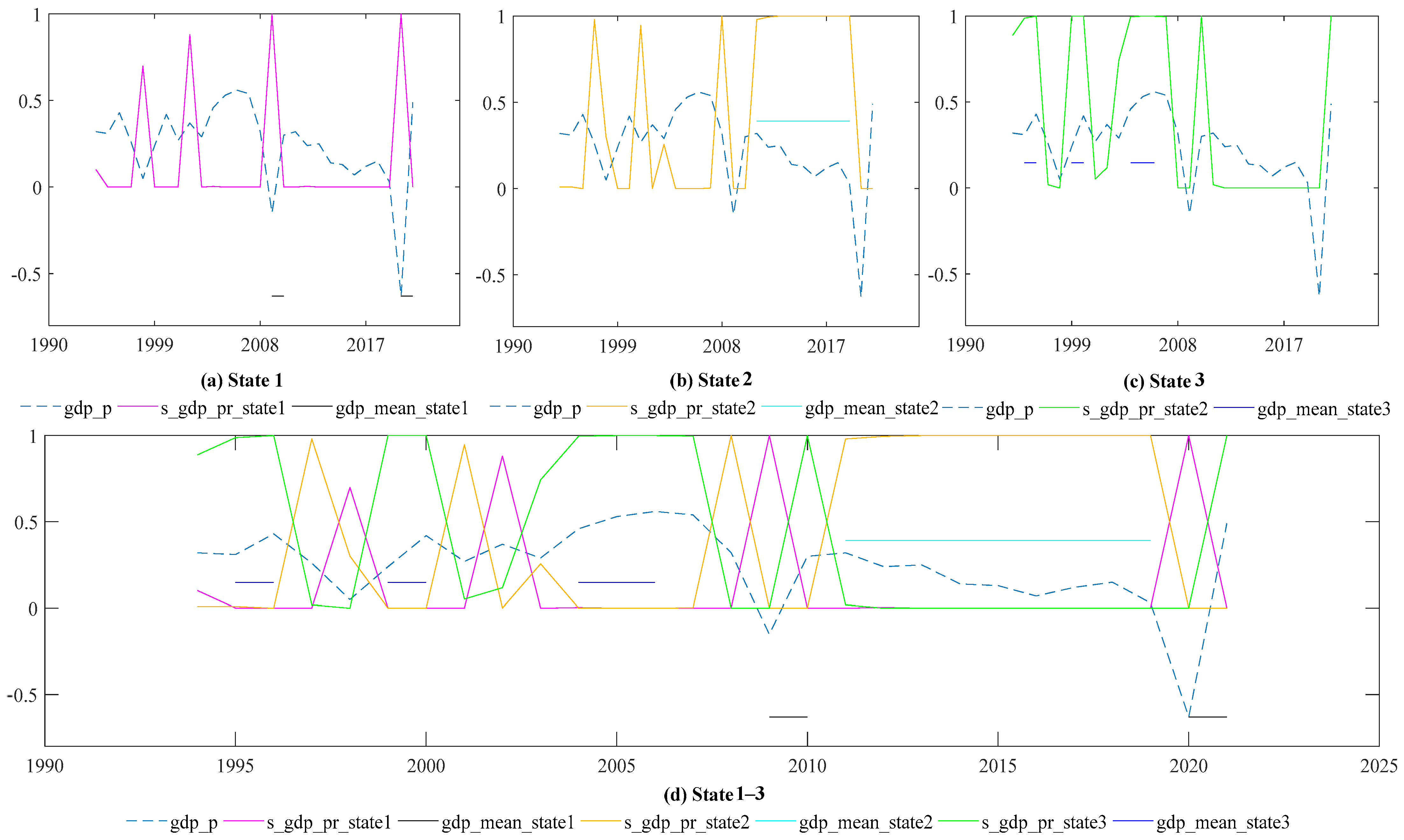
Figure 1 shows the filter transition probability from state 1 to state 3 as well as G D P . Figure 1, graph a, shows the state 1 filter transition probability for G D P . There is a weak transition probability for moving to state 2 in 1998 and 2002. The G D P moved to state 1 briefly in 2009 and 2021. Figure 1, graph b, shows the state 2 filter transition probability for G D P . The economy moved to state 2 four times, and the one possible fifth transition to the state was not successful. The times that the economy operated in state 2 were in 1997, 2001, and 2008, and from 2011 to 2019. The one time that the economy failed to be in state 2 was in 2003. Graph c in Figure 1 shows the state 3 filter transition probability for G D P . The economy moved to state 3 five times in 1995 to 1996, 1999 to 2000, 2004 to 2006, 2010, and 2021. Figure 1, graph d, shows all the different regimes combined with the repetitive mean for the GDP.
Table 7 shows the expected duration of each state. When the economy is in state 1, it is found to run for 1 year. State 2 is found to run for 2 years, and state 3 is found to run for 3 years.
Table 8 reflects the matrix of transition probabilities for economic growth in different states. The first state is characterized by a negative mean of 2.349%. In this state, the economy is found to have a transition probability of 0.2946238. This reflects that there is a 29.46% chance that the economy will move from state 1 and return to state 1. On the other hand, the second state is characterized by a mean of 1.129%. In this state, the economy is found to have a transition probability of 0.3407753. This reflects that there is a 34.07% chance that the economy will move from state 2 and return to state 2. The third state has a mean of 3.679%. In this state, the economy is found to have a transition probability of 0.5802805. This reflects that there is a 58.02% chance that the economy will move from state 3 and return to state 3. The highest rate is a 58.02% chance of staying in a state that has a positive economic growth rate of 3.67%. However, this rate is still not sufficient to solve the South African macroeconomic challenges. Therefore, even if the economy is operating in this state, fiscal authorities need to find ways to stimulate economic growth.
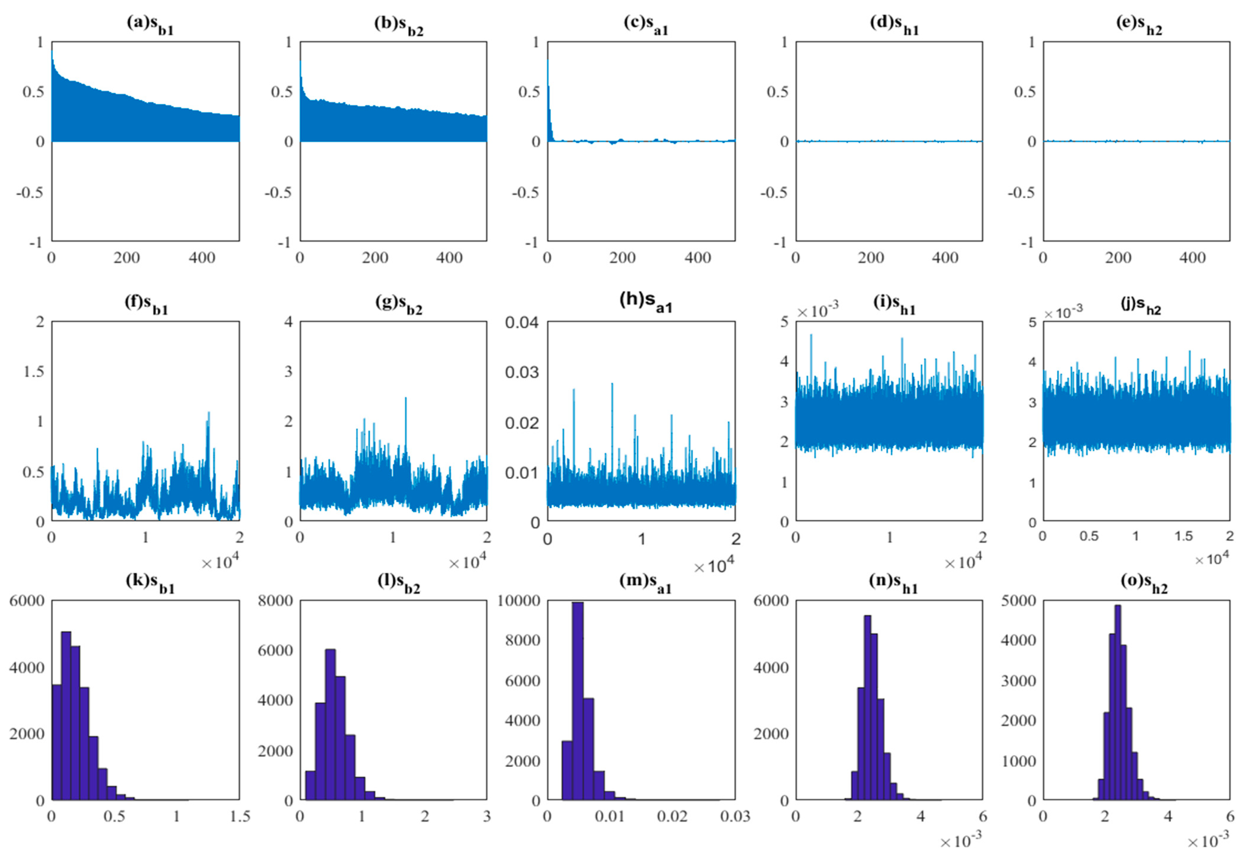
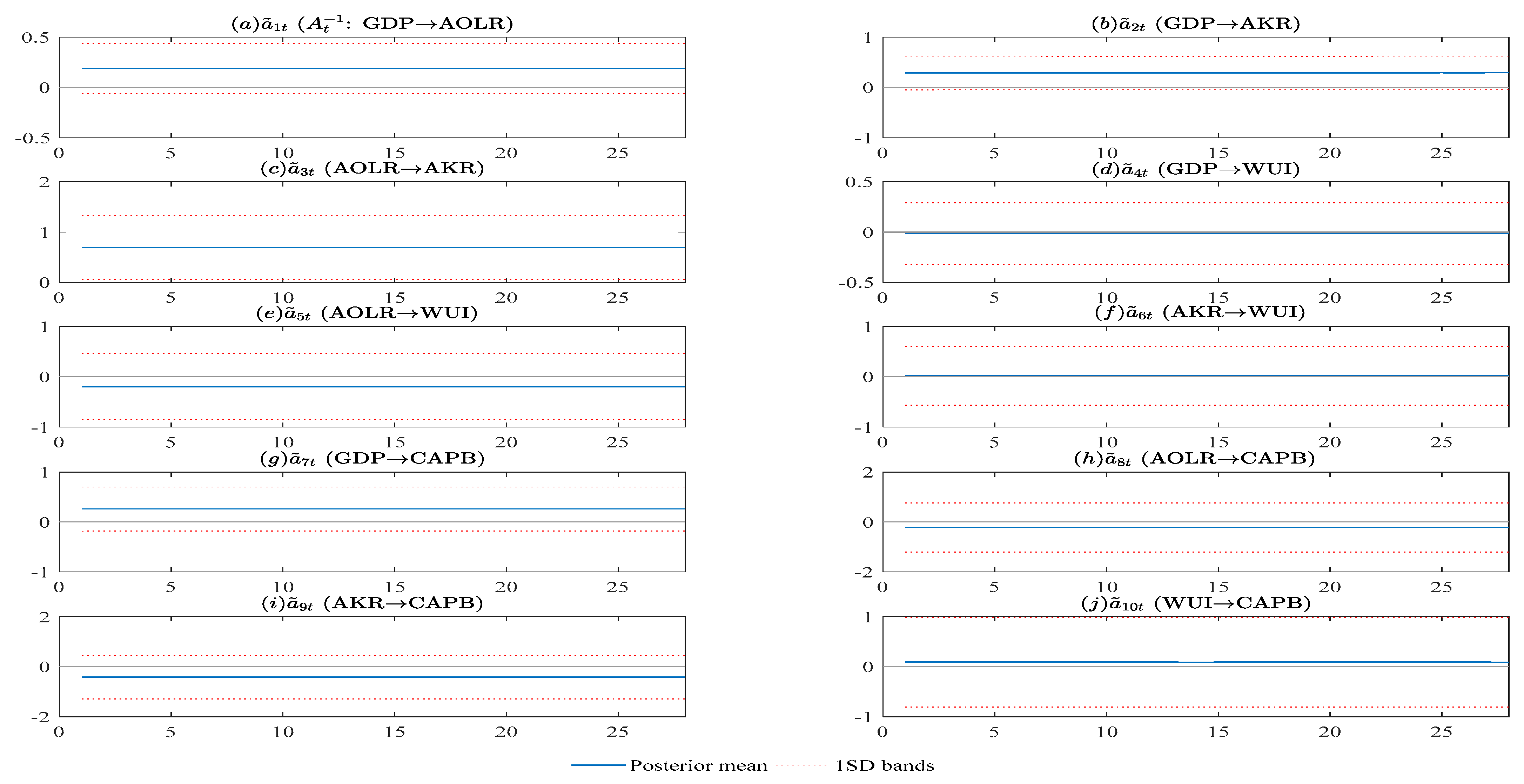
The TVP-VAR results are shown in Table 9, which shows the parameters, 95% confidence intervals, convergence diagnostics (CD) of Geweke (1992), and inefficiency factors computed using the MCMC sample. In the estimated result, the null hypothesis of convergence to the posterior distribution is not rejected for the parameters at the 5% significance level based on the CD statistics, and the inefficiency factors are quite low, except for sh2, which indicates efficient sampling for the parameters and the state variables. In the simulation in this paper, the priors are summed to follow the TVP regression model with stochastic volatility discussed above in Equation (21). 
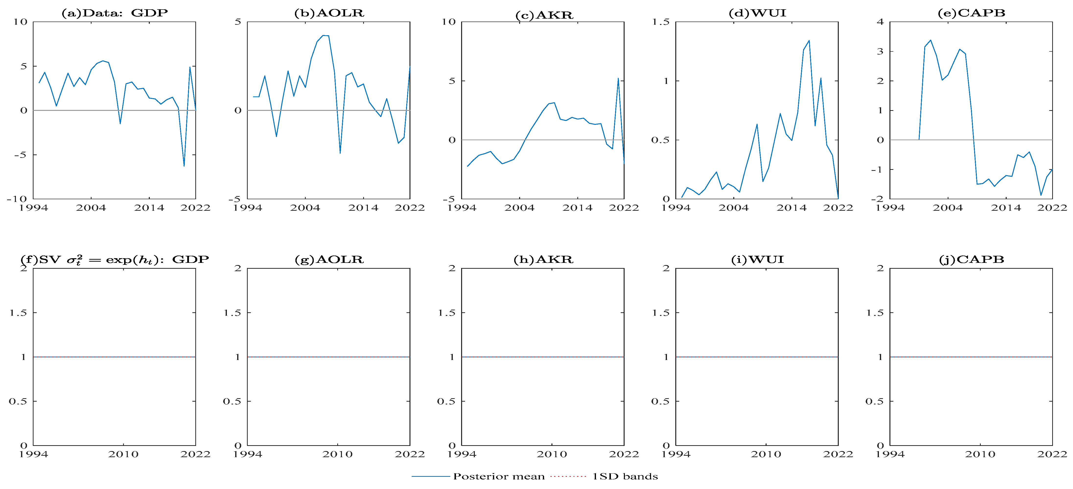
Table 9 reports the estimation results for the TVP regression model. The standard deviation is wider than the stochastic volatility model, and the posterior means are slightly apart from the true value.
Figure A2 reflect that the posterior means trace the movement of the true values, and the 95% credible intervals tend to be narrower overall than the constant volatility model, and almost include the true values. Figure 2 shows the sample autocorrelation function, the sample paths, and the posterior densities for the selected parameters. After discarding the initial 5000 samples in the burn-in period, the sample paths look stable, and the sample autocorrelations drop smoothly.
The properties of the state space model are reflected by the time-varying intercept in Figure A3. The lag-order selection criteria of (LR, FPE, AIC, HQIC, and SBIC) are presented in Table A1. The criteria LR, AIC, HQIC, and SBIC recommend the use of the optimal 4 lag. The paper concludes with an optimal 4. The results of the Johansen cointegration tests, in Table A2, show that the null hypothesis for the zero cointegrating equation is rejected at a 0.05 significance level. All of the trace statistics are greater than the critical value, therefore there is no long-run relationship. Therefore, the VAR in the TAP-VAR is valid to be used.
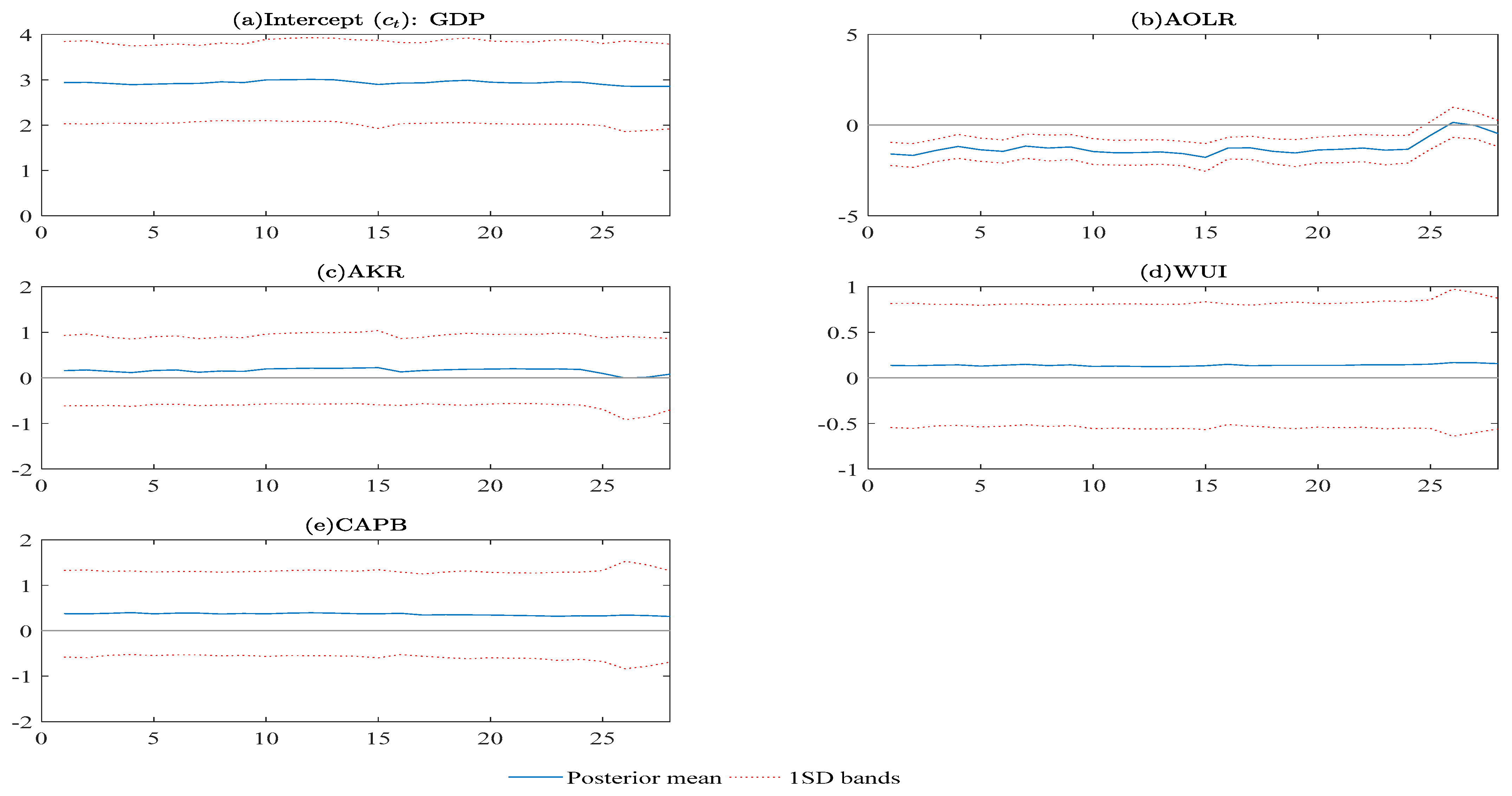
Figure 3 reflects the time-varying coefficient from 1994 to 2022. In graph p, there is a reflection of world uncertainty for South Africa. It is noted that, if uncertainty is expected in the next one- and three-year periods, it results in the economic growth operating below equilibrium. However, when uncertainty is expected in 6 years, the economic growth performs better. This may be because fiscal consolidation provides an accommodative policy and because there is an opportunity to implement better planning to account for the uncertainty when it is expected to occur far in the future. On the other hand, graph u reflects the impact of fiscal consolidation on economic growth. It is noted that, in the presence of fiscal consolidation, the economic growth operates above equilibrium. However, in the 1990 and 2000s, there is a reflection of volatility in economic growth. On the other hand, in recent times, economic growth is above the equilibrium in the presence of fiscal consolidation.
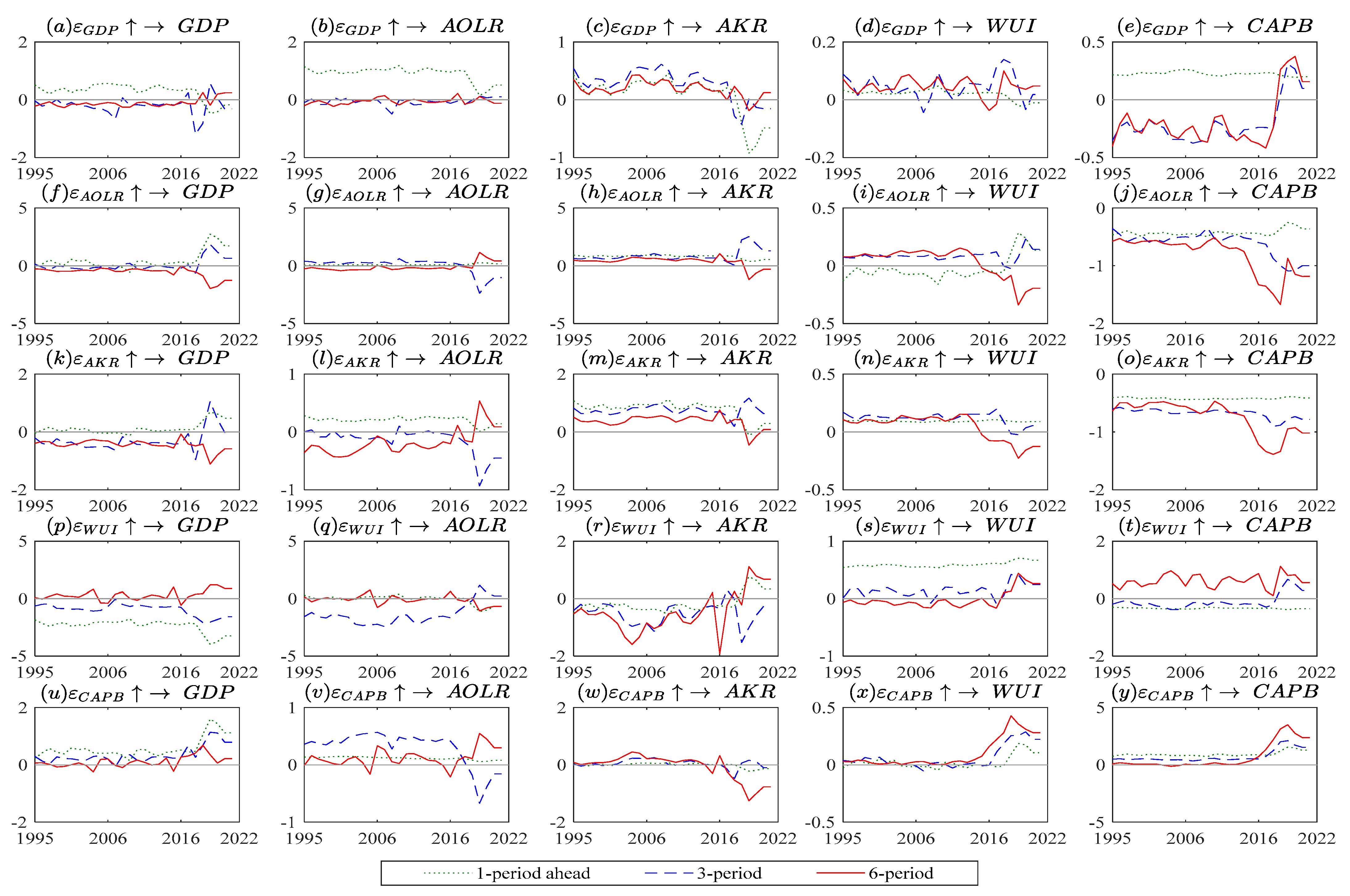
Figure 4 shows the time-varying impulse response functions. Figure 4, graph p provides evidence that the shock of macroeconomic uncertainty harms G D P . There is evidence that W U I results in a negative impact of 1.5% to 2.5% on G D P in years 1 and 2, respectively. This result is similar to those of Redl (2018), Bournakis and Ramirez-Rondan (2022), and Tunc et al. (2022), who found a negative impact for macroeconomic uncertainty on economic growth. The G D P is in the negative values until year 5, when G D P records a 1% increase; thereafter, G D P normalizes around the equilibrium. The time reach equilibrium is better by year 4, which is similar to the result obtained by Binge and Boshoff (2020). Figure 3, graph u provides evidence that the shock of fiscal consolidation, C A P B has a positive effect on G D P from year 1 to year 2 as G D P increases by 0.3 to 0.5%. However, after year 2, there is a drastic decrease in G D P to 0%, and then a further decrease of 0.2%. This are similar to the findings of Bardaka et al. (2021) and Caselli and Reynaud (2020), who note that fiscal consolidation has a negative impact on the gross domestic product. This may have critical implications and put the economy in recession. There is a possibility of a further negative effect on the economy if the recession occurred as a result of the adoption of fiscal consolidation. Nevertheless, G D P shows resilience, as it rebounds in year 5 with a positive rate of 0.1%. After that, G D P falls and does not return to equilibrium; it operates below the equilibrium level. This result suggests that fiscal consolidation cannot be used in the effort to stimulate economic growth.

5. Conclusions

There has been growing interest in the effort to investigate the impact of macroeconomic uncertainty on economic growth. However, there is no agreement in the findings of scholars as to what the impact of macroeconomic uncertainty on economic growth is. South Africa has been lagging in its efforts to achieve an economic growth rate of 5%, which is stipulated in the National Development Plan of 2013. On the other hand, fiscal authorities have been showing commitment to adopting fiscal consolidation. The issues with South Africa’s economy cannot be isolated to macroeconomic uncertainty. However, less attention has been given to the investigation of macroeconomic uncertainty in different regimes of economic growth in South Africa. The key contribution of this paper is to fill this gap in the effort to understand the impact of macroeconomic uncertainty in the presence of fiscal consolidation.
In this regard, it is important to investigate the impact of macroeconomic uncertainty on different regimes of economic growth in the presence of fiscal consolidation in South Africa. Markov-switching dynamic regression and time-varying vector autoregression (TA-VAR) were performed using time series data from 1994 to 2022. Three states are found for economic growth, with mean rates of negative 6.72%, 4.38% and 3.08% in the respective states. It is recommended that fiscal authorities revise the policy of the NDP with the key tangible target. The formulation of policy is critical in accounting for the state of the economy, as outlined above.
Macroeconomic uncertainty was found to have negative impacts of 6.729%, 4.385% and 3.080% in states 1 to 3, respectively. Fiscal consolidation provided an accommodative policy, as it reduced the negative impact of macroeconomic uncertainty by 3.57%, 1.996% and 0.92% in states 1 to 3, respectively. Investment and consumer expenditure may decline as a result of policy uncertainty, which might have a detrimental effect on economic growth. In the meantime, fiscal consolidation, which is the process of cutting government expenditure while raising income, can hinder economic development in the near term, since it decreases demand. On the other hand, fiscal consolidation has the potential to lower government debt over the long run, boost economic confidence, and produce a more stable political climate. These factors can drive spending and investment, which will ultimately result in better rates of economic growth. It is in this context that South African fiscal authorities and policymakers may face tradeoffs when trying to counter macroeconomic uncertainty. Therefore, further studies may be needed to ascertain the magnitude of the tradeoffs in order to make informed decisions.
Nevertheless, in this paper, it was found that fiscal consolidation does not completely reduce the negative impact of macroeconomic uncertainty. The transition probabilities of economic growth moving and returning to the same states are 29.46%, 34.07%, and 58.02% in each state, respectively. The time-varying impulse response functions showed that the shock of macroeconomic uncertainty harms economic growth. Nevertheless, the multiplier effect is not large; however, the economy operates below equilibrium and does not return to equilibrium after the effects of macroeconomic uncertainty. This reflects that it takes time for macroeconomic uncertainty to filter out of the South African economy. It is recommended that fiscal consolidation be considered as an accommodative fiscal policy to reduce macroeconomic uncertainty but not as a main policy for economic growth. The dummy variable C A P B _ S T B _ D U M M Y , reflecting the structural break of the fiscal consolidation, is found to have a positive impact on economic growth. This reflects that, in the case of a quick change or adoption of fiscal consolidation, there is a 1.962% chance that there will be an increase in economic growth. On the other hand, the W U I _ S T B _ D U M M Y structural break for macroeconomic uncertainty is found to result in a 3.765% chance of a fall in the gross domestic product. This reflects that unexpected change over time on macroeconomic uncertainty harms economic growth. South Africa fiscal author need to put in place economic model that can forecast unexpected change that can affect economic growth.

Funding

This research received no external funding.

Data Availability Statement

Not applicable.

Acknowledgments

I would like to acknowledge the Department of Economics at the University of Free State.

Conflicts of Interest

The authors declare no conflict of interest.

Appendix A

Table A1. Lag-order selection criteria.
LagLLLRDfpFPEAICHQICSBIC
0−137.746 5.3219215.860615.894716.108
1−62.5429150.41250.0000.0229510.2825 10.487211.7665
2−14.189596.707250.0000.0040637.687728.0628510.4083
31003.542035.5250.0003.7 × 10−49 *−102.616−102.07−98.6584
42686.423365.8 *250.0000.00000−288.491 *−287.878 *−284.04 *
* optimal lag.
Table A2. Johansen tests for cointegration.
Maximum RankParamsLLEigenvalueTrace StatisticCritical Value 5%
030−84.6960850.00000115.796968.52
139−62.1953710.8946170.795547.21
246−43.9378080.8389034.280329.68
351−35.086160.5873516.577015.41
454−29.1100180.449884.62483.76
555−26.7976390.20645
Figure A1. Posterior mean estimates for stochastic volatility. Actual data (top panels), posterior mean estimates for stochastic volatility of the structural shock for CPI (bottom panels). Note economic variables of G D P is gross domestic product, A O L R is average output labour ratio, A K R is average output capital ratio, W U I is world uncertainty for South Africa index, C A P B is cyclical adjusted primary balance (proxy fiscal consolidation).
Economies 11 00119 g0a1
Figure A2. Posterior and bands for volatility. Note economic variables of G D P is gross domestic product, A O L R is average output labour ratio, A K R is average output capital ratio, W U I is world uncertainty for South Africa index, C A P B is cyclical adjusted primary balance (proxy fiscal consolidation).
Economies 11 00119 g0a2
Figure A3. Posterior mean of time-varying intercept and bands for volatility. Note economic variables of G D P is gross domestic product, A O L R is average output labour ratio, A K R is average output capital ratio, W U I is world uncertainty for South Africa index, C A P B is cyclical adjusted primary balance (proxy fiscal consolidation).
Economies 11 00119 g0a3

References

  1. Ahiadorme, Johnson Worlanyo. 2022. On the aggregate effects of global uncertainty: Evidence from an emerging economy. South African Journal of Economics 90: 390–407. [Google Scholar] [CrossRef]
  2. Ahir, Hites, Nicholas Bloom, and Davide Furceri. 2022. The World Uncertainty Index. Working Paper 29763. Cambridge: National Bureau of Economic Research. [Google Scholar]
  3. Alesina, Alberto, and Silvia Ardagna. 2010. Large changes in fiscal policy: Taxes versus spending. Tax Policy and the Economy 24: 35–68. [Google Scholar] [CrossRef]
  4. Alesina, Alberto, Carlo Favero, and Francesco Giavazzi. 2019. Effects of austerity: Expenditure-and tax-based approaches. Journal of Economic Perspectives 33: 141–62. [Google Scholar] [CrossRef] [Green Version]
  5. Ardanaz, Martín, Eduardo Cavallo, Alejandro Izquierdo, and Jorge Puig. 2021. Growth-friendly fiscal rules? Safeguarding public investment from budget cuts through fiscal rule design. Journal of International Money and Finance 111: 102319. [Google Scholar] [CrossRef]
  6. Auerbach, Alan J., and Yuriy Gorodnichenko. 2017. Fiscal Stimulus and Fiscal Sustainability. No. w23789. Cambridge: National Bureau of Economic Research. [Google Scholar]
  7. Baker, Scott R., and Nicholas Bloom. 2013. Does Uncertainty Reduce Growth? Using Disasters as Natural Experiments. No. w19475. Cambridge: National Bureau of Economic Research. [Google Scholar]
  8. Baker, Scott R., Nicholas Bloom, and Steven J. Davis. 2016. Measuring economic policy uncertainty. The Quarterly Journal of Economics 131: 1593–636. [Google Scholar] [CrossRef]
  9. Baker, Scott R., Nicholas Bloom, Steven J. Davis, and Kyle J. Kost. 2019. Policy News and Stock Market Volatility. No. w25720. Cambridge: National Bureau of Economic Research. [Google Scholar]
  10. Balcilar, Mehmet, George Ike, and Rangan Gupta. 2022. The role of economic policy uncertainty in predicting output growth in emerging markets: A mixed-frequency granger causality approach. Emerging Markets Finance and Trade 58: 1008–26. [Google Scholar] [CrossRef]
  11. Balcilar, Mehmet, Rangan Gupta, and Theshne Kisten. 2021. The impact of uncertainty shocks in South Africa: The role of financial regimes. Review of Financial Economics 39: 442–54. [Google Scholar] [CrossRef]
  12. Ball, Laurence. 2014. Long-term damage from the Great Recession in OECD countries. European Journal of Economics and Economic Policies: Intervention 11: 149–60. [Google Scholar]
  13. Bardaka, Ioanna, Ioannis Bournakis, and Georgia Kaplanoglou. 2021. Total factor productivity (TFP) and fiscal consolidation: How harmful is austerity? Economic Modelling 94: 908–22. [Google Scholar] [CrossRef] [Green Version]
  14. Berger, Tino, Sibylle Grabert, and Bernd Kempa. 2017. Global macroeconomic uncertainty. Journal of Macroeconomics 53: 42–56. [Google Scholar] [CrossRef]
  15. Bhagat, Sanjai, Pulak Ghosh, and Srinivasan Rangan. 2016. Economic policy uncertainty and growth in India. Economic and Political Weekly 51: 72–81. [Google Scholar] [CrossRef] [Green Version]
  16. Bi, Huixin, Eric M. Leeper, and Campbell Leith. 2013. Uncertain fiscal consolidations. The Economic Journal 123: F31–F63. [Google Scholar] [CrossRef] [Green Version]
  17. Binge, Laurie H., and Willem H. Boshoff. 2020. Economic uncertainty in South Africa. Economic Modelling 88: 113–31. [Google Scholar] [CrossRef]
  18. Bloom, Nicholas. 2009. The impact of uncertainty shocks. Econometrica 77: 623–85. [Google Scholar]
  19. Bloom, Nicholas. 2014. Fluctuations in uncertainty. Journal of economic Perspectives 28: 153–76. [Google Scholar] [CrossRef] [Green Version]
  20. Bournakis, Ioannis, and Nelson R. Ramirez-Rondan. 2022. Does Uncertainty Matter for the Fiscal Consolidation and Capital Intensity Nexus? No. 111592. Munich: University Library of Munich. [Google Scholar]
  21. BR. 2014. Budget Review 2014. Pretoria: Communications Directorate, National Treasury. [Google Scholar]
  22. Brady, Gordon L., and Cosimo Magazzino. 2018. Government debt in EMU countries. The Journal of Economic Asymmetries 18: e00096. [Google Scholar] [CrossRef]
  23. Bredin, Don, and Stilianos Fountas. 2009. Macroeconomic uncertainty and performance in the European Union. Journal of International Money and Finance 28: 972–86. [Google Scholar] [CrossRef]
  24. Bredin, Don, John Elder, and Stilianos Fountas. 2009. Macroeconomic uncertainty and performance in Asian countries. Review of Development Economics 13: 215–29. [Google Scholar] [CrossRef]
  25. Burger, Philippe, and Chandapiwa Jimmy. 2006. Should South Africa have a fiscal rule? South African Journal of Economics 74: 642–69. [Google Scholar] [CrossRef]
  26. Caselli, Francesca, and Julien Reynaud. 2020. Do fiscal rules cause better fiscal balances? A new instrumental variable strategy. European Journal of Political Economy 63: 101873. [Google Scholar] [CrossRef] [Green Version]
  27. Chen, Lingtao, Yongna Yuan, and Na Zhao. 2022. The effect of oil price uncertainty on corporate investment in the presence of growth options: Evidence from listed companies in China (1998–2019). The North American Journal of Economics and Finance 62: 101779. [Google Scholar] [CrossRef]
  28. Cogan, John F., Daniel L. Heil, and John B. Taylor. 2020. A Pro-Growth Fiscal Consolidation Plan for the United States. Economics Working Paper 20114. Stanford: Hoover Institution. [Google Scholar]
  29. Fatima, Amber, and Abdul Waheed. 2011. Effects of Macroeconomic Uncertainty on Investment and Economic Growth: Evidence from Pakistan. Transition Studies Review 18: 112–23. [Google Scholar] [CrossRef]
  30. Fed USA. 2022. Economic Policy Uncertainty. Available online: https://fred.stlouisfed.org/series/WUIZAF (accessed on 12 November 2022).
  31. Fountas, Stilianos, and Menelaos Karanasos. 2006. The relationship between economic growth and real uncertainty in the G3. Economic Modelling 23: 638–47. [Google Scholar] [CrossRef]
  32. FRB. 2018. Fiscal Responsibility Bill. Pretoria: Communications Directorate, National Treasury. [Google Scholar]
  33. Gechert, Sebastian, Gustav Horn, and Christoph Paetz. 2019. Long-term effects of fiscal stimulus and austerity in Europe. Oxford Bulletin of Economics and Statistics 81: 647–66. [Google Scholar] [CrossRef]
  34. Geweke, John. 1992. Evaluating the accuracy of sampling-based approaches to the calculations of posterior moments. Bayesian Statistics 4: 641–49. [Google Scholar]
  35. Ghosh, Atish R., Jun I. Kim, Enrique G. Mendoza, Jonathan D. Ostry, and Mahvash S. Qureshi. 2013. Fiscal fatigue, fiscal space and debt sustainability in advanced economies. The Economic Journal 123: F4–F30. [Google Scholar] [CrossRef]
  36. Giavazzi, Francesco, and Marco Pagano. 1995. Non-Keynesian Effects of Fiscal Policy Changes: International Evidence and the Swedish Experience. Cambridge: National Bureau of Economic Research. [Google Scholar]
  37. Gründler, Klaus, and Niklas Potrafke. 2020. Fiscal Rules: Historical, Modern, and Sub-National Growth Effects. CESifo Working Paper No. 8305. Munich: CESifo GmbH. [Google Scholar]
  38. Gupta, Rangan, and Charl Jooste. 2018. Unconventional monetary policy shocks in OECD countries: How important is the extent of policy uncertainty? International Economics and Economic Policy 15: 683–703. [Google Scholar] [CrossRef]
  39. Hamilton, James D. 1989. A new approach to the economic analysis of nonstationary time series and the business cycle. Econometrica: Journal of the Econometric Society 40: 357–84. [Google Scholar] [CrossRef]
  40. Hamilton, James D. 1990. Analysis of time series subject to changes in regime. Journal of Econometrics 45: 39–70. [Google Scholar] [CrossRef]
  41. Hansen, Bruce E. 1996. Inference when a nuisance parameter is not identified under the null hypothesis. Econometrica: Journal of The Econometric Society 64: 413–30. [Google Scholar] [CrossRef] [Green Version]
  42. Hansen, Bruce E. 2000. Sample splitting and threshold estimation. Econometrica 68: 575–603. [Google Scholar] [CrossRef] [Green Version]
  43. Heimberger, Philipp. 2017. Did fiscal consolidation cause the double-dip recession in the euro area? Review of Keynesian Economics 5: 439–58. [Google Scholar] [CrossRef] [Green Version]
  44. Herwartz, Helmut, and Bernd Theilen. 2022. Effectiveness and counter-cyclicality of fiscal consolidation under compliance regulation: The case of the Stability and Growth Pact. Economics & Politics, 1–25. [Google Scholar] [CrossRef]
  45. IMF. 2010. Will It Hurt? Macroeconomic Effects of Fiscal Consolidation. IMF World Economic Outlook 93: 124. [Google Scholar]
  46. IMF. 2020. Cyclically Adjusted Balance. Available online: https://www.imf.org/external/datamapper/GGCB_G01_PGDP_PT@FM/ADVEC/FM_EMG/ (accessed on 11 August 2022).
  47. Johannsen, Benjamin K. 2014. When Are the Effects of Fiscal Policy Uncertainty Large? (No. 2014-40). Washington, DC: Board of Governors of the Federal Reserve System. [Google Scholar]
  48. Jordà, Òscar, and Alan M. Taylor. 2016. The time for austerity: Estimating the average treatment effect of fiscal policy. The Economic Journal 126: 219–55. [Google Scholar] [CrossRef] [Green Version]
  49. Kisten, Theshne. 2020. Macroeconomic implications of uncertainty in South Africa. South African Journal of Economic and Management Sciences 23: 1–15. [Google Scholar] [CrossRef]
  50. Koop, Gary, and Dimitris Korobilis. 2018. Variational Bayes Inference in High-Dimensional Time-Varying Parameter Models. No. 87972. Munich: University Library of Munich. [Google Scholar]
  51. Kotze, Kevin. 2017. Fiscal Policy Uncertainty and Economic Activity in South Africa. School of Economics Macroeconomic Discussion Paper Series 2; Rondebosch: University of Cape Town. [Google Scholar]
  52. Kumo, Wolassa L. 2006. Macroeconomic uncertainty and aggregate private investment in South Africa. South African Journal of Economics 74: 190–204. [Google Scholar] [CrossRef]
  53. Long, Shaobo, and Rui Zhang. 2022. The asymmetric effects of international oil prices, oil price uncertainty and income on urban residents’ consumption in China. Economic Analysis and Policy 74: 789–805. [Google Scholar] [CrossRef]
  54. Madanizadeh, Seyed Ali, and Abolfazl Setayesh. 2020. Macroeconomic Uncertainty and Economic Development. Tehran: Sharif University of Technology. [Google Scholar]
  55. Mandeya, Shelton Masimba Tafadzwa, and Sin-Yu Ho. 2021. Inflation, inflation uncertainty and the economic growth nexus: An impact study of South Africa. MethodsX 8: 101501. [Google Scholar] [CrossRef]
  56. Mankiw, N. Gregory. 2019. Brief Principles of Macroeconomics. Boston: Cengage Learning. [Google Scholar]
  57. MTBPS. 2014. Medium Term Budget Policy Statement 2014. Pretoria: Communications Directorate, National Treasury. [Google Scholar]
  58. Mtibaa, Ameni, Amine Lahiani, and Foued Badr Gabsi. 2022. Impact of fiscal consolidation on economic growth: The Tunisian case. The Journal of Risk Finance 23: 558–82. [Google Scholar] [CrossRef]
  59. Mumtaz, Haroon, and Konstantinos Theodoridis. 2017. Common and country specific economic uncertainty. Journal of International Economics 105: 205–16. [Google Scholar] [CrossRef]
  60. Mumtaz, Haroon, and Konstantinos Theodoridis. 2018. The changing transmission of uncertainty shocks in the US. Journal of Business & Economic Statistics 36: 239–52. [Google Scholar]
  61. Mumtaz, Haroon. 2016. The evolving transmission of uncertainty shocks in the United Kingdom. Econometrics 4: 16. [Google Scholar] [CrossRef] [Green Version]
  62. Nakajima, Jouchi. 2011. Time-varying parameter VAR model with stochastic volatility: An overview of methodology and empirical applications. Monetary and Economic Studies 29: 107–42. [Google Scholar]
  63. National Planning Commission. 2013. National Development Plan Vision 2030. Pretoria: Communications Directorate, National Treasury. [Google Scholar]
  64. Olanipekun, Ifedolapo Olabisi, Hasan Güngör, and Godwin Olasehinde-Williams. 2019. Unraveling the causal relationship between economic policy uncertainty and exchange market pressure in BRIC countries: Evidence from bootstrap panel granger causality. Sage Open 9: 2158244019853903. [Google Scholar] [CrossRef] [Green Version]
  65. Olaoye, Olumide Olusegun, and Philip A. Olomola. 2022. Empirical analysis of asymmetry phenomenon in the public debt structure of Sub-Saharan Africa’s five biggest economies: A Markov-Switching model. The Journal of Economic Asymmetries 25: e00242. [Google Scholar] [CrossRef]
  66. Primiceri, Giorgio E. 2005. Time varying structural vector autoregressions and monetary policy. The Review of Economic Studies 72: 821–52. [Google Scholar] [CrossRef]
  67. Rasmidatta, Pinchawee. 2011. The Relationship between Domestic Saving and Economic Growth and Convergence Hypothesis: Case Study of Thailand. Huddinge: Department of Economics, Sodertorns University. [Google Scholar]
  68. Redl, Chris. 2018. Macroeconomic uncertainty in South Africa. South African Journal of Economics 86: 361–80. [Google Scholar] [CrossRef]
  69. SARB. 2022. Online Statistical Query (Historical Macroeconomic Timeseries Information). Available online: https://www.resbank.co.za/Research/Statistics/Pages/OnlineDownloadFacility.aspx (accessed on 11 November 2022).
  70. Sims, Christopher A. 1980. Martingale-Like Behavior of Prices. NBER Working Paper (w0489). Cambridge: National Bureau of Economic Research Cambridge. [Google Scholar]
  71. Swanepoel, Jan, and Nicolaas Johannes Schoeman. 2003. Countercyclical fiscal policy in South Africa: Role and impact of automatic fiscal stabilisers. South African Journal of Economic and Management Sciences 6: 802–22. [Google Scholar] [CrossRef]
  72. Tunc, Ahmet, Mustafa Kocoglu, and Alper Aslan. 2022. Time-varying characteristics of the simultaneous interactions between economic uncertainty, international oil prices and GDP: A novel approach for Germany. Resources Policy 77: 102658. [Google Scholar] [CrossRef]
  73. World Bank. 2022. Data Bank World Development Indicators. Available online: https://databank.worldbank.org/indicator/NY.GDP.MKTP.KD.ZG/1ff4a498/Popular-Indicators (accessed on 11 November 2022).
  74. Wu, Xi, and Yudong Wang. 2021. How does corporate investment react to oil prices changes? Evidence from China. Energy Economics 97: 105215. [Google Scholar] [CrossRef]
Figure 1. States 1 to 3: filter transition probabilities and GDP. Note: g d p _ p is the gross domestic product, s _ g d p _ p _ p r _ s t a t e 1 reflect state one filter transition probabilities, s _ g d p _ p _ p r _ s t a t e 2   s t a t e 1 reflect state two filter transition probabilities, s _ g d p _ p _ p r _ s t a t e 3   s t a t e 1 reflect state three filter transition probabilities, g d p _ m e a n _ s t a t e 1 is the mean of gross domestic product in state one, g d p _ m e a n _ s t a t e 2 is the mean of gross domestic product in state two, and g d p _ m e a n _ s t a t e 3 is the mean of gross domestic product in state three.
Economies 11 00119 g001
Figure 2. Estimates of the moments and posterior distributions of the model. Note: Sample autocorrelations (top), sample paths (middle), and posterior densities (bottom).
Economies 11 00119 g002
Figure 3. Time-varying coefficient. Note economic variables of G D P is gross domestic product, A O L R is average output labour ratio, A K R is average output capital ratio, W U I is world uncertainty for South Africa index, C A P B is cyclical adjusted primary balance (proxy fiscal consolidation).
Economies 11 00119 g003
Figure 4. Time-varying impulse response functions. Note economic variables of G D P is gross domestic product, A O L R is average output labour ratio, A K R average output capital ratio, W U I is world uncertainty for South Africa index, C A P B is cyclical adjusted primary balance (proxy fiscal consolidation).
Economies 11 00119 g004
Table 1. Economic variables.
Economic VariablesDescriptionSourced
G D P Gross domestic productSouth African Reserve Bank
A O L R Average output labour ratioSouth African Reserve Bank
A K R Average output capital ratioSouth African Reserve Bank
W U I World uncertainty for South Africa indexFed USA, Ahir et al. (2022)
C A P B Cyclical adjusted primary balance (proxy fiscal consolidation).International Monetary Fund IMF (2020)
V S P   The volatility of the stock price index for South AfricaFed USA, Baker et al. (2019)
E M V Equity market volatility tracker: Fiscal policy, indexFed USA
E P U Economic policy uncertainty index: Monetary policyFed USA
S W U I Smoothed world uncertainty index for South Africa Fed USA, Ahir et al. (2022)
G E P R Government Effectiveness: PercentileWB, Worldwide Governance Indicators
P S A V Political Stability and Absence of Violence/Terrorism: Standard ErrorWB, Worldwide Governance Indicators
C A P B _ S T B _ D U M M Y The dummy variable of a proxy structural break for Cyclical adjusted primary balance (which measures fiscal consolidation).Estimated
W U I _ S T B _ D U M M Y Dummy variable of a proxy structural break for World uncertainty for the South Africa indexEstimated
The data sourced: SARB (2022), World Bank (2022), IMF (2020), and Fed USA (2022).
Table 2. Descriptive statistics.
Economic VariableObsMeanStd. Dev.MinMax
G D P 282.4392862.408832−6.35.6
A O L R   291.0771031.699371−2.417514.22754
A K R 290.3060321.986146−2.242955.218176
W U I 290.395970.363260.0126461.34288
C A P B   290.3081441.946491−1.875113.379194
V S P 2418.848935.23990311.1566334.10648
E M V 297.2730131.8794574.260511.10813
E P U 2987.8254432.8784239.49183168.6201
S W U I 293.3072032.76922208.745708
G E P R 209.61.353358711
P S A V 2054.049356.61434533.4905767.14976
Economic VariablesSkewness/Kurtosis Tests for Normality
ObsPr(Skewness)Pr(Kurtosis)adj chi2(2)Prob > chi2
G D P 280.00050.001616.330.0003
A O L R   290.82110.97690.050.9744
A K R 290.27820.53791.680.4311
W U I 280.00840.20467.480.0238
C A P B   230.25480.00099.930.0070
V S P   240.02160.08727.220.0271
E M V 290.51240.37481.310.5204
E P U 290.07540.64683.690.1579
S W U I 290.11430.24314.070.1305
G E P R 200.14600.54112.810.2448
P S A V 200.02350.00699.980.0068
H0 there is a normal distribution. H1 there is no normal distribution.
Table 3. Correlation among economic variables.
Economic Variable G D P A O L R A K R W U I C A P B V S P E M V E P U S W U I G E P R P S A V
G D P 1
A O L R   0.601
A K R 0.02−0.101
W U I −0.30−0.300..251
C A P B   0.690.58−0.49−0.471
V S P   −0.31−0.050.19−0.36−0.071
E M V −0.30−0.14−0.12−0.05−0.280.221
E P U −0.26−0.12−0.40−0.220.060.450.651
S W U I −0.47−0.280.260.86−0.53−0.320.15−0.161
G E P R −0.22−0.170.730.66−0.62−0.26−0.24−0.610.641
P S A V 0.510.560.40−0.240.250.070.020.04−0.230.091
Number of obs = 28.
Table 4. Dickey-Fuller test for unit root and structural break.
Economic VariableDickey-Fuller Test for Unit RootEconomic VariableStructural Break
Test Statistics1% Critical Value5% Critical Value10% Critical ValueStatisticp-ValueEstimated Break Date
G D P Z(t)−3.96−3.736−2.994−2.628 G D P 46.38430.00002017
A O L R   Z(t)−3.09−3.73−2.992−2.626 A O L R   93.76300.00002010
D . A K R Z(t)−8.326−3.736−2.994−2.628 A K R 102.34390.00002012
D . W U I Z(t)−6.286−3.743−2.997−2.629 D . A K R 396.82260.00002017
D . C A P B   Z(t)−3.081−3.75−3−2.63 W U I 44.16410.00002009
D . V S P Z(t)−4.339−3.750−3.000−2.630 D . W U I 98.77110.00002017
E M V Z(t)−3.182−3.730−2.992−2.626 C A P B   171.09490.00002009
E P U Z(t)−3.182−3.730−2.992−2.626 D . C A P B 48.92180.00002012
D . S W U I Z(t)−6.481−3.736−2.994−2.628 V S P   20.58530.00092005
D . G E P R Z(t)−3.450−3.750−3.000−2.630 E M V 865.92790.00001999
P S A V Z(t)−3.410−3.750−3.000−2.630 E P U 219.31940.00001999
S W U I 81.08970.00002016
G E P R 9.48510.11622019
P S A V 5.51430.48002017
Number of obs = 21 and MacKinnon approximate p-value for Z(t) = 0.0280.
Table 5. Markov-switching dynamic regression for macroeconomic uncertainty.
Economic Variables12345
G D P G D P G D P G D P G D P
A O L R 0.171 **0.229 ***−0.128 *−0.228 *
(2.81)(7.08)(−2.25)(−2.53)
A K R 0.737 ***0.314 ***0.897 ***0.751 ***
(10.77)(10.34)(15.83)(5.61)
C A P B _ S T B _ D U M M Y 1.962 ***
(4.67)
W U I _ S T B _ D U M M Y −3.765 ***
(−7.73)
State1
C A P B 2.127 *** 4.406 ***2.880 **
(21.68) (14.18)(2.68)
W U I −6.729 ***−0.8992.220
(−16.65)(−1.86)(1.25)
_ c o n s −6.299 ***−1.243 ***1.271 ***2.798 ***−1.772
(−5.43)(−6.39)(4.53)(4.46)(−0.68)
State2
C A P B 0.930 *** 0.707 ***1.047 ***
(11.94) (4.01)(6.15)
W U I −4.385 ***−0.277−1.209 **
(−12.25)(−0.82)(−2.68)
_ c o n s 3.910 ***0.879 ***3.242 ***1.002 **2.200 ***
(9.14)(6.37)(22.51)(2.78)(5.82)
State3
C A P B 0.919 *** 0.563 ***0.845 ***
(9.86) (7.58)(7.90)
W U I −3.080 ***−3.524 ***−1.275 **
(−15.94)(−5.37)(4.62)
_ c o n s 1.476 **2.415 ***4.710 ***4.242 ***3.596 ***
(2.71)(16.49)(38.35)(14.65)(11.46)
N2822272222
t statistics in parentheses. * p < 0.05, ** p < 0.01, *** p < 0.001.
Table 6. Markov-switching dynamic regression with extended proxies of uncertainty.
Economic
Variables
1234Economic
Variables
56
G D P G D P G D P G D P G D P G D P
A O L R −0.130−0.0259−0.366 ***−0.0908 ** A O L R −0.392 ***−0.0441
(−0.81)(−0.28)(−7.42)(−1.63) (−4.89)(−0.38)
A K R 0.687 ***0.685 ***0.778 ***0.677 *** A K R 0.449 **0.708 ***
(4.70)(6.59)(14.47)(11.93) (2.76)(6.82)
State1 State1
C A P B 3.103 ***2.326 ***2.294 ***1.618 *** P S A V −0.630 ***
(3.81)(13.83)(36.25)(20.53) (−4.47)
V S P −0.211 *** C A P B 3.043 ***1.903 ***
(−4.24) (25.10)(12.64)
E M V −0.271 *** W U I 3.102 ***2.295 ***
(−8.34) (6.47)(5.51)
E P U −0.0344 *** G E P R 1.119 ***
(−14.62) (3.36)
S W U I −0.456 ***
(−4.49)
_ c o n s 4.8081.5063.017 ***−0.0495 _ c o n s −2.051 ***−2.211 ***
(5.6.)(7.4)(13.00)(−0.12) (−7.85)(−5.55)
State2 State2
C A P B 1.350 ***1.155 ***1.363 ***0.944 *** P S A V −0.0526 *
(3.41)(10.24)(17.45)(12.01) (−2.10)
V S P −0.150 *** C A P B 1.335 ***0.974 ***
(−4.52) (12.03)(6.68)
E M V 0.00775 W U I −1.832 **−0.380
(0.06) (−3.23)(−0.66)
E P U −0.00380 G E P R 0.291
(−0.94) (1.54)
S W U I −0.216 ***
(−7.45)
_ c o n s 3.812 ***1.0382.072 ***2.567 *** _ c o n s 3.346 ***1.503 **
(7.20)(1.08)(4.93)(15.06) (4.79)(2.73)
State3 State3
C A P B 0.858 ***1.228 ***2.5300.782 P S A V 0.133 ***
(5.36)(6.48)(1.83)(1.02) (3.54)
V S P −0.119 C A P B 0.901 ***1.199 ***
(−1.62) (4.10)(4.20)
E M V 0.295 * W U I 2.2981.925
(2.25) (1.35)(1.10)
E P U 0.0422 *** G E P R 0.114
(4.88) (0.51)
S W U I −0.188
(−0.30)
_ c o n s −0.924 ***−0.895 ***−1.408 ***−1.539 *** _ c o n s 2.512 ***1.998 ***
(−5.32)(−5.55)(−9.06)(−8.57) (3.84)(3.33)
29292929 2929
t statistics in parentheses. * p < 0.05, ** p < 0.01, *** p < 0.001.
Table 7. Expected duration.
StateEstimateStd. Err.[95% Conf. Interval]
State11
State22.8458031.091730.7060524.985555
State33.0259811.4072260.2678695.784094
Number of obs = 28.
Table 8. Matrix of transition probabilities.
State123
State10.29462380.70357880.0017974
State20.24466510.34077530.4145597
State30.0025440.41971950.5802805
Table 9. Estimated parameters in the TVP-VAR model.
ParameterMeanStdev95% U95% LGewekeInef.
sb10.19370.11750.02980.47280.409206.57
sb20.55930.21420.2021.03910.841148.62
sa10.00550.00170.00340.00960.1199.93
sh10.00240.00030.00190.00310.120.54
sh20.00240.00030.00190.00310.7621.11
TVP-VAR model (Lag = 1)Iteration: 20,000
Notes: Mean, Stdev, and Inef represent posterior means, standard deviations, and the inefficiency factors, respectively.
Disclaimer/Publisher’s Note: The statements, opinions and data contained in all publications are solely those of the individual author(s) and contributor(s) and not of MDPI and/or the editor(s). MDPI and/or the editor(s) disclaim responsibility for any injury to people or property resulting from any ideas, methods, instructions or products referred to in the content.

