Article

Testing the Validity of the Quantity Theory of Money on Sectoral Data: Non-Linear Evidence from South Africa

by
Siyabonga Mndebele
,
Devi Datt Tewari
and
Kehinde Damilola Ilesanmi
*
Department of Economics, Faculty of Commerce, Administration, and Law, University of Zululand, KwaDlangezwa 3886, South Africa
*
Author to whom correspondence should be addressed.
Economies 2023, 11(2), 71; https://doi.org/10.3390/economies11020071
Submission received: 28 November 2022 / Revised: 17 January 2023 / Accepted: 6 February 2023 / Published: 20 February 2023
(This article belongs to the Special Issue International Financial Markets and Monetary Policy 2.0)

Abstract

:
Purpose: The purpose of this study is to test the validity of the quantity theory of money (QTM) on South African sectoral data. The rationale of this study and its necessity for South Africa as the case study is that, although aggregate inflation may lie within the target range, inflation at a sectoral level, particularly in the food and transport sector, is still a matter of concern in South Africa. Methodology/approach: This study employed the Non-linear Autoregressive Distributed Lagged model (NARDL) to assess potential asymmetries in the effect of money supply to differentiate between the effects of contractional and expansional episodes on inflation at the sectoral level. Quarterly time series data spanning from 2002Q2 to 2021Q2 was utilised for the estimation. Ultimately, the causal effect amongst the variables is examined by employing the Pairwise Granger Causality test. Findings: The results suggest that in the short run, the effect of monetary policy shocks is very weak. On the other hand, in the long run, both negative and positive shocks in the money supply push inflation at the sectoral level in the opposite directions, and positive shocks (expansionary monetary policy) have a greater effect than negative shocks, which renders the QTM invalid in South Africa. The sectoral response was found to be heterogeneous in the long run, and this was also backed by the results of the Granger Causality test and the dynamic multipliers. Asymmetry in the effect of the money supply is assessed in some of the sectors only in the long run. Practical implications: Based on the results, this study confirms great discrepancies in sectoral responses. Therefore, aggregate inflation may not be a good indicator of the inflation path in South Africa, as it may underestimate sectoral variations. Originality/value: The originality of this study lies on testing the validity of the QTM on inflation at the sectoral level in the South African context using a non-linear approach to assess potential asymmetry between the effects of expansionary and contractionary episodes of monetary policy shocks.

1. Introduction

The existing literature ascertains that combating inflation has been a matter of concern in emerging economies, since inflation is undesirable from both a macroeconomic and microeconomic standpoint (Katria et al. 2011). High inflation is not conducive to economic development, it weakens the value of a currency in terms of savings and demand, and it prevents economic agents from meeting their needs with the available money (Mahyar 2017). Therefore, the monetary policy focus should be centred on the pursuit of low inflation. As a result, in the year 2000, the South African Reserve Bank (SARB) has embarked on a huge decision to change its monetary policy framework and adopted a new monetary policy structure named “Inflation Targeting”, which is centred on the pursuit of low inflation by assuring that it ranges between the targets of 3% to 6%. On the other hand, achieving low inflation is among the goals of the National Development Plan (NDP) to be achieved by the year 2030. This background attests that emerging economies such as South Africa have given paramount importance to inflation.
Before the adoption of inflation targeting in the year 2000, South Africa experienced a high amount of inflation. The 1980s marked the highest inflation in South Africa since 1960 up to date. During the periods of the cash reserve-based regime, inflation reached 18.65%, the highest in its history. This was due to the 1979 oil crisis, which triggered the 1980 global recession, which played a major role in influencing inflation during this period. However, after the year 2000, when inflation targeting was adopted, inflation has been stable in South Africa. According to the Business Tech first quarter report of 2022, South Africa holds the record of being amongst the few countries, including China, Vietnam, and Indonesia, that have managed to keep their inflation stable. Specifically, South Africa has been successful in maintaining the inflation target of 3 to 6 per cent, which is below those of advanced economies, such as Hungary, US, Poland, UK, and the Eurozone.
Besides the success of monetary authorities at keeping aggregate inflation stable since the year 2000, inflation at a sectoral level in South Africa has been characterised by great discrepancies, and this worsened even further after the outbreak of COVID-19. Table 1 depicts the percentage weights in a descending order that were contributed by each sector in the 2021 Consumer Price Index (CPI) basket.
The housing and energy sector, transport sector, food and non-alcoholic beverages sector, and health sector weigh 42.4%, 18.2%, 14.3%, and 8.5%, respectively. These sectors have been described as the most expensive sectors in South Africa by STATSA. Moreover, Imbs et al. (2011) documented that in most developing economies, including South Africa, price elasticity tends to vary amongst sectors of the economy, resulting from the kinds of shocks each sector is subjected to.
After the outbreak of COVID-19, the Monetary Policy Committee (MPC) announced that they would fix the repo rate to influence money in circulation (money supply) in order to control the inflation pressure and stimulate economic activities. However, inflation in some sectors, especially the food and transport sectors remains high even to date. Could this imply that money supply is no longer the source of inflation or could this mean that the response of different sectors varies from money supply? These two questions remain unanswered, and therefore, form important objectives of this study. On the other hand, the history of these two variables (money supply and inflation) is well articulated by QTM, which serves as the fundamental theory that proposes a directly proportionate relationship between the stock of money in circulation (money supply) and inflation. Therefore, according to this theory, money supply can be used to control inflation. Although this theory has accorded a great deal of acceptance in empirical literature; nonetheless, in the modern unconventional monetary policy, the theory has lost its credibility. The Taylor rule framework is predominantly preferred by most central banks, particularly those using inflation targeting as monetary policy, such as in South Africa. Moreover, Cooray and Khraief (2018) have postulated that the direct relationship proposed by QTM may not hold during recessions, as expansionary monetary policies may have little impact on price variation as compared to during an expansion (liquidity trap). Therefore, it becomes crucial to consider the passthrough effect of monetary policy when studying these variables. Ultimately, monetary authorities in South Africa ought to seek other tools to combat inflationary pressure during the periods of economic downturns (recession) rather than the repo rate.
In this regard, the hypothesis tested by this study is the validity of the QTM on South African sectoral data, employing the Nonlinear Autoregressive Distributed Lagged model (NARDL). This contrasts previous studies (Perevalov and Maier 2010; Ofori et al. 2017; Adusei 2013; Alemu et al. 2016 among others) that employed aggregate inflation to study this relationship, which underestimate sectoral variations and might have confounded the results of previous studies on this relationship, which lead to the inflation paradox. This model will play a role to distinguish the effect of both contractional and expansional episodes of monetary policy employed by SARB during the period under investigation, in order to assess potential asymmetry. The rationale and necessity of this study emanates from the fact that sectoral inflation is inconsistent with aggregate inflation in South Africa, and there are discrepancies in the sectoral response, signalling the possibility of asymmetry in the effect money supply. The empirical literature provides limited evidence of the effect of money supply on sectoral inflation, and this proves to be a gap in the literature, because the success of monetary policy may be traced through stability in sectoral inflation (which lies between 3 and 6%) and fewer discrepancies. Distinct from previous studies, this study contributes to existing knowledge by evaluating the influence of money supply on inflation at the sectoral level rather than aggregate inflation. Disaggregate data provide more variations through which reliable inferences will be estimated. Furthermore, this study contributes by distinguishing the effect of monetary policy on inflation by the episodes of expansionary and contractionary monetary policies by the SARB. The remainder of this paper proceeds as follows: Section 2 covers the literature review, the methodology is highlighted in Section 3, Section 4 provides empirical results, and Section 5 outlines the summary and policy implications.

2. Literature Review

Serving as the foundation theory instigating the correlation between money supply and inflation, the QTM is carefully chosen as the theory that will underpin this study as the widely accepted schools of thought in the money supply and inflation relationship in the field of monetary policy (Wang 2017). The QTM provided the main conceptual framework for the interpretation of modern financial events. It then formed the principal core of the classical monetary evaluation of the 19th century and shaped the coherent prescription underpinning the conventional monetary policy. David Hume established the first dynamic process by breaking down how the effect of a change in monetary policy is transmitted from one sector to another in the economy, changing the relative price and quantity in the process (Atkin and La Cava 2017). He provided significant refinement and explanation and made a tremendous contribution to the quantity theory of money.
According to the QTM through the work of Friedman (1989), “inflation is everywhere a monetary phenomenon”. This theory assumes that velocity and the quantity of goods sold are fixed. Then money supply is directly proportional to inflation in the long run and the causal effect runs from the money supply to the aggregate price level. This implies that expansionary monetary policy is associated with high price levels, while contraction monetary policy becomes a crucial tool to combat inflation. The mathematical form of this theory is expressed by Fisher’s equation as stated by Equation (1):
M V = P Q
where:
  • M = Money supply;
  • V = Velocity (number of transactions that take place with a given amounts of money);
  • P = Average price level (inflation);
  • Q = The quantity of goods and services sold.
Making price level the subject of the formula, we obtain:
P = M V Q
The assumption is that V and Q are fixed, meaning that they cannot increase significantly to influence Price P in the economy. Therefore, money supply equates inflation. This assumption was highly disputed by Keynesians on the basis that there is no way for V to be fixed. In the case of a recession, for example, the number of transactions may decrease significantly and Influence P. As a result, there might be no direct link between money supply and inflation. Additionally, during a recession, money supply may increase, but there may be a liquidity trap; thus, this increase may not be felt in the system. Furthermore, changes in payment mechanisms such as credit spending might increase the number of transactions taking place, regardless of the money in circulation. Abundant research that has established the support for the quantity theory of money exists (Abate 2020; Rasool and Tarique 2017; Akinboade et al. 2004; Atil and Saouli 2020). On the other hand, another strand of research has found contrasting (negative) results (Nelson 2008; Amassoma et al. 2018; Kiganda 2014; Roshan 2014).
This lack of consensus in empirical literature was termed the “inflation paradox”, for which conventional economic theories fail to give a real justification and has attracted considerable attention in previous studies, such as Cao (2015), who questioned the validity of the quantity theory of money. Cao documented that after the 2007–2008 global financial crisis, countries such as the United States of America (USA) have been involved in increasing the money supply more rapidly to boost economic activities. Considering this, one would expect the USA to have high inflation values, but inflation is referred to there as the dog that has never barked. Therefore, in a relatively wealthy society where there are expansions in the credit of non-financial sectors, inflation is a wealth allocation phenomenon. These findings coincide with those of Murayama (2017) in his summer report, which postulated that since the Bank of Japan (BOJ) began to use its unconventional monetary policy (Quantitative Easing), the growth in money supply has not equated to higher prices in Japan. Although the BOJ has been using excessive monetary expansion, yet inflation there has remained below the target of 2%. He further concluded that this contradicting behaviour of money and prices arises from the fact that the money supply is no longer a source but rather a result of expansion in the economy and inflation.
Loungani and Swagel (2001) argued that the direct association between money supply and inflation may vary depending on the size of the economy, where developed countries may be characterised by low levels of unemployment and high aggregate demand. Therefore, the velocity might not be constant as the quantity theory of money states. Furthermore De Grauwe and Polan (2005) postulated that the direct proportional relationship between money in circulation and prices exist only in countries with high levels of inflation.
On the other hand, there is an emerging strand of literature stressing the importance of asymmetry in the effect of monetary policy. The theoretical underpinnings of this emerging literature emanate from the work of Cukierman and Muscatell (2008, stating that monetary authorities react differently on the phases of the business cycle, for the reason that they fear economic failures that may result in recession more than failures resulting in expansions. Therefore, the Taylor rule framework, with its linear reaction function, might be misleading in modern monetary policy, particularly inflation targeting (Loayza and Soto 2002). The linear reaction function relies on the assumption that weights being assigned by central banks in both negative and positive deviation in inflation are the same. However, in recent times, this notion has been highly challenged by the emerging literature, which specifies a non-linear form of a central bank reaction function (Nobay and Peel 2003; Dolado et al. 2004; Cukierman and Muscatell 2008). The non-linear specification assumes that weights assigned by central banks to negative and positive deviations in inflation may vary. In real life, the reaction of policymakers may differ in the case of inflation and deflation, as they do not have the same effect on the economy. A more aggressive reaction may be expected in the case of inflation because of its repercussions in the economy, and a less aggressive reaction may be expected in the case of deflation. It is, therefore, important to consider the asymmetric preferences of the central banks when studying the effects of money supply on inflation (Caglayan and Asta 2012).
De Sá and Portugal (2015) investigated the weights assigned by central banks in the US and Brazil, motivated by the downwards and upwards variation on inflation there. The study employed a non-parametric method, and the results provide evidence that FED was more concerned with inflation below the target as opposed to when it is above the target. As for Brazil, asymmetries were found for the output gap.
Ullah et al. (2021) investigated the non-linear impact of both fiscal and monetary policy on environmental pollution in Pakistan using an NARDL for the annual data sampled from 1985 to 2019. The results indicated that long-term negative and positive variation in fiscal policy instruments has a significant negative impact on environmental pollution. Conversely, in the short run, negative and positive deviations in monetary policy instruments were found for harmful carbon emissions. This study recommended that fiscal policy may be used along with monetary policy to enhance economic growth while limiting environmental pollution in Pakistan.
Threshold vector autoregression was applied by Dajcman (2020) to examine the asymmetric effect of monetary policy transmissions to both demand and supply in the credit market of the Euro area. The study modelled two systems of GDP and financial stress and evaluated the impact of shocks in the shadow rate of monetary policy. The study found no asymmetries associated with the magnitude of monetary policy shocks in the Euro area. The effect of monetary policy was found to have a greater effect on financial stress compared to GDP. Ultimately, the response of consumer demand for loans was found to be more responsive than the supply of loans in the credit markets. Agenor (2001) also applied a VAR framework at its small scale using quarterly data for Turkey, North Korea, the Philippines, and Malaysia. The study investigated the asymmetric monetary policy effect on output cyclical components, exchange rate depreciation, and inflation. Impulse response functions indicated that asymmetries of monetary policy vary across the countries.
The two-stage procedure was employed by Debortoli et al. (2017) to explore the existence of any asymmetries in the effect of monetary easing and tightening. First, the shock of monetary policy was estimated as a standard Taylor-style policy rule residual. Secondly, a shock of non-linear function (its absolute value) was used to incorporate other variables in the system as the additional regressor. The study found that the effects of monetary easing and tightening are asymmetric. Monetary policy tightening has a small effect on prices and large effects on real economic activities. The opposite was found with monetary policy easing, where there is a small effect on real economic activities and a large effect on prices.
A different model (Smooth Transition Regression) was employed by Jawadi et al. (2013) to estimate non-linear monetary reaction functions of two large economies, i.e., Brazil and China. The focus was on commodity price, economic activity, the foreign exchange market, financial market, and monetary conditions. The study employed quarterly data for the period spanning from 1990Q1 to 2008Q4. The findings suggested the non-linearity in monetary policy reaction function is resulted from the real effective exchange rate and the output gap for Brazil. In the case of China, the inflation rate was found to explain the non-linear adjustment of the central bank rate. Furthermore, the results suggest that the target range of the threshold variable is pursued by central banks rather than a specific point target. It is widely accepted that monetary policy affects inflation in the short run, although there is an on-going debate concerning the asymmetric effect of monetary policy.
In exploring the potential asymmetries in the effect of monetary policy in emerging economies, Abdelsalam (2018) conducted an investigation in Egypt using the NARDL to find sufficient asymmetric effects in terms of the size (large or small) and direction (positive or negative) of shocks. Small shocks were found to have a considerable effect on both real production and inflation. In terms of the size, positive shocks are found to have a considerable influence on both real production and inflation regarding the direction of the policy. Similarly, Tolulope (2016) applied the same model to evaluate the long-term, non-linear effect of monetary policy shocks on output in Nigeria using money supply as a proxy for monetary policy. The study employed annual time series data spanning from 1986 to 2015. To obtain the monetary policy shocks, the money supply was decomposed to its negative and positive partial sums. The results show that both negative and positive deviations in money supply have a significant positive effect on output in the long run. This indicates that there are no asymmetries in the effect of monetary policy on output in Nigeria for the sampled period.
Annual data spanning from 1973 to 2008 was used to examine the unforeseen non-linear effect of money supply on both production and inflation in Iran (Komijani et al. (2012). This study was motivated by the recent deviations in production processes in that country. Money supply increase was found to have a significant impact on inflation compared to unforeseen non-linear shocks. Furthermore, the study concluded that although the main function of Iran’s central bank is the management of inflationary pressure, however its conduct has had an indirect effect on production levels, especially due to unexpected shocks in money supply.
Oil price, imported inflation, public expenditure, and inflation expectation were found to be the main determinants of inflation in nine sub-Saharan countries, according to a systemic review study by Alehegn (2021). Another cross-country investigation was conducted by Badokhon and Rana (2021) to measure the effect of macroeconomic determinants in selected Middle Eastern and North American countries (namely, Saudi Arabia, Egypt, Oman, Bahrain, Morocco, Jordan, and Kuwait). A total number of 30 observations were used in the study on data from 1985 to 2015. Money supply, real interest rate, imports, current account balance, GNP, and GDP were found to be the significant determinants of inflation in this panel of seven countries.
Dua and Goel (2021) examined the drivers of inflation in India using monthly data sampled from 1996 to 2017. The cointegration approach was employed in the study to test for long-term cointegration among the variables. The results showed that expected inflation, food prices, exchange rate, oil prices, interest rate, and fiscal deficit are the leading determinants of inflation in the long run in India. The study recommended inflation targeting to combat inflation in India since inflation is coming from both the demand side and the supply side. Bellemare et al. (2020) estimated a dynamic and individual model of expectations formed on the current inattention of rational expectation in the empirical literature in Canada and the US. This model, according to the study, played a vital role in using individual consumers’ inflation expectations as proxy for the rational expectation forecasts. The study unambiguously modelled the expectations’ updating rule as used by consumers to combine new information in their knowledge. Rational expectation was found to be a more significant determinant of inflation in Canada than in the US.
In India, Kumar and Dash (2020) employed a big dataset of about 439 variables to examine the time-varying effects of monetary policy on sectoral, disaggregate, and aggregate inflation. The results show that contractionary monetary policy has a positive effect on inflation at a sectoral level, except for the agriculture and manufacturing sectors, where the opposite is the case. The study further recommends that the interest rate rule incorporates inflation at a sectoral level and reacts to each sector with a different intensity. Due to the limited evidence of the effect of monetary policy on sectoral inflation in literature, this study could not explore more literature. This study will, therefore, add to the emerging literature on monetary policy effects on sectoral inflation.
The interest rate is the most common instrument of monetary policy that central banks use to manage inflation. Interest rate is used with the assumption that increasing interest rates (tight monetary policy) will reduce aggregate demand and ultimately reduce inflation. However, monetary policy is transmitted through different channels. Focusing on a single equation may yield contradicting results. Therefore, Uddin (2020) used Structural Equation Modelling (SEM) to accommodate all the channels involved in monetary policy in Pakistan. The results reveal that exchange rate and costs channels are the only triggers of inflation in Pakistan.
The Ordinary Least Squares (OLS) was employed by Chaudhary and Xiumin (2018) to examine the nexus between macroeconomic variables, such as broad money supply, real GDP, and previous values of inflation (lags) for the period 1975 to 2016. The findings revealed that the macroeconomic variables have a long-term effect on inflation in Nepal. The debate on the nature of the relationship remains unresolved in both empirical and theoretical outlooks. This study contributes to the existing debate through the consideration of asymmetry in the effect of monetary policy; it also applies sectoral data on inflation.

3. Data and Methodology

3.1. Data Description

This study adopts a quantitative research approach based on the quarterly time series data spanning from 2000Q2 to 2021Q2 for sectoral inflation, money supply, and oil prices. This makes a total of 77 observations, which is big enough for time series data analysis. All these variables are in percentages. The expected sign is positive for all selected sectors, money supply, and oil price. This follows the monetarists’ view affirming that there is a direct proportional association between money supply and inflation. The selection of these variables, especially sectoral inflation, was based on the data availability. Data were sourced from Easy Data, which collects data from institutions such as the South African Reserve Bank (SARB) and Statistics South Africa (STATSA). Therefore, this study was limited to the total number of twelve sectors to use in an investigation, as shown in Table 2.

3.2. Theoretical Model

As documented in most parts of this study, especially Section 2, the QTM is the widely accepted theory, which proposes a direct link between money supply and inflation. Therefore, this study adopts the Fisher’s exchange equation as the theoretical model for this study, since it is the most commonly used version of the QTM. Fisher’s exchange equation summarises the mathematical form of the direct link between money supply and inflation. Furthermore, the non-linear ARDL of Shin et al. (2014) will be applied as the empirical model framework to estimate the Fisher’s exchange equation. Equation (3) below shows the mathematical form of the quantity theory of money summarised by Fisher’s exchange equation:
M × V = P × Q
where M is the broad money supply, V symbolises the number of transactions that take place with a given amount of money (Velocity), P denotes the average price level (inflation), and Q is the quantity of goods and services sold.
Making price level the subject of the formula, we obtain:
P = M × V Q
This theory assumes that V and Q are fixed, implying that they cannot increase significantly to influence Price P in the economy. Therefore, ultimately, money supply equates to inflation ( P = M 3 ) .

3.3. Empirical Model and Estimation Techniques

This study adopts the Non-linear Autoregressive Distributed Lags model (NARDL) from (Cooray and Khraief 2018) as the empirical model to estimate the Fisher equation. In this case, the model will be applied to sectoral prices; furthermore, an additional variable will be added in this study (oil prices). This model is advancement from the conventional Autoregressive Distributed Lags model (ARDL) of Perasan et al. (2001), as shown in Equation (5):
P t = α 0 + α 1 M t + ε t
Equation (5) is the long-term ARDL model. To incorporate the long-term and short-term asymmetric effects within the cointegration framework, the independent variable can be decomposed into its positive and negative partial sums, as shown in Equation (6) below:
P t = α 0 + α 1 M t + + α 2 M t + ε t
As we started with the linear ARDL, Equation (6) now represents the long-term NARDL (Shin et al. 2014).   P t represents the dependent variable and α 0 is the constant. On the other hand, α 1 M t + and α 2 M t represent the partial sums of the independent variable. Ultimately, ε t is the stochastic error term. Therefore, the non-linear error correction model is shown in Equation (7):
Δ P t = α + β 0 P t 1 + β 1 M t 1 + + β 2 M t 1 + i = 1   k 1 γ i Δ P t 1 + i = 1 p δ i Δ M t 1 + + i = 1 q δ i Δ M t 1 + φ E C T t 1 + µ t
In Equation (7), short-term coefficients are denoted by the difference operators Δ . The coefficient of the ECM is symbolised by φ , and the expected range is between 0 and −1 for the normal adjustment process. However, if it appears to be below −1, that will imply there is over correlation in the series. The econometric benefit of this model is that it allows the examination of any correlation between variables, depending on the magnitude of a shock (large or small) and the direction of a shock (positive or negative). Additionally, the parsimonious model allows incorporating the possibilities of potential asymmetry amongst the variables, which are the fundamental objectives of this study.
Theoretical justification of asymmetry in monetary effect stems from the distinction in the effect of monetary policy easing and tightening, as proposed by the traditional Keynesian asymmetric theory. The effect of monetary policy easing is large on prices but small on real economic activities, whereas monetary policy tightening has a large effect on real economic activities and a small effect on prices. Likewise, the presence of asymmetry in the reaction function of the central bank to inflation and deflation signifies the importance of asymmetry in the effect of monetary policy.

3.4. The Fishers’ Equation Specified in the NARDL Framework

The Fisher equation establishes the direct link between money supply (M3) and inflation (P). Money supply in this case is decomposed to its positive and negative partial sums as shown in Equation (8) below, and oil price (OP) is the additional explanatory variable to incorporate for other variables affecting prices in the context of South Africa. Oil price was solely chosen among other macroeconomic variables based on the fact that South African inflation experience is mostly cost push inflation, since South Africa is an emerging economy subjected to external shocks, most of which is oil price.
P t = α 0 + α 1 M 3 t + + α 2 M 3 t + α 3 O P t + ε t
In Equation (8), ( P t ) is sectoral inflation, ( M 3 t ) is money supply, which in this model is jointly represented by partial sums of its positive and negative variation ( M 3 t )   and ( M 3 t + ) as independent variables, O P t represents the oil prices to incorporate for other variables that have a prominent impact on inflation and are not composed into its positive and negative partial sums, α = ( α 0 ,   α 1 , α 2 , α 3 ) represent the cointegrating vector for the long-term parameters to be estimated, and ( ε t ) is the stochastic disturbance term with a zero mean.
M 3 t + = i 1 t Δ M 3 t + = i 1 t M A X ( Δ M 3 t , 0 )
M 3 t = i 1 t Δ M 3 t = i 1 t M I N ( Δ M 3 t , 0 )
The above Equations (9) and (10) represent the negative and positive partial sums decompositions, respectively, employed in the non-linear ARDL model as the cointegrating setting. They allow for the detection of both the long-term and the short-term asymmetric effect of money supply on sectoral inflation. The independent variable (money supply) is decomposed into its positive and negative partial sums for its increase, as shown by Equation (9), and decrease, as shown by Equation (10). The long-term effect of a positive shock in money supply on sectoral inflation is captured by α 1 , which is anticipated to be positive, as they move in the same direction according to the quantity theory of money. On the other hand, α 2 captures the long-term effect of negative shocks in money supply on sectoral inflation and is also expected to be negative, as changes in monetary policy, whether negative or positive, will push money supply and inflation in the same direction. If this becomes case, therefore in Equation (8),   α 1 = α 2 must be the case and this will suggest no asymmetries in the effect of money supply on inflation.
Should the shocks of money supply, whether negative or positive, not yield effects that are not identical with inflation, there is an asymmetry in the effects of money supply on sectoral inflation, and then in Equation (8),   α 1 α 2 will be the case. In both the long run and short run, the asymmetric effect of money supply on sectoral inflation will be tested using the Wald test.
According to Shin et al. (2014), Equation (8) can be expressed in a NARDL context of Perasan et al. (2001) as follows:
Δ P t =   α + β 0 P t 1 + β 1 M 3 t 1 + + β 2 M 3 t 1 + β 3 O P t 1 + i = 1   p γ i Δ P t 1 + i = 1 q δ i Δ O P t 1 + i = 1 s ( θ i + Δ M 3 t 1 + + θ i Δ M 3 t 1 ) + φ E C T t 1 + µ t
Furthermore, p ,   q , and s symbolise the lag orders. The long-term coefficients ( α 1 = β 1 ÷ β 0 and α 2 = β 2 ÷ β 0 ) will represent the long-term influences of both negative and positive shocks of the money supply on the sectoral inflation. On the other hand, the effect of both negative and positive shocks of money supply on sectoral inflation in the short run will be captured by i = 1 a θ i +   (increase) and i = 1 a θ i (Decrease). Equation (10) is specified in such a way that it shows the asymmetric effect of money supply shocks on sectoral inflation for both the short run as well as the long run. The coefficient of the error term is denoted by φ , which is expected to be negative and statistically significant.

3.5. Pre-Estimation Techniques

Before undertaking an investigation that includes data analysis, some procedures need to be followed to ensure robustness in the findings. Firstly, in the NARDL framework, as is the case of this study, there should be no series integrated of order two in the unit root test. Secondly, if no order two is established in the series, we can proceed with the cointegration bound test. Thirdly, when cointegration is established amongst the series, both long-term and short-term error correction models can be estimated. Lastly, now that correlation does not mean causation in econometric analysis, the Pairwise Granger Causality Test will be applied to validate the causal effects amongst the variables.
Along with the above-mentioned tests, the cumulative dynamic multiplier will be established to explore the effect of one percentage change in M 3 t + and M 3 t separately as:
M k + = j = 0 k S I t + j M 3 t 1 + ,         M k = j = 0 k S I t + j M 3 t 1 ,       k = 0 , 1 , 2 , 3                    
note, as k , M k + α 1 and M k α 2 .
The dynamic multiplier will help to establish how the dependant variable (sectoral inflation) in this case adjusts to its long-term new equilibrium, following negative and positive shocks in an independent variable (money supply). To validate the robustness of the findings, the study will also conduct some diagnostic tests, including serial correlation, the normality test, heteroskedasticity, and the stability test.

4. Results and Discussion

To proceed with the application of the NARDL, testing for stationarity in the series becomes the first step, as pointed out by Narayan and Liu (2015).

4.1. Unit Root Test

This study employed the Augmented Dickey–Fuller (ADF) test of the unit root, and the results are shown in Table 3. The null hypothesis of a unit root in the series (non-stationary) is rejected when the critical values at 1%, 5%, and 10% levels of significance for each variable are greater than the tau stat. Moreover, as pointed out by Perasan et al. (2001), amongst the variables, there should be no series integrated of the second-order I (2).
Observing Table 3, it is self-evident that the order through which these variables are integrated is the mixture of I (0) and I (1). Although most of the series are I (0), since five of them are integrated of order one, these series still meet the standard procedure to proceed with the application of the NARDL. After taking their first difference, we were able to reject the null hypothesis of non-stationarity and accepted it in favour of the alternative hypothesis of stationarity in the series whose order is denoted as I (1). Conversely, the rest of the series were stationary at levels, and are denoted by I (0). Now that no series is integrated of order two, we can proceed with the cointegration tests (bound test).

4.2. Non-Linear Cointegration Bound Test

The cointegration bound test is estimated using the correct lag orders proposed by most of the criteria for each estimated model. Lags play a vital role in model estimation because the response of the dependent variable to the independent variables is not often instantaneous, and most responses take some time. Table 4 depicts the results of the cointegration bound test.
Taking into consideration asymmetry in the effect of money supply, the results of the twelve sectors suggest that the variables are cointegrated in the long run, except for the food and alcoholic beverages sector and miscellaneous goods and services sector. In these two sectors, the computed F statistic is lower than the critical values of the lower and upper bounds, making these sectors insignificant, and this is represented by two asterisks in the table above. Therefore, we succeed at rejecting the null hypothesis of no long-term cointegration for the ten sectors and accept the alternative, which proposes cointegration. In these statistically significant sectors, the long-term NARDL model and short-term Error-Correcting Model are applied to analyse the effect of money supply on sectorial inflation.

4.3. Non-Linear ARDL Short-Term Results

Table 5 shows the short-term results of the NARDL. Figures in brackets represent probabilities for respective coefficients. This is the error correction form, as it includes the speed of adjustment (ECM). The lag coefficients are written in such a way that the effects of all the lags is summarised by taking their weighted average for each variable.
In the short run, the effect of monetary policy shocks as well as the oil price is very weak for the sampled period in South Africa. The drivers of inflation in the short run are the previous values (lags) of inflation in some sectors. These findings are backed by the rational expectation theory of inflation. This weak relationship of monetary policy shocks to sectoral inflation in the short run is theoretically feasible and may be attributed to the fact that in the short run prices are rigid and monetary policy is more powerful in the long run, when prices lose their rigidity (Espinosa 1997. Moreover, most relationships are occasionally instantaneous, which is why lags play an important role in data analysis. Other previous studies that are in consensus with these findings include Sultana et al. (2019), Kemal (2006), and Esumanba et al. (2019).
The ECM as a measure of the speed of adjustment is taking the correct negative sign and is statistically significant at 1%; this is indicative of the long-term correlation between the dependent and independent variables. The adjustment process is too fast, as it takes less than two quarters for the previous disequilibrium to be restored. However, in some sectors, such as alcoholic beverages and tobacco, health, and transport, the value of the ECM is greater than −1. This means the underlying series are explosive and there is over-correction. It indicates that the correction mechanism is oscillatory. In other words, the speed of adjustment fluctuates forward before settling to equilibrium. For the rest of the sectors, the speed of adjustment is below −1.

4.4. Long-Term Relations Results

Table 6 shows the results of the long-term asymmetric effect of money supply and oil price on sectoral inflation.
The long-term results indicate the coefficients that are different in directions, which are denoted by the signs each coefficient takes. Following the QTM claim of the work of Friedman (1989) that there is a direct link between money supply and inflation, we expected that the coefficients do not differ in direction. Furthermore, both positive and negative shocks in the money supply push inflation at the sectoral level in the opposite directions. Positive shocks in money supply results in a significant decrease in inflation in these sectors in the long run: alcoholic beverages and tobacco at 1%, clothing and footwear at 10%, health at 1%, and restaurants and hotels at 5%; conversely, a negative shocks in money supply results in a significant increase in the same sectors. This renders the QTM invalid in the case of South African sectoral data. Although the QTM has been a widely accepted theory of inflation, this study adds to the existing literature that finds it invalid (Taslim 1982; Cao 2015; Ditimi et al. 2017; Amassoma et al. 2018).
The results also show that the effect of positive shocks on money supply is highly felt in most of the sectors, exceeding the effect of negative shocks. The whole implication of these findings is that the effect of monetary policy shocks differs across economic activities in South Africa. There is heterogeneity in the response to sectoral inflation, which is in line with the findings of previous studies (Kisswani and Elian 2017; Imbs et al. 2011). The Wald test was applied to establish if there is short-term and long-term asymmetry in the effect of money supply; the results are shown in Table 7.
The results suggest that there is no evidence of short-term asymmetry in the effect of money supply in the sectors. However, in the long run, the results suggest asymmetry in the effect of money supply in the following sectors: alcoholic beverages and tobacco, clothing and footwear, health, and households’ contents and equipment, as the p-values are less than 10%. Conversely, for the rest of the sectors, the effect of the money supply is symmetric, as the p-value > 0.1. These findings, to some extent, add to the emerging literature embracing asymmetry in the effect of monetary policy (Nobay and Peel 2003; Dolado et al. 2004; Cukierman and Muscatell 2008). The conclusion drawn from these results is that there is a pass-through effect of monetary policy on sectoral inflation in the long run that is sector specific. These findings are corroborated by the Granger causality test results and the dynamic multipliers.
The diagnostic test results (see Appendix A and Appendix B) suggest stability in all models by the CUSUM; however, for the CUSUM squares, the results suggest that models for the following sectors are not stable: clothing and footwear, households’ contents and equipment, and restaurants and hotels. This is denoted by the green line crossing the 5% boundary. This coincides with the period of 2007–2008 GFC, which has been detrimental to emerging economies and may have resulted in structural breaks in the data on inflation in these three sectors. The results further postulate residual normality in all the models. The models also pass the residual homogeneity test and serial correlation and suggest that all the models were correctly specified.

4.5. Granger Causality Results

Table 8 presents only the significant causal effects between money in circulation and prices at sectoral level, from 1%, 5%, and 10% levels of significance. There is unidirectional causality that runs from oil price to the following sectors; transport, recreation and culture and health.
There is also unidirectional causality for positive shocks for the household contents and equipment, housing and utilities, and restaurants and hotels sectors. Furthermore, there is a unidirectional causality running from negative shocks in money supply to the sectors, namely: households’ contents and equipment, housing and utilities, and restaurants and hotels.
Turning the focus on the bi-directional causal effects, health and education granger causes positive shocks in money supply, and the causal effect is bi-directional. The implication of these findings is that these sectors (Health and Education) can be used to predict the future values of the positive shocks in the money supply; similarly, positive shocks in the money supply can be used to forecast inflation in these sectors. The implication of this is that there is Granger causality among the variables, although this is sector-specific supporting the long-term findings.

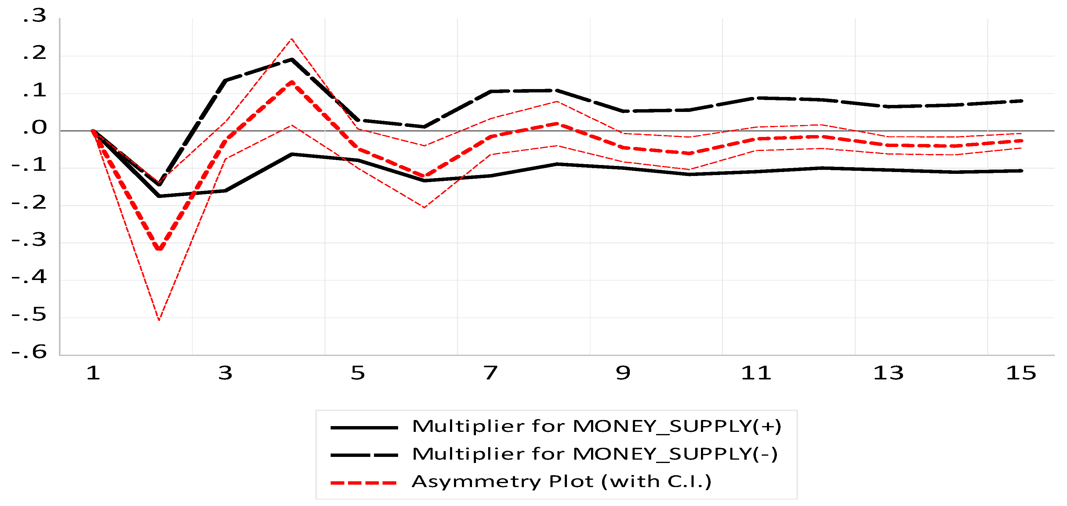
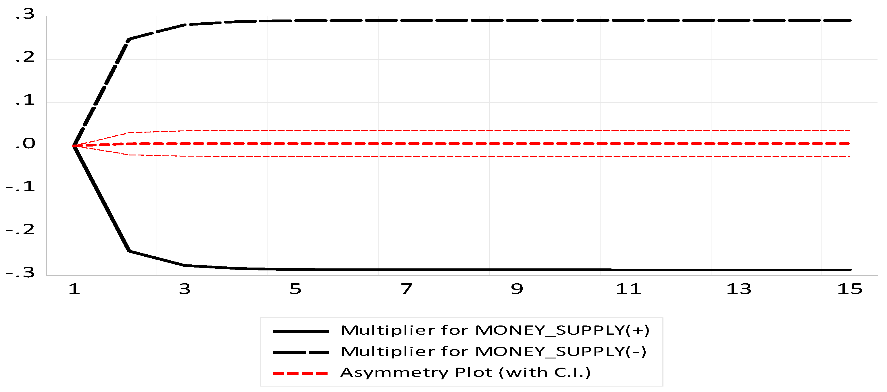
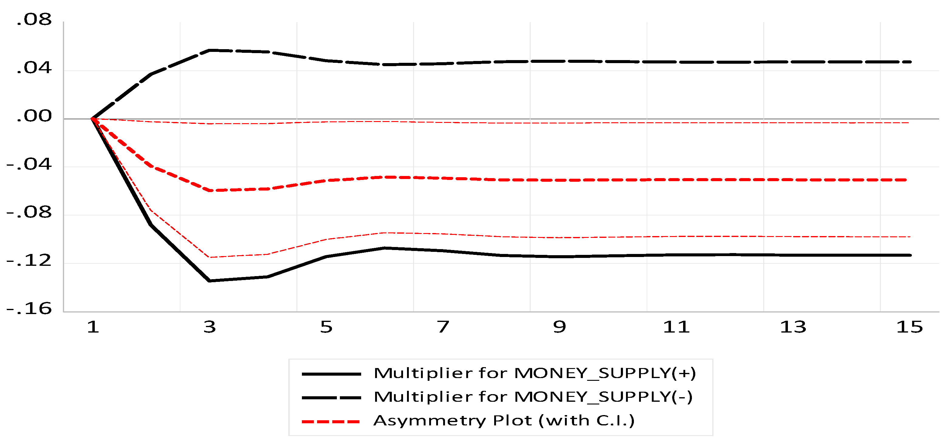
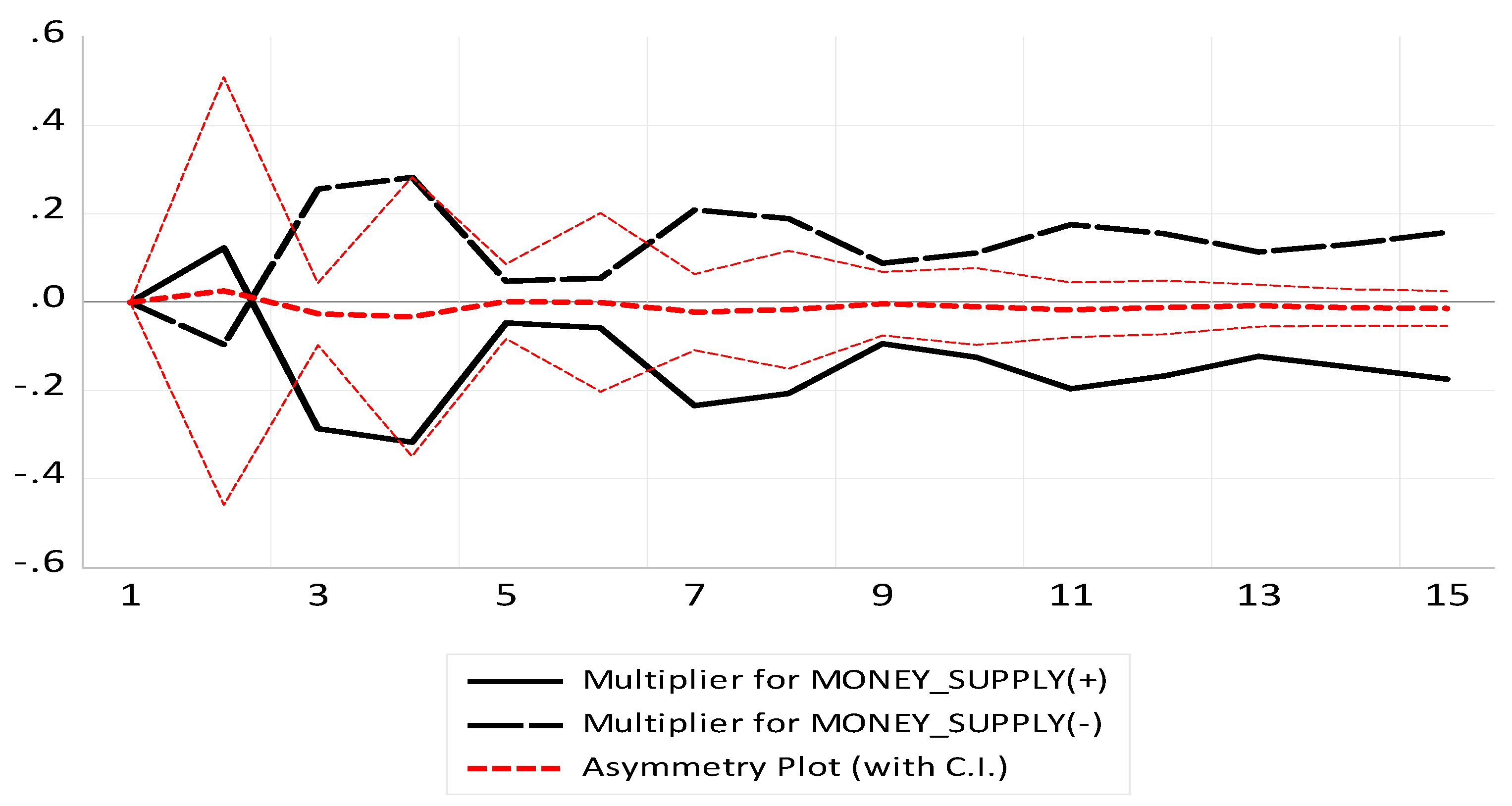
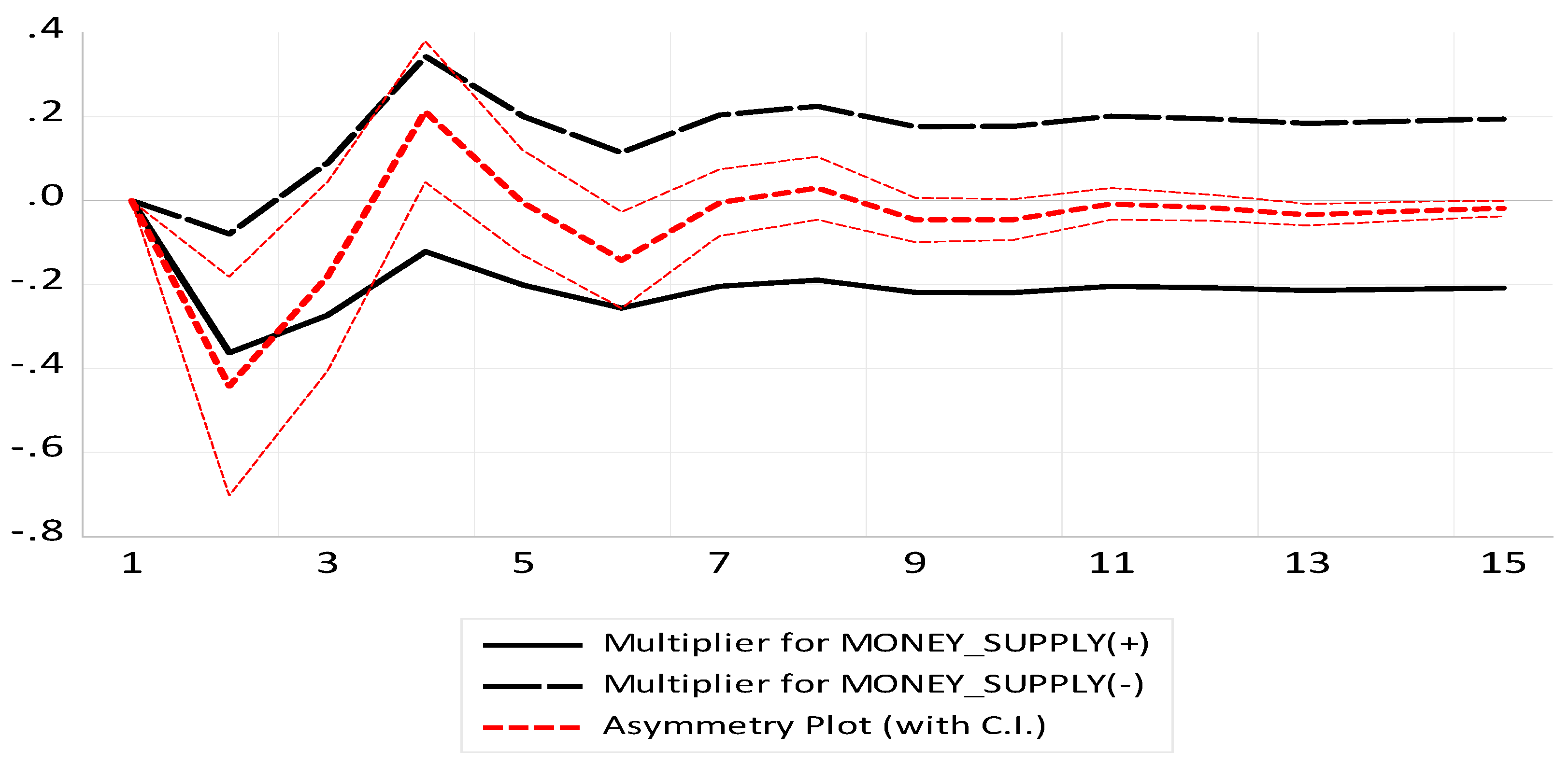
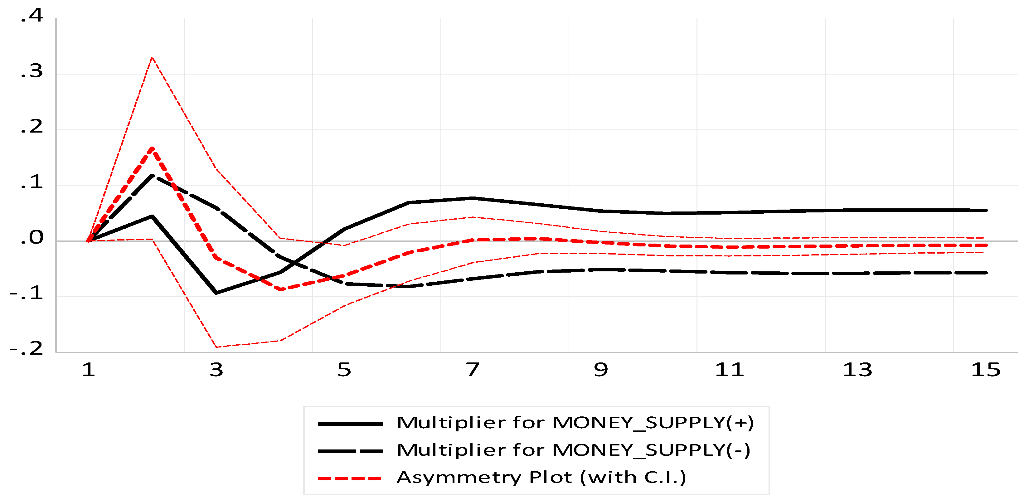
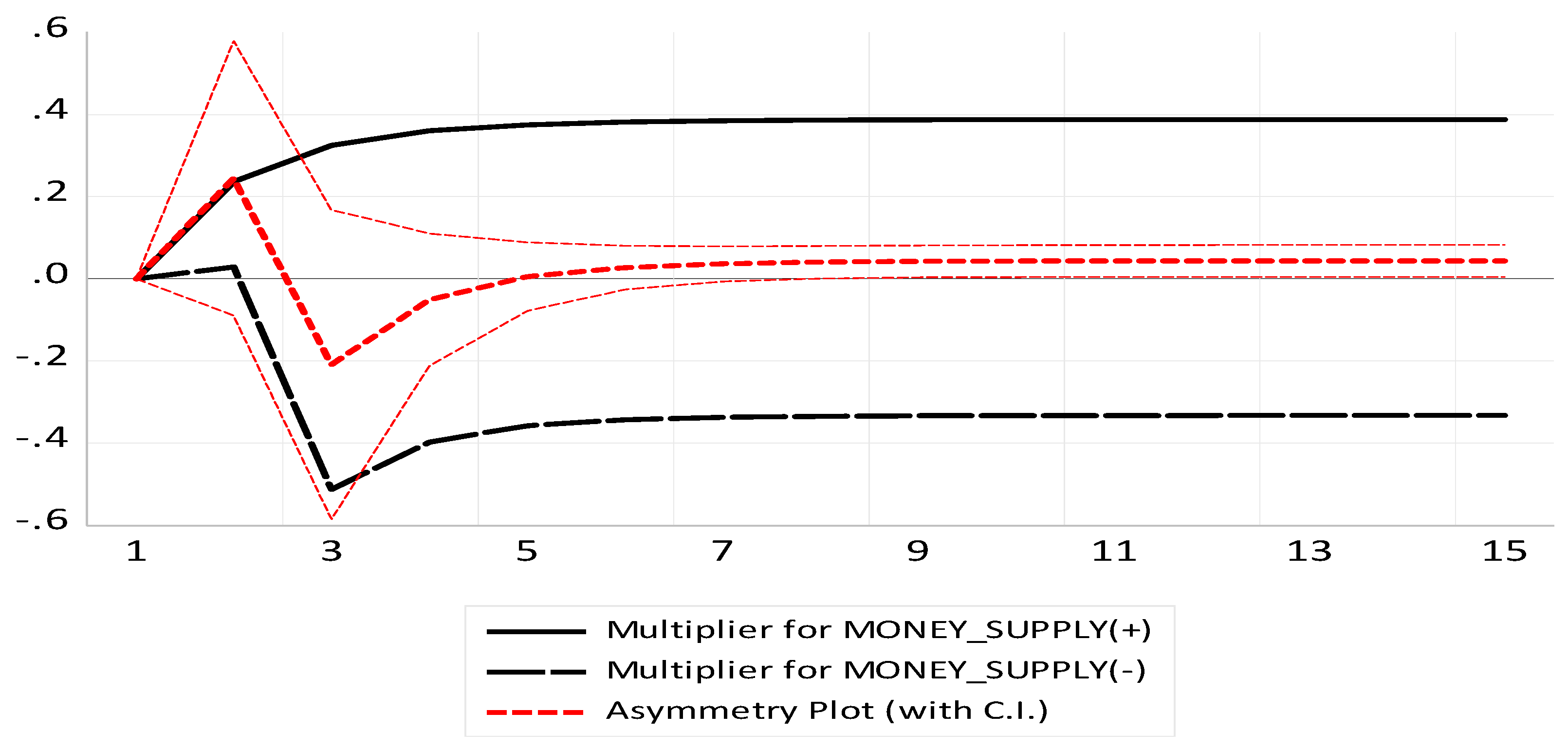
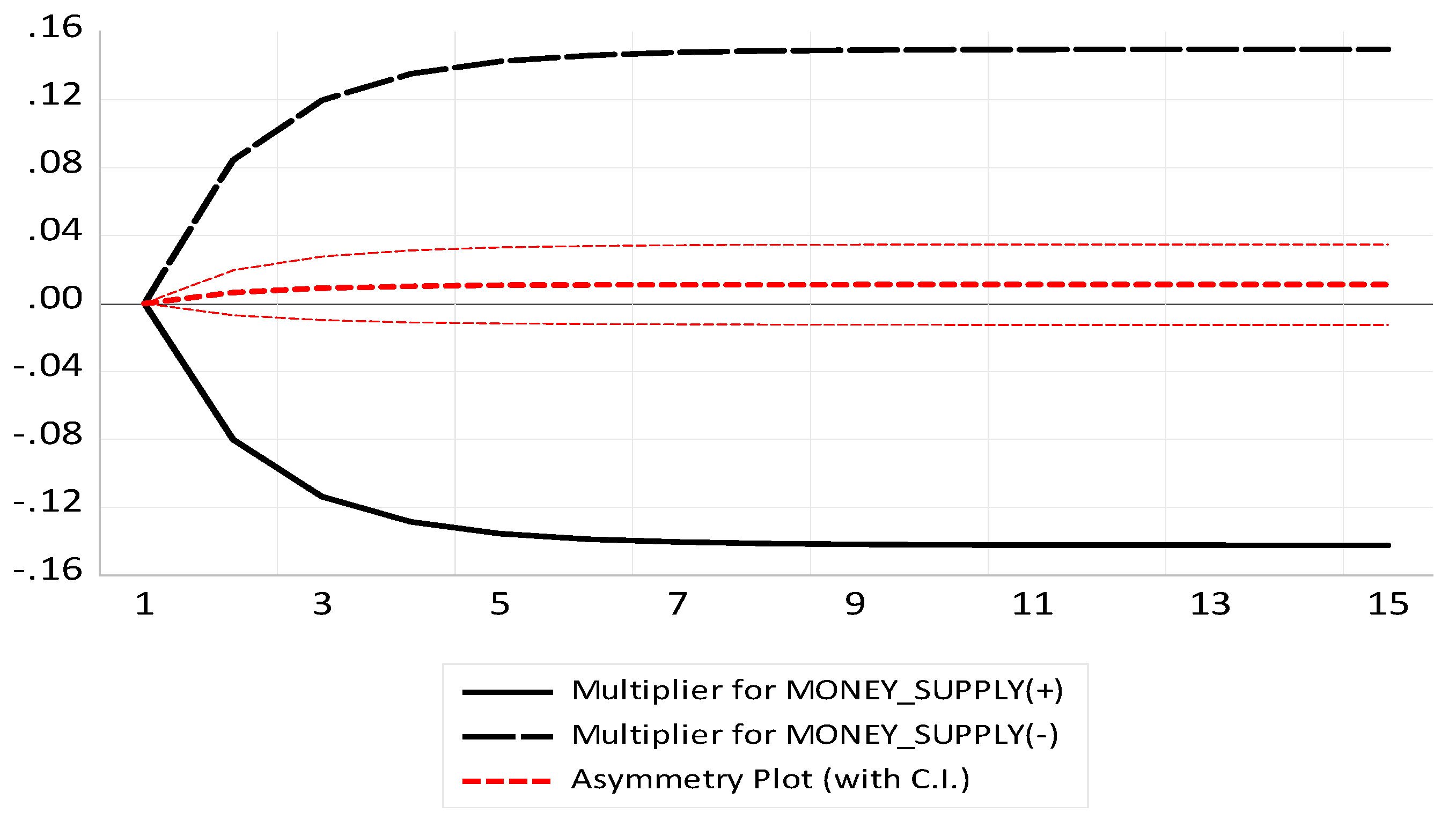
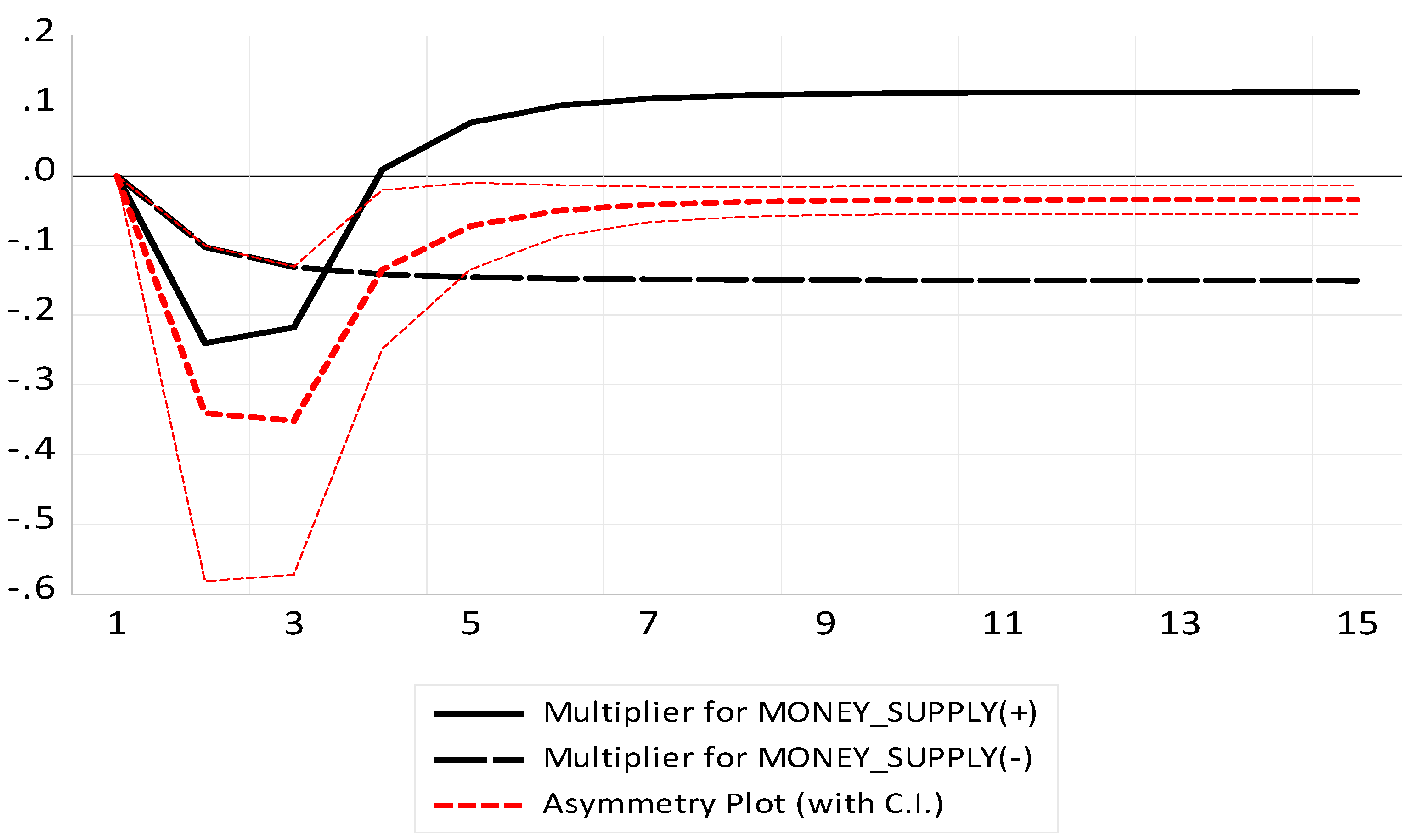
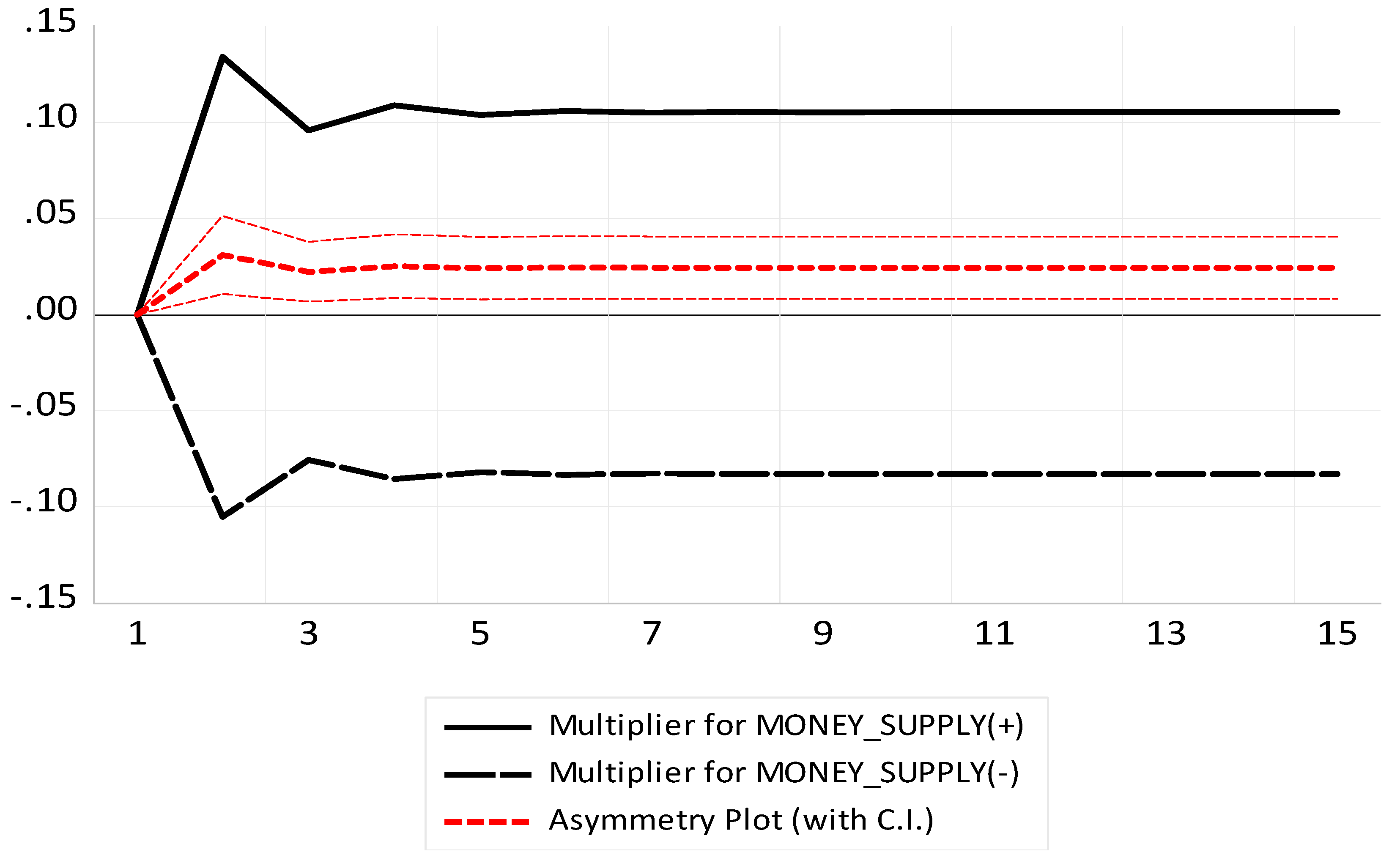
4.6. Dynamic Multiplier Graphs

The dynamic multiplier graphs show the path through which the dependent variables adjust to negative and positive changes in money supply. The dotted black line represents the response to positive changes, whereas the solid black line represents the response to negative changes in money supply. The figures below depict the responses of each sector on the negative and positive shocks in money supply.
The alcoholic beverages and tobacco sector respond negatively to both negative and positive shocks in the short run, until after the second quarter, where the response of the dependent variable is indirect for both positive shocks and negative shocks. Figure 1 further shows that the asymmetry plot in the short run is far from zero, while in the long run, it reverts to around zero. This implies that no asymmetry is detected in the short run, whereas in the long run, the effect of money supply is more asymmetric.
The clothing and footwear sector responds negatively to positive shocks and positively to negative shocks, as shown in Figure 2 below. The effect of the shocks is constant in both the short run and long run, and the magnitude of the response is the same, i.e., around 3, for both negative and positive shocks. The asymmetry plot also conveys more asymmetry for the effect of money supply on the clothing and footwear sector.
Figure 3 visualise that response of the communication sector is more elastic on negative shocks (around −12) than positive shocks (around 4). This is backed by the asymmetry plot which falls below zero (negative quadrant). Moreover Figure 3 shows that monetary policy shocks has the higher effect in short run than in the long run on this sector.
As portrayed in Figure 4 positive shocks in money supply results in an instant increase on prices in the education sector, while negative shocks decrease prices in the same sector in the long run. After the second quarter, the opposite is the case. The magnitude of the response is the same, suggesting that there is asymmetry in the effect of money supply in the education sector.
The effects of both positive and negative shocks in money supply results in an immediate reduction in prices in the health sector. However, Figure 5 further shows that in the long run, negative shocks result in an increase in prices; on the other hand, positive shocks result in a decrease in prices. The magnitude of the response is the same in the long run.
Monetary policy shocks have a higher effect on the households’ contents and equipment sector in the short run than in the long run. The short-term effect in this sector is characterised by a lack of asymmetry, which is denoted by an asymmetry plot variation that is far from zero. However, in the long run, asymmetry is present. As manifested below in Figure 6.
Figure 7 reveals that the response of the housing and utilities sector to negative shocks is not instantaneous, as it takes more than two quarters for it to respond, whereas the response to positive shocks is rapid. The magnitude of the effect is more or less the same, particularly in the long run.
While Figure 8 reveals that, monetary policy shocks have a smaller effect on the recreation and culture sector in the short run; however, over time, it also appears that the effect increases with the same magnitude for both negative and positive shocks.
In the short run, monetary policy shocks result in a price reduction in the restaurants and hotels sector. However, it also appears in Figure 9 that after the third quarter, positive shocks result in an increase in the price levels in this sector. Over time, the magnitude from negative and positive shocks becomes stable, and the asymmetry plot is around zero.
Figure 10 below reveals that the transport sector is more elastic towards positive shocks in money supply in the short run. It takes two quarters for the effect to become stable. These findings of dynamic multipliers coincide with that of the ECM, which revealed that the speed of adjustment is very fast in most sectors.
Holistically, the dynamic multiplier graphs for each model show that the adjustment of the dependent variables from positive and negative shocks varies across sectors. This supports what was postulated by Imbs et al. (2011), i.e., that responsiveness is not the same across economic activities—it depends on each sector’s vulnerability to shocks.

5. Conclusions

Based on the findings, this study concludes that there is a non-linear effect of money supply on sectoral inflation only in the long run, although this effect is sector specific. There are discrepancies in sectoral responses, and for that reason, aggregate inflation may not be a good indicator of the inflation path in South Africa, as it may underestimate sectoral variations. The changes in monetary policy (contractional and expansional) pushes inflation in most sectors in opposite directions, which renders the QTM invalid in the case of South African data. This study recommends that monetary authorities in South Africa (SARB) should consider the use of sectoral inflation to reflect the success of its monetary policy (IT) and mitigate discrepancies in sectoral responses through the application of the diverse monetary strategy, which will help to stabilise inflation across sectors. The policy implications and practicality of these findings is that in South Africa, aggregate inflation does not reflect the true inflation paths. Furthermore, this study recommends that monetary authorities ought to consider sector-based targets to eliminate heterogeneity among sectors. Although this study uncovers several intriguing findings, as with any analysis of this nature, it also raises many questions for future research. One prospective future research paper could examine the sources of heterogeneity in the responsiveness of inflation across sectors. The last potential area of research is to evaluate the effectiveness of monetary policy in ensuring price stability across economic activities.

Author Contributions

Conceptualization, S.M.; methodology, S.M.; software, S.M.; validation, D.D.T. and K.D.I.; formal analysis, S.M.; investigation, S.M.; resources, S.M.; data curation, S.M.; writing—original draft preparation, S.M. and K.DI.; writing—review and editing, K.D.I. and S.M.; visualization, S.M.; supervision, K.D.I. and D.D.T.; project administration, K.D.I. All authors have read and agreed to the published version of the manuscript.

Funding

This study was funded by the National Research Fund (NRF), fund reference number: MND190717456808.

Data Availability Statement

Data is available on request through authors’ direct contacts, under some terms and conditions.

Conflicts of Interest

The authors declare no conflict of interest.

Appendix A. CUSUM Test Graphs for Each Model

1. 
Clothing and footwear sector
Economies 11 00071 i001
2. 
Communication sector
Economies 11 00071 i002
3. 
Education sector
Economies 11 00071 i003
4. 
Food and non-alcoholic beverages sector
Economies 11 00071 i004
5. 
Health sector
Economies 11 00071 i005
6. 
Households’ contents and equipment sector
Economies 11 00071 i006
7. 
Housing and utilities sector
Economies 11 00071 i007
8. 
Recreation and culture sector
Economies 11 00071 i008
9. 
Restaurants and Hotels
Economies 11 00071 i009
10. 
Transport sector
Economies 11 00071 i010

Appendix B. Summary of Diagnostic Tests

TestsResults
Alcoholic beverages and tobacco sector
Heteroskedasticity Test: Breusch–Pagan–Godfrey  Prob. 0.0515 > 0.05
Serial Correlation LM Test: Breusch–Godfrey    Prob. 0.5973 > 0.05
Normality test: Jarque–Bera    Prob. 0.5538 > 0.05
Model specification: Ramsey RESET Test    Prob. 0.1696 > 0.05
Stability: CUSUM testSignificant at 5%
Clothing and footwear sector
Heteroskedasticity Test: Breusch–Pagan–Godfrey    Prob. 0.6138 > 0.05
Serial Correlation LM Test: Breusch–Godfrey    Prob. 0.8313 > 0.05
Normality test: Jarque–Bera    Prob. 0.4287 > 0.05
Model specification: Ramsey RESET Test    Prob. 0.1299 > 0.05
Stability: CUSUM testSignificant at 5%, but not for CUCUM SQ
Communication sector
Heteroskedasticity Test: Breusch–Pagan–Godfrey    Prob. 0.7166 > 0.05
Serial Correlation LM Test: Breusch–Godfrey    Prob. 0.3826 > 0.05
Normality test: Jarque–Bera    Prob. 0.6249 > 0.05
Model specification: Ramsey RESET Test    Prob. 0.2436 > 0.05
Stability: CUSUM testSignificant at 5%
Education sector
Heteroskedasticity Test: Breusch–Pagan–Godfrey    Prob. 0.3268 > 0.05
Serial Correlation LM Test: Breusch–Godfrey    Prob. 0.1302 > 0.05
Normality test: Jarque–Bera    Prob. 0.5666 > 0.05
Model specification: Ramsey RESET Test    Prob. 0.6320 > 0.05
Stability: CUSUM testSignificant at 5%
Health sector
Heteroskedasticity Test: Breusch–Pagan–Godfrey    Prob. 0.2266 > 0.05
Serial Correlation LM Test: Breusch–Godfrey    Prob. 0.1258 > 0.05
Normality test: Jarque–Bera    Prob. 0.1301 > 0.05
Model specification: Ramsey RESET Test    Prob. 0.1688 > 0.05
Stability: CUSUM testSignificant at 5%
Households’ contents and equipment sector
Heteroskedasticity Test: Breusch–Pagan–Godfrey    Prob. 0.0853 > 0.05
Serial Correlation LM Test: Breusch–Godfrey    Prob. 0.0946 > 0.05
Normality test: Jarque–Bera    Prob. 0.0966 > 0.05
Model specification: Ramsey RESET Test    Prob. 0.4399 > 0.05
Stability: CUSUM testSignificant at 5%, but not for CUCUM SQ
Housing and utilities sector
Heteroskedasticity Test: Breusch–Pagan–Godfrey    Prob. 0.1451 > 0.05
Serial Correlation LM Test: Breusch–Godfrey    Prob. 0.2266 > 0.05
Normality test: Jarque–Bera    Prob. 0.1491 > 0.05
Model specification: Ramsey RESET Test    Prob. 0.1496 > 0.05
Stability: CUSUM testSignificant at 5%
Recreation and culture sector
Heteroskedasticity Test: Breusch–Pagan–Godfrey    Prob. 0.4303 > 0.05
Serial Correlation LM Test: Breusch–Godfrey    Prob. 0.3315 > 0.05
Normality test: Jarque–Bera    Prob. 0.1473 > 0.05
Model specification: Ramsey RESET Test    Prob. 0.1637 > 0.05
Stability: CUSUM testSignificant at 5%
Restaurants and hotels sector
Heteroskedasticity Test: Breusch–Pagan–Godfrey    Prob. 0.2758 > 0.05
Serial Correlation LM Test: Breusch–Godfrey    Prob. 0.6136 > 0.05
Normality test: Jarque–Bera    Prob. 0.2893 > 0.05
Model specification: Ramsey RESET Test    Prob. 0.5468 > 0.05
Stability: CUSUM testSignificant at 5%, but not for CUCUM SQ
Transport sector
Heteroskedasticity Test: Breusch–Pagan–Godfrey    Prob. 0.0946 > 0.05
Serial Correlation LM Test: Breusch–Godfrey    Prob. 0.7490 > 0.05
Normality test: Jarque–Bera    Prob. 0.9291 > 0.05
Model specification: Ramsey RESET Test    Prob. 0.8915 > 0.05
Stability: CUSUM testSignificant at 5%
Source: compiled by the authors from the estimation results.

References

  1. Abate, Tadesse Wudu. 2020. Macro-economic Determinants of Recent Inflation in Ethiopia. Journal of World Economic Research 9: 136–42. [Google Scholar] [CrossRef]
  2. Abdelsalam, Mamdouh Abdelmoula M. 2018. Asymmetric Effect of Monetary Policy in Emerging Countries: The Case of Egypt. Applied Economics and Finance 5: 1–11. [Google Scholar] [CrossRef] [Green Version]
  3. Adusei, Micheael. 2013. Is Inflation in South Africa a Structural or Monetary Phenomenon? British Journal of Economics, Management and Trade 3: 60–72. [Google Scholar] [CrossRef]
  4. Agenor, Pierre Richard. 2001. Asymmetric Effect of Monetary Policy Shocks. Washington, DC: World Bank Working Paper 20433. [Google Scholar]
  5. Akinboade, Oludele Akiloye, Franz Krige Siebrits, and Elizabeth Wambach Niedermeier. 2004. The Determinants of Inflation in South Africa: An Econometric Analysis. Nairobi: AERC. [Google Scholar]
  6. Alehegn, Mebtu Melaku. 2021. Determinants of inflationin Sub-Saharan Africa: A systematic Review. Horn of Africa Journal of Business and Economics (HAJBE) 4: 17–23. [Google Scholar]
  7. Alemu, Minyahil, Wondaferahu Mulugeta, and Yikal Wassie. 2016. Monetary Policy and Inflation Dynamics in Ethiopia: An Empirical Analysis. Global Journal of Human Social Science: Economics 16: 44–60. [Google Scholar]
  8. Amassoma, Ditimi, Krey Sunday, and Emma Ebere Onyedikachi. 2018. The influence of money supply on inflation in Nigeria. Journao of Economics ana Management 31: 5–23. [Google Scholar] [CrossRef]
  9. Atil, Assia, and Mourad Saouli. 2020. Determinants of Inflation in Algeria: Analysis with a Vector Error Correction Model from 2001 to 2016. ASJP 7: 429–44. [Google Scholar]
  10. Atkin, Tim, and G. La Cava. 2017. The Transmission of Monetary Policy: How Does It Work? RBA Bulletin-September 2017. Available online: https://www.rba.gov.au/publications/bulletin/2017/sep/1.html (accessed on 12 October 2022).
  11. Badokhon, Sultana, and Faisal Rana. 2021. Macroeconomic determinants of inflation in middle east and north african countries. Palarch’s Journal of Archaeology of Egypt/Egoptology 18: 151–67. [Google Scholar]
  12. Bellemare, Charles, Rolande Kpekou Tossou, and Kevin Moran. 2020. The Determinents of Consumer Expectation: Evidence from US and Canada. No. 2020-52. Ottawa: Bank of Canada Staff Working Paper. [Google Scholar]
  13. Caglayan, Ebru, and Melek Asta. 2012. Interest Reaction Function of the Central Bank: The Case of Czech Republic. International Journal of Business and Social Sciences 3: 225–32. [Google Scholar]
  14. Cao, Tang. 2015. Paradox of Inflation: The Study on Correlation between Money Supply and Inflation in New Era. Ann Arbor: Arizona State University. [Google Scholar]
  15. Chaudhary, Sunil Kumar, and Li Xiumin. 2018. Analysis of the Determinants of Inflation in Nepal. American Journal of Economics 8: 209–12. [Google Scholar]
  16. Cooray, Arusha, and Naceur Khraief. 2018. Money growth and inflation: New evidence from a nonlinear and asymetric analysis. The Manchester School 87: 543–77. [Google Scholar] [CrossRef]
  17. Cukierman, Alex, and Antol Muscatell. 2008. Nonlinear Taylor Rules and Asymmetric Preferences in Central Banking: Evidence from the United Kingdom and the United. The B.E Journal of Macroeconomics 8. [Google Scholar] [CrossRef]
  18. Dajcman, Silvo. 2020. Nonlinear effects of monetary policy on the consumer loans market. Enomic Computationand Economic Cybernetics Studies and Research 54. [Google Scholar] [CrossRef]
  19. De Grauwe, Paul, and Magdalena Polan. 2005. Is Inflation Always and Everywhere a Monetary Phenomenon? Scandinaviana Journal of Economics 107: 239–59. [Google Scholar] [CrossRef]
  20. De Sá, Rodrigo, and Marcelo S. Portugal. 2015. Central bank and asymmetric preferences: An application of sieve estimators to the U.S. and Brazil. Economic Modelling 51: 72–83. [Google Scholar] [CrossRef] [Green Version]
  21. Debortoli, Davide, Ario Forni, Luca Gambetti, and Luca Sala. 2017. Asymmetric Effects of Monetary Policy Easing and Tightening. CEPR Discussion Paper No. DP15005. Available online: https://papers.ssrn.com/sol3/papers.cfm?abstract_id=3650120 (accessed on 14 November 2022).
  22. Ditimi, Amasoma, Keji Sunday, and Emma Ebere Onyedikachi. 2017. The Upshot of Money Supply and Inflation in Nigeria. Valahian Journal of Economic Studies 8: 75–90. [Google Scholar] [CrossRef] [Green Version]
  23. Dolado, Juan J., Maria Dolores, and Ruge Murcia. 2004. Are Central Banks Reaction Functions Asymmetric?: Evidence from Some Central Banks. Madrid: Department of Economics, Universidad Carlos lll de Madrid. [Google Scholar]
  24. Dua, Pami, and Deepika Goel. 2021. Determinants of Inflation in India. The Journal of Developing Areas 55: 205–21. [Google Scholar] [CrossRef]
  25. Espinosa-Vega, Marco A. 1997. How Powerful Is Monetary Policy in the Long Run? Economic Review-Federal reserve bank of Atlanta 83: 12. [Google Scholar]
  26. Esumanba, Sampon Vivian, Nanaa Danaa, and Eria Akyaa Konadu. 2019. The I mpact of Money Supply on Inflation Rate in Ghana. Research Journal of Finance and Accounting 10: 156–70. [Google Scholar]
  27. Friedman, Milton. 1989. Quantity theory of money. In Money. London: Palgrave Macmillian, pp. 1–40. [Google Scholar]
  28. Imbs, Jean, Eric Jondeau, and Florian Pelgrin. 2011. Sectoral Phillips Curves and the Aggregate Phillips curve. Journal of Monetary Economics 58: 328–44. [Google Scholar] [CrossRef]
  29. Jawadi, Reji, Shushanta K. Mallick, and Ricardo M. Sousa. 2013. Nonlinear Monetary Policy Reaction Functions in Large Emerging Economies: The Case of Brazil and China. Applied Economics 46: 973–84. [Google Scholar] [CrossRef]
  30. Katria, Sagar, Niaz Ahmed Bhutto, Flahhuddin Butt, Azhar Ali Domki, and Hyder Ali Khawaja. 2011. Is There Any Tradeoff Between Inflation And Unemployment? The Case of SAARC Countries. Pakistan Journal of ccommerce and Social science 8: 867–86. [Google Scholar]
  31. Kemal, Ali M. 2006. Is Inflation In Pakistan Monetary Phenomenon? The Pakista Development Review 45: 213–20. [Google Scholar]
  32. Kiganda, Evans. 2014. Relationship between money supply and inflation in Kenya. Journal of Social Economics 2: 63–83. [Google Scholar]
  33. Kisswani, Khalid, and Mohammad I. Elian. 2017. Exploring the nexus between oil prices and sectoral stock prices: Nonlinear evidence from Kuwait stock exchange. Cngent Economics and Finance 5: 1286061. [Google Scholar] [CrossRef]
  34. Komijani, Akbar, Mostafa Sargolzaei, Razieh Ahmad, and Marzieh Ahmadi. 2012. Asymmetric Effects of Monetary Shocks on Growth and Inflation: Case study in Iran. International Journal of Business and Social Science 3: 224–30. [Google Scholar]
  35. Kumar, Ankit, and Pradyumna Dash. 2020. Changing transmission of monetary policy on disaggregate inflation in India. Economic Modelling 92: 109–25. [Google Scholar] [CrossRef]
  36. Loayza, Norman, and Raimundo Soto. 2002. Inflation Targeting: An Overview. Series on Central Banking, Analysis, and Economic Policies, No. 5. Washington, DC: World Bank. [Google Scholar]
  37. Loungani, Prakash, and Phillip Swagel. 2001. Sources of Inflation in Developing Countries. (December 2001). IMF Working Paper No.01/198. Available online: https://ssrn.com/abstract=880326 (accessed on 14 September 2022).
  38. Mahyar, Hami. 2017. The Effect of Inflation on Financial Development Indicators in Iran (2000–2015). Studies in Business and Economics 12: 53–62. [Google Scholar]
  39. Murayama, Haruhiko. 2017. Why Does Money Supply Growth Not Push Up Prices? Chuo City: Tokyo Research Institute Economic Report, Summer. Available online: https://www.kyotobank.co.jp/houjin/report/pdf/201708_02_e.pdf (accessed on 14 September 2022).
  40. Narayan, Paresh Kumar, and Ruipeng Liu. 2015. A unit root model for trending time series energy variables. Energy Economies 50: 391–402. [Google Scholar] [CrossRef]
  41. Nelson, Edward. 2008. Why Money Growth Determines Inflation in the Long Run: Answering the Woodford Critique. Journal of Money, Credit and Banking 40: 1791–814. [Google Scholar] [CrossRef]
  42. Nobay, Robert A., and David A. Peel. 2003. Optimal Monetary Policy in a Model of Asymmetric Bank Preferences. The Economic Journal 113: 657–65. [Google Scholar] [CrossRef]
  43. Ofori, Collins Frimpong, Benjamin Adjei Danquah, and Xuegong Zhang. 2017. The Impact of Money Supply on Inflation, A Case of Ghana. Imperial Journal of Interdisciplinary Research 3: 2312–18. [Google Scholar]
  44. Perasan, M. Hashem, Yongcheol Shin, and Richard J. Smith. 2001. Bounds testing approaches to the analysis of level relationship. Journal of Applied Econometrics 16: 289–326. [Google Scholar]
  45. Perevalov, Nikita, and Philip Maier. 2010. On the Advantages of Disaggregated Data: Insights from Forecasting the U.S. Economy in a Data-Rich Enviromnent. No. 2010-10. Ottawa: Bank of Canada. [Google Scholar]
  46. Rasool, Horoon, and Md. Tarique. 2017. Determinants of Inflation: Evidence from India using Autoregressive Distributed Lagged Approach. Asian Journal of Research in Banking and Finance 8: 1–17. [Google Scholar] [CrossRef]
  47. Roshan, Sedigheh Atrkar. 2014. Inflation and Money supply growth in Iran: Empirical Evidences from Cointegration and Causality. Iranian Economic Review 18: 131–52. [Google Scholar]
  48. Shin, Yongcheol, Byungvhul Yu, and Matthew Greenwood Nimmo. 2014. Modelling Asymmetric Cointegration and Dynamic Multipliers in a Nonlinear ARDL Framework. New York: Festschrift in Honor of Peter Schmidt Springer, pp. 281–314. [Google Scholar]
  49. Statistics South Africa. 2021. The Annual Reweighted and Industry Based Consumer Price Index of December; Pretoria: Statistics South Africa.
  50. Sultana, Nair, Rabiunnesa Koli, and Mahamuda Firoj. 2019. Causal relationship of money supply and inflation: A study of bangladesh. Asian Economic and Financial Review 9: 42–51. [Google Scholar] [CrossRef] [Green Version]
  51. Taslim, Mohammad Ali. 1982. Inflation in Bangladesh: A Reexamination of the Structuralist, and Monetarist Controversy. The Bangladesh Development Studies, 23–52. Available online: https://www.jstor.org/stable/4094338 (accessed on 14 September 2022).
  52. Tolulope, Olumuyiwa. 2016. Asymmetry Effects of Monetary Policy Shocks on Output in Nigeria: A Non-Linear Autoregressive Distributed Lag (ARDL) Approach. Available online: https://www.researchgate.net/publication/320907736 (accessed on 14 September 2022).
  53. Uddin, Ijaz. 2020. What determine inflation in Pakistan: An investigation through structural Equation modeling by using time series data for a period from 1975 to 2017. Economic Consultant 4: 54–72. [Google Scholar] [CrossRef]
  54. Ullah, Sana, Iihan Ozturk, and Sidra Sohail. 2021. The asymmetric effects of fiscal and monetary policy instruments on Pakistan’s envirinmental Pollution. Enviromnental Science and Pollution Research 28: 7450–61. [Google Scholar] [CrossRef] [PubMed]
  55. Wang, X. 2017. The Quantity Theory of Money: An Empirical and Quantitative Rassessment. Available online: htttps://sites.wustl.edu/xiwang/files/2017/09/QTMmainCIA-v206pt.pdf (accessed on 14 September 2022).
Figure 1. Dynamic multiplier for the alcoholic beverages and tobacco sector.
Economies 11 00071 g001
Figure 2. Dynamic multiplier for the clothing and footwear sector.
Economies 11 00071 g002
Figure 3. Dynamic multiplier for the communication sector.
Economies 11 00071 g003
Figure 4. Dynamic multiplier for the education sector.
Economies 11 00071 g004
Figure 5. Dynamic multiplier for the health sector.
Economies 11 00071 g005
Figure 6. Dynamic multiplier for the households’ contents and equipment sector.
Economies 11 00071 g006
Figure 7. Dynamic multiplier for the housing and utilities sector.
Economies 11 00071 g007
Figure 8. Dynamic multiplier for the recreation and culture sector.
Economies 11 00071 g008
Figure 9. Dynamic multiplier for the restaurants and hotels sector.
Economies 11 00071 g009
Figure 10. Dynamic multiplier for the transport sector.
Economies 11 00071 g010
Table 1. Consumer price index sectors weights.
Consumer Price Index (CPI) ComponentsComponent’s Percentage Weights in the Basket
1. Housing42.36%
2. Transportation18.18%
3. Food and Beverages14.26%
4. Medical Care8.49%
5. Education and Communication6.41%
6. Recreation 5.11%
7. Other Goods and services2.74%
8. Apparel2.46%
Source: Authors’ compilation from the data extracted from, Statistics South Africa (2021).
Table 2. List of variables in the model.
Independent Variables and DescriptionUnitsSourceExpected Sign
1. Money supply
M 3 t
%Easy Data+
2. Oil price
O P t
%Easy Data+
Dependent Variables (Sectoral inflation)
P t
1. Food and non-alcoholic beverages%Easy Data+
2. Alcoholic beverages and tobacco%Easy Data+
3. Clothing and Footwear%Easy Data+
4. Housing and utilities%Easy Data+
5. Households’ contents and equipment%Easy Data+
6. Health%Easy Data+
7. Transport%Easy Data+
8. Communication%Easy Data+
9. Recreation and culture%Easy Data+
10. Education%Easy Data+
11. Restaurants and hotels%Easy Data+
12. Miscellaneous goods and services%Easy Data+
Source: compiled by the authors based on data collected from Easy Data.
Table 3. Unit root results: ADF.
Critical Values
VariablesTau Stat1%5%10%Order
Money supply−9.79484−4.08887−3.47255−3.16345I (1)
Oil price−7.89026−2.59574−1.94513−1.61398I (0)
Sectoral inflation
Alcoholic beverages and tobacco−19.0511−4.88713−3.47255−3.16345I (1)
Clothing and Footwear−6.91878−2.59574−1.94513−1.61398I (0)
Communication−5.54312−4.08335−3.47003−3.16198I (0)
Education−7.56257−3.52423−2.90235−2.58858I (1)
Food and non-alcoholic beverages−4.93840−3.51905−2.90013−2.58740I (0)
Health−6.80065−3.52423−2.90235−2.58858I (1)
Households’ contents and equipment−4.83999−4.08335−3.47003−3.16198I (0)
Housing and utilities−3.96782−3.53320−2.90621−2.59062I (0)
Miscellaneous goods and services−4.97819−3.52423−2.90235−2.58858I (1)
Recreation and culture−5.23732−4.08335−3.47003−3.16198I (0)
Restaurants and hotels−5.21867−4.14458−3.49869−3.17857I (0)
Transport−8.64064−2.59574−1.94513−1.61398I (0)
Source: compiled by the authors from the estimation results.
Table 4. Cointegration test results.
Lower Bound I (0)Upper Bound I (0)
Dependent VariablesF Stat1%2.5%5%10%1%2.5%5%10%
Alcoholic beverages and tobacco11.786012.723.233.694.293.774.354.895.61
Clothing and Footwear8.4109772.723.233.694.293.774.354.895.61
Communication7.8130472.723.233.694.293.774.354.895.61
Education5.9830432.723.233.694.293.774.354.895.61
Food and non-alcoholic beverages2.600832.723.233.694.293.774.354.895.61
Health8.1197892.723.233.694.293.774.354.895.61
Households’ contents and equipment7.1873142.723.233.694.293.774.354.895.61
Housing and utilities5.1354562.723.233.694.293.774.354.895.61
Miscellaneous goods and services1.8288202.723.233.694.293.774.354.895.61
Recreation and culture96.330652.723.233.694.293.774.354.895.61
Restaurants and hotels14.259502.723.233.694.293.774.354.895.61
Transport63.879612.723.233.694.293.774.354.895.61
Source: compiled by the authors from the estimation results.
Table 5. NARDL short-term results.
INDEPENDENT VARIABLEALCOHOLIC
BEVERAGES
AND
TOBACCO
CLOTHING
AND
FOOTWEAR
COMMUNICATIONEDUCATIONHEALTHHOUSEHOLDS
CONTENTS
AND
EQUIPMENTS
HOUSING
AND
UTILITIES
RECREATION
AND
CULTURE
RESTAURANTS
AND
HOTELS
TRANSPORT
constant6.27 [0.0000]−0.04 [0.9293]−0.20 [0.1848]1.14 [0.0190]3.03 [0.0000]0.62 [0.0009]0.24 [0.5472]−0.12 [0.5957]1.64 [0.0079]0.15 [0.6892]
Δ (S (−1))0.77 [0.00205] −0.04 [0.3529]−0.31 [0.0247]0.06 [0.3100]0.36 [0.0020]0.04 [0.1274]
Δ ( M 3 t + ) −0.01 [0.817]0.04 [0.4820]
Δ ( M 3 t ) −0.02 [0.7644] −0.11 [0.0872]
Δ ( O P t ) 0.005 [0.3081] −0.00 [0.1952] 0.00 [0.8639]
Δ ( M 3 t + ( 1 ) ) −0.15 [0.0122]
Δ ( M 3 t ( 1 ) ) 0.18 [0.0379]
Δ ( O P t ( 1 ) ) 0.01 [0.0083] −0.00 [0.6230]
ECM (−1)−2.35 [0.0000]−0.86 [0.0000]−1.01 [0.0000]−0.50 [0.0074]−1.40 [0.0000]−0.58 [0.0000]−0.31 [0.0016]−0.53 [0.0000]−0.67 [0.0000]−1.01 [0.0000]
Source: compiled by the authors from the estimation results.
Table 6. Long-term relations.
M 3 t + M 3 t O P t
SectorsCoefficientsCoefficientsCoefficients
Alcoholic beverages and tobacco−0.11 [0.0000]−0.08 [0.0005]−0.01 [0.0064]
Clothing and Footwear−0.28 [0.0914]−0.29 [0.0701]−0.00 [0.6074]
Communication−0.00 [0.9009]−0.00 [0.9578]0.00 [0.7045]
Education−0.13 [0.1308]−0.12 [0.1626]−0.02 [0.1106]
Health−0.20 [0.0000]−0.17 [0.0000]−0.02 [0.0066]
Households’ contents and equipment0.05 [0.5351]0.06 [0.4423]−0.00 [0.2323]
Housing and utilities0.44 [0.2874]0.41 [0.2961]0.06 [0.4856]
Recreation and culture−0.10 [0.4417]−0.12 [0.3510]−0.02 [0.1361]
Restaurants and hotels−0.25 [0.0360]−0.21 [0.0785]−0.00 [0.7263]
Transport0.09 [0.3918]0.07 [0.4870]0.09 [0.0000]
Note: Figures in [ ] represent the probabilities for the respective coefficient. Source: compiled by the authors from the estimation results.
Table 7. Long-term and short-term asymmetry—Wald test.
M 3 t + = M 3 t
(Long Run Asymmetry)
Δ ( M 3 t + ) = Δ ( M 3 t )
(Short Run Asymmetry)
Conclusion
SectorsF StatisticF Statistic
Alcoholic beverages and tobacco5.72 [0.0196]--Long run asymmetry
Clothing and Footwear3.15 [0.0798]--Long run asymmetry
Communication0.00 [0.9224]--Long run symmetry
Education0.90 [0.3442]--Long run symmetry
Health14.04 [0.0004]--Long run asymmetry
Households’ contents and equipment3.33 [0.0724]--Long run asymmetry
Housing and utilities1.14 [0.2883]--Long run symmetry
Recreation and culture0.55 [0.4591]--Long run symmetry
Restaurants and hotels4.25 [0.446]--Long run symmetry
Transport0.04 [0.8307]--Long run symmetry
Source: compiled by the authors from the estimation results.
Table 8. Granger causality test results.
Null HypothesisF-StatisticProbability
Bi-directional causality
Education does not granger cause M3-pos5.165920.0081
M3-pos does not granger cause Education2.599220.0816
Health does not granger cause M3-pos3.418210.0384
M3-pos does not granger cause Health2.540690.0862
Uni-directional causality
Oil price does not granger cause Health2.676500.0758
M3-pos does not granger cause Households’ contents and equipment3.203500.0467
M3-neg does not granger cause Households’ contents and equipment3.338850.0413
M3-pos does not granger cause Housing and utilities2.884240.0627
M3-neg does not granger cause Housing and utilities3.001910.0562
Oil price does not granger cause Recreation and culture3.984950.0230
M3-pos does not granger cause Restaurants and hotels4.991510.0109
M3-neg does not granger cause Restaurants and hotels5.131200.0097
Oil price does not granger cause Transport6.548240.0025
Source: compiled by the author from the estimation results.
Disclaimer/Publisher’s Note: The statements, opinions and data contained in all publications are solely those of the individual author(s) and contributor(s) and not of MDPI and/or the editor(s). MDPI and/or the editor(s) disclaim responsibility for any injury to people or property resulting from any ideas, methods, instructions or products referred to in the content.

