Article

The Twin Impacts of Income Inequality and Unemployment on Murder Crime in African Emerging Economies: A Mixed Models Approach

by
Lindokuhle Talent Zungu
* and
Thamsanqa Reginald Mtshengu
Department of Economics, Faculty of Commerce, Administration and Law, University of Zululand, Kwadlangezwa 3886, South Africa
*
Author to whom correspondence should be addressed.
Economies 2023, 11(2), 58; https://doi.org/10.3390/economies11020058
Submission received: 25 November 2022 / Revised: 1 February 2023 / Accepted: 3 February 2023 / Published: 8 February 2023

Abstract

:
This study analyses the dynamic impact of income inequality and unemployment on crime in a panel of 15 African countries during the period 1994–2019 using four models: the panel vector autoregression model, the generalized method of moments model, the fixed-effect model, and machine learning. These models were chosen due to their ability to address the dynamics of several entities. The variables employed for empirical investigation include income inequality, unemployment, and crime. Machine learning was adopted to find which socioeconomic issues contribute to crime between the two issues at hand. The results show that income inequality accounts for 64% of crime, making it the biggest contributor to crime. The findings further show that an unexpected shock in inequality and unemployment has a significant positive impact on crime in these countries. Even when pre-tax income held by the top 10% and male unemployment is adopted, the study yields similar results. Educational entertainment through secondary enrolment was found to increase crime, while it was found to decrease crime through tertiary enrolment at the tertiary level. Finally, economic development was found to decrease crime. From a policy perspective, the current study suggests to the government that some policies are more appropriate for addressing concerns about income inequality and unemployment (income policy or fiscal policy). Therefore, more policies targeting the distribution of income are crucial, as that might decrease income inequality while at the same time decreasing crime. In addition, policymakers should focus on addressing structural challenges through the implementation of sound structural reform policies that aim to attract investment consistent with job creation, human development, and growth in African economies.

1. Introduction

Over the past decades, the prevalence of criminal activity in Africa has skyrocketed, becoming a major social problem impeding the region’s development. As economies transition from traditional to contemporary ways of living in order to experience socioeconomic and cultural changes, it is predicted that changes in criminal activities will occur. At the same time, this region is suffering from a high level of unemployment, income inequality, and low growth. This poses a question: Is a worsening labor market a breeding ground for crime? Does having a legitimate job reduce one’s willingness to offend? Does the worsening of income inequality necessarily lead to crime? These basic questions are ubiquitous throughout the developing world, and policymakers must consider first reference theory for help. As mentioned earlier, African countries suffer from a number of issues, such as high levels of unemployment and income inequality, with high crime rates. 
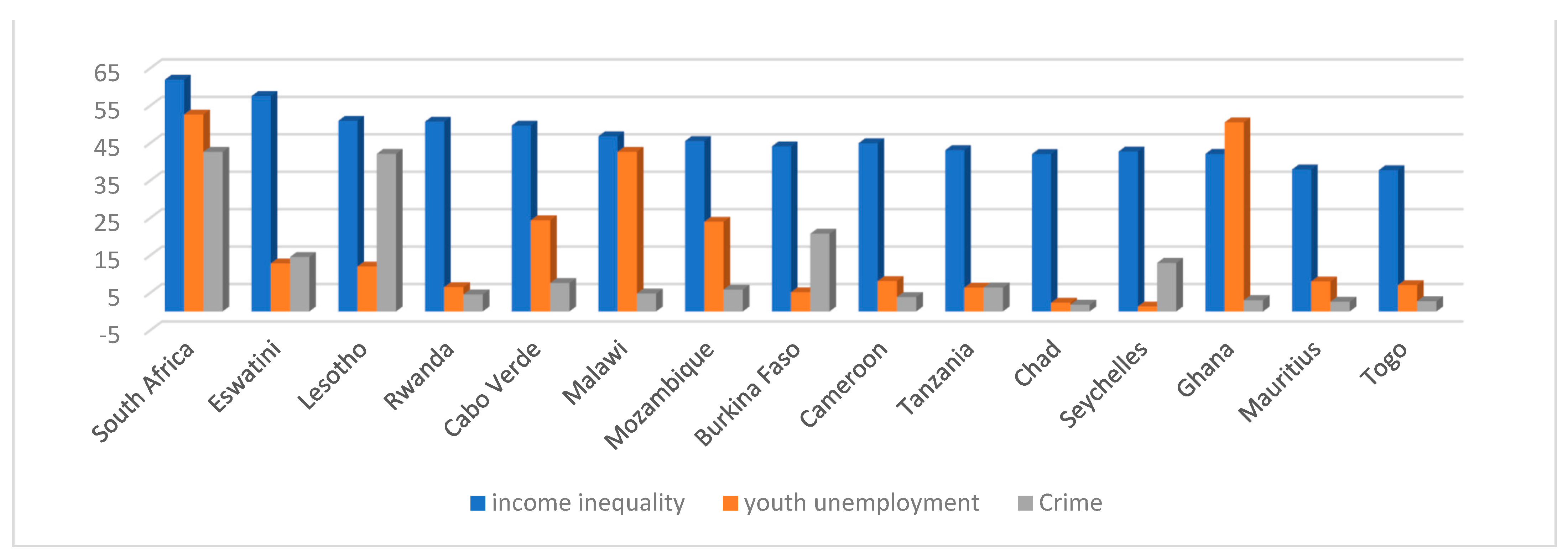
Figure 1 graphically demonstrates the mean Gini coefficient, youth unemployment, and crime covering the period (1994–2019) for 15 African countries.
The graph demonstrates and supports the argument that African countries suffer the most from these global issues, as most countries have a mean Gini coefficient of about 35 points, while the mean of youth unemployment in countries such as South Africa, Malawi, and Ghana is above 35%. In other countries, it is between 10% and 30%, while in others, it is below 10%. The crime rates, especially the murder rate, are high in countries with a high level of income inequality, while they are also high in countries with a high level of youth unemployment. This raises concerns about which socioeconomic issues (income inequality and unemployment) contribute to high crime rates. Are low growth and poor economic development in these countries the drivers of these socioeconomic issues? Finding answers to these questions will help policymakers in African economies to understand the sources of crime in these countries. These studies seek to shed light on the issue by identifying the major contributors to Africa’s crime rate using machine learning (ML).
So far, there has been controversy in both theoretical predictions and empirical research on the impact of unemployment and income inequality on crime. Theories such as the strain hypothesis proposed by Merton (1938) posit that failure to attain material success (usually characterized by a lack of jobs) can frustrate individuals ranking low in the social structure due to economic hardship, thereby breeding retaliatory crime. As a result, a failure by an individual to secure a legitimate job can breed anger, especially when the disadvantaged group finds themselves in the midst of prosperous individuals. This frustration, in turn, may serve as an incentive for economically underprivileged people to commit criminal offenses. After 30 years, Becker (1968), later supported by Ehrlich (1975) in what became known as Becker’s economic theory of crime, viewed this relationship from an economic standpoint, which was profoundly different from the strain theory. Their logic is based on the assumption that individuals tend to commit crimes when the perceived benefits outweigh the penalties.
Furthermore, and more crucially, economists emphasize that unemployment means a lack of genuine work in the labor market. A lack of a legitimate job decreases the opportunity costs of committing a crime, which drives individuals to participate in illegal activity. As a result, economists, unlike sociologists, think unemployment correlates positively with crime. A further contribution to this matter is found in the criminologists’ school of thought, which holds the view that unemployment negatively correlates with crime. They argue that unemployment implies fewer crime victims and fewer stolen products (Felson and Cohen 1980; Cantor and Land 1985, 2001). Precisely, when unemployment rises, the number of individuals from whom criminals may steal decreases; hence, crime is considered a negative consequence of unemployment. They also say unemployment provides additional protection since unemployed individuals spend more time safely indoors and caring for their property. However, the present literature contradicts whether unemployment and income inequality directly or indirectly affect crime. The existing literature is vast and contains numerous conflicting results, with some studies finding the strain theory and Becker’s economic theory of crime appropriate (Fajnzylber et al. 2002; Lobonţ et al. 2017; Costantini et al. 2018; Mazorodze 2020; Kujala et al. 2019; Ayhan and Bursa 2019; Siwach 2018; Anser et al. 2020; Goh and Law 2021), while others leaned more towards the criminologists’ view (Felson and Cohen 1980; Cantor and Land 1985, 2001; Anwar et al. 2017; Zaman 2018), and yet others find inconclusive results (Maddah 2013).
The current study contributes to the existing body of knowledge on the issue. Following the work documented by Mazorodze (2020), the emphasis was on southern African provinces, notably KwaZulu-Natal. He used local municipality-level data observed from 2006–2017 to support the argument that unemployment leads to crime. Our study seeks to extend Mazorodze’s (2020) argument by considering the impact of income inequality on the system; it has become evident from the literature that income inequality may be correlated with crime. Furthermore, we want to include educational and age-dependency variables because they are thought to be highly correlated with crime rates, just like in his study. In a nutshell, we aim to examine the crime response to shock in these variables in African countries.
The current study aims to fill a gap in the literature by incorporating and examining the impact of income inequality and unemployment on educational and age-dependence variables and their effects on crime in African emerging markets, which most previous studies have ignored, as well as by determining the measure contributor of crime between income inequality and unemployment in these countries. The goal of this study is to shed light on an ongoing debate in the literature by building a balanced panel data set of 15 African emerging markets from 1994 to 2019, using the panel vector autoregressive (PVAR) technique as well as the panel generalized method of moments (GMM), fixed-effect (FE) estimators, and machine learning (ML). The PVAR will test the following hypotheses: (1) crime does not respond to a shock of income inequality; (2) crime does not respond to a shock of unemployment in these countries. The ML will be utilized to test the following hypotheses: (3) unemployment is the main contributor to crime in these countries.
A PVAR model for these economies is created based on the variety of measured flaws. Instead of focusing on a single object, this model allows us to investigate the complex interaction of numerous items simultaneously. This study, for example, examined the interactions that occurred between the 15 countries we picked due to their significant commerce. The panel VAR models that handle the dynamics of several entities considered simultaneously are critical for this sort of research. These techniques are generally more comprehensive than ordinary VAR models since they not only analyze variable relationships intuitively, as a standard VAR model but also include a cross-sub-sectional structure. Therefore, this enables us to distinguish between common and specific components, whether in terms of nations, variables, time periods, and so on, and then use this structural knowledge to improve estimation accuracy. It becomes significantly more resilient when dealing with data of varying quality and often of short duration. Static panel techniques or interaction effects do not explain these traits. Ultimately, the reason for conducting this research was not a lack of research investigating the effect of income inequality and unemployment on crime within those countries but rather the fact that this correlation may differ significantly from that published in the literature due to differences in the smoothness of industrial prosperity as well as macroeconomic policies executed.
The remainder of the paper is arranged as follows: Section 2 briefly reviews the literature on the issue, while Section 3 provides an outline of the model. Section 4 analyzes the PVAR, GMM, FE, and machine learning outcomes, while Section 5 gives concluding remarks and explores policy implications.

2. Theoretical Framework

2.1. Theoretical Channels of Income Inequality, Unemployment, and Crime

The theoretical foundation of this study is centered around the principles proposed by Becker (1968) and follows the formulation of Freeman (1999) and Edmark (2005). The model assumes that individuals face a choice between engaging in crime or working to get an income. Therefore, this assumption rules out the possibility of combining both activities. The wage from a legitimate job is indicated by W , while the wage sourced from criminal activities is indicated by W b . The model further captures the presence of the idiosyncratic psychological cost ( c ) of engaging in crime, which can be positive or negative, assuming that it is independent and continuously distributed over the population. The rational choice of crime satisfies the following condition:
c   = E ( W b ) E ( W ) .  
This condition simply prevails if the expected returns from crime are higher than the expected returns from legitimate work when the psychological cost is removed. Then, Equation (1) expands to properly define the expected return from crime as follows:
E ( W b ) = ( 1 p ) W b + p ( W b S ) ,  
where p denotes the probability of being caught while engaging in criminal activity and S denotes the cost of the sentence, which includes, among other things, a low standard of living in person, a fine, a reduction in reputation, and restrictions on future employments. The expected income from a legitimate job takes this form:
E ( W ) = ( 1 u ) W + u A ,  
In Equation (3), u depicts the unemployment rate, or the likelihood of being unemployed, whereas A represents the unemployment benefit. In condition 1, substituting Equation (3) for Equation (2) results in the following inequality:
c < [ ( 1 p ) W b + p ( W b S ) ] [ ( 1 u ) W + u A ]
According to Equation (4), an individual chooses to commit a crime rather than work honestly if the psychological cost of a crime c is less than the quantity on the right-hand side. Furthermore, it aids in eliciting the influence of model parameters on the aggregate supply of crime (Edmark 2005): the higher the right-hand side of Equation (4), the greater the likelihood for individuals to commit crimes, with an effect on the aggregate supply of crime. Therefore, Freeman (1999) and Edmark (2005) formulated three assumptions where:
Assumption 1. 
Stipulated that when  W > A  and  u < 1   ( b o t h   v a l i d   a s s u m p t i o n s ) , this implies that the right-hand side of Equation (4) is increasing by    u  since the quantity  [ ( 1 u ) W + u A ]    moves down as  u    increases.
Assumption 2. 
Assume that the people most inclined to commit crimes are unskilled employees.  W  is likely to be far lower than the population’s average pays.
Assumption 3. 
Stipulates that  W b  depends proportionally on the income of higher paid ( H ) : employees, where  W b = v H  with  v < 1 , and the cost of sentence  ( S )  is proportional to the legal earning of the criminal:  S = q W , with  q < 1 .
Therefore, the right-hand side of Equation (4) will be written as:
[ ( 1 p ) v H + p ( v H q W ) ] [ ( 1 u ) W + u A ]  
W s p = H W defines the increasing earning inequality in Equation (5), which implies that the high incentive to do crime is driven by the higher income inequality. Equation (5) increases even when low- and high-paid workers’ incomes rise by a similar percentage. Relative Equation (5) is a decreasing function in c , p and A , while the u and W s p are an increasing function. Therefore, the supply function of crime ( C s ) is introduced to the above key variables as:
C s ( W s p + , p , A + , u + , c )  
Equation (6) derives the general effect these variables may have on crime in a general equilibrium setting. As noted by Edmark (2005), high demand for crime is associated with high levels of income generally. In a nutshell, this refers to the region, not a person. Increasing the income of a region makes it attractive for criminality (thieves, for example), but increasing the income of a person does not cause him to steal, as one might understand. When contrasted with the supply function, this effect is exerted in the opposite direction.
The aggregate demand for crime C d can then be written as
C d ( W + )  
Relatively, Equation (7) has implications for the effect of income on crime. A rise in W (and hence a decrease in income disparity) has a positive influence on demand but a negative effect on supply for a given H . Again, an increase in unemployment has an uncertain final effect on crime. In a nutshell, a decrease in aggregate income may be due to high unemployment, and if the impact on H is lower than that of W , there will be a decrease in demand and an increase in the supply of crime. When Equations (6) and (7) are combined, they will produce the following equation:
  ( 1 ) C * ( W s p ? , p , A , u ? , c )  
where C * is the quantity of crime that causes supply and demand to be equal. The question mark above income inequality and unemployment rate indicates that the sign of these variables cannot be determined a priori. As a result, empirically, two outcomes are possible:
C * ( W s p , p , A , u ? , c )  
C * ( W s p + , p , A , u ? , c + )  
If (9) holds true, the demand effect outweighs the supply effect, and income inequality and unemployment both show a negative sign. When (10) is present, on the other hand, the reverse is true. Even though our theoretical explanation is not directly connected to murder crime, it will be included in this study. This is because, as Grogger (2006) argues, theoretical frameworks of property crime may be utilized to explain economically motivated offenses committed with violence. Furthermore, Kelly (2000) and Edmark (2005) contend that unemployment and income disparity might have an impact on violent crime.

2.2. Empirical Literature

After scrutinizing the empirical literature on this subject, we found that existing studies build on three strands: The Merton strain theory, Becker’s economic theory of crime (Fajnzylber et al. 2002; Lobonţ et al. 2017; Costantini et al. 2018; Mazorodze 2020; Kujala et al. 2019; Ayhan and Bursa 2019; Siwach 2018; Ngozi and Abdul 2020; Anser et al. 2020; Goh and Law 2021), and Shaw and McKay’s social disintegration theory (Felson and Cohen 1980; Cantor and Land 1985, 2001; Anwar et al. 2017; Zaman 2018).
Going as far back as Fajnzylber et al. (2002), they investigated the causality relationship between income inequality and violent crime in a cross-country analysis from 1965 to 1995. Their findings show that income inequality is positively related to crime rates (within each country and, particularly, between countries), and it appears that this correlation reflects causation from income inequality to crime rates, even when controlling for other crime determinants. A decade later, Maddah (2013) studied the same subject as Fajnzylber et al. (2002). However, the author included unemployment in the equations, seeking to find whether income inequality or unemployment is strongly related to the crime rate. He estimated structural VAR and co-integration approaches in Iran covering 1979–2007. His findings contradict each other as he finds income inequality to have no effect on the crime rate. However, ultimately it was unemployment that was reported as a determinant of violent crime. Further attempts on this subject were made by Lobonţ et al. (2017) for Romania, covering 1990–2014, and Anwar et al. (2017) for Pakistan, 1973–2014. These studies used autoregressive (ARDL distributed lag) bounds, testing to investigate the long- and short-run effects of income inequality and the unemployment crime rate. The findings were contradictory, as the Romanian study found that income inequality and unemployment are both positively related to crime rates in the short- and long-run, whereas the Pakistani study found a negative relationship between these variables.
Costantini et al. (2018) built on previous research on the impact of income inequality and unemployment rates on crime (Maddah 2013; Lobonţ et al. 2017; Anwar et al. 2017). The study by Costantini et al. (2018) used panel data from the US covering 1978–2013, using a non-stationary panel model with a factor structure to study the long-run effect of unemployment and income inequality on crime. The results show that income inequality and unemployment have a positive impact on crime, and the crime-theoretical model fits the long-run relationship well. However, their findings contradict those reported by Anwar et al. (2017). Zaman (2018) took a different approach, surveying a large weighted sample of intellectuals about the crime-poverty nexus and exploring a number of socio-economic factors that are concerned with Pakistan’s high crime rate and poverty incidence, such as income inequality, injustice, unemployment, low spending on education and health, and price hikes. Their findings show income and unemployment to be negatively related to the crime rate when they control for some other socioeconomic indicators, thus supporting the findings of Anwar et al. (2017) in Pakistan but contradicting the findings of Maddah (2013), Lobonţ et al. (2017), and Costantini et al. (2018).
The results documented by these researchers were supported by the findings documented by Mazorodze (2020) for KwaZulu-Natal and Kujala et al. (2019) for Europe. In the study by Mazorodze (2020), the focus was on the southern African provinces, particularly KwaZulu-Natal. He used local municipality-level data observed from 2006–2017 and found a positive relationship between youth unemployment and murder crime. While Kujala et al. (2019) documented that the Gini coefficient, S80/S20 ratio, unemployment, and material deprivation are positively associated with crime in Europe, the study findings documented by Kujala et al. (2019) and others were further supported by Ayhan and Bursa (2019) for a panel of 28 European Union countries from 1993–2016 and Siwach (2018) for New York State covering 2008–2014. The European study used second-generation, co-integration, causality tests, and the panel dynamic least squares (PDLS) method. The finding from the co-integration analysis points out that the causality effect starts from unemployment to crime rates, while the PDLS method reveals a positive relationship. The study conducted in New York State used a 2SLS technique.
The recent literature on this subject further produces contradicting results, as in the study by Anser et al. (2020) using a diversified Panel GMM in a panel of 16 countries from 1990–2014. Their findings support the existing literature that claims income inequality and unemployment rates are increasing factors in crime rates while contradicting those who believe both of these variables are decreasing factors in crime rates. Ngozi and Abdul (2020) used pooled ordinary least squares and different GMM techniques to examine the dynamic impact of income inequality on violent crime in panel data from 38 African countries between 2007 and 2012. The findings show that income inequality is a determinant of violent crime in African countries. Last but not least, Goh and Law (2021) studied the same subject matter in Brazil using a NARDL model. Their results show that, in the long run, reducing income inequality will lead to a decrease in the crime rate with a greater deviation, whereas an increase in income inequality tends to lead to an increase in the crime rate with a lower deviation. Their result supports the literature that believes in a positive relationship between income inequality and crime rates.

3. Research Methods and Data Used for the Study

To fulfill the study’s goal, we used a panel of 15 rising African markets from 1994 to 2019. His research focuses on these nations because they have high rates of violent crime, unemployment, and income inequality. Variables indicated in the literature were used in this investigation. We utilized two variables in our empirical research to quantify income inequality and unemployment. One of the most problematic elements of working on crime-related issues is the fact that crime data is usually measured with inaccuracy due to underreporting, causing the observed data to be an underestimate of the true levels of crime. Fear of victimization and distrust in the police have driven some crime victims to opt not to disclose crimes. Technically, the accuracy of crime statistics is determined by three factors: community desire to report crime cases, police efficacy, and police willingness to record all reported instances. To account for the lack of crime data, we selected murder cases (crime) as a proxy for crime because this sort of crime is not as underreported as other types of violent crime (rape, common assault, burglary at residential premises, and robbery with aggravating circumstances). To assess income inequality, we used the Gini coefficient (INE) and pre-tax national income (TOP10) (Nilsson 2004), whereas to capture unemployment in our study, we used two types of unemployment, namely youth unemployment (YOU) and male unemployment (MUN). This is because, while unemployment may reduce legal returns from work, the proclivity to engage in criminal activities increases. Male unemployment is featured in the literature, which asserts that males are the perpetrators of violent crime on a global scale (UNODC 2019). We adjust for educational factors such as secondary (EDS) enrollment in our model to determine the impact of education on the choice to engage in criminal activities. According to the literature, increasing the ratio of school achievement is projected to lower crime rates (Witt et al. 1998). The age dependency ratio indicator (ADRY) is then used to adjust for the proportion of individuals of working age as well as the percentage of employed persons in relation to the overall population. The high percentage of age dependence is said to have aided crime. We use GDP per capita income (GDPp) to adjust for economic development and growth. Finally, we take into account population growth (EDT). According to the urban scaling theory, the number of crimes committed as a function of a city’s population size may follow a super-linear relationship. The variables came from many sources, including the World Development Indicators, SWIID, and the World Inequality Database. These models were estimated using the Rstudio and Stata15 software packages.
Before a detailed presentation of the PVAR, GMM, and FE, the following section will give a brief explanation of machine learning as it aims to find the variables that have a strong impact on crime between income inequality and unemployment.

3.1. Random Forest Model

Random forest (RF) was first described by Breiman (2001) as a collaborative method for building forecast models. The phrase “forest” means a series of decision trees that act to classify weak individuals who strongly influence the dependent variable. An important task in many econometrician fields is the perdition of a variable response based on the set of variables. In many cases, RF has been used by statisticians to find important predictor variables (Breiman 2004; Biau et al. 2008; Meinshausen 2006; Biau 2012). However, the RF not only aims to make the accurate prediction of the response, but it also aims to identify candidates in a group of variables that are most important in predicting and providing the variable importance measures; variates such as extra trees have been used as a major data-analyses tool employed with achievements in various scientific areas (Geurts et al. 2006) and random forests (Breiman 2001).
The RF is a machine learning algorithm; therefore, the RF is a collection of tree predictors developed firstly by growing the tree by splitting the training data sets at each node according to the value of one from a randomly selected subset of variables using classification and regression tree, which is known as growing phase (seven). Next, randomly select the subset of the learning data sets, which is a training set for growing the tree known as the bootstrap phase. Each tree is expanding to the largest extent possible. The growing phases and the bootstrap require the input of random quantities. These quantities are assumed to be independent among trees and are identically distributed. Hence, each tree can be seen as a sample independent of the collaboration of all tree predictors for a given learning set. For hypothesizing, the occurrence runs through each tree in a forest down to the terminal node, which assigns its class with a maximum amount of votes for presenting the RF with the probabilistic interpretation of the forest assumption.
Δ K = { ( p 1 , , p K ) : K = 1 K p k = 1   a n d   p k 0 }  

3.1.1. Feature Importance

In an RF, feature importance is used as a way of describing how much impact a feature has on the model-making decision. In this study for feature importance, the author will rely on the Gini impurity, which measures the chance that a new variable will be correct when randomly classified. This feature is bound by zero and one where one denotes that it is guaranteed that it will be wrong, while zero simply denotes that it is impossible to be wrong.
The Gini impurity of the node is estimated using this equation:
G ( k ) = i = 1 n P ( i ) × ( 1 P ( i ) )  
In this case, P ( i ) is the probability of the record being assigned to class and i is a predicted category of the random class.

3.1.2. Gini Importance

The Gini importance, in this case, is a total reduction of the Gini impurity that comes from a feature, where it is calculated as a weighted sum of the indifference in Gini impurity among the node and its antecedents. Therefore, it takes this form:
G i m p o r t a n c e ( k ) = i = 1 n ( N × G p a r e n t   ) ( N c h i l d 1 × G c h i l d 1 ) ( N c h i l d 2 × G c h i l d 2 )

3.2. Panel Vector Auto Regression (PVAR) Approach

Prior to actually estimating the PVAR model, we will use the cross-sectional dependency (CD) test, Friedman’s (1937) statistic, Frees’ (1995) test statistic, and the Pedroni cointegration test to rule out the potential of cross-sectional dependence. Panel stationarity is as important in panel data analysis as it is in time series analysis. As a consequence, the Im–Peseran–Shin (Im et al. 2003) test will be employed, and the Harris–Tzavalis (Harris and Tzavalis 1999) test will be used for robustness. In African emerging economies, we employed a balance panel VAR approach to capture the dynamic effect of income disparity and unemployment on crime. We followed Maddah’s (2013) lead and used structural VAR in Iran from 1979 to 2007. Our panel VAR model is a system of equations comprised of two models, each with seven endogenous variables, as stated in Section 3. The general model is as follows:
y i t = α 0 + Γ 1 Y i , t 1 + Γ 2 Y i , t 2 + + Γ p Y i , t p + ε i t   i { 1 , 2 , 3 , , N } ,   t { 1 , 2 , 3 , , T i }
where Y i t is a (7 × 1) vector of endogenous variables for year t and country i , which include the murder cases to measure crime (Crime), income inequality (INE), youth unemployment (YOU), the secondary (EDS) enrolment ratio to capture education, the age dependency ratio indicator (ADR), population growth (EDT), and real per capita gross domestic product (GDPp), α 0 is a (7 × 1) vector of a constant,   Γ 1 , 2 , 3 , ,   p is a (7 × 7) matrix of coefficient estimates, and ε i t is a (7 × 1) vector of system innovations, while i is a cross-sectional identifier, and p is selected though observing the value of the Schwarz Bayesian Criterion (SBC) and Akaike information criterion (AIC), which is the optimal lag length of each variable. PVAR analysis selecting the appropriate lag order is among the first stages which need to be undertaken, both in a moment condition and panel-VAR specification. Therefore, PVAR analysis is reliant upon appropriate lag selection.
This model representation is based on Abrigo and Love’s work (Abrigo and Love 2016).

3.3. Generalized Method of Moments and Fixed-Effect Models

To investigate the relationship between income inequality, unemployment, and crime, we apply the difference generalized method of moments (Difference GMM) (Arellano and Bond 1991; Blundell and Bond 1998) and fixed-effect models (FE). We chose the Difference-GMM because we wanted to address the issue of individual effects. The dependent variable will also be included as a lagged explanatory variable in the GMM estimator. Because this research may suffer from the endogeneity problem, this estimating technique is used. Furthermore, the possibility of multiple causations cannot be ruled out for several of our control variables. Finally, there are two sorts of instruments in the GMM estimator: external and internal. In the literature, it has been suggested that internal instruments are preferable to external instrumentation for the GMM system. This is due to the fact that choosing an external instrument for the GMM is the most difficult task of the estimation. Therefore, internal instruments, such as lag values of regressors, will be the instruments for the data that the researcher is working with. For the current investigation, we use our capabilities to construct instruments domestically. As a result, endogenous variables are instrumented by their lagged values. In a nutshell, this means that the tool for this analysis must originate within the following:
C r i m e i t = μ i + λ t + β 0 INE i t + β 2 Z i t + u i t  
C r i m e i t = μ i + λ t + β 0 YOU i t + β 2 Z i t + u i t
where t = 1 , , T   a n d   i = 1 , , N , indicates the time dimensions and cross-section and the time dimensions of the panel, correspondingly. Whereas λ t and μ i take for the time and fixed individual effects, respectively, correspondingly, Z it is the vector of control variables, and the errors term is denoted by u i t . Equation (15) investigates the influence of income inequality on crime, whereas Equation (16) investigates the impact of unemployment on crime. Under the entire set of random-effects assumptions, the Hausman test will be utilized to choose between FE and random-effects (RE) estimates. The test findings indicate that the RE assumption is rejected; hence, the FE estimations are employed. To prevent biased estimates due to the lack of other significant explanatory factors, we converted Equations (15) and (16) into a dynamic model by including a lagged term of crime based on the static model, as shown in Equations (17) and (18). In this study, the dynamic panel models are estimated using differential GMM:
C r i m e i t = ξ Δ C r i m e i t 1 + Δ α i + Δ λ t + Δ β 0 INE i t + Δ β 2 Z i t + Δ u i t  
C r i m e i t = ξ Δ C r i m e i t 1 + Δ α i + Δ λ t + Δ β 0 YOU i t + Δ β 2 Z i t + Δ u i t  

4. Analysis of Results and Data Analysis

4.1. Data Analysis

For the current study, we conducted two different models to answer different specific objectives of the study. The PVAR was conducted to analyze the dynamic effects of income inequality and unemployment on crime in 15 African economies. The panel S-GMM was adopted to control for endogeneity and to analyze the impact coefficient of the two variables on crime in support of the results generated by our baseline methodology. We began by performing a data examination to better comprehend the data we were working with.
Table 1 displays the descriptive statistics for the various variables, while Table A1 provide the correction metrix. According to descriptive statistics, the average income inequality captured by the Gini coefficient and unemployment captured by youth unemployment in these countries is around 46.48 and 17.17 percent, respectively, while crime is around 10.29 percent. All of the variables are found to be negatively skewed, as reported.
All of the variables, on the other hand, had kurtosis values within the required range of 2 to 3 percent. The alternative normality hypothesis is contradicted by all of these variables, showing that they are not regularly distributed. Because the probability values of the Jarque–Bera tests for all variables are less than 10%, the implications may be owing to country-specific factors, implying rejection of the alternative hypothesis of normal distribution.
To avoid deceptive parameter estimates, researchers then assess stationarity using a panel data stationarity test, exactly as we would for time-series analysis. Im et al. (2003) produced the Im–Pesaran–Shin test, and Harris and Tzavalis devised the Harris–Tzavalis test (Harris and Tzavalis 1999). The panel data stationarity test is summarized in Table 1.
Table 1 shows that, with the exception of YOU and ADS, all variables are non-stationary in levels and stationary after the first differencing. As can be seen, with the exception of the two stated variables, which are I(0), all of the variables employed in this study are I(1).
To validate the variables used in this study, we investigated for cointegration and cross-sectional independence. Table 2 displays the Pedroni cointegration (Pesaran 2004) and cross-sectional dependence (CD) test statistics (Friedman 1937), as well as Frees’ (1995) test data.
The Pedroni cointegration test and the three cross-sectional reliance tests all strongly reject the null hypothesis of no cointegration and cross-sectional reliance in variables. We further adopt the machine learning developed by Breiman (2001), using the random forest (RF) in this study in order to find the variable that has the highest contribution to crime between income inequality and youth unemployment. We believe this will assist policy-makers in understanding the significant contributor of crime in these countries between the two current issues. We set the number of trees within the RF to 2500 in order to make a prediction of the RF more precisely. The results of the RF are reported in Figure 2, while Table 3 translates the results into percentage format. The first chart on the left-hand side, represented by A, reveals mean decrease accuracy (“%incMSE” test), which tests how poorly the model performs without each variable. The second graph on the right-hand side, denoted by B, reveals the nodes (IncNodePurity), which aims to measure how pure the nodes are at the end of the tree without each variable.
Income inequality (INE) under the mean decreases accuracy; looking at its value %IncMSE, which is 61.04, shows that INE is the biggest contributor to the accuracy of predicting crime. While youth unemployment (YOU) is found to be the second contributor, with a mean decrease accuracy of 44.26%, we believe that these results will help policymakers in African countries understand that the main contributor to crime in these countries is the high level of income inequality. Therefore, re-distributional policies are more significant for these countries.

4.2. The Model Instability, Results, and PVAR Interpretations

Lag length selection is a normal approach in a VAR model before predicting a PVAR. To calculate the lag length, the unconstrained PVAR is estimated with all variables in levels and a maximum number of lags of seven, then lowered by re-estimating the model with one lag fewer at a time until zero (Asteriou and Hall 2007). The values of the Akaike information criterion (AIC) and the Schwarz information criterion (SIC), as well as their corresponding autocorrelations, heteroskedasticity, and normality diagnostics, are examined in each of these models, and the model with the shortest lag duration is chosen. Considering Charemza and Deadman’s (1992) guidelines for restricted observations, such as those used in this work, the maximum number of lags was originally set at seven and gradually dropped to two, which met the Gaussian criteria. Table A2 in Appendix A shows the findings for the optimal number of delays. When estimating the panel VAR model using various data transformations, the second lag appears to be more stable and consistent. The models were estimated after the quality of the data was tested. However, we began by testing the model’s stability using autoregressive (AR) roots for all PVAR models. We discovered that no roots were located beyond the unit circle in any channel, indicating that the stability criterion was met, as shown in Figure 3.
We used PVARs to construct the IRFs because they are more effective at assessing dynamic interactions between orthogonalized variables than VAR coefficients. IRFs can give helpful information on the consequences of a shock in one variable while controlling for other factors. As a result, our discussion for all of the variables in the PVAR system is mostly centered on the IRF plots shown in Figure 3, which also show the IRFs for each variable in relation to a one-standard deviation shock in the other variables. Our study aims to explore the dynamic impact of income inequality and unemployment on crime in African countries. The last row of Figure 4 is of particular importance in this investigation. To begin, the dynamic impact of income inequality (INE L1) on crime (Crime L1) in Figure 4a’s last row demonstrates that crime responds positively to an unanticipated 1% shock to INE L1. From period zero to period seven, the INE L1 has an increasing influence on the crime of roughly 50%. This then converges to negative but above the steady-state area before reverting to negative. The results indicate that the INE L1 has a long-term favorable effect on crime based on the impulsive response. The positive reaction to crime may represent the influence of an increase in the amount of property crime in richer block groups when income differences between them and their lowest adjacent block groups grow.
When poorer households look for nearby crime chances, they are more likely to pick places with higher incomes than areas with lower incomes. Our empirical findings back up what has been reported in the empirical literature, including studies by Maddah (2013) for Iran, Lobonţ et al. (2017) for Romania, Costantini et al. (2018) using panel data from the United States, Ngozi and Abdul (2020) using a panel of 38 African countries, and Goh and Law (2021) for Brazil.
We then estimate the second model in finding the dynamic shock of youth unemployment on crime in African countries. In the last row of Figure 4b, a shock of 1% standard deviation to young unemployment (YOU) subsequently had a 10% positive impact on crime from period zero to period six. This then converged to a negative value but remained above the steady-state zone before reverting to the steady-state region. The impulsive reaction indicates that an unexpected shock has a long-term favorable influence on YOU. The possible reason for the positive impact of youth unemployment on crime is related to the fact that being unemployed may make individuals frustrated, which in turn may lead to violent crime, as scholars argue that criminality is an outcome of social interactions. Thus, if the unemployment rate increases, it may create a criminal culture within some groups of society. People who earn low salaries are more prone to conduct property crimes such as burglary since they will make money even if it is illegal. Because money is the major motivator, assault, and robbery are also linked to high unemployment rates. Poverty and a lack of resources exacerbate crime. We also estimate the simultaneous impact of shocks of income inequality and unemployment on crime by including three variables in our model, as shown in Figure A1 in Appendix A. The results of the simultaneous impact of these variables further support the results reported in the baseline model. Furthermore, our findings support the findings reported by Costantini et al. (2018) using panel data from the US, Mazorodze (2020) focusing on the southern African provinces, particularly KwaZulu-Natal, Kujala et al. (2019) for some countries in Europe, Ayhan and Bursa (2019) for a panel of 28 European Union countries; and Siwach (2018) for New York State.
For both models, we control for economic development using GDP per capita (Lgdp_L1), education entertainment such as secondary enrolment (EDS), the age dependency ratio (AGDP), and population growth (EDT), as shown in Figure 3. In both models, we controlled for economic development in the model in order to examine the dynamic impact of income inequality and unemployment on crime. In order to better understand how crime responds to economic development, we controlled for a GDP per capita shock. We find that an unanticipated 1% shock on an Lgdp L1 has a negative effect on crime and that the effect is substantial in both models one and two (Figure 3). From period zero to period seven, the influence of economic progress on crime is around 1%. This then converges to a positive but below steady-state zone before reversing to a steady-state region. The impulsive reaction indicates that an unanticipated shock has a long-term unfavorable influence on the Lgdp L1. Economic theory documents the rationale behind crime’s negative response to increased economic development or growth, arguing that crime should decrease as economic growth and opportunity improve. This is due to the fact that when legal options for generating revenue grow more profitable, the incentive to participate in illicit conduct lessens. Residents may get increasingly involved in legal rather than illicit activities if their economic prospects improve. This was empirically consistent with studies such as that of Chen and Zhong (2020) for Hong Kong.
On the other hand, a discrepancy appeared between these two models based on the impact of education entertainment (EDS) on crime, as we discovered that crime responds positively to an unexpected 1% shock on EDS of about 5% in the income inequality-crime model, while crime responds negatively to an unexpected 1% shock on EDS of about 4% in the unemployment-crime model. This impulsive reaction indicates that an unanticipated shock has a long-run beneficial influence on secondary education enrollment on crime in Model 1 but a short-run impact in Model 2. It further validates that the impact depends on these topical issues (unemployment and income inequality). The economic intuitions behind the negative impact of education entertainment on crime are that a reduction in crime can most often be achieved through increased crime prevention and that education is the most effective form of crime prevention. This demonstrates that higher education levels are associated with a variety of other characteristics that are thought to be positive predictors of less criminal or antisocial behavior. In general, the empirical literature offers two hypotheses for education’s ability to reduce crime and antisocial conduct. The first point is that education has the capacity to change people’s preferences (and, in turn, their breadth of choices). The second explanation is that education influences time preference (understanding the consequences of one’s actions typically induces an individual to postpone the immediate fulfilment of wants). Some scholars claim that education leads to a decreased time preference for current consumption (by teaching one about the possible negative features of quick pleasure) and a higher time preference for future consumption (by teaching one the benefits of working in the present to prepare for the future). This finding supports the results documented by Lochner (2020).
Following a 1% standard deviation shock on age dependence (AGDY L1), both models showed a further positive response to crime. This demonstrates that in the income inequality-crime model, AGDY L1 had a 0.6% positive influence on crime from period zero to period three and 0.7% in the unemployment-crime model from period zero to period four. This then converged to a negative but above the steady-state region before reverting to the steady-state region. The impulse response indicates that an unanticipated shock has a short-run favorable influence on the AGDY L1.
This kind of relationship has been noted since the beginning of criminology. For example, Quetelet ([1831] 1984) found that the proportion of the population involved in crime tends to peak in adolescence or early adulthood and then decline with age. This finding supports the results documented by Bell et al. (2022).
Lastly, a further positive response to crime was documented in both models following a 1% standard deviation shock on population growth (EDT_L1) of about 4% in the income inequality-crime model and about 5% in the unemployment-crime model. The impulse response signifies a long-run positive impact of an unexpected shock of EDT_L1 on crime in the income inequality-crime model, while in the unemployment-crime model, it has a short-run decreasing impact. The possible reason for the positive impact of population growth on crime is related to the fact that as human overpopulation drives resources and basic necessities, such as food and water, to become scarcer, there will be increased competitiveness for these resources, which leads to elevated crime rates due to drug cartels and theft by people in order to survive. According to the urban scaling theory, the number of crimes committed may follow a superlinear relationship as a function of the population size of a city. For example, if the population size increases by 100%, the incidence of crime may increase by 120% (Chang et al. 2018). This finding supports the results documented by Faryad et al. (2017) for 12 municipalities in the city of Tehran and Chang et al. (2018) for a panel of 250 cities in the United States.

4.3. Empirical Results of the Robustness and Sensitivity Analysis Using the GMM and FE Models

For the robustness and sensitivity models, we used the pre-tax national income top 10% from the world inequality database to measure income inequality and the male unemployment rate to capture the unemployment rate. Other variables have the same definition as defined in the baseline methodology. We then adopt a System Generalized Method of Moments (S-GMM) model to make sure that the results are not sensitive to the model used. The Panel Difference GMM was estimated in our model to support the result of the PVAR and further generate the coefficient impact of income inequality and unemployment on crime in African emerging countries. For our Difference GMM, we set the number of lags to one for yearly differences in our yearly data. We further cut our time period to start from 2006–2019 in order to comply with the conditions of the GMM that T should not be greater than N . While for the fixed effect, the time period was the same as the one adopted in the PVAR model. The results of the robustness and sensitivity checks are reported in Table 3 for the S-GMM and FE methodologies.
The results of the S-GMM and FE empirically support the results reported in the baseline methodology of this study. We find a positive relationship between income inequality captured by the pre-tax national income (TOP10) and crime in model III. Similar results were reported in mode IV when we used male unemployment to capture the unemployment rate. Focusing on the S-GMM model, the magnitude of the income inequality-crime is twice that of the coefficient reported in model IV. In model III, the magnitude is 5.80, while in model IV, it is 2.98. These findings signify that the results reported in the baseline methodology are not sensitive to the variable used or the model adopted. Our empirical findings support what has been reported in the empirical literature, like the study by Maddah (2013) for Iran, Lobonţ et al. (2017) for Romania, Costantini et al. (2018) using panel data from the US, Ngozi and Abdul (2020) using a panel of 38 African countries, and Goh and Law (2021) for Brazil. These studies find income inequality to be the increasing factor in crime, while in unemployment-crime, on the other hand, our results support the findings reported by Costantini et al. (2018) using panel data from the US; Mazorodze (2020) focusing on the southern African provinces, particularly KwaZulu-Natal; Kujala et al. (2019) for some countries in Europe; Ayhan and Bursa (2019) for a panel of 28 European Union countries, and Siwach (2018) for New York State.
Table 3. Income Inequality, unemployment, and crime; GMM and FE Model, African Emerging Countries.
VariablesModel III: Income Inequality-Crime Model IV: Unemployment-Crime
S-GMMFES-GMMFE
Pre-tax National Income (TOP10)5.80 ** (1.30)3.30 *** (0.99)
Male Unemployment (MUN) 2.98 *** (0.10)2.00 *** (0.10)
GDP per Capita (GDPp)−4.93 ** (2.10)−2.45 ** (1.00)−3.02 ** (1.98)−2.00 ** (0.87)
School Enrolment, Secondary (EDS)−2.30 ** (1.02)−3.57 *** (0.06)−1.80 ** (0.70)−2.90 *** (0.09)
Age Dependency (AGDY)2.90 ** (0.80)1.50 ** (0.70)3.69 ** (1.40)0.98 ** (0.25)
Population Growth (EDT)1.90 *** (0.04)2.00 ** (1.00)0.80 *** (0.07)1.43 ** (0.60)
AR(1): p-value0.008 0.005
AR(2): p-value0.180 0.139
Hansen: p-value 0.698 0.598
R 2 0.598 0.608
# of obs.210390210390
# of countries15
Note: Dependent variable is the Crime. The numbers in brackets denote the standard errors in brackets obtained by using the cluster-robust and heteroskedasticity-consistent covariance estimator, allowing for error dependency within individual countries. (***), (**) reflect the 1%, 5% levels of significance, respectively. # means number. Source: Author’s illustration based on data UNODC (2019) SWIID (Solt 2020; WDI 2022).
For both models, we control for economic development using GDP per capita (Lgdp_L1), education variables such as secondary (EDS) and tertiary school (EDT) enrolment, and age dependency ratio (AGDP), as shown in Table 3. In both models, we control for economic development; the findings show that a 1% increase in per capita income reduces the level of crime by 4.93% in model III and 3.02 in model IV. These findings are supported by the results generated in the FE model and further support the results reported by the PVAR technique. Our findings are in line with the findings documented by Costantini et al. (2018) using panel data from the US, Ngozi and Abdul (2020) using a panel of 38 African countries, and Goh and Law (2021) for Brazil.
On the other hand, in line with the results documented in the PVAR in the unemployment-crime model, we find that a 1% increase in school enrolment, secondary (EDS), results in a decrease in crime with a magnitude of about 2.30% in model III and 1.80 in model IV. These results were further supported by the results generated by the FE and, in turn, further supported the results reported in the PVAR model (Lochner 2020).
On another side, a positive impact was documented following a 1% increase in age dependency (AGDY_L1) in both models. This shows that crime increases by 2.90 in the income inequality-crime model and by 1.80% in the unemployment-crime model. The results were further supported by the results generated by the FE and, in turn, further supported the results reported in the PVAR model (Bell et al. 2022).
Lastly, a further increase in crime was documented as a result of a 1% increase in population growth, which led to a 1.9% increase in crime across the two models. These findings are in line with our PVAR model, which shows that crime responds positively to an unexpected shock on EDT. The results were further supported by the results produced by the FE model (Faryad et al. 2017; Chang et al. 2018).
The study results were further compared with those produced by other internal and international studies conducted on the subject matter. Table 4 shows the results of the existing literature on the subject matter to compare with the results of this study. Compared with the results documented by Ngozi and Abdul (2020), in Africa, a 1% increase in income inequality leads to a 7.58 percent increase in crime. When compared with current results, their magnitude is high by 2%, which can be the result of the specific countries adopted within Africa. This, however, supports the argument that income inequality has a significant impact on crime.
However, studies on the unemployment-crime equation are related and support the argument derived from Figure 1 of the variable importance, which shows that income inequality is a significant factor in crime, followed by unemployment. The magnitude impact of income inequality on crime is greater than the magnitude impact of unemployment on crime in almost all of these studies.

5. Conclusions

The extant empirical literature is filled with disputes over the impact of income inequality and unemployment on crime in both developed and developing countries. The current study provides a substantial positive relationship between income inequality, unemployment, and crime in African economies. The results reveal that an unanticipated 1% increase in income inequality and youth unemployment has a favorable effect on crime. For robustness and sensitivity, we used multiple measurements of income inequality (pre-tax national income top 10% from the world inequality database), unemployment (male unemployment rate), and even a different approach (S-GMM and FE). Even by these measures, we yield the same results, as we found that when income inequality increases by 1%, crime increases by 5.80%. While on the other hand, a 1% increase in male unemployment results in a 2.98% increase in crime. These findings were further supported by the FE. The findings are theoretically conceivable and in line with previous research on income inequality and crime, such as Maddah (2013) for Iran, Lobonţ et al. (2017) for Romania, Costantini et al. (2018) for the United States, Ngozi and Abdul (2020) for a panel of 38 Africans, and Goh and Law (2021) for Brazil. Moreover, with unemployment-crime, our findings support the findings reported by Costantini et al. (2018) using panel data from the US, Mazorodze (2020) focusing on the southern African provinces, particularly KwaZulu-Natal, Kujala et al. (2019) for some countries in Europe, Ayhan and Bursa (2019) for a panel of 28 European Union countries and Siwach (2018) for New York State.
We then use machine learning to answer the question: which socioeconomic issues between income inequality and unemployment contribute to high crime rates, specifically in African economies? The results pointed to income inequality as the major contributor to high crime in African countries, as we found that it contributes about 61.04% to crime, while unemployment contributes about 44.26% to crime.
We expanded the argument by including educational variables, such as school enrolment at secondary levels in the system. The results show that crime responds negatively to an unexpected 1% shock on school entertainment through enrolment at the secondary y level. This was further supported by the results generated by the S-GMM and FE.
The use of real GDP per capita to measure the quality of life or economic development was included in the conclusion that low growth and poor economic development in these nations are the root causes of these social concerns. The results show that crime responds negatively to an unexpected 1% rise in per capita income (economic development), supporting the importance of raising living standards in these countries, as it has been demonstrated to reduce crime. The findings are theoretically sound and consistent with recent research, such as the Hong Kong study by Chen and Zhong (2020). Population growth was found to increase crime levels in all models. The study extends the argument in this area by controlling for age dependence. In all models, crime responds negatively to an unexpected 1% shock in age dependency. This was further supported by the results generated from the S-GMM and FE models. Similar findings were documented by Galbraith (1998).
From a policy standpoint, the current study informs the government that some measures are more suited to resolving concerns about income inequality and unemployment (income policy or fiscal policy). As a result, additional measures aimed at income distribution are required, as this may reduce economic disparity while also lowering crime rates. We suggest that future research should focus on a comparative study where this region is compared to Europe or other countries with similar characteristics. Furthermore, a study that aims to find the possibility of nonlinearity in the subject will have a significant contribution. Finally, the study that will seek to determine the reliance on policy regulation on this subject is significant. This is due to the fact that Figure 1: “Graphic analysis of the mean Gini-index, youth employment, and crimes, 1994–2019.” From this figure, it is obvious that for individual countries, the dependencies between the studied indicators can have very significant differences.

Author Contributions

Conceptualization, L.T.Z. and T.R.M.; Methodology, L.T.Z.; Software, L.T.Z.; Validation, L.T.Z.; Formal analysis, L.T.Z.; Investigation, L.T.Z.; Data curation, L.T.Z.; Writing—original draft, L.T.Z.; Writing—review & editing, L.T.Z. and T.R.M.; Visualization, L.T.Z. and T.R.M. All authors have read and agreed to the published version of the manuscript.

Funding

This research received no external funding.

Data Availability Statement

Publicly available datasets were analyzed in this study. These data can be found here: [United Nations Office on Drugs Crime (UNODC 2019). Global Study on Homicide. Vienna. Available online: https://www.unodc.org/gsh/ (accessed on 3 January 2022) and World Development Indicators (WDI 2022). World Bank. Washington, DC. Available online: http://data.worldbank.org/data-catalog/world-development-indicators (accessed on 3 January 2022). Further inquiries can be directed to the corresponding author.

Conflicts of Interest

The author declares no conflict of interest.

Appendix A

Table A1. Correlation.
t-StatisticCRIME INE Top10YOU MUNEDS EDT AGDY LGDP
CRIME1.00
INE0.64 (16.42)1.00
TOP100.60 (10.55)0.78 (20.55)1.00
YOU0.22 (4.48)0.15 (3.01)0.30 (2.00)1.00
MUN0.30 (2.66)0.45 (4.78)0.55 (4.61)0.14 (3.01)1.00
EDS0.24 (5.05)0.24 (4.99)0.28 (6.54)0.48 (10.94)0.30 (2.70)1.00
EDT−0.37 (−2.55)−0.27 (3.56)−0.57 (5.00)0.35 (7.43)−0.50 (6.90)0.72 (20.68)1.00
AGDY0.33 (7.04)−0.37 (7.85)−0.38 (4.75)−0.37 (7.84)−0.44 (8.00)−0.86 (33.75)−0.69 (18.84)1.00
LGDP−0.26 (5.44)0.41 (8.95)−0.50 (7.34)0.41 (9.11)−0.56 (7.21)0.88 (37.94)0.65 (16.85)−0.84 (30.72)1.00
Source: Author’s illustration based on SWIID (Solt 2020; WDI 2022).
Table A2. Lag selection-criteria.
LagCDJJ-P.vMBICMAICMQIC
10.99190.220.30−633.07−114.90−310.33
20.99101.340.35−658.40−83.05−230.20
30.9950.200.45−356.62−61.51−110.40
40.9920.700.50−135.09−40.10−80.91
50.9910.220.20−100.91−15.10−59.40
60.99…..
Source: Author’s illustration based on SWIID (Solt 2020; WDI 2022).
Figure A1. Response of crime on a simultaneous shock on income inequality and unemployment. Figure A1 depicts the simultaneous influence of income inequality and unemployment on crime. The results, as can be seen, further support our main hypothesis. The gray regions represent the 95% confidence interval. Furthermore, the IRFs provide two periods: a short run of zero to four years and a lengthy run of five to ten years. As a result, the orthogonalized IRF is interpreted in accordance with the established short-run and long-run periods. Author’s artwork based on SWIID (Solt 2020; WDI 2022).
Economies 11 00058 g0a1

References

  1. Abrigo, Michael, and Inessa Love. 2016. Estimation of panel vector autoregression in Stata. The Stata Journal 16: 778–804. [Google Scholar] [CrossRef]
  2. Anser, Muhammad Khalid, Yousaf Zahid, Nassani Abdelmohsen, Alotaibi Saad, Kabbani Ahmad, and Zaman Khalid. 2020. Dynamic linkages between poverty, inequality, crime, and social expenditures in a panel of 16 countries: Two-step GMM estimates. Economic Structures 9: 43. [Google Scholar] [CrossRef]
  3. Anwar, Awais, Noman Arshed, and Sofia Anwar. 2017. Socio-economic determinants of crime: An empirical study of Pakistan. International Journal of Economics and Financial Issues 7: 312–22. [Google Scholar]
  4. Arellano, Manuel, and Stephen Bond. 1991. Some tests of specification for panel data: Monte Carlo evidence and an application to employment. Review of Economic Studies Limited 58: 277–97. [Google Scholar] [CrossRef]
  5. Asteriou, Dimitris, and Stephen Hall. 2007. Applied Econometrics: A Modern Approach. New York: Palgrave Macmillan. [Google Scholar]
  6. Ayhan, Fatih, and Nurbanu Bursa. 2019. Unemployment and crime nexus in european union countries: A panel data analysis. Journal of Administrative Sciences 17: 465–84. [Google Scholar] [CrossRef]
  7. Becker, Gary. 1968. Crime and punishment: An economic approach. Journal of Political Economy 76: 169–217. [Google Scholar] [CrossRef]
  8. Bell, Brian, Costa Rui, and Machin Stephen. 2022. Why Does Education Reduce Crime? Journal of Political Economy 130: 1. [Google Scholar] [CrossRef]
  9. Biau, Gerard, Devroye Luc, and Lugosi Gabor. 2008. Consistency of random forests and other averaging classifiers. Journal of Machine Learning Research 9: 2015–33. [Google Scholar]
  10. Biau, Gerard. 2012. Analysis of a Random Forests Model. Journal of Machine Learning Research 13: 1063–95. [Google Scholar]
  11. Blundell, Richard, and Stephen Bond. 1998. Initial conditions and moment restrictions in dynamic panel data models. Journal of Econometrics 87: 115–43. [Google Scholar] [CrossRef]
  12. Breiman, Leo. 2001. Random forests. Machine Learning 45: 5–32. [Google Scholar] [CrossRef]
  13. Breiman, Leo. 2004. Consistency for a Simple Model of Random Forests. Technical Report 670. Berkeley: University of California. [Google Scholar]
  14. Cantor, David, and Kenneth Land. 1985. Unemployment and crime rates in the post-World War II United States: A theoretical and empirical analysis. American Sociological Review 50: 317–32. [Google Scholar] [CrossRef]
  15. Cantor, David, and Kenneth Land. 2001. Unemployment and crime rate fluctuations: A comment on Greenberg. Journal of Quantitative Criminology 17: 329–42. [Google Scholar] [CrossRef]
  16. Chang, Yu Sang, Sung Sup Choi, Jinsoo Lee, and Jin Won Chang. 2018. Population size vs. number of crime–Is the relationship super-linear? International Journal of Information and Decision Science 9: 26–39. [Google Scholar] [CrossRef]
  17. Charemza, Wojaciech, and Derek Deadman. 1992. New Directions in Econometric Practice: General to Specific Modelling, Cointegration, and Vector Autoregression. Edited by Edward Elgar. Berkeley: The University of California, p. 370. [Google Scholar]
  18. Chen, Xi, and Hua Zhong. 2020. Development and crime drop: A time-series analysis of crime rates in Hong Kong in the last three decades. International Journal of Offender Therapy and Comparative Criminology, 1–25. [Google Scholar] [CrossRef]
  19. Costantini, Mauro, Meco Iris, and Paradiso Antonion. 2018. Do inequality, unemployment and deterrence affect crime over the long run? Regional Studies 52: 558–71. [Google Scholar] [CrossRef]
  20. Edmark, Karin. 2005. Unemployment and crime: Is there a connection? Scandinavian Journal of Economics 107: 353–73. [Google Scholar] [CrossRef]
  21. Ehrlich, Isaac. 1975. The deterrent effect of capital punishment: A question of life and death. American Economic Review 65: 397–417. [Google Scholar]
  22. Fajnzylber, Pablo, Ledeman Daniel, and Loayza Nnrman. 2002. What causes violent crime? European Economic Review 46: 1323–57. [Google Scholar] [CrossRef]
  23. Faryad, Parhiz, Zarrabi Asghar, and Meshkini Abolfazl. 2017. Analyzing the Relationship between Crime and Population Intensity (12th Municipality Area of Tehran as a Case Study). European Online Journal of Natural and Social Sciences 6: 1. Available online: www.european-science.com (accessed on 3 February 2022).
  24. Felson, Marcus, and Lawrence Cohen. 1980. Human ecology and crime: A routine activity approach. Human Ecology 8: 389–406. [Google Scholar] [CrossRef]
  25. Freeman, Richard. 1999. The economics of crime. Handbook of Labor Economics 3: 3529–71. [Google Scholar] [CrossRef]
  26. Frees, Edward. 1995. Assessing cross-sectional correlation in panel data. Journal of Econometrics 69: 393–414. [Google Scholar] [CrossRef]
  27. Friedman, Milton. 1937. The use of ranks to avoid the assumption of normality implicit in the analysis of variance. Journal of the American Statistical Association 32: 675–701. [Google Scholar] [CrossRef]
  28. Galbraith, James. 1998. Created Unequal: The Crisis in American Pay. New York: Free Press. [Google Scholar]
  29. Geurts, Pierre, Ernst Damien, and Wehenkel Louis. 2006. Extremely randomized trees. Machine Learning 63: 3–42. [Google Scholar] [CrossRef]
  30. Goh, Lim Thye, and Siong Hook Law. 2021. The crime rate and income inequality in Brazil: A nonlinear ARDL approach. International Journal of Economic Policy in Emerging Economies 15: 1. Available online: https://www.inderscienceonline.com/doi/pdf/10.1504/IJEPEE.2022.120063 (accessed on 3 January 2022). [CrossRef]
  31. Grogger, John. 2006. An economic model of recent trends in violence. In The Crime Drop in America, 2nd ed. Edited by A. Blumstein and J. Wallman. Cambridge: Cambridge University Press, pp. 266–87. [Google Scholar]
  32. Harris, Richard, and Elias Tzavalis. 1999. Inference for unit roots in dynamic panels where the time dimension is fixed. Journal of Econometrics 91: 201–26. [Google Scholar] [CrossRef]
  33. Im, Kyung, So Pesaran, M. Hashem, and Shin Yongcheol. 2003. Testing for unit roots in heterogeneous panels. Journal of Econometrics 115: 53–74. [Google Scholar] [CrossRef]
  34. Kelly, Morgan. 2000. Inequality and crime. The Review of Economics and Statistics 82: 530–39. [Google Scholar] [CrossRef]
  35. Kujala, Pietari, Kallio Johanna, and Niemelä Mikko. 2019. Income inequality, poverty, and fear of crime in Europe. SAGE Publications 53: 163–85. [Google Scholar] [CrossRef]
  36. Lobonţ, Oana-Ramona, Nicolescu Ana-Cristina, Moldovan Nicoleta-Claudia, and Kuloğlu Ayhan. 2017. The effect of socioeconomic factors on crime rates in Romania: A macro-level analysis. Economic Research-Ekonomska Istraživanja 30: 91–111. [Google Scholar] [CrossRef]
  37. Lochner, Lance. 2020. Education and crime. In The Economics of Education, 2nd ed. A Comprehensive Overview. chap. 9. Amsterdam: ScienceDirect, pp. 109–17. [Google Scholar] [CrossRef]
  38. Maddah, Majid. 2013. The effect of unemployment and income inequality on crimes, a time series analysis. International Journal of Economics Research 2: 37–42. [Google Scholar]
  39. Mazorodze, Brain Tavonga. 2020. Youth unemployment and murder crimes in KwaZulu-Natal, South Africa. Cogent Economics & Finance 8: 1799480. [Google Scholar] [CrossRef]
  40. Meinshausen, Nicolai. 2006. Quantile regression forests. Journal of Machine Learning Research 7: 983–99. [Google Scholar]
  41. Merton, Robert. 1938. Social structure and anomie. American Sociological Review 3: 672–82. [Google Scholar] [CrossRef]
  42. Ngozi, Adeleye, and Jamal Abdul. 2020. Dynamic analysis of violent crime and income inequality in Africa. International Journal of Economics, Commerce and Management. VIII, p. 2. Available online: http://ijecm.co.uk/ (accessed on 19 January 2022).
  43. Nilsson, Anna. 2004. Income Inequality and Crime: The Case of Sweden. Working Paper. Uppsala: Institute of Labour Market Policy Evaluation, p. 6. [Google Scholar]
  44. Pesaran, Hashen. 2004. General Diagnostic Tests for Cross-Sectional Dependence in Panels. Cambridge Working Papers in Economics No. 0435. Cambridge: Faculty of Economics, The University of Cambridge. [Google Scholar] [CrossRef]
  45. Quetelet, Adolphe. 1984. Research on the Propensity for Crime at Different Ages. Translated by S. Sylvester. Cincinnati: Anderson. First published 1831. [Google Scholar]
  46. Siwach, Garima. 2018. Unemployment shocks for individuals on the margin: Exploring recidivism effects. Labour Economics 52: 231–44. [Google Scholar] [CrossRef]
  47. Solt, Frederick. 2020. The standardized world Income-inequality database. Social Science Quarterly 90: 231–42. [Google Scholar] [CrossRef]
  48. United Nations Office on Drugs Crime UNODC. 2019. Global Study on Homicide. Vienna. Available online: https://www.unodc.org/gsh/ (accessed on 3 January 2022).
  49. Witt, Robert, Clarke Alan, and Fielding Nigel. 1998. Crime, earnings inequality and unemployment in England and Wales. Applied Economics Letters 5: 265–67. [Google Scholar] [CrossRef]
  50. World Development Indicators WDI. 2022. World Bank. Washington, DC. Available online: http://data.worldbank.org/data-catalog/world-development-indicators (accessed on 3 January 2022).
  51. Zaman, Khalid. 2018. Crime-poverty nexus: An intellectual survey. Forensic Res Criminol International Journal 6: 327–29. [Google Scholar] [CrossRef]
Figure 1. Graphic analysis of the mean Gini-index, youth unemployment, and crime, 1994–2019. Source: Author’s illustration based on data UNODC (2019) SWIID (Solt 2020; WDI 2022).
Economies 11 00058 g001
Figure 2. Variable Importance. Note: The left panel (A) shows permutation-based variable importance, and the right panel (B) displays Crime importance for an RF binary classification model developed for the BCW dataset. Source: Author’s illustration based on data UNODC (2019) SWIID (Solt 2020; WDI 2022).
Economies 11 00058 g002
Figure 3. Eigenvalue stability condition. Note: All the eigenvalues lie inside the unit circle. PVAR satisfies stability conditions. Source: Author’s illustration based on data UNODC (2019) SWIID (Solt 2020; WDI 2022).
Economies 11 00058 g003
Figure 4. (a) Crime’s response to income inequality, while (b) is the crime’s response to youth unemployment. The shaded regions represent the 95% confidence band. Furthermore, the IRFs provide two periods: a short run of zero to four years and a lengthy run of five to ten years. As a result, the orthogonalized IRF is understood to be aligned with the prescribed short-run and long-run periods. Author’s illustration is based on UNODC (2019) SWIID data (Solt 2020; WDI 2022).
Economies 11 00058 g004aEconomies 11 00058 g004b
Table 1. Descriptive Statistics and the Panel Stationarity Test.
Descriptive StatisticsIm–Pesaran–ShinHarris–Tzavalis
VariablesMeaStd.dMinMaxSKWKURJB-STJB-PLevel1st InteLevel1st Inte
Crime10.2913.686.5260.84−0.052.7793.200.001.20−5.19 ***I(1)2.11−6.10 ***I(1)
INE46.486.5810.3063.00−0.672.8955.110.001.09−3.92 ***I(1)4.20−8.80 ***I(1)
Top1048.2010.4012.1064.30−0.403.4414.000.002.11−5.21 ***I(1)3.19−10.83 ***I(1)
YOU17.176.045.3960.83−0.532.9319.240.00−8.87 ***I(0)−4.33 ***I(0)
MUN19.718.090.6059.99−0.502.8922.430.000.88−5.40 ***I(1)3.22−4.99 **I(1)
EDT70.2319.988.20115.95−0.103.1914.920.001.90−4.10 **I(1)1.2814.20 **I(1)
EDS48.036.205.9541.59−0.442.2718.810.00−8.10 ***I(0)−9.17 ***I(0)
AGDY72.1619.6325.15102.44−0.112.1115.880.002.09−9.15 ***I(1)0.30−15.13 ***I(1)
LGDP7.041.184.799.68−0.412.8778.290.001.89−6.30 ***I(1)1.20−8.30 ***I(1)
Note: ** p < 0.05 & *** p < 0.01, while lev and inter denote level and integration, respectively. Mea—mean, SKW—Skewness, KUR—Kurtosis, JB-ST—Jarque–Bera statistics, and lastly, Jarque–Bera probability is denoted by JB-P. Source: Author’s illustration based on data UNODC (2019) SWIID (Solt 2020; WDI 2022).
Table 2. Cointegration and Cross-Sectional Independence Tests.
Pedroni Tests for CointegrationTests for Cross-Sectional Independence
Augmented Dickey–Fuller t7.87Pr = 0.00Friedman’s test140.43Pr = 0.00
Modified Phillips–Perron t3.92Pr = 0.03Frees’ test0.78Pr = 0.00
Phillips Perron t5.19Pr = 0.000Pesaran’s test10.30Pr = 0.00
Source: Author’s illustration based on data UNODC (2019) SWIID (Solt 2020; WDI 2022).
Table 4. Income Inequality, unemployment, and crime; a comparison with other internal/international studies.
Region/CountriesAuthor (S)Income Inequality-CrimeUnemployment-Crime
African emerging economiesOur results5.80 ** (1.30)2.98 *** (0.10)
Brazil Goh and Law (2021)9.48 **
AfricaNgozi and Abdul (2020)7.58 *** (2.90)
Panel of 16 countries Anser et al. (2020)0.818 **0.425 **
Southern African provincesMazorodze (2020) 0.510 *** (0.191)
United State of AmericaCostantini et al. (2018)2.98 ** (0.24)0.62 *** (0.04)
Note: Dependent variable is the Crime. Source: Author’s illustration. (***), (**) reflect the 1%, 5% levels of significance, respectively.
Disclaimer/Publisher’s Note: The statements, opinions and data contained in all publications are solely those of the individual author(s) and contributor(s) and not of MDPI and/or the editor(s). MDPI and/or the editor(s) disclaim responsibility for any injury to people or property resulting from any ideas, methods, instructions or products referred to in the content.

