1. Introduction
Studies on the relationship between economic growth (GDP), foreign aid, investment flows, and gross capital formation within a country have been previously conducted by
Adebayo and Kalmaz (
2020) as well as
Pasara and Garidzirai (
2020). For decades, foreign aid or Official Development Assistance (ODA), has become a topic of interesting discussion because it provides financing and financial support for growth in many developing countries (
Adebayo and Kalmaz 2020;
Mahembe and Odhiambo 2019). According to
Younsi et al. (
2019) and
Moe (
2008), some of the factors associated with the importance of ODA in developing countries are budget deficits, lack of domestic savings, and accumulated investment. Foreign aid is a global strategy applied in developing countries to alleviate poverty and improve the economy (
Dutta et al. 2016;
Adebayo and Kalmaz 2020).
Empirical studies carried out by
Belloumi and Alshehry (
2018),
Krkoska (
2001), and
Anetor et al. (
2020) found a relationship between FDI and economic growth. Furthermore, the positive impact of foreign direct investment on economic performance has also been relatively well established. The positive impact of foreign direct investment (FDI) on the transitional economy is also an essential source of financing to help cover the current account and fiscal deficit. It also adds to inadequate domestic resources and acts as a source of capital accumulation for a country (
Ridzuan et al. 2017;
Krkoska 2001). FDI also supports technology transfer and helps local companies expand into foreign markets (
Olorogun et al. 2020). However,
Belloumi and Alshehry (
2018) found a negative effect between GDP growth and FDI. The study reinforces this finding carried out by
Olorogun et al. (
2020), which stated that FDI could affect Nigeria’s GDP. This shows that there is no consensus on the relationship between FDI and economic growth in a country.
Furthermore, several studies have examined the causal relationship between capital formation and economic growth. For instance, research carried out by
Turković (
2017) stated that GCA shows a high significance in technological improvement, with a significant impact on aggregate production activities in an economy. According to
Habiyaremye and Ziesemer (
2006), the level of GCA affects economic growth. Therefore, those with a lower initial capital stock can generate a higher marginal rate of return (productivity) with increased capital accumulation in the productive sector.
Ghali and Ahmed (
1999) found a two-way causality between fixed investment (capital formation) and economic growth in the G-7 economies. In a relatively recent study carried out by
Topcu et al. (
2020), the results of a causality test from 1980 to 2018 in 124 countries found a unidirectional causality between gross capital formation and GDP. However, studies examining the causality of GCA and economic growth have not been conducted in Indonesia. Moreover, the GCA and its contribution to output creation in Indonesia are not known due to the lack of capital stock estimation (
Van der Eng 2008). Based on the discussion above, studies on the causality of FDI, ODA, and GCA with economic growth have been conducted. To date, there is a limited idea associated with the dynamics of causality between these variables due to Indonesian conditions, especially in using time series data.
This study makes two significant contributions to the empirical literature on GDP, ODA, FDI, and GCA. Firstly, it fills the causality with economic growth in Indonesia over an extended period of 50 years (1970–2019). This study aims to determine the Toda–Yamamoto causality framework through a robust empirical investigation. This approach helps allow augmented Granger causality testing between economic growth, ODA, FDI, and GCA by considering long-run information often overlooked in systems requiring differencing and before estimation.
Muqorrobin (
2015) carried out previous studies, and
Budiharto et al. (
2017) only relied on time series analysis. Previous studies ignore the possibility of non-stationarity or cointegration between series. Therefore, the TY approach is a better causality test than the Granger causality test because it combines data series regardless of the non-stationarity and cointegration possibility (
Mishra 2014;
Toda and Yamamoto 1995;
Cervantes et al. 2020;
Boţa-Avram et al. 2018). Through this approach, the risks associated with the possibility of incorrectly identifying the serial integration order or the presence of cointegration are minimized (
Mehta et al. 2021;
Eriksson and Lundmark 2020). Furthermore, this approach minimizes distortion and overcomes variable order integration issues (
Bezić and Radić 2017;
Eriksson and Lundmark 2020;
Mehta et al. 2021).
Analysis of Trends In GDP, ODA, FDI and Gross capital formation in Indonesia.
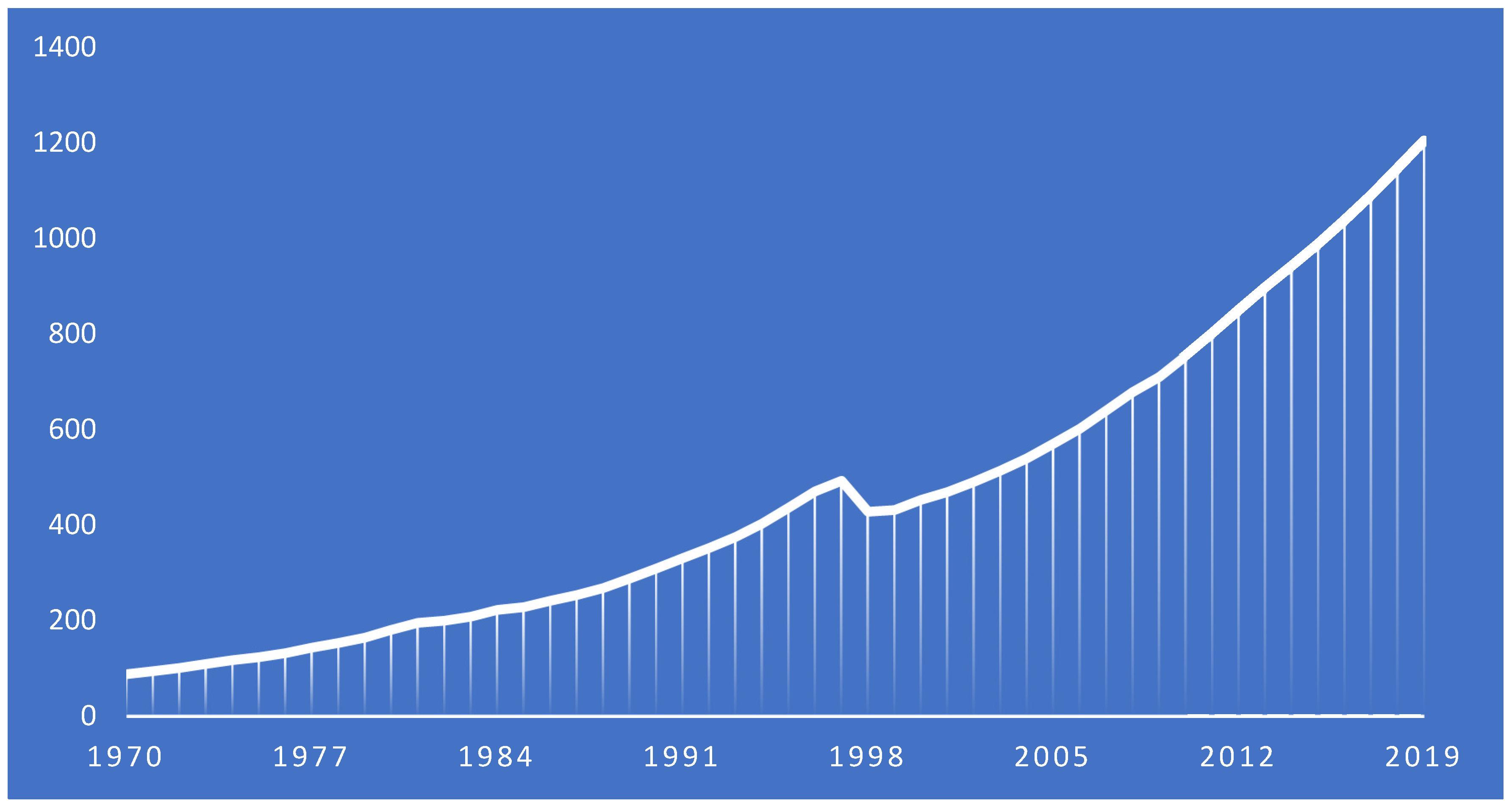
From 1970 to 2019, Indonesia’s GDP experienced a consistent upward trend as seen in
Figure 1. The country had an average growth of 5.52 percent per year, with the lowest (negative) growth of −13.1 percent in 1998 and the highest in 1980 at 9.88 percent. In almost 50 years, Indonesia’s GDP has increased by 1.258 percent or more than 12 times, from 88 billion rupiahs in 1970 to 1.2 trillion in 2019.
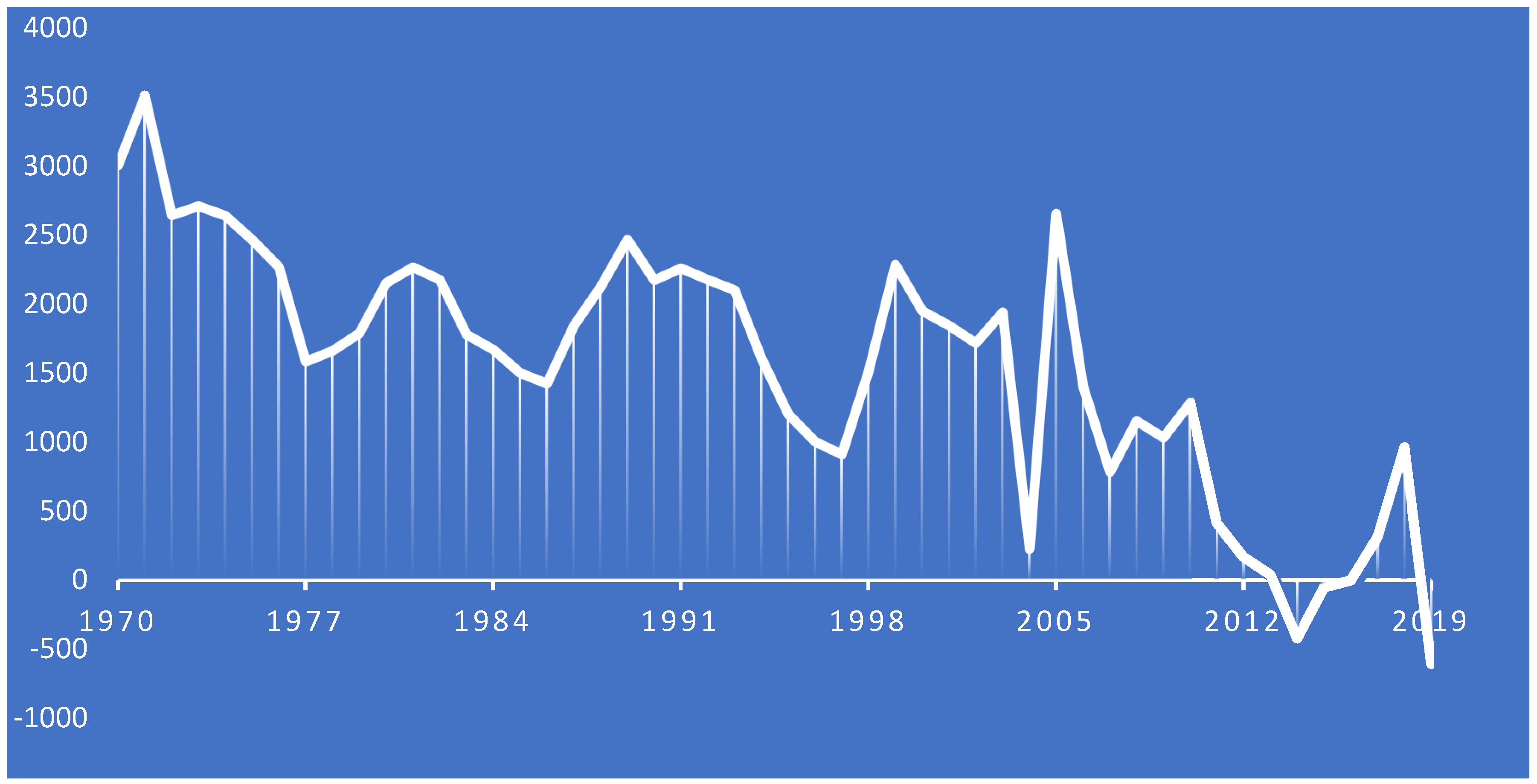
Generally, the Net Official Development Assistance (ODA) shows a downward trend from 1970 to 2019. However, as in the graph above, the development of ODA value is very volatile, with an average change per year of −73 million US dollars. The most significant decline of USD 1.4 billion (1.94 billion USD in 2003 to USD 228 million) occurred in 2004. Meanwhile, the steepest increase of US
$2.4 billion occurred in 2005. The highest ODA value happened in 1971 at US
$3.5 billion and the lowest in 2019 at US
$-605 million. During this period, the average ODA was 1.52 billion US dollars (
Figure 2).
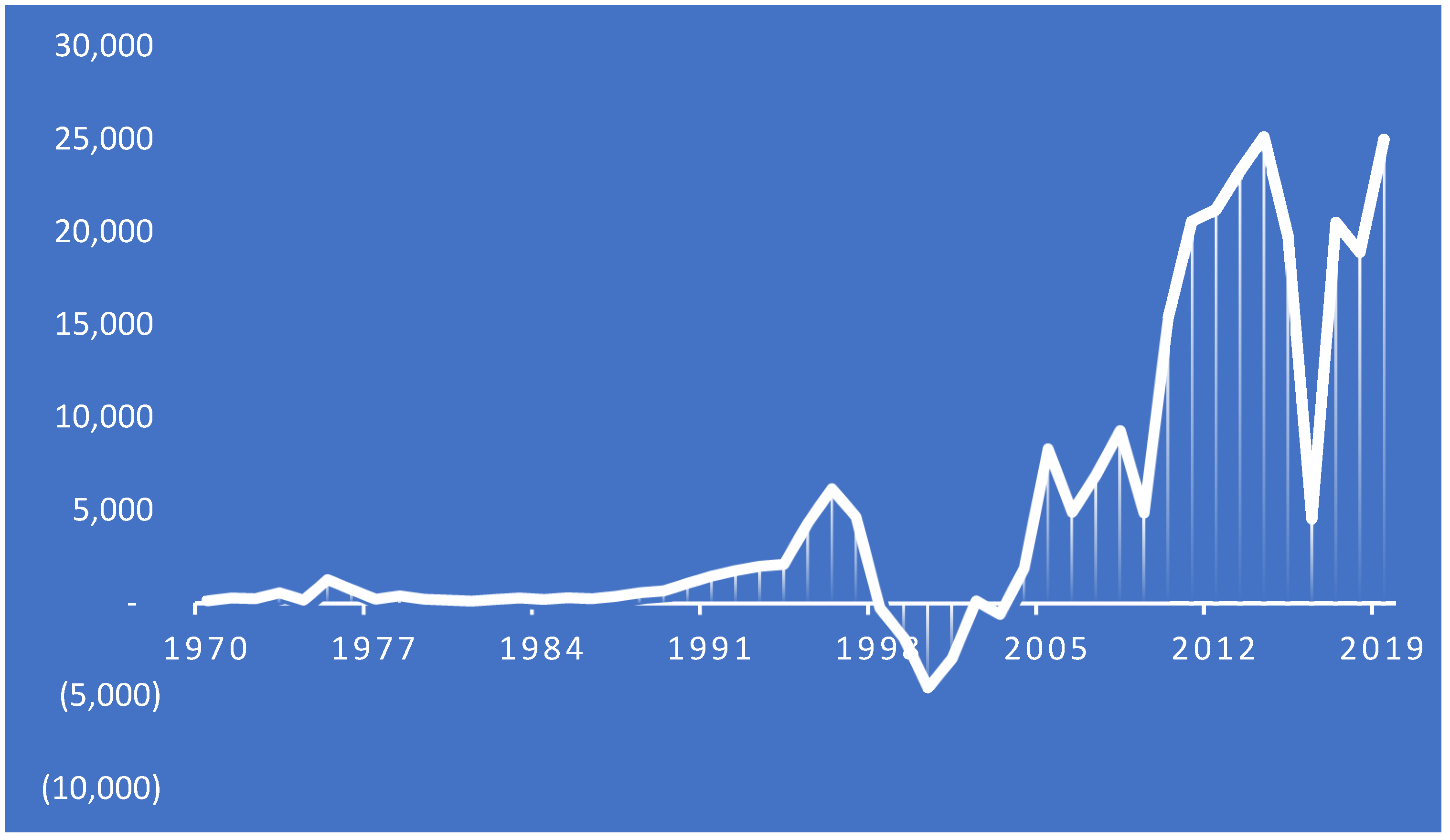
According to
Figure 3, Indonesia’s FDI net inflows appear to have a relatively low change in the period before 1990. This was followed by an increasing trend and a decline from 1997 to 2000, known as the period of the monetary crisis in Indonesia (and Southeast Asia). In this period, the lowest FDI net inflow of −4.5 billion US dollars was recorded from 1970 to 2019. The increase in FDI was also experienced in the early 2000s, with a sharp rise from 2010 to 2014. Furthermore, the highest net inflow value of 25 billion US dollars from 1970 to 2019 was recorded in 2014. After that peak, FDI net inflows fell over the next two years by more than 80 percent from 2014 to 2016 (25 billion to 4 billion US dollars). A sharp increase (350 percent) occurred in 2017 after the fall. In 2019 the value of FDI net inflow was USD 24.9 billion, which increased 171 times from 1970, which was only USD 145 million.
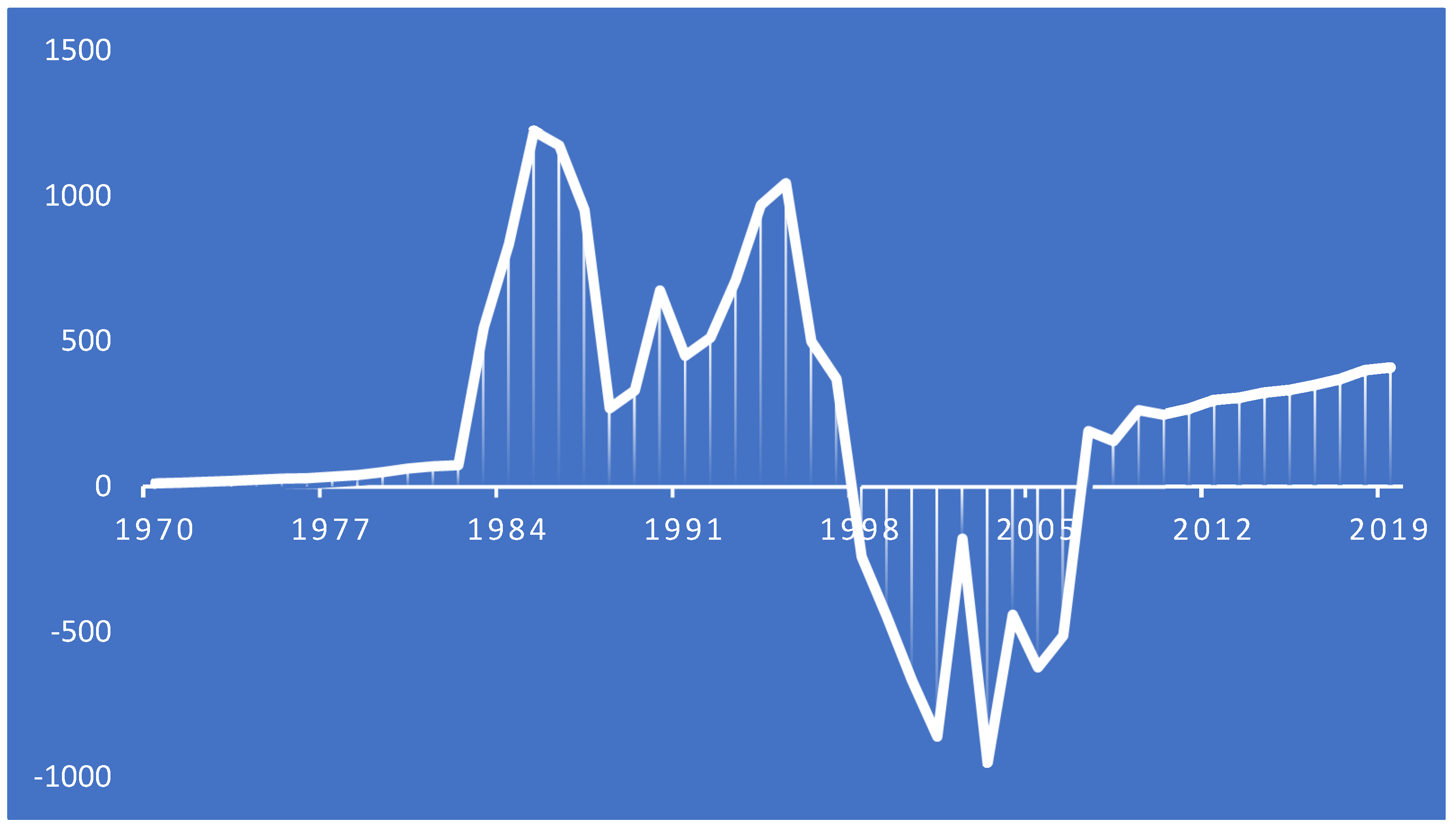
Figure 4 exhibits that Indonesia’s GCA experienced relatively stable changes from 1970 to 1982 and 2007 to 2019, with high fluctuations between these two periods. There was a sharp increase from 1982 to 1985 by 15 times, from US
$75 billion to US
$1.2 trillion, which was also the highest rise in GCA value in the period 1970–2019. GCA then fluctuated until there was a drastic decline after 1995 with a negative value in 1998 and reached its lowest value of −949 billion US dollars in 2003.
From 1970 to 2019, GDP, ODA, FDI, and GCA showed different trends. GDP was consistently positive, while ODA declined significantly during this period. FDI had shown a positive trend since the late 1990s and early 2000s with large fluctuations. Subsequently, as seen in
Figure 4, the GCA trend showed high fluctuations between 1982 and 2007 with low and positive changes outside this timeframe.
1.1. Economic Growth, ODA, FDI and Capital Formation
Capital formation is defined as generating capital assets and not using all of its resources for domestic development. Meanwhile, foreign aid (ODA) is a global strategy for alleviating poverty and improving the economy (
Adebayo and Kalmaz 2020;
Zhao and Du 2009). ODA is a form of Official Development Assistance and provides financial aid to promote developing countries’ economic development and welfare (
Minoiu and Reddy 2010;
Lee et al. 2020). Several studies have examined the relationship between ODA, FDI, and GCA with economic growth using different perspectives. However, the relationship between these variables is mainly mixed in both developed and developing countries.
Anetor et al. (
2020) examined 29 Sub-Saharan African (SSA) countries to determine the effect of FDI, international trade, and international aid on poverty reduction. The study used annual data for variables HDI, FDI, foreign aid, trade openness, GDP growth per capita, gross domestic formation, annual population growth, and inflation from 1990 to 2017 with the Feasible Generalized Least Square (FGLS) approach. The results of their study showed that the FDI level needed to eradicate poverty had not been achieved, and Foreign Aid had not been appropriately channeled. However, the study results showed that trade has a positive and significant effect on poverty alleviation, especially in SSA.
Numerous studies have been carried out to determine the relationship between growth and foreign aid, especially in developed and developing countries (
Farah et al. 2018).
Younsi et al. (
2019) examined the relationship between foreign aid and reductions in income inequality in 16 African countries. The study used an unbalanced panel annual dataset from 1990 to 2011 with a random effect model using robust OLS regression and system-GMM estimator. The results showed that foreign aid, foreign investment, trade openness, and corruption had a positive and statistically significant effect on reducing income inequality. Furthermore, government spending and inflation had a negative and statistically significant effect on reducing income inequality. Conversely,
Dutta et al. (
2016) explored the impact of foreign aid on government regulation regarding the business climate in 64 MENA (the Middle East and North America) and sub-Saharan Africa countries. The dependent variables tested were various measures capturing the regulatory climate of a country’s business, such as ease of opening a business, building warehouses, owning property, paying taxes, enforcing contracts, and closing businesses. While the independent variable was the flow of foreign aid in net official development assistance (ODA) and official aid (% GDP). This study analyzed panel data from 2004 to 2009 using the GMM estimator system analysis technique and the instrumental variable approach. The authors concluded that aid worsens the business climate by increasing government restrictions. This was because foreign aid provides recipient governments and political elites with the right resources to strengthen their power and predatory policies harmful to the business climate.
Research carried out by
Yiew and Lau (
2018) in 95 developing countries found a U-shaped relationship between foreign aid and economic growth. Initially, foreign aid had a negative impact on the country’s growth, and at a certain time, it positively contributed to its economy. Simultaneously, the study examines the impact of foreign aid (ODA) and FDI on economic growth (GDP) using Pooled OLS (POLS), Random Effects (RE), Fixed Effects (FE), and Fixed Effect Robust (FERB) regression models. Still from developing countries,
Ali et al. (
2019) stated that foreign aid has a significant adverse effect on the corruption level. Furthermore, it was also found that foreign aid lowered the corruption perception index, thereby leading to more corruption in the country. This study was carried out to analyze foreign aid (FA) on corruption in Pakistan, India, Sri Lanka, and Bangladesh. The variables analyzed are the corruption level, foreign aid, GDP per capita, democracy, the rule of law (public perception of applicable law), and political stability from 2000 to 2014. The analysis was carried out using dynamic ordinary least squares (PDOLS) and fully modified ordinary least squares (FMOLS) panels to estimate the coefficients of cointegrating vectors and the Granger causality test panel (
Granger 2004;
Matesanz and Fugarolas 2009).
Mahembe and Odhiambo (
2019) also conducted a study in 82 developing countries to examine the causal relationship between foreign aid, poverty, and economic growth. Their study used annual dynamic panel data from 1981 to 2013 with a panel unit roots approach, cointegration, and a panel vector error-correction model (VECM) Granger causality test (
Granger 2004). The results of a study by
Mahembe and Odhiambo (
2019) provide evidence that there is a two-way causal relationship between economic growth and poverty in the short term. In addition, a unidirectional causal relationship was also found between economic growth and foreign aid. Their study also empirically found a unidirectional causality between poverty and aid abroad. In contrast to the results of the short-term analysis, in the long run, it was found that foreign aid tends to converge on its long-term equilibrium path in response to changes in economic growth and poverty. In addition, economic growth and poverty together lead to foreign aid.
A relatively recent study carried out by
Adebayo and Kalmaz (
2020) examined the relationship between economic growth, foreign aid, trade, gross fixed capital formation, and inflation rates in Nigeria. The time-series regression analysis for the 39 years (1980–2018) used the Bound cointegration test, ARDL, and the time-frequency domain wavelet coherence approach. Their study confirmed that there is a long-run relationship between the indicators considered. The study also revealed that economic growth is significantly affected by foreign aid, trade openness, gross fixed capital formation, and inflation rates in the long run. The results of the wavelet coherence technique provide evidence to support the long-run estimation of this study, and the wavelet coherence results are supported by the results of the Toda–Yamamoto causality test.
Jena and Sethi (
2020) empirically tested the effectiveness of foreign aid by improving the prospects for economic growth in the sub-Saharan Africa (SSA) region from 1993 to 2017 from 45 SSA countries. This study is based on Pedroni and Kao’s cointegration test, the Johansen–Fisher Panel cointegration test, FMOLS, and PDOLS. They found that long-run and short-run relationships exist between foreign aid, economic growth, investment, financial deepening, price stability, and trade openness of the SSA economy. Moreover, there is also a unidirectional causality running from foreign aid to economic growth. The implications of this finding emphasize that the government in the region needs to design appropriate policy measures aimed at removing barriers; hence aid flows can be used more wisely to lead to optimal utilization of available resources.
Mallik (
2008) examined the effectiveness of foreign aid for economic growth in the six poorest and most aid-dependent countries in the Central African Republic using the Vector Error Correction Model approach. The study found a long-run relationship between real GDP per capita, aid and investment as its percentage, and openness. Furthermore, the long-run effect of aid on growth is negative for most of the countries studied. It seems that a large amount of aid to these countries meets humanitarian needs rather than increasing the economy’s productive capacity.
1.2. Economic Growth, Foreign Aid, FDI and Capital Formation
Many developing and developed countries are trying to attract FDI (
Anetor et al. 2020).
Table 1 summarizes previous studies on the association between economic growth, foreign aid, FDI, and capital formation. Findings from previous studies reveal that FDI has a positive or negative impact on a country’s economic growth. Similarly, a study carried out in Nigeria by
Olorogun et al. (
2020) found that FDI affects GDP. Furthermore, they also concluded a significant relationship between GDP and Financial Development of the banking sector, which is also corroborated by indirect causality from gross capital formation to the financial sector. Their study analyzes gross capital formation (GCF) and financial development of the financial sector (% GDP) from 1970 to 2018 using Pesaran’s ARDL bounds test and Toda–Yamamoto Granger causality and generally reinforces economic growth as a result of inflows. FDI, in the long run, through the financial sector, confirms that finance is the most crucial sector in the Nigerian economy.
Zellner’s Seemingly Unrelated Regression (SUR) method was used to analyze the effect of capital formation and FDI in 25 transition countries from 1989 to 2000.
Krkoska (
2001) found that capital formation is positively related to FDI, a substitute for domestic credit, and complements foreign credit and privatized income. The study concludes that an improved investment climate capable of attracting higher FDI inflows is likely to lead to higher gross fixed capital formation and more significant economic growth.
Belloumi and Alshehry (
2018) investigated the causal relationship between domestic investment, foreign investment (FDI), and economic growth in Saudi Arabia using annual time-series data from 1970 to 2015. This study uses the Autoregressive distributed lag (ARDL) bounds testing technique, fully modified ordinary least squares (FMOLS), dynamic ordinary least squares (DOLS), and the canonical cointegrating regression (CCR). Their analysis showed that in the long run, there is a negative two-way causality between non-oil and gas GDP growth and FDI, a negative two-way causality between non-oil and gas GDP growth and domestic capital investment, and a two-way causality between FDI and domestic capital investment.
FDI supports the economic growth of a country in both the short and long run. The study carried out by
Mowlaei (
2018) analyzed the effect of various forms of FCI, namely, foreign direct investment (FDI), personal remittances (PR), and Official Development Assistance (ODA), on economic growth in 26 African countries. This study used time-series data from 1992 to 2016 with Pooled Mean Group (PMG) econometric techniques. Mowlaei found that the three forms of FCI (FDI, PR, and ODA) positively and significantly affect economic growth in the long and short run, with the PR exhibiting the most significant rate. Previous studies have shown that GCA promotes economic growth. Therefore, the fiscal authority in a country is strengthened by expansionary fiscal policies stimulating economic growth, investment, and employment (
Pasara and Garidzirai 2020).
Pasara and Garidzirai (
2020) examined the relationship between economic growth, unemployment, and GCF from 1980 to 2018 using the Vector Autoregressive (VAR) approach in South Africa. The study empirically supports a positive long-run relationship between GCF gross capital formation and GDP economic growth. Moreover, they also found that unemployment does not affect economic growth (GDP) in the short run, with a significant and positive relationship between unemployment and GCF.
Gani and Clemes (
2003) examined the role of foreign aid on welfare in 65 developing countries (low-income and lower-middle-income economies) using annual data (1991–1995). For analysis, the authors used a pooled cross-sectional heteroskedastic and timewise (first-order) autoregressive procedure. The study showed that aid in education and water positively correlate with people’s welfare in low-income countries, while aid for education and health is positively correlated with their welfare in lower-middle-income countries. Moreover, output growth and gross domestic investment are positively associated with people’s welfare in low- and lower-middle-income countries.
In low-income countries, it is also found that unproductive government spending, conflict, and rural population are negatively correlated with people’s welfare.
Rani and Kumar (
2019) examined the long-run association and direction of causality between economic growth, trade openness, and gross capital formation for Brazil, Russia, India, China, and South Africa. This study analyzed time series data using the Applied Autoregressive Distributed Lag (ARDL) and vector error correction model. It showed that the unidirectional causality from trade openness to economic growth in India and Brazil supports the trade-led growth hypothesis. Meanwhile, bidirectional causality is found between trade openness and economic growth in China, supporting the feedback hypothesis. In South Africa, this study provides empirical evidence of a unidirectional causality moving from economic growth to trade openness, which validates the growth-driven trade hypothesis. Since trade openness is a significant determinant of economic growth in the BRICS (Brazil, Russia, India, China, and South Africa), member countries need to adopt policies toward trade liberalization to sustain economic growth.
In Iran,
Turković (
2017) investigated the relationship between capital formation and economic growth from 1974 to 2014. The variables analyzed are GDP per capita, exports (goods and services), FDI, gross fixed capital formation, value-added production, value-added services, government consumption, and labor force using the ARDL model and AFD (Augmented Dickey–Fuller) approach. These approaches showed that an increase in exports of goods and services and net FDI significantly affect economic growth. Furthermore, domestic sources of capital were found to promote economic growth and gross fixed capital formation.
Moe (
2008) studied Official Development Assistance (ODA) on human development and education in Southeast Asia countries, namely Cambodia, Indonesia, Malaysia, Myanmar, Thailand, Philippines, Laos, and Vietnam. The analysis was carried out from 1990 to 2004 using annual time series data and the OLS regression method. This study indicated that real GDP and FDI have a significant relationship with human development and education during the analyzed period. At the aggregate level, ODA has a significant positive relationship only with human development. This analysis also showed that ODA targeted to support socio-economic development has a significant relationship with human development.
Meyer and Sanusi (
2019) examined the causality between domestic capital formation and investment, employment, and economic growth in South Africa using quarterly data from 1995Q1 to 2016Q4. They found empirical evidence of a long-run relationship between domestic investment, employment, and economic growth. Besides, this study provides evidence that investment has a positive long-run impact on employment. The Johansen cointegration analysis and the Vector Error Correction Models (VECM) also showed bidirectional causality between employment and economic growth, while evidence of unidirectional causality from investment to employment is also found. Although there is a two-way causality between these two variables, economic growth does not mean an increase in employment in the long run, which confirms the existence of “jobless growth.” The investment proved to be a positive driver of employment in the South African economy in the long run.
By considering the synthesis of the previous studies above, the following hypotheses are formulated and tested in this study:
Hypothesis 1 (H1). Economic growth causes ODA.
Hypothesis 2 (H2). ODA causes economic growth.
Hypothesis 3 (H3). Economic growth causes FDI.
Hypothesis 4 (H4). FDI causes economic growth.
Hypothesis 5 (H5). Economic growth causes GCA.
Hypothesis 6 (H6). GCA causes economic growth.
4. Discussion
This study examines the causal relationship between ODA, FDI, GCA, and Indonesia’s economic growth from 1970 to 2019. The objectives are achieved in two steps. First, by carrying out a unit root test and cointegration to ensure that economic growth, ODA, FDI, and GCA integrated from the first order are related in the long run. This relationship is significant due to integrating two variables in the first order (I(1)). However, these variables are not related to each other unless they are cointegrated. The stationarity of the time series data used was checked using the ADF and KPPS tests. Based on the ADF test results, it is concluded that GDP and GCA are stationary at the first difference, while ODA is stationary at the level.
Furthermore, there is a unit root in the FDI variable at the level and first difference through the KPPS test. The ADF was continued with the degree of integration on the second difference, indicating that all variables were stationary. Therefore, time-series data analysis was continued with the formation of the VAR model. A cointegration test was performed using the Johansen to ensure the use of VAR or VECM. The results obtained indicate a stable long-run equilibrium relationship between the observed variables. The second step is to apply the causality TY framework developed by
Toda and Yamamoto (
1995) to determine the direction of causality between economic growth, ODA, FDI, and GCA.
The Granger Causality results based on TY estimation with the MWALD test showed that the null hypothesis, which stated economic growth does not cause ODA, and its meaning could not be rejected. On the other hand, it is found that ODA has causality to GDP, which also indicates that foreign aid plays a role in driving economic growth. Possible arguments include the effective allocation and use of foreign aid, where the return rate is higher than the investment level in Indonesia (
Adebayo and Kalmaz 2020). The explanation for the role of ODA in promoting GDP in this study is because the data analyzed is long-run time series with ODA in the proper form of assistance for a country’s economic growth. This is because it is transformed into development assistance supporting investments in physical infrastructure, organizational development, and human capabilities that produce long-run results (
Minoiu and Reddy 2010). Furthermore, ODA positively impacts the economy in countries with fiscal and monetary policies (
Burnside and Dollar 2000).
The null hypothesis stated that economic growth does not cause FDI and cannot be rejected. On the contrary, the hypothesis that stated that FDI does not cause economic growth can be rejected. Therefore, it is concluded that FDI has a positive role in economic growth and promotes GDP expansion with a positive causality rate in Indonesia. Studies carried out by
Olorogun et al. (
2020), and
Bird and Choi (
2020) stated that many factors make FDI directly impact GDP creation. These factors include promoting policies to support increased investment, creating a favorable economic environment to accelerate growth (
Meyer and Sanusi 2019). This is in contrast to the research undertaken by
Pasara and Garidzirai (
2020),
Rani and Kumar (
2019),
Turković (
2017), and
Meyer and Sanusi (
2019), which found the effect of domestic capital formation on GDP. The causality test results showed that is no causality in one or both directions between GDP and GCA. The underlying explanation is as follows. Capital formation does not guarantee economic growth in a country. Supposing capital accumulation is not followed by efficient resource allocation from less productive sectors to more productive with possible occurrence in the Indonesian context (
Blomstrom et al. 1994).
5. Conclusions, Recommendations and Limitations
The Official Development Assistance (ODA), FDI, and capital accumulation are elements used to ensure economic growth, including in Indonesia. Therefore, it is very interesting to examine the nexus between foreign aid, FDI, and capital accumulation on economic growth. Limited studies with long-time series data have been carried out to examine the relationship between these variables. Furthermore, the causality between foreign aid, FDI, and capital accumulation with economic growth using a causality approach and Toda–Yamamoto was not found. Therefore, this study uses a time series data span of 50 years (1970–2019), which was analyzed using Toda–Yamamoto Causality analysis to provide an adequate empirical contribution. The results reveal a one-way causality between ODA and GDP, as well as between FDI and GDP. This evidence also means that ODA and FDI are significant predictors of economic growth in Indonesia. Furthermore, the unidirectional causality relationship between ODA and GDP shows that foreign aid in the form of ODA leads to economic growth. Meanwhile, there was no causal relationship, either one-way or two-way, between economic growth and ODA, as well as FDI and the formation of capital accumulation are not statistically significant.
The findings in this paper also show that Indonesia’s economic growth is influenced by foreign aid and foreign direct investment. The policy implication of this finding is that foreign aid management needs to be optimized due to its ability to promote economic growth. Furthermore, special attention needs to be paid to attracting foreign direct investment, which has also been found to promote economic growth. One of the efforts is to create a macroeconomic and microeconomic environment capable of attracting FDI and government bureaucracies that can allocate ODA efficiently and appropriately to sectors that promote economic growth. To allocate ODA effectively, the government improves economic and institutional policies and encourages corruption eradication (
Jena and Sethi 2020;
Adebayo and Kalmaz 2020). Furthermore, to optimize foreign aid, monetary policy fiscal policy needs to be more credible from the perspective of foreign countries. Therefore, there is a possibility that foreign aid will not succeed in achieving the goal of promoting economic growth, supposing the Indonesian government is unable to create economic instability and combat corruption, as often found in developing countries (
Adebayo and Kalmaz 2020).
The study has limitations because it only focuses empirically on examining the causality of ODA, FDI, and GCA with Indonesia’s economic growth. These are economic variables, and when the analysis is added by including demographic variables, bureaucratic management, and environmental aspects, it is likely to produce more comprehensive findings by analyzing factors and variables associated with a country’s economic growth. Furthermore, since FDI was found to promote GDP, the Indonesian government needs to encourage improvements in the political and economic framework because the sustainability of FDI depends on the environmental quality of the recipient country (
Olorogun et al. 2020). Therefore, FDI needs to be supported by policies to allocate more productive projects that promote economic growth for FDI to remain a stimulator of GDP creation (
Belloumi and Alshehry 2018;
Krkoska 2001). In addition, this study also does not include monetary economic variables in the regression model. Future research needs to include such variables as predictors of economic growth.


