1. Introduction
Since the deployment of the first satellite with a synthetic aperture remote sensing system into orbit in 1978 [
1], the use of SAR imagery has been a vital part of several scientific domains, including environmental monitoring, early warning systems, and public safety [
2].
The SAR functioning principle can be described as follows [
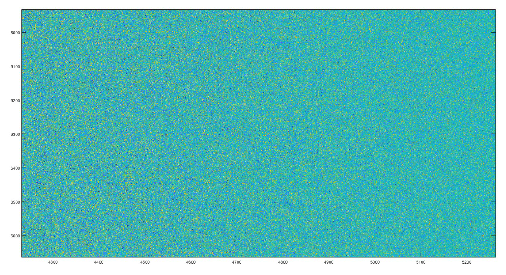
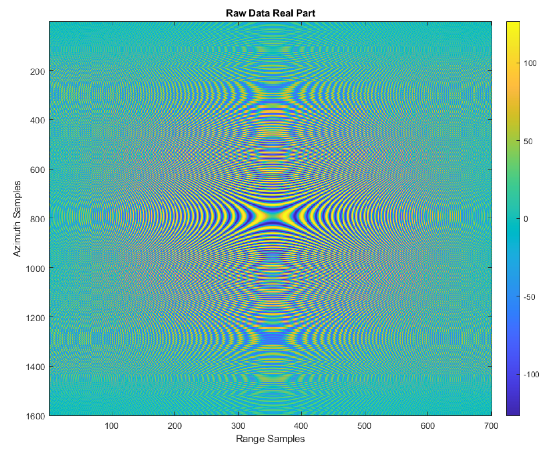
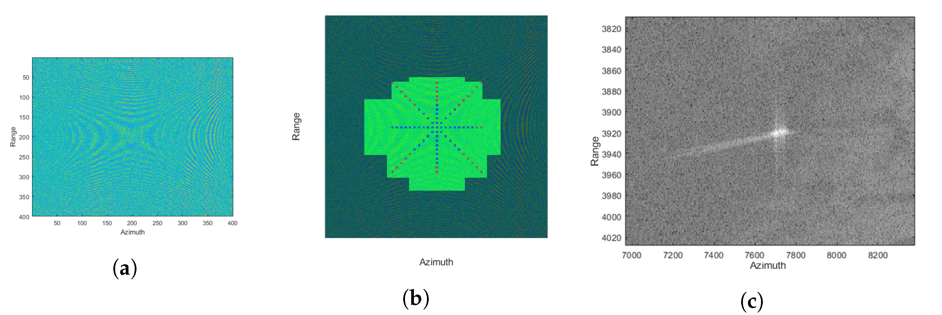
3]: microwave signals are emitted from a radar mounted on a moving object, such as a satellite, and later, the back-scattered signals (echoes) are collected to generate raw data. The motion of the sensor is opportunistically used to synthesize a very long antenna and obtain a high-resolution image of the scene being observed by properly integrating the collected raw data. SAR is distinguished from other mapping techniques by its active operational mode. In fact, the sensor has its own energy source for illuminating the local region. Thanks to this, SAR permits service regardless of solar radiation or time of day. In addition, it is possible to select the transmitted wavelength in a specific range wherein the attenuation of electromagnetic waves generated by the atmosphere can be neglected. As a result, the SAR sensor can work in the day, night, and nearly all weather conditions and can even monitor a cloud-covered region. SAR could be described as “non-literal imaging” since the raw data do not resemble an optical image and are incomprehensible to humans (see
Figure 1). For this reason, SAR raw data are typically processed by means of a focusing algorithm that, in a nutshell, implements space-variant two-dimensional filtering of raw data. More specifically, the focusing step uses the motion of the sensor to synthesize a very long antenna and obtain a higher-resolution image of the scene being observed. The result of this process is a complex image, known as a Single Look Complex (SLC) image. The generic pixel of the SLC image corresponds to a specific cell on the ground. The phase of the image is typically used to extract information about the sensor pixel distance in interferometric applications related to Digital Elevation Model (DEM) generation [
4] and ground motion monitoring [
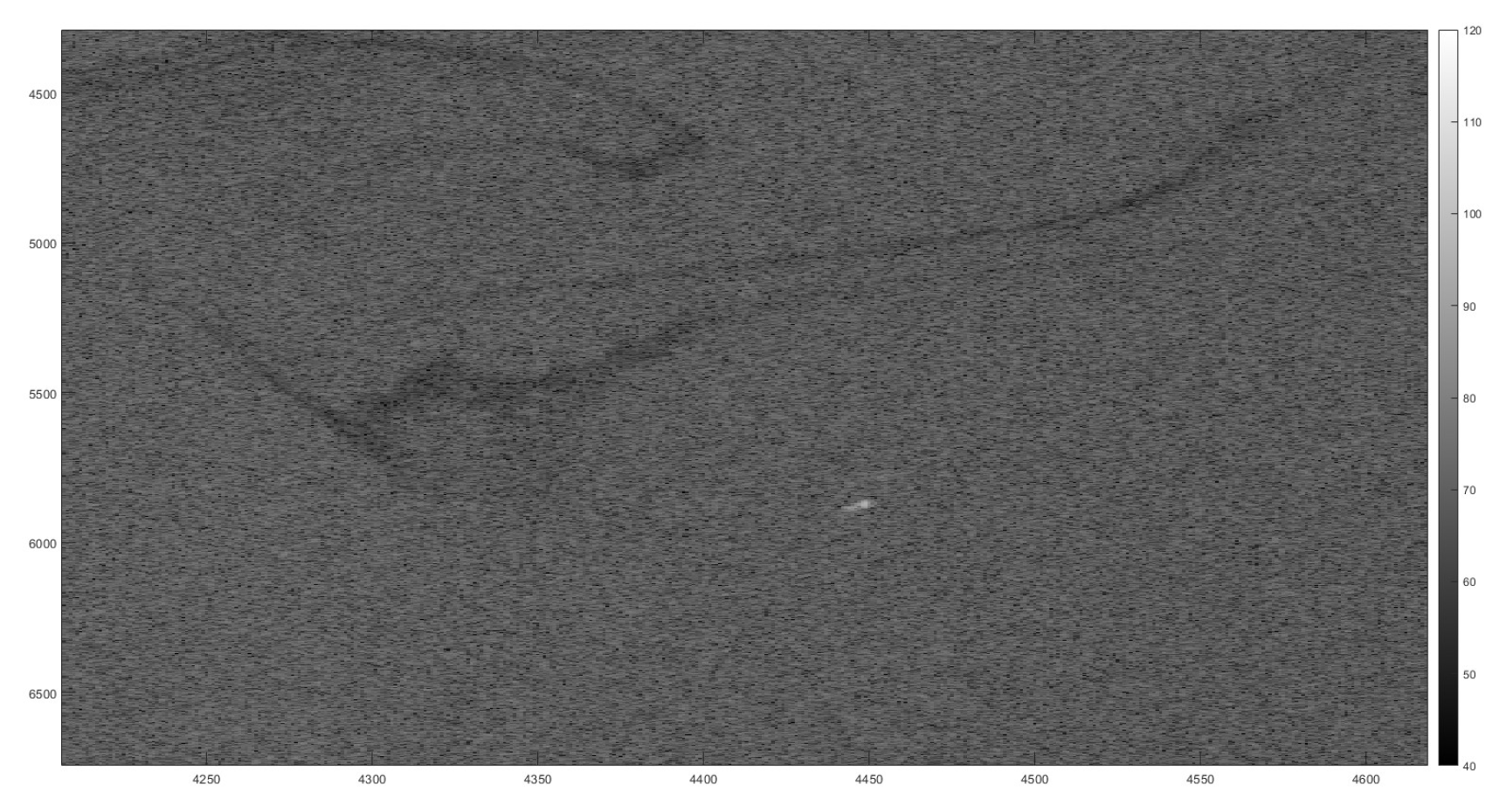
5]. The amplitude of the image is related to the backscattering coefficient of the cells on the ground and is typically used in segmentation and classification applications, such as oil and ship detection (see
Figure 2).
Although several efficient focusing approaches are available in the scientific literature [
6,
7,
8,
9], the processing of raw data requires a significant amount of computational power. Moreover, focusing represents only the first step of the detection process since it may be necessary to introduce further processes, such as calibration [
10] and despeckle filtering [
11], before proceeding with the actual detection phase. As a result, it is almost never practical to perform it onboard, and consequently, the data are transmitted back to Earth to be processed. This introduces a non-negligible latency, which is the main limitation to the implementation of SAR-based real-time services. This is the case, for example, for oil and ship detection services. Although the potential of SAR data has been well demonstrated and consolidated for maritime surveillance [
12,
13,
14], the latency due to the transmission of radar data to the ground segment currently represents a strong limitation.
In this scenario, onboard detection would represent an interesting solution to the problem thanks to the possibility of performing detection as soon as data are taken, thus also enabling transmission to the ground segment of alert signals only, with a notable reduction in both latency and downlink bandwidth. However, as already mentioned, the reduced computational capabilities onboard prevent the application of algorithms adopted on ground computing centers and even the simple focusing step can represent a complex operation from a computational point of view. The objective of next-generation studies [
15] is then to optimize Earth Observation (EO) data processing in order to deliver EO products to the end user with very low latency using a combination of advancements in onboard processing. As a result, in the field of the EO, the demand for real-time decision-making capabilities jointly with the need to optimize data acquisition and transmission has led to a significant interest in onboard intelligence, particularly in scenarios such as the early detection of disasters, extreme events, maritime situation awareness, and automatic target recognition, where swift and informed decisions can mitigate potential risks and minimize impacts and damages [
16].
In this scenario, Artificial Intelligence (AI) can provide the needed boost, thus allowing new applications to be realized [
17], by focusing directly on the information contained in the data, autonomously extracting relevant features for a given application. In particular, as highlighted in [
18], Convolutional Neural Networks (CNNs) have demonstrated remarkable results in several space applications, such as scene classification, object recognition, pose estimation, change detection, and others; while the initial paradigm was to have these applications run using a server-hosted processor, recent advances in microelectronics provide efficient hardware accelerators enabling the implementation of AI algorithms “at the edge” [
19]. Furthermore, according to [
18], mission lifetime extensions, as well as improvement by means of delta training, could also be immediately feasible for AI solutions via dynamic reconfigurability of the CNN.
However, as pointed out in [
16], the research on Edge Computing (EC) to reduce the amount of data transmission and energy consumption in EO applications is still in its infancy. As a response to this demand, preliminary research activities have been directed toward the exploration of onboard intelligence for EO applications based on optical sensors. In particular, the ability to run Machine Learning (ML) algorithms with EO-oriented platforms has been demonstrated by SmallSat missions with optical payloads such as
sat missions, using off-the-shelf ultra-low-power AI-optimized chips [
18]. As of today, it is noteworthy that fewer efforts have been dedicated to SAR sensors in comparison to optical sensors. This is also well recognized by the European Space Agency (ESA), which has recently launched several initiatives (e.g., the onboard intelligence for SAR missions invitation to tender) in which it is recognized that, despite the immense potential of SAR, it remains an under-explored domain in terms of onboard intelligence implementation. One of the main reasons identified by ESA is the complexities arising from onboard SAR data’s inherent characteristics with unfocused SAR raw data, including its complex interactions with the Earth’s surface, that present challenges (but also opportunities) for integrating intelligent decision-making processes directly into SAR-equipped spacecraft. For these reasons, approaches based on detection applied directly to raw data may represent a possible solution that requires more investigation. More specifically, the accuracy and computational cost of these approaches are both of extreme interest as they are not sufficiently addressed in the literature. In this regard, the present work analyzes the ship detection accuracy that can be achieved by using a Convolutional Neural Network directly applied to SAR raw data.
Recent studies have indicated that CNN might outperform human performance in a variety of fields [
20,
21]. As described in a dedicated recent survey [
22], CNNs have also received increasing attention from researchers in target detection with SAR images and have evolved rapidly, achieving interesting results in many application fields. More specifically, in [
22] traditional detection algorithms are classified into three categories (based on structural features, gray features, and texture features) and are compared with CNN-based algorithms, highlighting the interesting advantages of deep learning, mainly consisting in the capability to (i) achieve high classification accuracy, (ii) accurately extract high-level features, and (iii) provide strong robustness and adaptability to complex environments. However, all the traditional and CNN-based approaches analyzed in [
22] and the references therein introduce a preliminary pre-processing stage that involves, at least, the focusing step and possibly despeckle filtering. The (traditional or CNN-based) detection stage is then applied after the pre-processing stage. It is also interesting to note that both focusing and despeckling are effectively spatial filtering operations (space-variant or space-invariant, depending on the chosen algorithm) and, therefore, can ultimately be mathematically described using the convolution operation. Considering that CNN is a typical deep learning model that uses convolution operations and non-linear mapping to effectively extract target features, there exists a need to further investigate approaches that could integrate pre-processing and the detection stage into a single CNN algorithm, thus working directly on raw data. More specifically, our study attempts to eliminate any pre-processing by training a CNN to directly recognize ships on raw data. We only focused on the feasibility of detection, while computational cost is not within the scope of this work, even though the possibility to skip some pre-processing steps intrinsically opens new scenarios to substantially shorten processing and delivery times.
In this analysis, it must also be considered that, in recent years, the visual attention mechanism used by humans to deal with complex visual signals (selecting relevant information and filtering out irrelevant information) has gained attention in the fields of object detection and image quality assessment [
23,
24]. In [
25], a novel SAR image target detection method based on a visual attention model is proposed with performance that, in simulation tests, shows good capability and robustness compared to traditional algorithms such as Constant False Alarm Rate (CFAR). However, these encouraging results are obtained on focused SAR images where the target response is concentrated in a well-confined pixel area. On the contrary, in raw images, the radar target response is spread over several thousands of pixels, and very often, it is not detectable by the human eye (as illustrated later in this paper), thus leading us to avoid testing this approach in this work and leaving it for future research activities.
Another important aspect of this work concerns training data sets that, as well known, are critical to the development of machine learning algorithms [
26,
27]. In this regard, the efficacy of the final machine-learning-powered solution for a specific application is ultimately determined by the quality and amount of the training data. In particular, as detailed in [
28], a major challenge in using CNNs in the SAR domain is the availability of large (and realistic) data sets with annotated SAR data, thus introducing overfitting risk. This is particularly true for training data sets based on raw data. As a result of the above challenges, the scientific literature proposes transfer learning techniques focused on the transfer of knowledge from a secondary related domain, where labeled data are easy and inexpensive to obtain. For example, refs. [
29,
30] give details concerning transfer learning based on optical images. Alternatively, the use of SAR simulators can also be a valid approach, as detailed in [
31], where it is shown that a simulated SAR data set can be transferred successfully to a real SAR data scenario.
Four possible approaches are then available to produce, in the present work, a suitable training data set for raw-data-based ship detection: (i) the use of real data extracted from SAR images, (ii) the use of optical-based transfer learning, (iii) the use of an SAR data simulator, and (iv) the use of a hybrid approach (real and synthesized data combined together). All of these approaches have advantages and disadvantages. The approach based on the use of real data allows the training of the CNN in conditions similar to those of the operational service, but data generation is, in general, a time-consuming activity. The use of transfer learning and SAR simulators allows the quick production of a very large number of training data but may produce unrealistic data. The hybrid approach can represent a compromise between the two previous approaches, but it can also represent a complication related to the lack of harmonization between real and simulated data.
In our work, we mainly wanted to give priority to the ability to have physical control of data set generation at the expense of the complexity of the SAR scenes; therefore, we adopted a simplified simulation approach. This choice will provide a quantitative analysis of the applicability of a simple simulation tool in real application scenarios. The proposed simulator produces a set of complex matrices simulating SAR raw data acquired in a marine environment with the presence of ships. The synthetic data set was then used to train and evaluate a state-of-the-art CNN. More specifically, the simulator developed is based on the parameters of the ERS SAR mission, which is a well-documented system [
32] and, therefore, lends itself to the simulation of data sets in realistic conditions. As already stated, the simulation approach is based on a low level of complexity aimed at developing a fast and automatic simulator. The adequacy of this choice was subsequently verified by evaluating the CNN performance with real data extracted from ERS images. The scientific literature provides many applications of ERS data to the maritime context [
33,
34], and this allows the easy identification of case studies to be used for the test of the proposed CNN in real scenarios.
2. Materials and Methods
As described in the previous section, this study is aimed at the implementation of a CNN-based approach capable of detecting ships directly on SAR raw data. This required two main steps:
- -
The implementation of an SAR simulator of raw data in a maritime environment;
- -
The configuration and training of the selected CNN by using the training data sets generated with the SAR simulator.
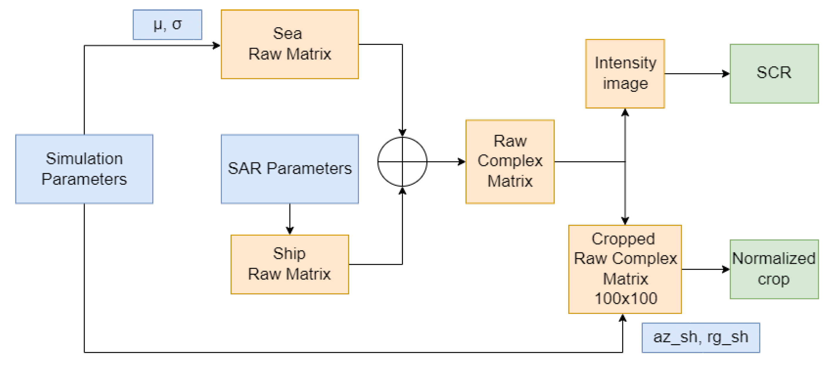
As already stated, the implementation of the simulator followed an approach based on a low level of complexity aimed at developing a fast and automatic simulator. More accurate approaches based on, for example, advanced physical models have been discarded due to the large number of external parameters to consider and their complex interaction. This would implicate a challenging activity with the implementation of a complex simulator that may lead to the generation of training data sets based on data extraction from real images, which is not the strategy that we wished to adopt in our work. As a result, we simplified the simulation of the sea and ship raw data set according to the block scheme presented in
Figure 3. Details for each block are addressed in the next subsections.
2.1. SAR Parameters
As already mentioned, the real and simulated data are based on the ERS-1 and ERS-2 satellites. Although these satellites no longer operate, they together represent, even still today, one of the most successful satellite SAR missions. The ERS-1 satellite was launched in 1991, followed by ERS-2 in 1995. The two ESA satellites, at the time, represented the most technologically advanced Earth-observing spacecraft that had ever been manufactured in Europe and were able to collect data for more than fifteen years, thus generating a very wide data set suitable for both land and sea applications with a very extensive bibliography [
35].
The main ERS parameters are listed in
Table 1. The values are derived from parameters defined in the ERS handbook [
32]. The ERS operating frequency falls in the C band that, according to IEEE designation, spans from 4.0 to 8.0 GHz, which is a typical operating band for Earth Observation radar systems. Additional parameters that depend on the specific acquisition time, such as the radar’s altitude and velocity, can be extracted from the auxiliary files associated with each image. For our simulator, we used the average values indicated in
Table 2.
2.2. Ship Simulation
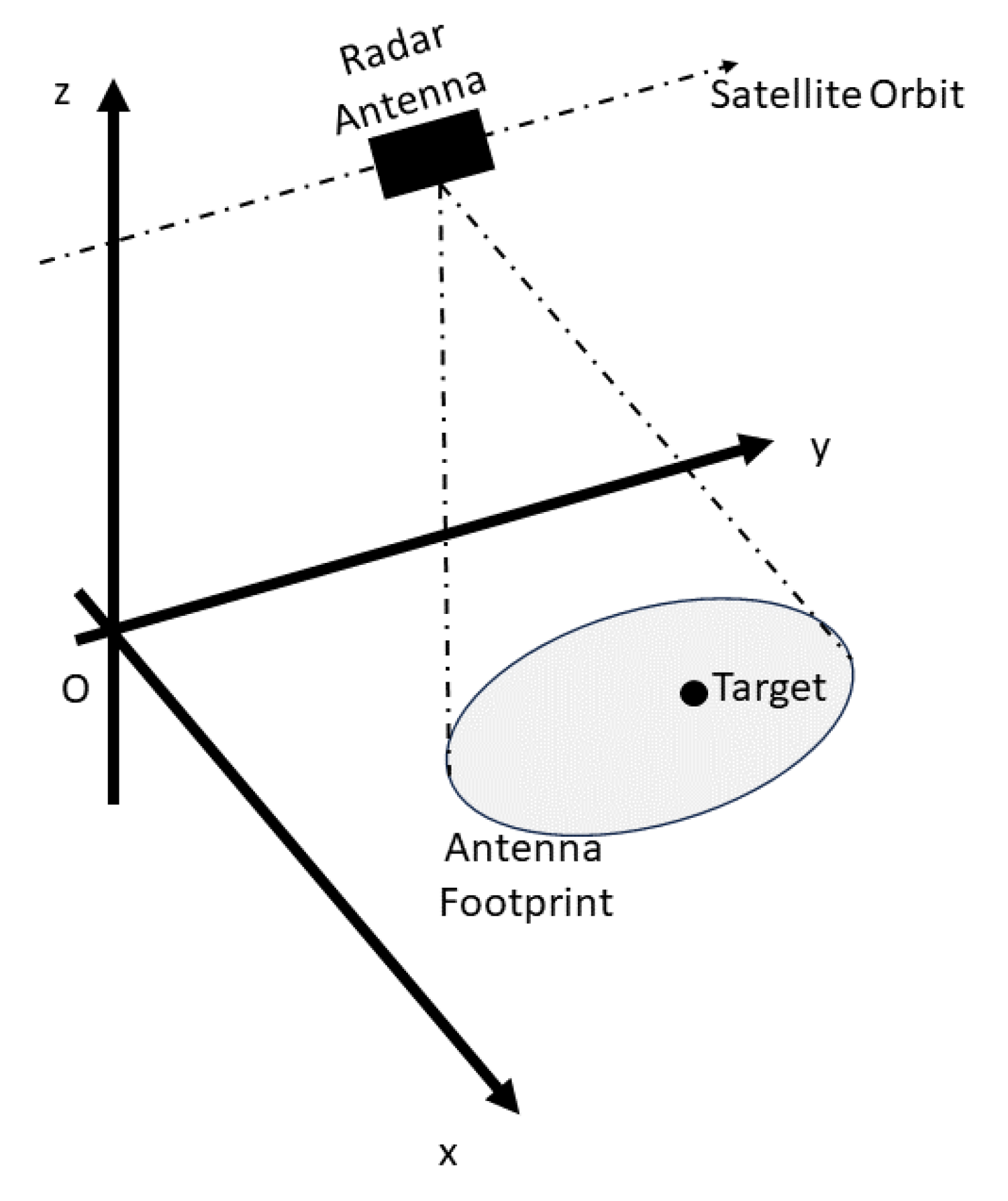
The SAR response of a ship depends on many factors, such as the material, shape, dimensions, and orientation of the ship toward the radar acquisition system. For this reason, we propose an approach aimed at implementing a minimal level of complexity in the simulation of a ship’s response, choosing the single-point model. The SAR signal model used for the implementation of the simulated data set is based on the acquisition geometry depicted in
Figure 4.
The SAR sensor travels along a flight path (known as the azimuth direction) such that the antenna phase center, at a given instant
, has a three-dimensional spatial location denoted by:
In this acquisition geometry, a generic stationary (or slowly moving) point target located in the scene has the following coordinates:
The distance from the antenna phase center to the target, known as range, is denoted by:
At periodic intervals (given by the inverse of the pulse repetition frequency), the radar antenna transmits a pulse, known as chirp and defined by the following equation:
where
is the amplitude of the transmitted signal,
is the duration of the chirp signal,
is the carrier frequency,
is the chirp rate, and t is the time axis centered in the generic instant
when the transmission occurs.
The point target on the ground receives this signal and produces a so-called echo, which is a delayed and rescaled version of the transmitted signal, as defined by the following equation:
where c is the speed of light,
is the magnitude of the received signal and is different from
since it takes into account the energy loss during propagation and reflection, and
represents the phase change that may result from the target scattering processing. The time delay of 2
(
)/c takes into account the two-way propagation from antenna to target.
The received signal is demodulated in order to remove the carrier frequency:
Finally, the received demodulated signal is sampled (at
= n/
) and quantized in order to obtain a discrete-domain signal. The sampling frequency used in the ERS mission produces
= 704 range samples for the chirp signal. It can be observed that the antenna footprint allows the collection of several echoes from the same target in different
instants. In particular, for the ERS case, we used a realistic value of
= 1600 echoes. As a result, a single-point generates an overall ERS impulse response that takes about 700 samples in the range direction and about 1600 samples in the azimuth direction:
where
m and
n are the matrix coordinates of the azimuth and range directions, respectively.
As illustrated in the simulation of
Figure 5, despite the single-point simplification, it must be noted that the relevant raw data generated are a complex matrix, wherein rows represent azimuth samples and columns represent range samples, with azimuth being the flight direction of the satellite and range being the look direction (distance) of the SAR sensor. Although this is a considerable simplification, it has proven to be extremely useful for verifying whether the training of the selected CNN in such conditions is still valid enough to subsequently operate with real data.
Once the single-point impulse response is available,
(m,n), it is possible to generate raw data images with a generic position of the ship by simply adding a range and an azimuth shift by means of the following equation:
where the parameters
and
are the applied shifts according to the block diagram of
Figure 3.
It is interesting to note that the typical SAR focusing step is in charge of collecting all the echoes and ideally compressing their energy in a single pixel located at coordinates
and
. This is obtained by means of several techniques proposed in the literature [
6,
7,
8,
9] that efficiently implement a 2D convolution with a matched filter
, thus obtaining a focused SLC image:
2.3. Sea Simulation
A realistic marine simulation is a difficult goal to attain. Many factors must be considered, including weather, wind, sea state, marine currents, biological spots, and oil slicks. For this work, we propose a simplified approach based on a statistical model of the sea directly derived from the distribution of the values of the raw data.
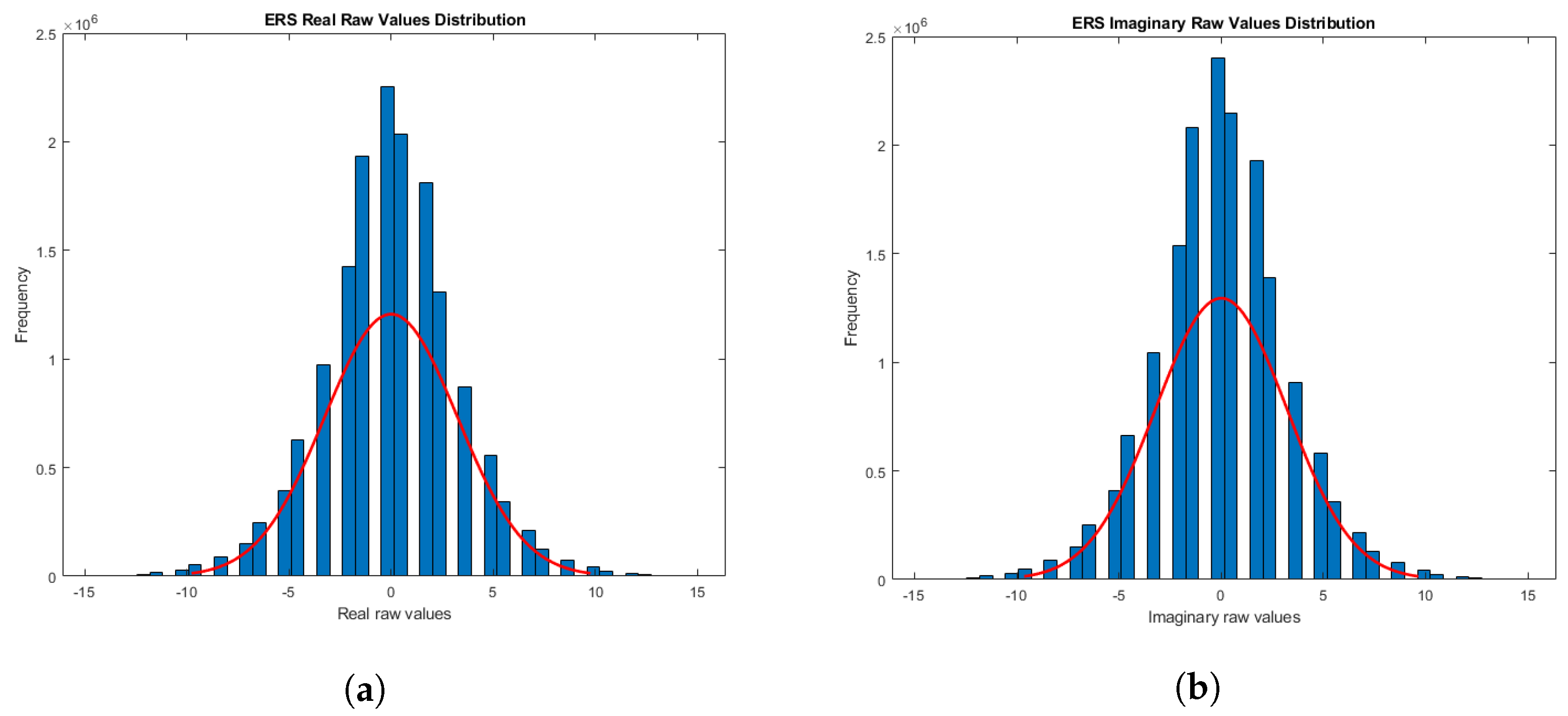
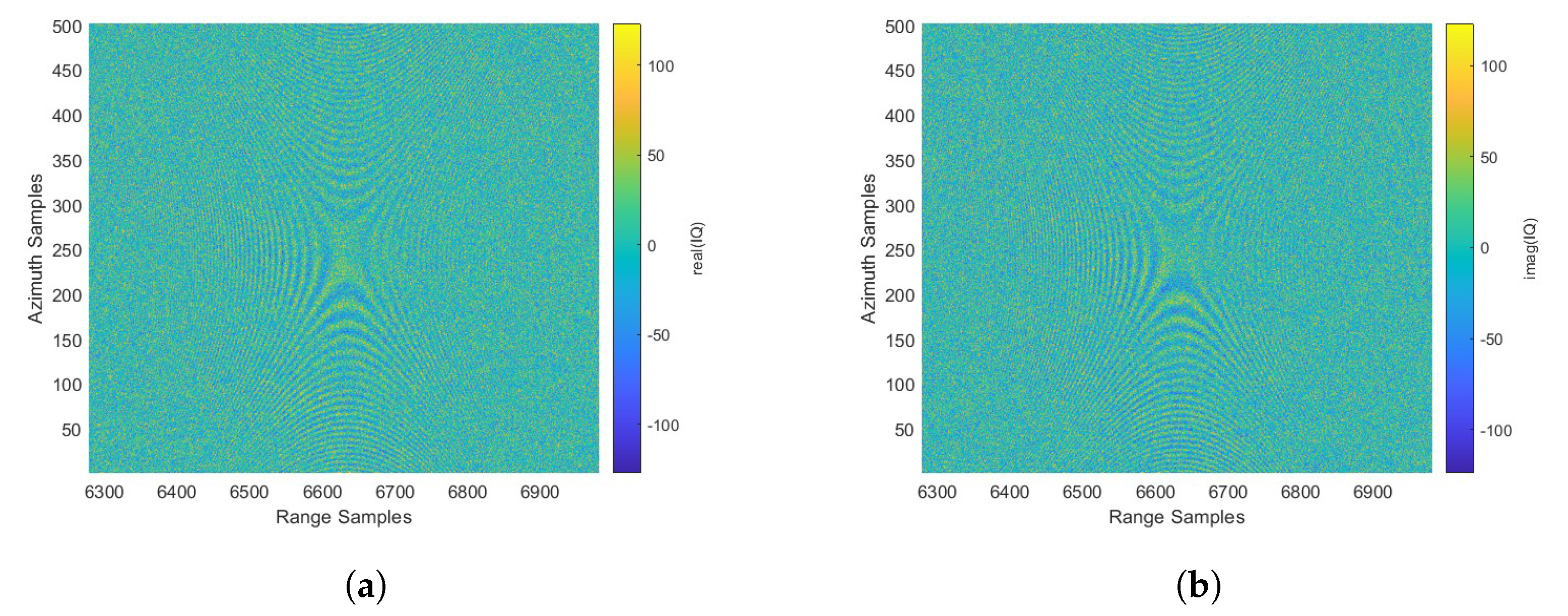
As outlined in [
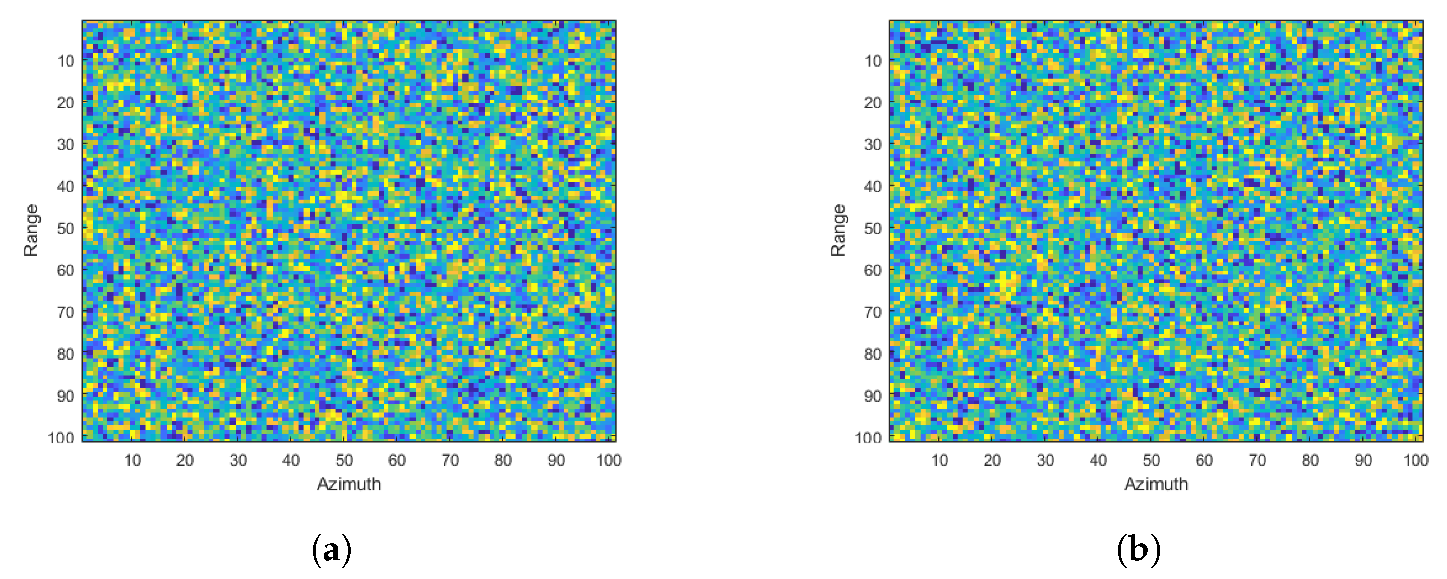
36], either in the high-resolution or low-resolution case, with the ideal hypothesis of a sea background having a constant radar cross section and the central limit theorem, both the real and imaginary parts are Gaussian-distributed. Although more complex modeling can be proposed, the analysis carried out on a number of different crops of ERS-1/2 raw complex data (see
Figure 6) shows that it is acceptable to model both the real and the imaginary parts with a truncated Gaussian distribution according to the following equation:
The four variables used to characterize the truncated Gaussian distribution are the mean (), the standard deviation (), and the truncation limits ( and ). In particular, for our simulation, the following were employed:
- -
was set to 0;
- -
was varied in order to generate different rough sea conditions, i.e., different levels of the sea signal with respect to the ship signal, thus obtaining different Signal-to-Clutter Ratio (SCR) values;
- -
The truncation limits were set according to the quantization of the real and imaginary parts performed by the 5-bit analog-to-digital converter of the ERS acquisition system. This allows the quantized data to take integer values in the range of −16 () to +15 ().
The simulation is simply implemented by initializing an empty matrix with complex values by using random values generated via the truncated Gaussian distribution (here indicated with
). This matrix represents the raw data generated from the sea return:
where
i is the imaginary operator and
(m,n) and
(m,n) are real matrices randomly generated with the truncated Gaussian distribution.
2.4. Training Data Set Generation
In accordance with the block scheme illustrated in
Figure 3, once a pair of sea and ship simulations are produced, these two contributions are summed into a single complex matrix that represents the simulated noisy raw data image:
In this way, we introduce full control of both the reference image (the ship radar response,
) and clutter (the sea radar response,
), with the possibility of conducting parameter sensitivity tests in terms of noise intensity and ship extension and position, as detailed later in this paper. This approach allowed us to perform an exhaustive sensitivity analysis, thus avoiding (at least in this study) working with blind quality assessment approaches that are very common in the literature [
37,
38,
39].
After this stage, the simulator activates two branches aimed at the generation of the training data set and computing image quality. It must be noted that high-quality training data are important for the successful use of intelligent systems. Various survey works are available in the literature regarding the estimation of the quality of an image, known as Image Quality Assessment (IQA) [
40,
41]. In the specific case of this work, it was decided to take as a reference the Signal-to-Clutter Ratio (SCR), which is a specific parameter used in the SAR field, largely employed in the field of ship detection [
42]. It is useful in our work to verify whether the raw data generated in the simulation are capable of producing an SAR response with the presence of an intensity peak in a noisy background.
To this aim, it was inserted in the block diagram of
Figure 3, a branch dedicated to focusing the simulated raw data and the subsequent calculation of the SCR. More specifically, the first step generates the intensity image, obtained by focusing the raw data and computing the magnitude of the result:
Subsequently, the SCR is computed according to Formula (
14).
where
is the peak intensity of the ship return, while N is the average intensity of the sea around the ship. These two parameters are computed on the intensity image
.
There is an alternative to this expression, where P is calculated as the average power of all the pixels belonging to the ship. This second version, however, is susceptible to estimation errors on real data since it is not possible to know precisely the extent of the ship in the image. This second expression is very common in the scientific literature; we will refer to it with the notation SCR in this paper.
In parallel, a second branch of the block diagram extracts a crop of the simulated raw data image that contributes to populating the training data set. For this study, we looked at the effects of different cropping dimensions on raw data. Following several tests, we determined that the best performance dimension was 100 × 100 samples, which is significantly shorter than the impulse response. A possible explanation is that, in this way, we can concentrate the crop on the peak response, which typically contains significant energy of ship radar return, and guide the selected CNN to learn to identify this part of the signal, which is less disturbed by the background noise generated by the sea response.
Furthermore, the selection of a small crop introduces two other advantages. First, it must be considered that the CNN we will examine in the next sections of the paper is a classification network; this means that it does not specify where the ship is in the scene, but whether it is present or not. The use of small crops is, therefore, recommendable in order to reduce uncertainty about the ship’s position. Second, a smaller crop requires less training and classification times. To make the simulation closer to realistic conditions, the ship position is not centered in the crop; it is moved from the center with a random shift of ±12.5 pixels in the range and azimuth directions (
az_sh and
rg_sh parameters are shown in
Figure 3). The goal of this shift is to improve ship detection performance even when the ship peak is not exactly centered in the crop.
2.5. Convolutional Neural Network
The goal of the Neural Network is to categorize the raw data crops into two classes: Ship and NoShip. Due to the fact that input raw data are a complex matrix, the selected CNN was configured to work with two separate real channels representing the real and imaginary parts of the input data, respectively (see
Figure 7). In a preliminary analysis, we also attempted to work with only a single real channel selected among the real part, imaginary part, amplitude, and phase of the input complex data, but none of them provided satisfying results. Therefore, the use of both real and imaginary channels was the final choice for the present work, and only the results concerning this choice will be presented.
Since the main objective of the present work is to prove the feasibility of ship detection on SAR raw data by means of a CNN approach and not to test different machine learning algorithms, it was necessary to choose an algorithm with a high probability of success in the proposed experiment. To this aim, we evaluated the performance of a deep neural residual network known as “ResNet” [
43] that can be considered a state-of-the-art Convolutional Neural Network. CNNs are a class of deep learning models designed to process and extract features from visual data, such as images and videos. These networks employ convolutional layers to detect local patterns and hierarchical structures, followed by pooling layers to reduce spatial dimensions and increase computational efficiency. The fully connected layers at the end of the CNN interpret the learned features to perform classification or regression tasks. Deep convolutional neural networks, during the learning phase, use kernels that are normally randomly initialized and, in the subsequent phases of convolutions and max pooling, the kernels able to extract the information necessary to justify the class of belonging of the input crop are retained, while the others are discarded.
The network working on a generic case of the absence of the ship (null hypothesis) works only on sea images. Such images are obtained as described in [
11]. No pattern is recurrent in the learning phase, so the network chooses the most similar patterns from the background noise for each crop in the training set corresponding to the null hypothesis; such kernels are not present on all training image sets, so the decision process is chosen on this basis for the null hypothesis. If a ship is present in the image, a specific pattern appears to be present in the input data and is recurrent on all the crops in the training set of the detected hypothesis; thus, max pooling extracts the kernels able to detect this kind of pattern. The convolutional neural network is useful in our application as many crops can contain patterns only in a small part of the image while the rest may be affected by different patterns that do not correspond to the class the network is learning to recognize. Such other patterns are discarded in the max pooling phase. This process is able to perform pattern recognition, enhancing the searched patterns while reducing the effects of background noise that may shade the presence of the pattern to a human eye.
ResNets use so-called residual blocks that implement shortcut connections in the network architecture [
43]. The stack of convolution layers within each residual block only needs to learn a residual term that refines the input of the residual block toward the desired output. This makes the ResNet easier to train because the shortcut connections enable the direct propagation of information and gradients across multiple layers of the network, leading to better gradient flow and the convergence properties of the network during calibration. This ensures high flexibility for this CNN and increases the potential to understand more complex features. The ResNet used in this work was created and trained on Matlab. The command used to create its structure is
, which creates a 2D residual network with an image input size specified by
and a number of classes specified by
. More specifically:
- -
is a 3-element vector in the form (height, width, depth), where depth is the number of channels. In our case, inputSize is set to [100, 100, 2], considering that the input image crops have a size of 100 × 100 pixels in the form of real and imaginary parts.
- -
is an integer greater than 1. In our case, numClasses is set to 2, considering the need to detect Ship and NoShip classes.
The architecture parameters of the ResNet are presented in
Table 3.
2.6. Data Set and Training
The training parameters of the ResNet are presented in
Table 4.
The data set is composed of 12,000 simulations. Half of the data set’s 12,000 total crops include ships, whereas the other half only includes a sea simulation. We generated a total of 6000 ship crops by flipping 2000 ship simulations vertically and horizontally. These crops have an SCR between 42 and 56 dB. In this first phase, we chose to train the ResNet with a high SCR to assist it in learning the essential features of a bright object’s radar impulse response. A total of 80% percent of the data set is utilized for training, while the remaining crops are equally divided between validation, which is performed periodically during training, and testing, which is performed at the conclusion of the training. The data set specifications are summarized in
Table 5.
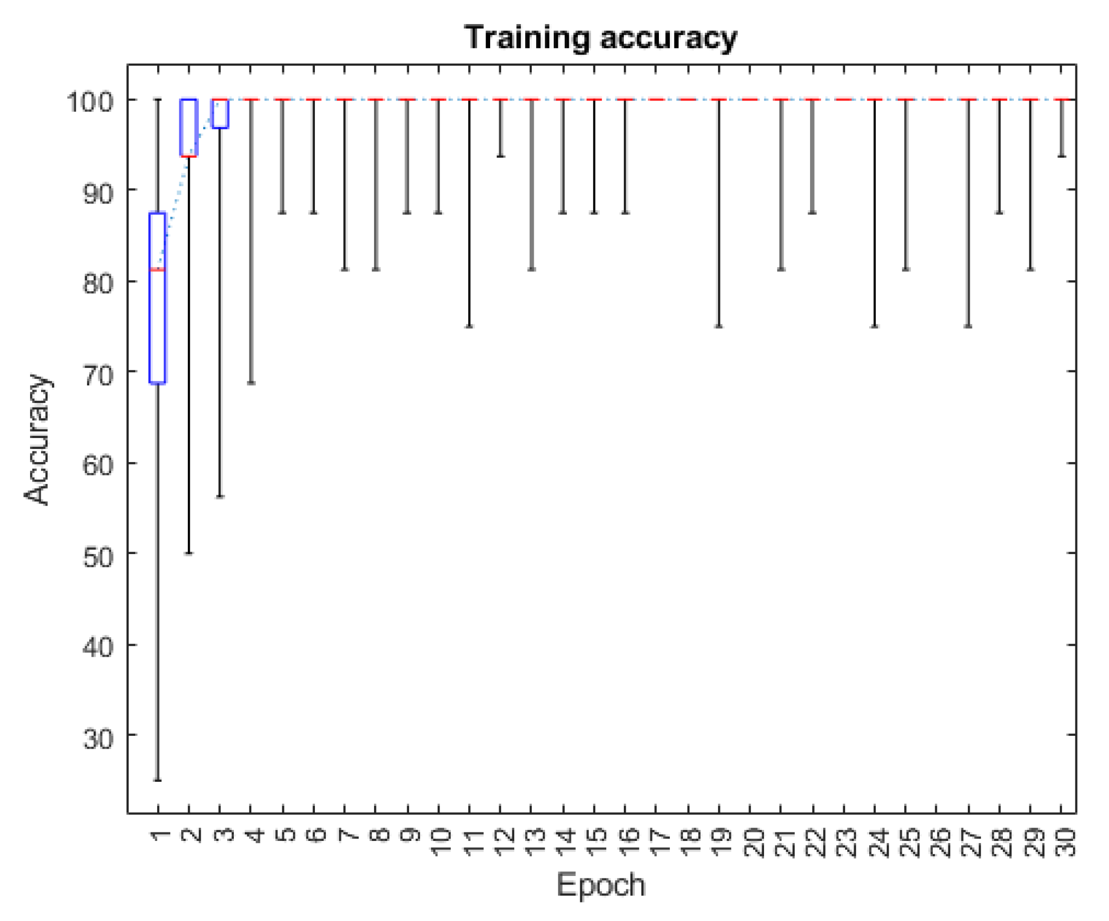
Under these conditions, the ResNet managed to achieve high accuracy during the training phase with the simulated raw data, with several iterations exceeding 95% and up to 100% accuracy, as illustrated in
Figure 8.
After the training phase, the test data set composed of 1200 crops (600 ships and 600 sea crops) was used to check the final performance of the ResNet. This test phase was aimed to assess the performance of the ResNet with an independent set of simulated data not used in the training phase. All crops were correctly classified, reaching an overall accuracy of 100%. However, to provide a realistic and quantitative performance of the ResNet, further test phases were needed that also involved real data, as detailed in the following section.
3. Results
Our goal was to assess the ResNet performance by using both real and simulated ERS raw data. In this way, we were able to simultaneously evaluate the quality of our simulation model, as well as the performance of the trained ResNet in real scenarios.
3.1. Test with Single-Point Ship Simulated Data
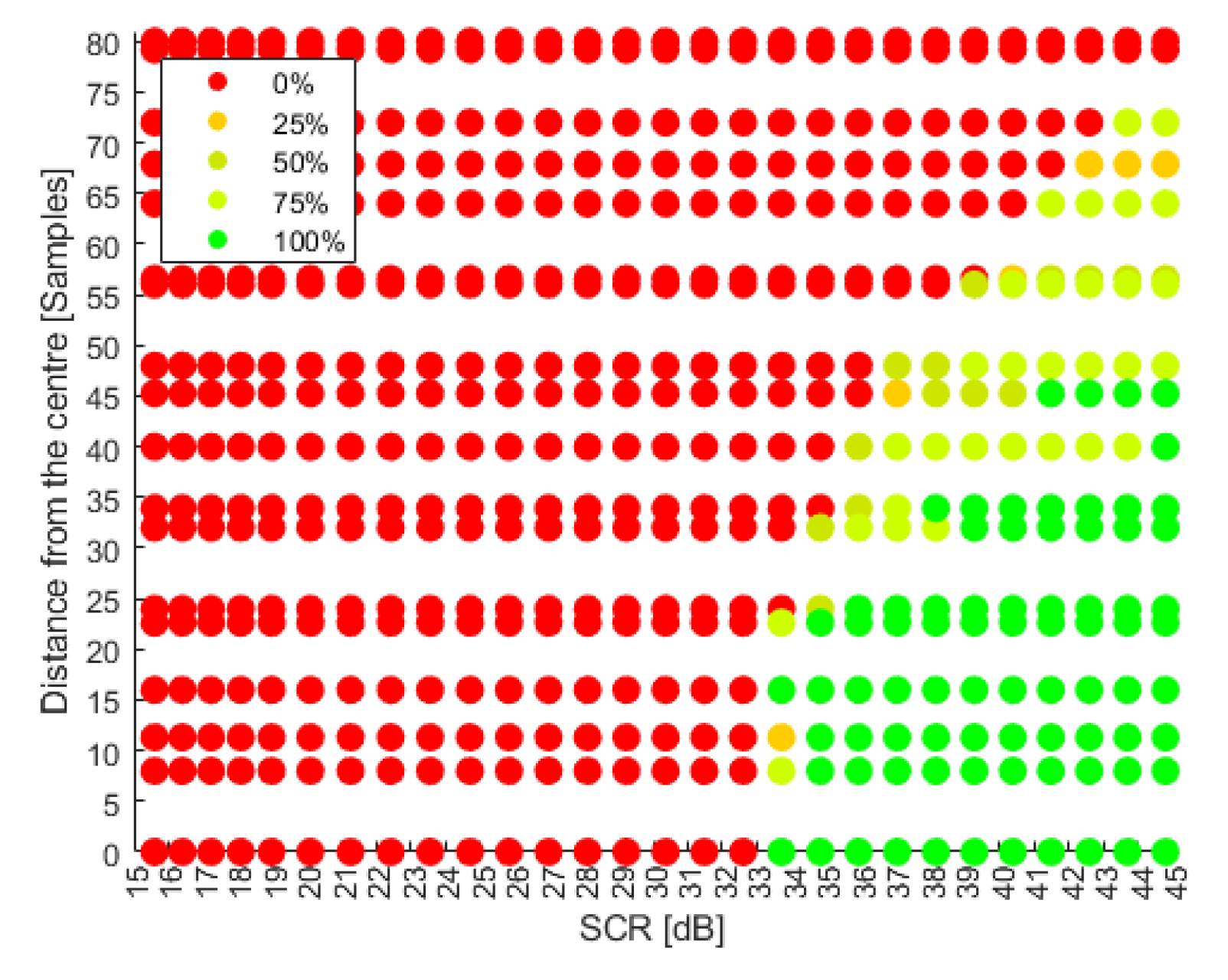
This test phase was aimed to assess the ResNet performance with another independent set of simulated data not used in the previous training and test phases. A single-point model for ship simulation was adopted with different conditions of SCR values and range/azimuth shifts. This gave us important insights into ResNet’s robustness and sensitivity to a wide range of conditions. More specifically, we investigated the detection performance as a function of SCR and shift values by further simulating 29 ship crops with an SCR varying from 15 to 45 dB. Starting from these simulations, we generated 2349 crops by applying a combination of 81 progressive azimuth and range shifts to the ship position with respect to the center of the crop. The size of the simulated crops is 100 × 100 samples in accordance with the training data set, while the range of ship positions was extended to ±80 samples and then more than 6 times higher than the ±12.5 range used in the training phase. This was conducted as a preliminary attempt to test the performance of the network beyond the limits it was trained with.
Under these conditions, we evaluated the ResNet’s classification result for each crop. The classification accuracy can be analyzed by means of the scatter plot presented in
Figure 9. It can be observed that the ResNet begins to detect the ship class with SCR > 33 dB. With higher SCR values, it is also able to tolerate a shift distance of <50 pixels with respect to the center of the crop.
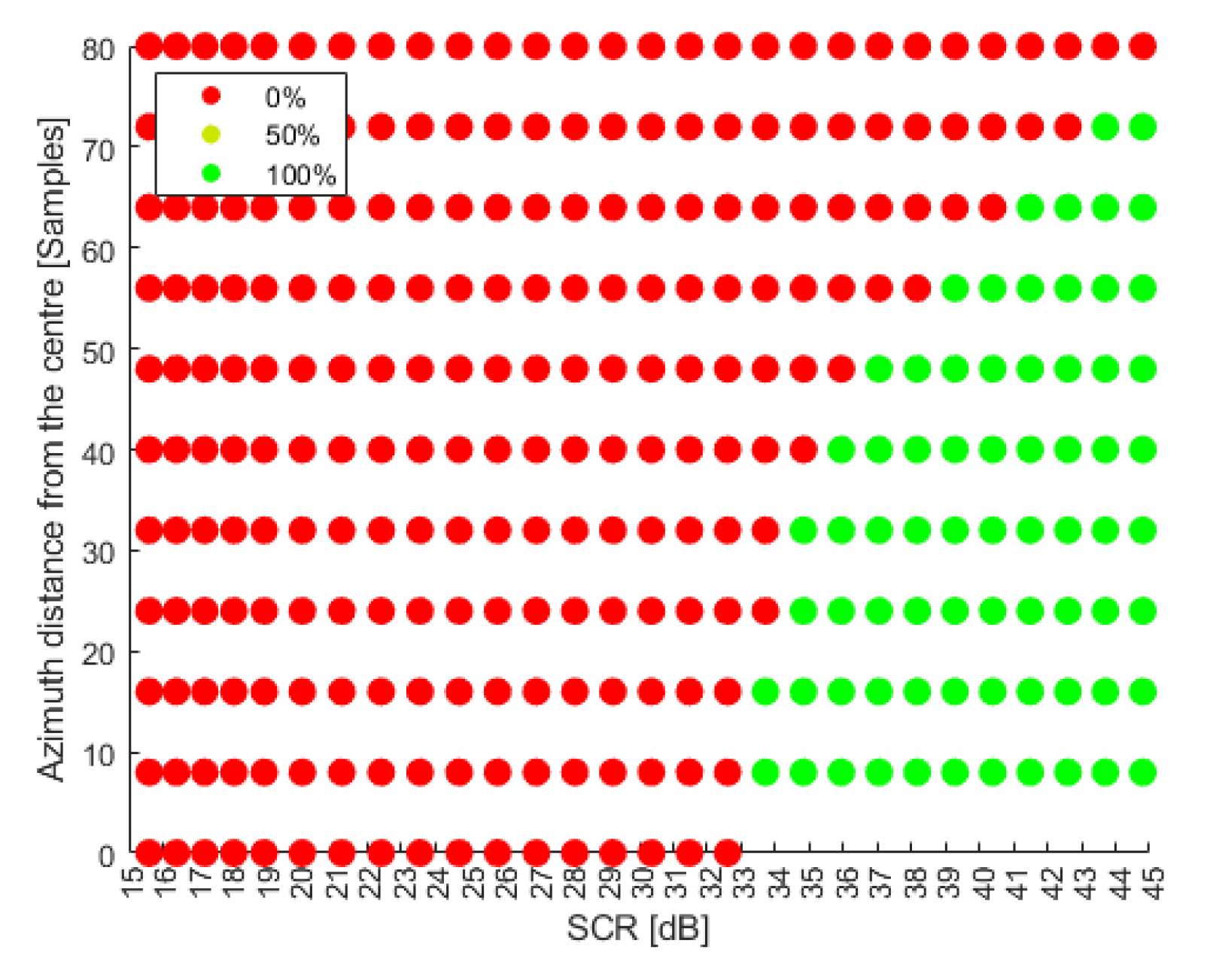
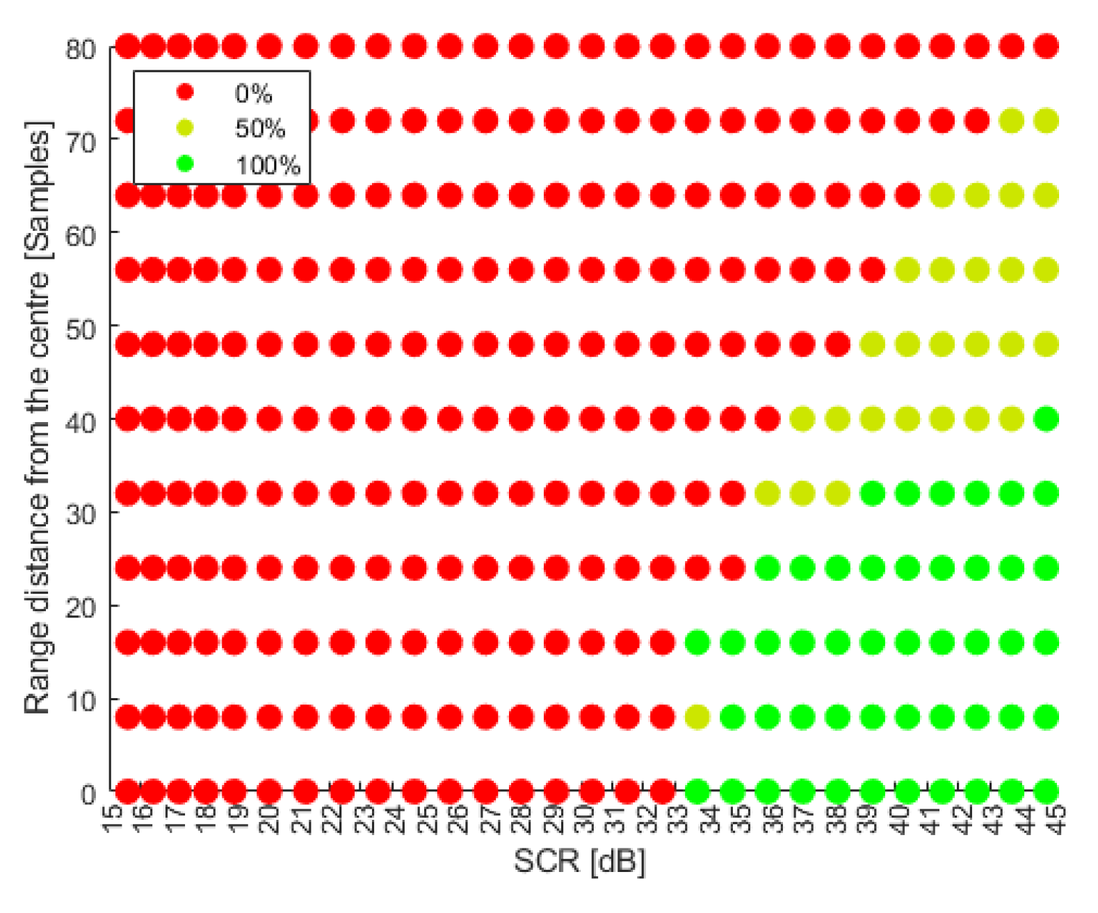
We also investigated the impact of the shift direction. Due to the different shapes of the impulse response along the azimuth and range directions, a different performance is expected when a ship shift is applied separately along these two axes. To this aim, scatter plots in
Figure 10 and
Figure 11 illustrate the classification accuracy when the shift to the ship position is applied in one direction only, with a zero shift in the other direction. The analysis of both plots shows that the proposed ResNet is more robust to azimuth shifts. This different performance will be further investigated in future works.
Finally, the performance related to false ship detection was evaluated. To this aim, 1000 crops containing only the SAR response of the sea were simulated with the same size as ship crops. The ResNet was able to correctly classify all the simulated crops, thus obtaining 100% accuracy in the detection of the sea class.
3.2. Test with Multi-Point Ship Simulated Data
The results obtained using the ResNet, in the case of single-point simulations, allowed us to confirm the ResNet’s ability to detect the presence of a ship using raw data. At first glance, the performance obtained in terms of the SCR may not appear particularly challenging. However, it should be considered that the resolution of the ERS data is equal to 5 m × 20 m, which means that the single-point response refers to very small vessels for which the literature is still exploring various solutions. Among the most promising approaches, we mention the use of multi-polarization sensors, which are not the subject of this analysis since the ERS mission operated exclusively in VV polarization. In this regard, in [
42], it is noted that in the case of small ships, the combined use of multiple polarizations leads to a detection capacity in the range between 38% (with the GNF method) and 85% (with the
method). In particular, the
method achieves the best performance with an SCR of 18.3 dB. However, the performances achieved by it do not correspond to single-point ships but always involve a limited extension of pixels, which can favor the application of SCR enhancement before detection.
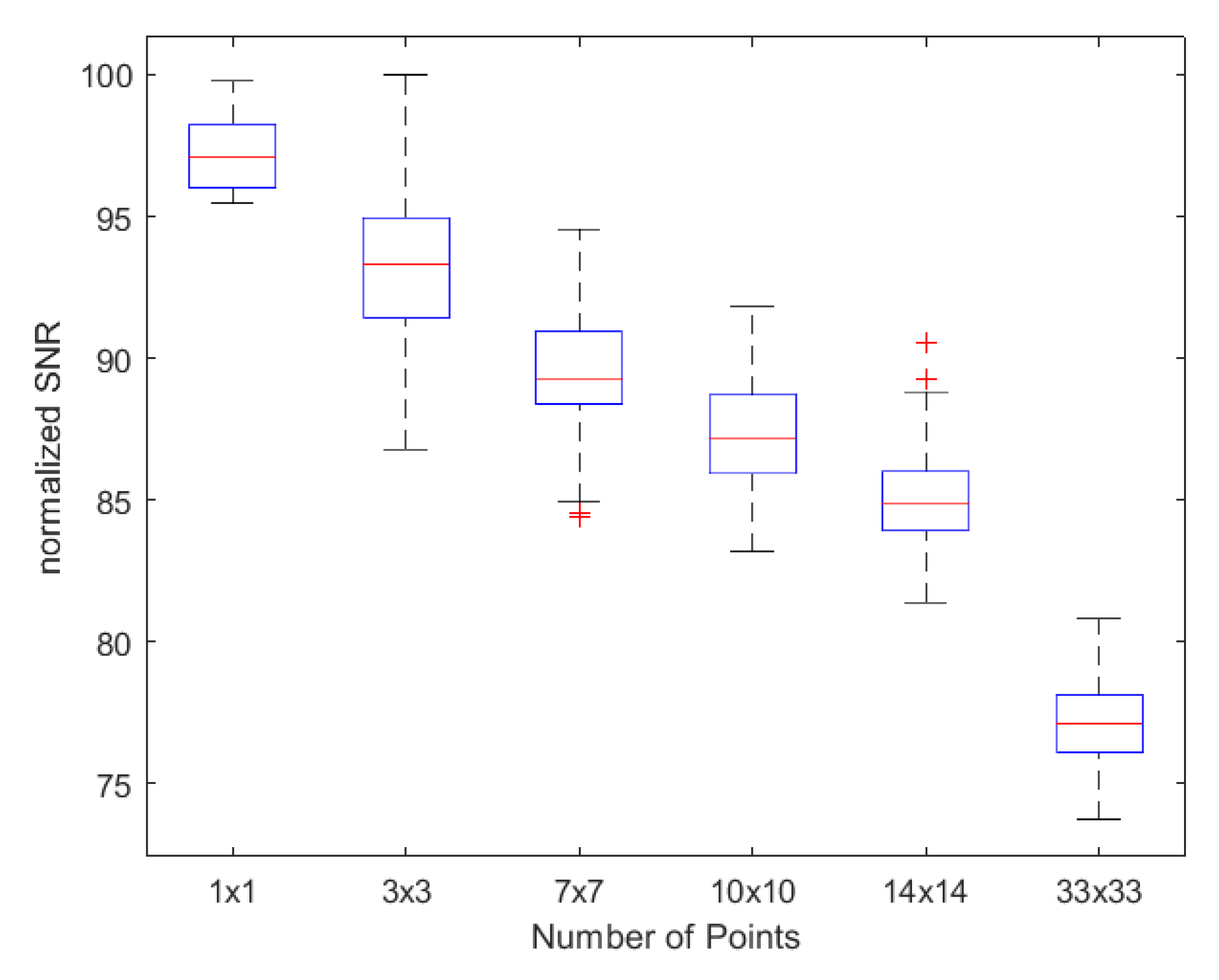
As observed, an analysis was, therefore, necessary to evaluate the impact of the extension of the ship on the performance of the detection algorithm. There are two contrasting aspects concerning this observation. First of all, it can be immediately observed that in the presence of several pixels associated with a ship, interference between the various responses is expected. This is confirmed via the graph illustrated in
Figure 12, in which it is evident that by increasing the number of pixels associated with a ship, there is a consequent drop in the SCR value.
However, the availability of more pixels per ship enables the generation of multiple echoes returned by the ship and, consequently, a greater overall energy received by the radar system.
In order to investigate how these two contrasting aspects impact the performance of the ResNet, several simulations were performed with ships having dimensions of 3 × 3, 7 × 7, 10 × 10, 14 × 14, and 33 × 33 pixels, corresponding to ground extensions of 15 × 60, 35 × 140, 50 × 200, 70 × 280, and 165 × 660 m. From an implementation point of view, it was sufficient to iterate the single-point simulator in different positions and sum the results in order to generate a multi-point ship radar response. Not all dimensions are realistic for a ship, but they have been taken into account to provide a sufficiently comprehensive picture of the ResNet’s performance in the case of a multi-point model.
It is observed that although the ResNet was trained with a single-point model, it was able to produce optimal performance when simulated ships have a size of 7 × 7 pixels. Under these conditions, it can be observed that the ResNet begins to correctly detect the ship class with SCR > 24 dB. With higher SCR values, it is also able to tolerate a shift distance of <60 pixels with respect to the center of the crop. This performance is well beyond the limits measured with a single-point ship simulation (resulting in an SCR > 33 dB and a maximum shift distance of <50 pixels). According to
Figure 13, it can be inferred that the 7 × 7-pixel size is a sort of sweet spot for ERS-based simulations. Beyond this size, the ResNet performance begins to decrease, probably due to the presence of pixels with a considerable inter-distance that introduces a strong deviation from the expected single-point ship impulse response used to train the ResNet.
3.3. Test with ERS Data
Finally, we conducted a thorough test of ResNet’s accuracy in ship classification using real ERS data. The first analysis consisted of verifying whether the performance measured on simulated data can be replicated on real data. To this aim, seven crops were extracted from ERS images corresponding to ships exhibiting an SCR between 24.8 dB and 40.1 dB. We applied to each crop progressive shifts to ship positions spanning ±80 samples along the azimuth and range directions. The results are illustrated in the scatter plot of
Figure 14, where it is also indicated the size in pixels of each ship in order to analyze the impact of this parameter on the ResNet detection accuracy. In particular, it is observed that the ResNet begins to operate correctly starting from an SCR equal to 26 dB.
It is possible to compare these performances with previous works available in the literature. To this aim, it was necessary to estimate the SCR values by computing the P
parameter as the average power of all the pixels belonging to the ship, obtaining the correspondences indicated in the
Table 6.
It is observed that the use of the average power in Expression (
14) significantly reduces the estimated SCR values. In particular, it is observed that the network begins to work correctly starting from an SCR
of 10.3 dB. This is in agreement with the results reported in [
44], where it is observed that the CFAR algorithm reaches a detection capability of 29.6% with an SCR
of 5.7 dB and of 81.6% with an SCR
of 10.9 dB.
The performances of the ResNet with real data also exhibit several points of good agreement with those measured in the simulation phase by means of the scatter plots of
Figure 13. More specifically, we observed the following:
- -
The ship with an SCR equal to 24.8 dB (having a size of 56 pixels) was not correctly detected via the ResNet. This is in good agreement with the performance measured with the 7 × 7-pixel ship simulation.
- -
The ship with an SCR equal to 30.8 dB (having a size of 110 pixels) was correctly detected via the ResNet with shifts lower than 40–45 pixels. This is in good agreement with the performance measured with the 10 × 10-pixel ship simulation.
- -
The ship with an SCR equal to 34.0 dB (having a size of 240 pixels) was correctly detected via the ResNet with shifts lower than 40 pixels. This is in acceptable agreement with the performance measured with the 14 × 14-pixel ship simulation.
- -
Even with the real data, there is some evidence of a potential sweet spot in the optimal ship size. In the case of the simulated data set, a 7 × 7-pixel sweet spot was identified. The reduced set of real data did not allow us to perform an exact estimation of the sweet spot; however, there are some practical considerations that lead us to infer that it should be positioned close to the one identified in the simulation phase. In particular, the following can be observed: (1) the ship with a size of 110 pixels and an SCR equal to 30.8 dB achieves the ResNet classification performances of the ship with an SCR equal to 34 dB, which has a larger size (240 pixels); (2) the two ships with similar SCR values (37.3 dB and 37.8 dB) exhibit very different performances, showing that the ship with a smaller size (100 pixels) has better performance than the ship with a 400-pixel size.
This confirms that our multi-point ship simulation methodology accurately represents the main characteristics of real ships and their interactions with clutter. Furthermore, this successful test with real data also confirms the validity of our single-point ship simulation approach for generating the simulated data, and it proves suitable for making the ResNet operative on real data.
However, the test with real data reveals some deviations in ResNet performance compared to that obtained with simulated data. In particular, it is not well understood why the real ship with an SCR equal to 26 dB exhibits better performances than those measured with simulated data. Future works will allow us to identify these anomalies.
Further analyses were instead conducted regarding the behavior of the ResNet with real data as a function of the direction of the shifts applied to the position of the ship with respect to the center of the crop. More specifically,
Figure 15,
Figure 16 and
Figure 17 show crops of ERS images extracted from three ships with different SCR values. For each crop, a graphic indication is provided on the shifts applied in the azimuth and range directions and the outcome of the classification corresponding to each shift. It is interesting to note the following:
- -
The detection accuracy associated with shifts applied along the azimuth direction is better than that relating to shifts along the range direction, and this is in agreement with what has already been observed in the simulation;
- -
The impulse response of the ship is visually recognizable only in the raw data associated with the third case (SCR, 40.1 dB), while with lower SCR values, this response is not visible, although the ResNet still demonstrates the capability to recognize the presence of the ship. Furthermore, this motivated why visual attention techniques were not considered in the first feasibility analysis.
Finally, similarly to what was performed in the simulation, the performance related to false ship detection was evaluated. To this aim, 3712 crops containing only the SAR response of the sea were extracted from ERS images. The ResNet returned only 40 false positives for an overall accuracy of 98.9%. A visual analysis of the input data associated with these wrongly classified crops did not allow us to identify any interesting clues that could motivate the wrong choices made via the ResNet (see
Figure 18). This prevented us from making changes in our tool for the simulation of sea crop data sets in order to improve the sea classification performance of the ResNet.
Furthermore, this highlights the limitations of present simulation methodologies in mimicking specific natural situations and the necessity for additional research and breakthroughs in simulating complicated marine settings for superior ResNet training and testing in ship detection applications. At the same time, this leads us to reconsider, in future works, the possibility of adopting a hybrid data set, including, within the simulated data set, real cases that the ResNet has not correctly classified.


 ,
, 


