A Novel Methodology for Classifying Electrical Disturbances Using Deep Neural Networks

Abstract

Electrical power quality is one of the main elements in power generation systems. At the same time, it is one of the most significant challenges regarding stability and reliability. Due to different switching devices in this type of architecture, different kinds of power generators as well as non-linear loads are used for different industrial processes. A result of this is the need to classify and analyze Power Quality Disturbance (PQD) to prevent and analyze the degradation of the system reliability affected by the non-linear and non-stationary oscillatory nature. This paper presents a novel Multitasking Deep Neural Network (MDL) for the classification and analysis of multiple electrical disturbances. The characteristics are extracted using a specialized and adaptive methodology for non-stationary signals, namely, Empirical Mode Decomposition (EMD). The methodology’s design, development, and various performance tests are carried out with 28 different difficulties levels, such as severity, disturbance duration time, and noise in the 20 dB to 60 dB signal range. MDL was developed with a diverse data set in difficulty and noise, with a quantity of 4500 records of different samples of multiple electrical disturbances. The analysis and classification methodology has an average accuracy percentage of 95% with multiple disturbances. In addition, it has an average accuracy percentage of 90% in analyzing important signal aspects for studying electrical power quality such as the crest factor, per unit voltage analysis, Short-term Flicker Perceptibility (Pst), and Total Harmonic Distortion (THD), among others.

1. Introduction

Power generation systems comprise different levels: generation, distribution, transmission, and consumption [1]. Electrical energy monitoring, analysis, and quality are essential at all these levels and constitute the main challenges within these distribution, transmission, and consumption infrastructures. Monitoring and analyzing energy quality in real time is essential to subsequently apply the corresponding mitigation actions and not interrupt industrial or critical processes [2]. According to the IEEE 1159 standard [3] and European EN 50160 standard [4] electromagnetic phenomena that disturb electrical power quality in generation systems are called power quality phenomena or Power Quality Disturbances (PQDs). These two documents define the physical properties and characteristics of the PQDs and, in simple terms, define the PQDs as the deviation of voltage and current from their ideal sinusoidal shape. The intrinsic characteristics of these phenomena are attributed to elements such as intermittent power flow caused by the use of maximum power point tracking control and harmonic current injections caused by various power converters using type control techniques. With the introduction of necessary elements in the Industry 4.0 paradigm, the Internet of Things, and automatic manufacturing systems in these paradigms, many power converters based on high-frequency switching power electronic devices are necessary [5]. These phenomena or deviations severely affect the reliability and interoperability of industrial processes and electronic equipment. The negative impacts are diverse, including economic losses for the industries, such as effects on the distribution architecture and impact on the devices that consume the generated energy. The power quality problem has become increasingly prominent, so the main task is to guarantee voltage stability in power generation and distribution systems [6]. In this context, guaranteeing a high-quality power supply has become one of the tasks to be resolved urgently [7]. The architectures where the quality of electric power is most unstable are in microgrids because these types of schemes often use renewable distributed generators, which depend on natural resources [8]. Figure 1 shows an example of the architecture of microgrids.

Power quality in microgrids is a critical issue as it directly affects the efficiency and reliability of electricity supply [9]. Microgrids are designed to operate independently by integrating multiple types of distributed power generators, such as solar and wind, and storage systems with batteries and sometimes connected to the main grid [10]. Ensuring high power quality in a smart microgrid requires analyzing, quantifying, and monitoring the voltage signal, and the subsequent task of controlling and compensating for disturbances is necessary. The nature of microgrids as well as of electrical disturbances is stochastic [11]. PQDs not only occur individually but also occur in multiple or triggered manners. That is, it is common for frequency and voltage effects to occur jointly and randomly. The appearance of new combinations of PQDs means that monitoring and analysis schemes must be able to adapt and process new behaviors concerning already-known information [12]. As a result of this need, artificial intelligence has played an essential role in classifying and analyzing multiple PQDs. The methodologies proposed over the years have been diverse and innovative in feature extraction, classification strategies, difficulty levels, and learning methodologies. However, most of them face the dilemma of the stochastic and random behavior of PQDs. This work was carried out in the study, analysis, design, and development of a methodology necessary for classifying and analyzing the different electrical disturbances. The quantification of electrical disturbance is also performed to study the severity of the impact of electrical disturbances on the quality of electric power and facilitate studies in electrical energy. The main contributions of this work are as follows:

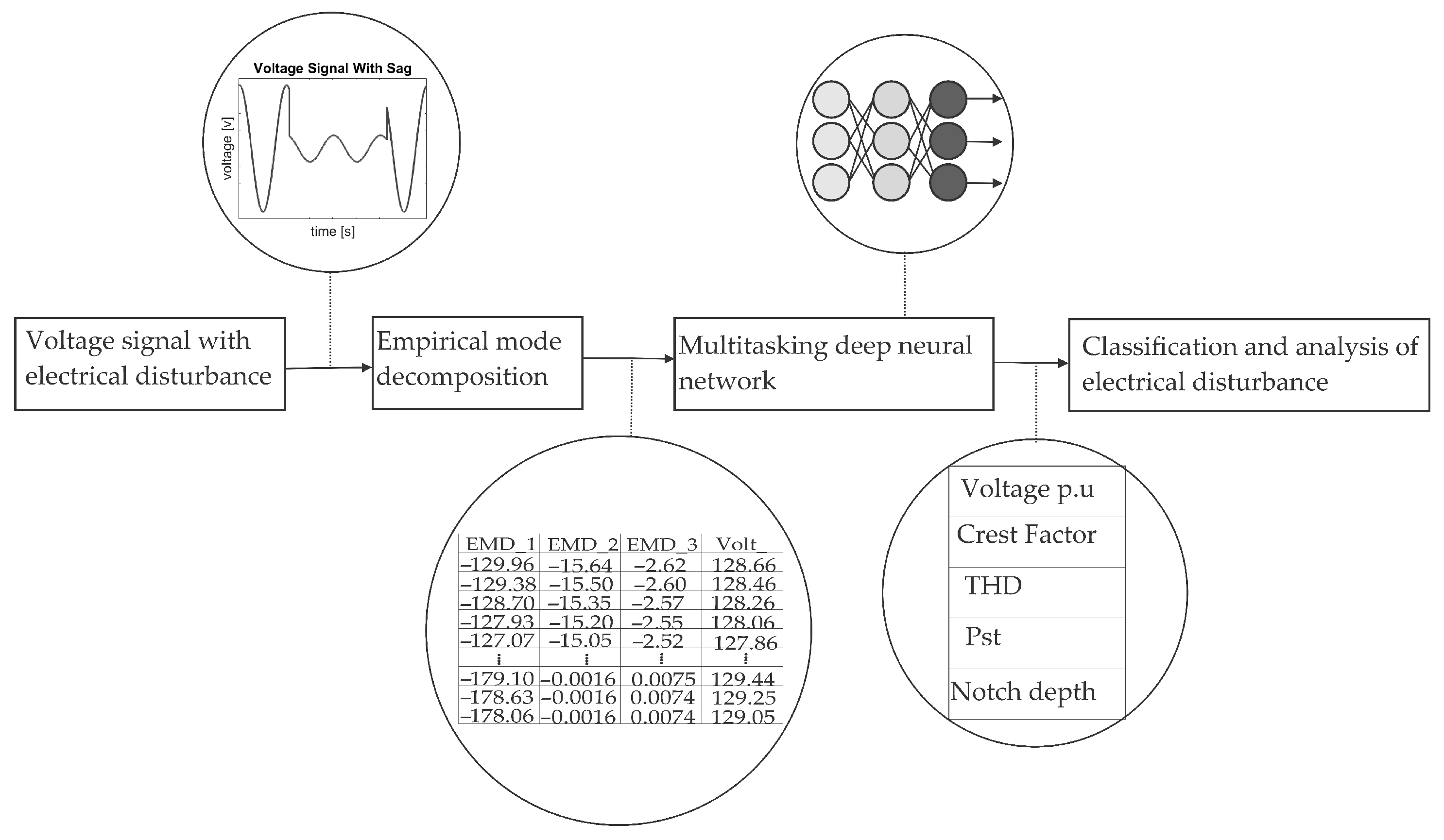
• This paper presents a novel multitasking deep learning model for classifying and quantification multiple electrical disturbances.
• This study proves how deep multitasking learning is an excellent model for solving the challenge of quantitative analysis and classification of multiple electrical disturbances without the level of complexity or noise in the signal being a problem.
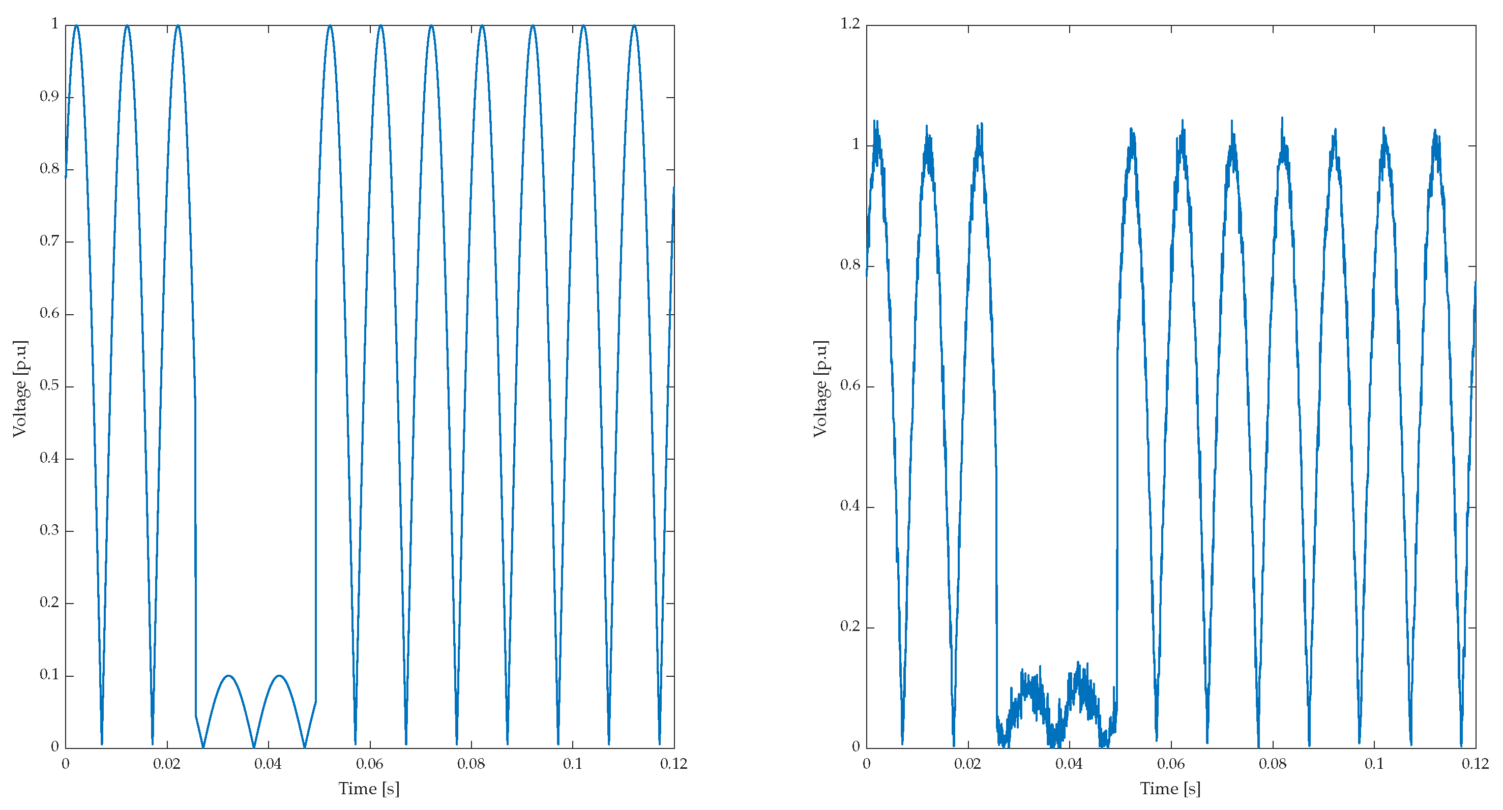
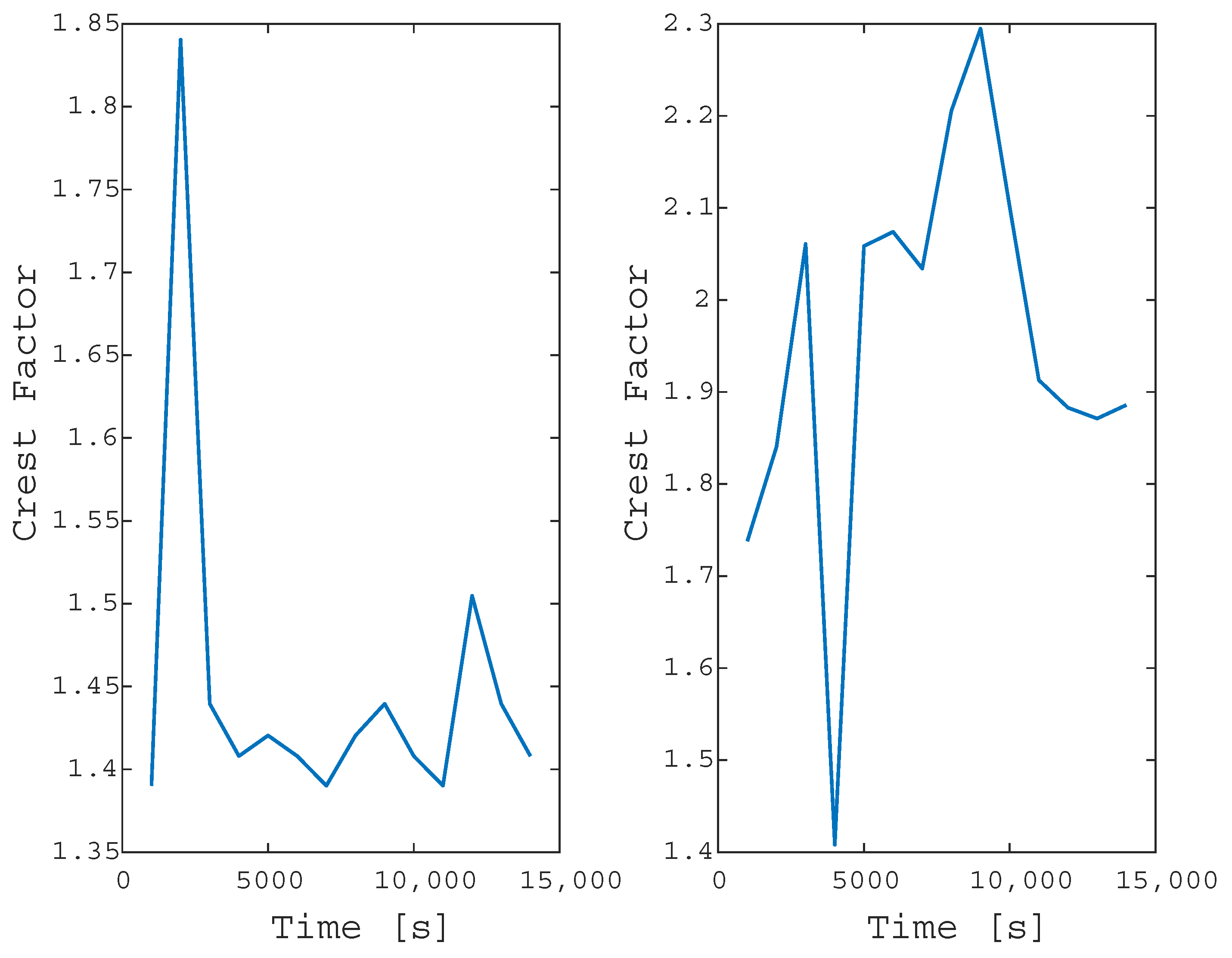
• Graphs are shown where the assessment of the quality of electrical power with electrical disturbance can be observed. This way, assessing the quality and impact of linear and linear loads is simpler.
• The extraction of characteristics is proposed using an adaptive oscillatory methodology. Due to the random nature of the electrical disturbances, this paper proves how using traditional strategies presented in other articles is ineffective.
• The development and testing were conducted with 29 electrical disturbances, from single disturbances to several simultaneous electrical disturbances, with noise levels ranging from 20 dB to 50 dB.
• The development of additional tests performed on an island network with a photovoltaic system and high-switching elements is described. In addition, electrical disturbances of all 29 levels with noise levels between 20 dB and 50 dB were constantly injected.

The organization of the article is as follows: Section 1 presents the introduction. Section 2 presents briefly the main contributions and methodologies proposed by several authors in the monitoring and processing of electrical disturbances. Section 3 presents the theoretical background, Section 4 the materials and methods, Section 5 the analysis and results, and finally, Section 6 concludes this work.

2. Related Works

Table 1. Comparison of methodologies in multiple electrical disturbances.

Paper	Year	Feature Extraction Methodology	Signal Classification Methodology
[13]	2018	Initial layers in the neural network	Deep neural network
[14]	2019	One-dimensional convolutional, pooling, and batch normalization layers to capture multi-scale features	Closed-loop deep-learning method
[15]	2019	Empirical wavelet Transform-based adaptive filtering technique	Multiclass support vector machine (SVM)
[16]	2019	Root Mean Square, Skewness, Range, Kurtosis	Improved Principal Component Analysis (IPCA) and 1-Dimensional Convolution Neural Network (1-D-CNN)
[17]	2020	Initial layers in the neural network	Long Short Term Memory (LSTM), Convolutional Neural Networks (CNN), Convolutional Neural Networks Long Short Term Memory (CNN-LSTM), and CNN-LSTM
[18]	2020	Global power quality indices (GPQIs)	Cluster analysis (CA)
[19]	2021	Stockwell Transform	Extreme Learning Machine (ELM)
[20]	2021	Discrete Wavelet Transform	Model assembled with Logistic Regression (LR), Naïve Bayes, and J48 decision tree
[21]	2021	Discrete Wavelet Transform and adaptive salp swarm algorithm	Probabilistic neural network
[22]	2022	Hilbert Transform and Wavelet Transform	Support Vector Machine
[23]	2022	Discrete Wavelet Transform	Artificial Neural Network

presents some relevant contributions in aspects such as feature extraction methodology and signal classification methodology. It shows a great diversity of methodologies but also, at the same time, a clear trend for the classification of electrical disturbances. Phases such as the extraction of signal characteristics, classification methodologies, and the type of output of the neural network are detected in these contributions. Within the first phase of feature extraction, researchers traditionally use strategies such as Discrete Wavelet Transform, Hilbert Transform, S-Transform, power quality indices, statistical signal characteristics, deep neural network layers, discrete Fourier Transform, Fast Fourier, etc. These are good strategies for working with signals and for analyzing and extracting information. PQDs possess an intrinsic nature of behaving as non-linear and non-stationary signals. Due to this, the methodology for extracting characteristics is a vital phase for the algorithm because it will be the input values of our signal analyzer and classifier algorithm. The Discrete Wavelet Transform (DWT) is based on wavelets, which are mathematical functions that efficiently represent the characteristics of a signal. The Wavelet Transform (WT) extracts information in time and frequency domains, suitable for dynamic signals, but it needs help when the data is noisy, as its level of precision drops considerably. Discrete Fourier Transform (DFT) and Short Time Fourier Transform (STFT) are elements of low computational consumption, but they have problems analyzing and detecting frequency phenomena. Stockwell Transform (St) is a combination of STFT and WT, whereby it has a better extraction and characterization of the signals; however, it is a redundant representation of the time-frequency domain, and its processing time is longer if the sampling time increases. Using statistical strategies or power quality indices as important signal characteristics is a good strategy. However, the learning algorithm needs precise characteristics of the types of signals, and these types of quantifiable values can have a considerable level of variability between types of signals. In addition, feature extraction methodologies often generate information that can cause problems due to the amount of information generated that is only sometimes significant; as a result, multiple authors implement algorithms such as Principal Component Analysis, LDA, or metaheuristic algorithms. Due to the nature of electrical disturbances being non-linear and non-stationary signals, the methodology becomes more complex and, to some extent, with overfitting and precision problems.

Another critical point is the development of models which can observe a great diversity among the strategies, most residing in neural networks, varying between simple networks or deep networks. Softer strategies such as support vector machines, Logistic Regression (LR), Naïve Bayes, and J48 decision tree are also presented. The output of each of these models is a variable or label which determines the type of electrical disturbance; that is, the output is traditionally a label such as “Sag” or “Swell”. All these methodologies solve the electrical signal classification task by only determining the taxonomy of the multiple PQDs from different classification and feature extraction perspectives. However, this does not mean that the taxonomy is the only element for the proper monitoring of the quality of electrical energy. The analysis of the signal and the quantification of essential values to assess the severity of the disturbance are scarce characteristics in this type of contribution. As a result of this need being detected within electrical power quality monitoring systems in this context, this paper proposes a novel methodology, namely, a multitasking deep neural network for the classification and analysis of multiple electrical disturbances with the capacity to process, analyze, and classify signals, not stations, for the in-depth study of the quality of electrical energy. In addition, the design, development, and the different tests are carried out with about 29 difficulty levels and a data set with high diversity in time parameters and severity of electrical disturbances as well as various noise levels in a range of 10 dB up to 50 dB. The performance quantification shows an accuracy above 98% in the training, validation, and test phases. Performance tests were carried out in different scenarios of power generation systems with different configurations and levels of complexity.

3. Theoretical Background

Developing a system monitoring electrical power quality has been a potential development area in recent years. This section presents the essential elements for developing the classification, analysis, and monitoring proposal described in this paper.

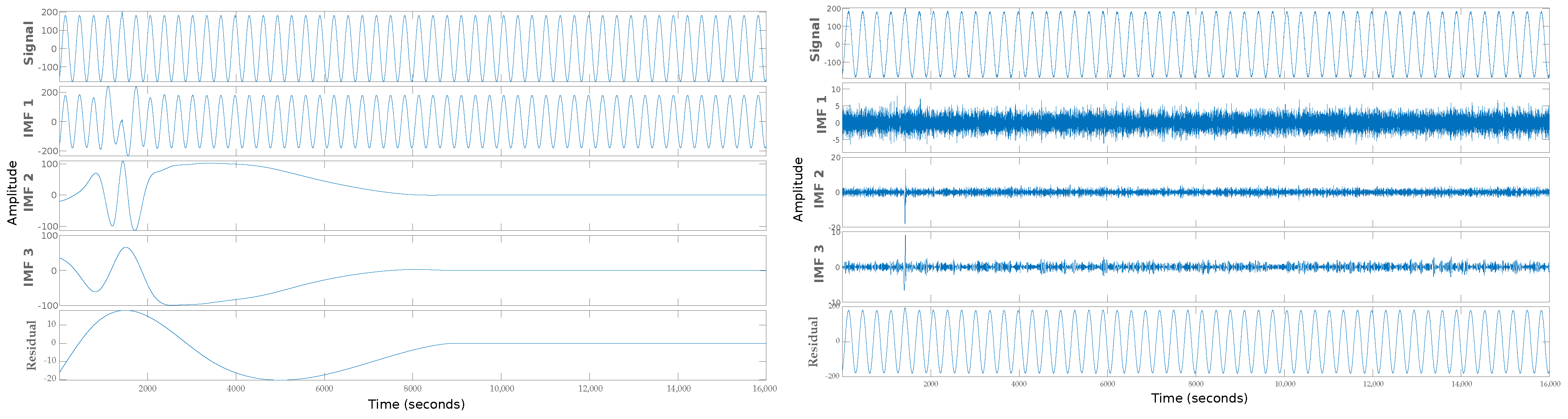
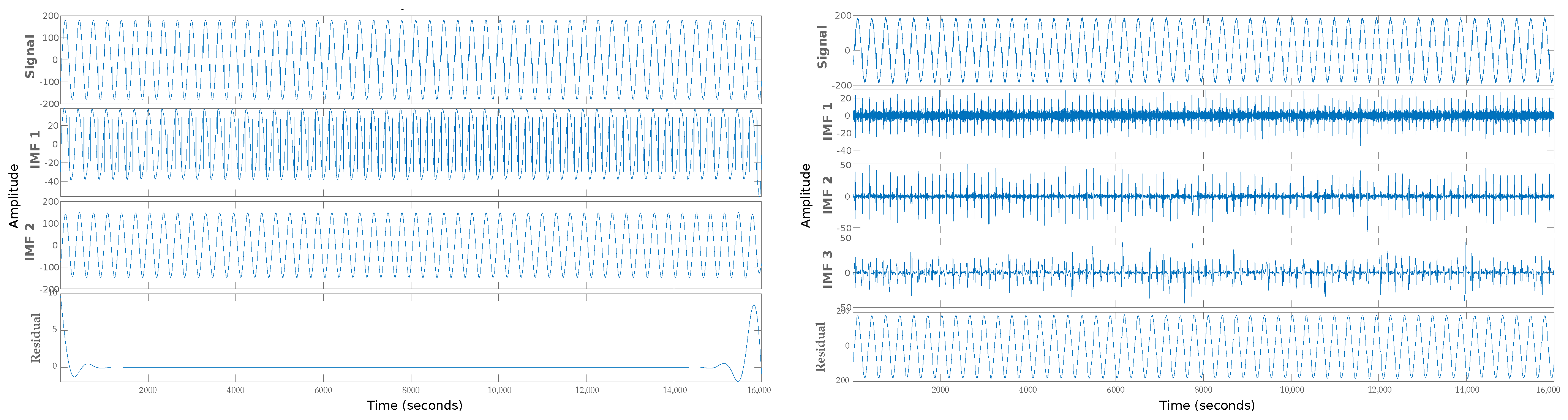
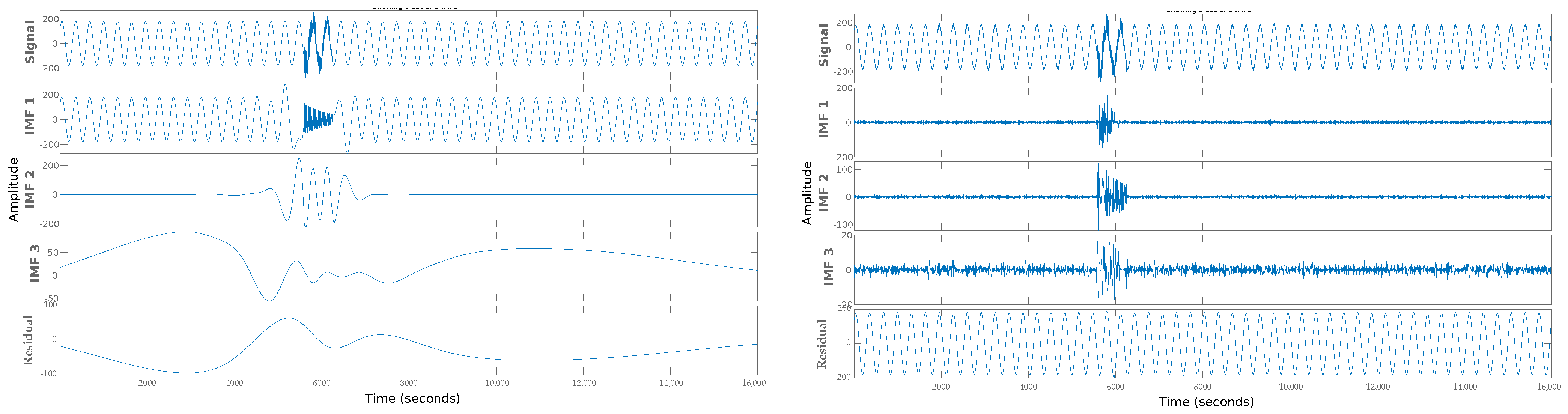
3.1. Empirical Mode Decomposition

Empirical Mode Decomposition (EMD) is a data analysis method used in signal processing and time series analysis. It is a non-linear and non-stationary signal processing technique that decomposes a signal into its underlying oscillatory components, called Intrinsic Mode Functions (IMF). The EMD method is based on the concept of “mode”, which refers to a quasi-periodic oscillation that can be extracted from a signal. EMD uses a sifting process to isolate these IMF by repeatedly decomposing a signal into high and low-frequency components until the residual is a monotonic function [24]. The process is as follows:

• Initialize the signal $x(t$) to be decomposed into a set of intrinsic mode functions (IMF).
• For each IMF component $i(i=1,2,\dots ,N)$, repeat the following sifting process until convergence:

  (a)

  Identify all local maxima and minima of $x\left(t\right)$ to obtain the upper and lower envelopes, respectively.

  (b)

  Calculate the average of the upper and lower envelopes to obtain the mean envelope $h\left(t\right)$.

  (c)

  Subtract the mean envelope $h\left(t\right)$ from the signal $x\left(t\right)$ to obtain a “detrended” signal $d\left(t\right)$.

  (d)

  Check whether $d\left(t\right)$ is a valid IMF by verifying the following conditions:

  • The number of zero-crossings and extrema must be equal or differ at most by one.
  • The local mean of $d\left(t\right)$ is zero.

  (e)

  If $d\left(t\right)$ satisfies the above conditions, it is considered an IMF, and the sifting process for this IMF is complete.

  (f)

  If $d\left(t\right)$ does not satisfy the above conditions, it is added to the residual signal, and the sifting process is repeated on the residual signal.

• The residual signal obtained after sifting all IMF is the final trend component of the signal.

The EMD algorithm is an iterative process that extracts the oscillatory components of the signal by sifting out the trend component at each iteration. The resulting IMF are typically sorted in order of decreasing frequency, with the first IMF representing the highest frequency oscillation in the signal. The EMD algorithm can be computationally intensive and may require careful tuning of parameters to achieve accurate decomposition [25].

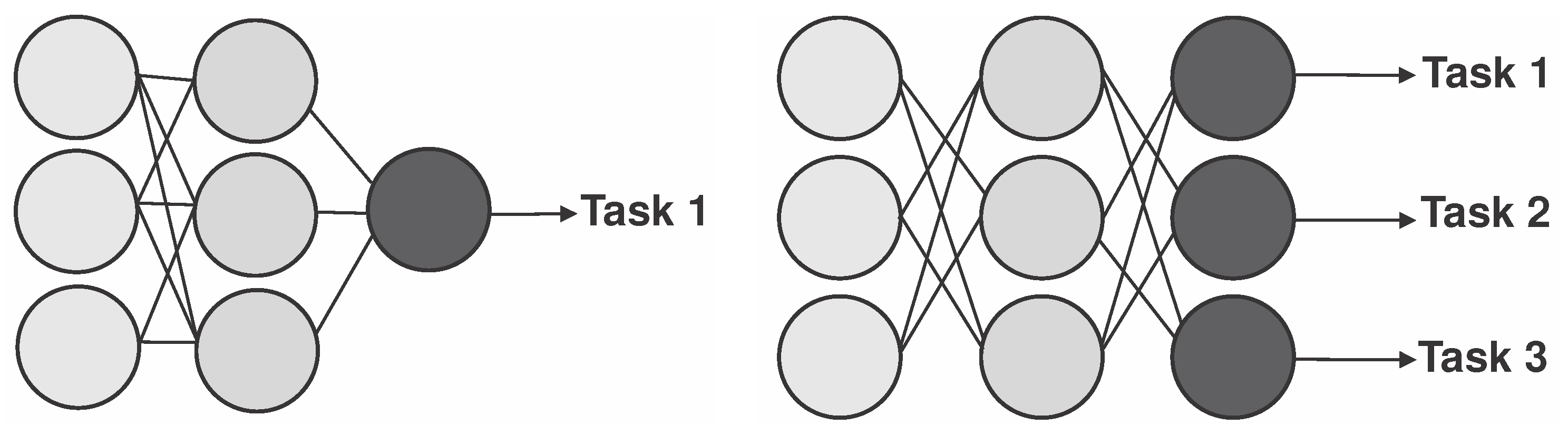
3.2. Multitasking Deep Neural Network

Learning paradigms within deep learning and machine learning, such as supervised learning, offer fast and accurate classification and regression solutions in various intelligent systems and real-world applications [26]. The traditional methodology of learning paradigms is to learn a function that maps each given input to a corresponding output [27]. For classification problems, the output is a label or an identifier character. For data regression problems, it is a single predictive value, such as temperature or amount of money. A traditional learning paradigm is an excellent tool for solving various problems; however, sometimes, it needs to adapt better to the growing needs of today’s complex decision making [28]. From this arises the pressing need to develop learning paradigms, and thus emerged multi-head neural networks or multi-head deep learning models, also known as Multi-output Deep Learning models (MLD). MLD takes advantage of the relationship between tasks to improve the performance of learning models [29]. Figure 2 compares the architecture of a traditional deep neural network and an MLD.

Figure 2 is an example of how MLD works in images. This methodology can detect and classify elements in an image that could be undetectable to the human eye. It is essential to mention that MLD is widely used in medicine and has good performance results. In [29], MLD is used for surgical assistance in analyzing surgical gestures and predicting the progress and status of surgical movements. MLD has also been applied to determine ship positions in the contribution of [30]; the authors analyze satellite images to detect multiple ship positions and determine the position coordinates in case the ship sensors fail and have to track ships with industrial containers. Deep learning multitasking refers to the ability of a deep learning model to perform multiple tasks or learn multiple functions simultaneously. The model is trained to perform more than one task, such as image classification and object detection or natural language processing. Deep learning multitasking can have several advantages, including improved performance on each task, reduced training time and computational resources, and the ability to learn shared representations that can benefit all tasks. It can also be more robust to noisy or incomplete data, as it can leverage information from multiple sources.

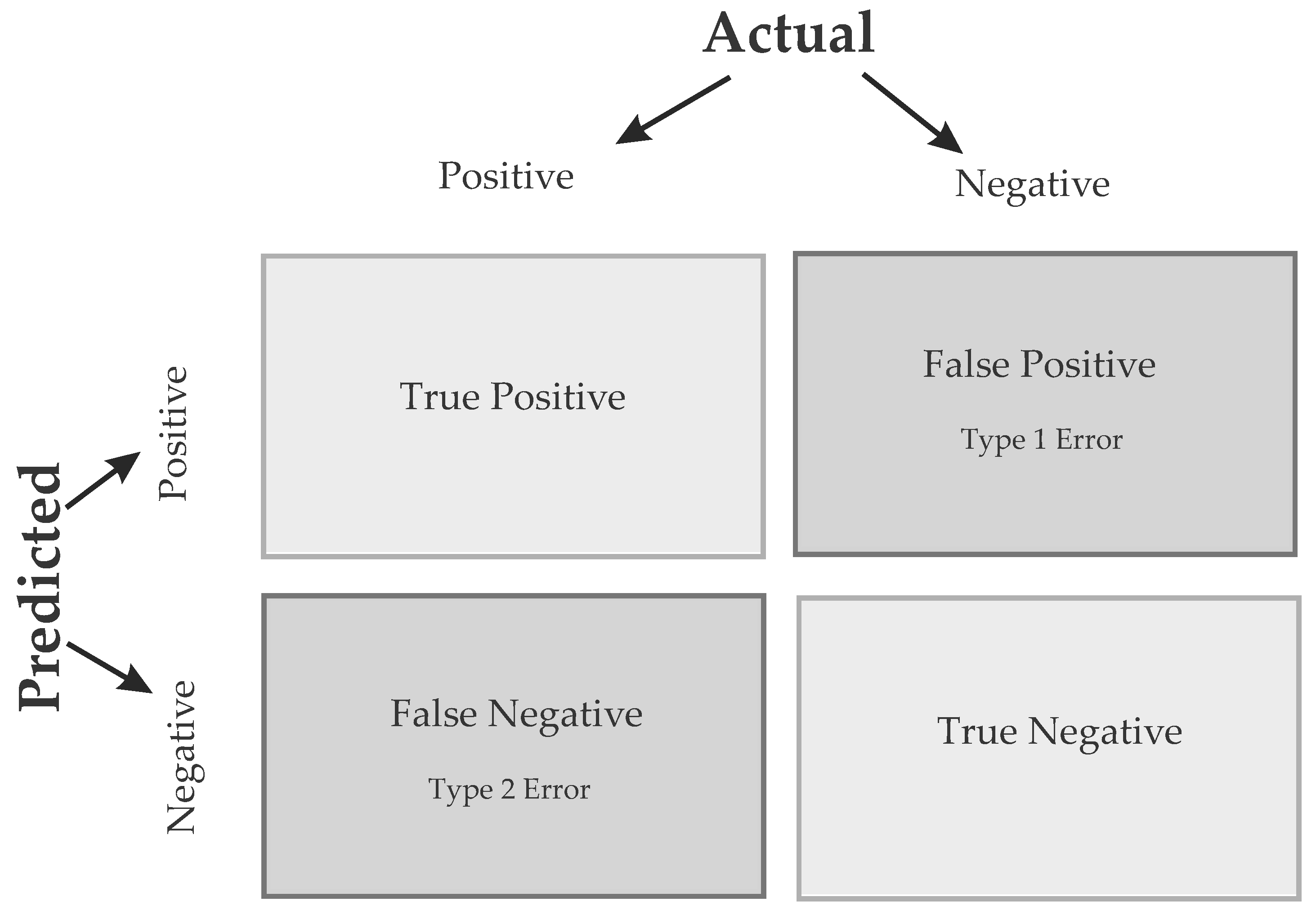
3.3. Performance Indices

The performance indices are elements used to quantify the behavior of the proposal in this work at different levels of complexity of PQDs and electrical generation systems with different architectures or scalability.

Table 2. Performance indices for data prediction.

Performance Indices	Formula	Meaning of Symbology
Mean absolute error	$MAE=\frac{1}{N}{\sum }_{i=1}^N|y_i-y_p|$	$y_p$ is the predicted value $y_i$ is real value N is the total number of data
The absolute mean percentage error	$MAPE=\frac{1}{N}{\sum }_{i=1}^{N}100\frac{|y_i-y_p|}{y_i}$	$y_p$ is the predicted value $y_i$ is real value N is the total number of data

shows the PQDs analysis, quantification, and regression task indices.

For the task of classifying PQDs by labels, indices were used, which are aided by the Confusion Matrix (CM) shown in Figure 3. A CM is a table that evaluates a classification algorithm’s performance for a classification problem. It compares the predicted class labels to the actual class labels of a data set.

The rows of the CM represent the actual class labels, while the columns represent the predicted class labels. The CM main diagonal represents the correctly classified samples, while the off-diagonal elements represent the misclassified samples. A CM typically has four entries:

• True positives (TP): Corresponds to the samples correctly predicted as positive.
• False positives (FP): Corresponds to the incorrectly predicted as positive.
• True negatives (TN): Corresponds to the correctly predicted as negative.
• False negatives (FN): Corresponds to the incorrectly predicted as negative.

The CM provides the valuable information of a classification algorithm, such as accuracy, precision, recall, and F1-score. The

Table 3. Performance indices for data classification.

Performance Indexes	Formula
Accuracy	$Accuracy=\frac{TP+TN}{TP+TN+FP+FN}$
Recall	$Recall=\frac{TP}{TP+FN}$
Specificity	$Specificity=\frac{TN}{TN+FP}$

shows the formulas for these characteristics to determine the performance of a classification algorithm.

4. Materials and Methods

Figure 4 shows the methodology used to analyze and classify the different levels of complexity of electrical disturbances.

First, there is the electrical disturbance generation block. In later sections, the nature and properties of the different electrical disturbances throughout the proposal of this paper will be described in more detail. The second block corresponds to the extraction phase of the characteristics of the different electrical disturbances with the algorithm of empirical decomposition, which breaks down into Intrinsic Mode Functions (IMF). The first three IMF for electrical disturbances are recommended since they have more relevant information. The first two components contain high frequencies, and the third is information related to disturbances in the fundamental component. Further, this is implemented to lower computational consumption time and fast response. In addition to these values, the voltage value of the electrical disturbance is added. These values form a matrix comprising the three IMF columns and the voltage value of the signal, which are the input values of the Multitasking Deep Neural Network system. Subsequently, when introducing these values to the architecture of the Multitasking Neural Network, it processes them. In later sections, the architecture and components of this multitasking deep neural network will be discussed in more detail. The output of the neural architecture presents a vector that is composed of two groups of fields. The first is a numerical identifier of the type of disturbance that goes from 1 to 29; later sections will explain what assignment each of these has numbers. The other group of values is an essential element for the analysis and quantification of the quality of electrical energy, that is, to evaluate the quality in amplitude and frequency. These elements include voltage per unit, the crest factor, Total Harmonic Distortion (THD), Short Term Flicker Perceptibility (Pst), notch area, and depth.

4.1. Synthesis of Electrical Disturbances and Database

The electromagnetic phenomena used to test and develop the Multitasking Deep Neural Network model were made synthetically. Developing a synthesizer system of multiple electrical disturbances was carried out, the physical characteristics of which vary. However, the voltage signal without electrical disturbances has the following characteristics show in

Table 4. General characteristics of synthesis of electrical disturbances.

Parameter	Value
sample rate	16 kHz
Peak Voltage	180 V
Frequency	60 Hz

.

The synthesis of the different levels of electrical disturbances was based on different mathematical models, which are presented in Appendix A; these mathematical models are the scientific contribution of [31], and each electrical disturbance has different characteristics individually, such as duration time, disturbance severity characteristics such as p.u voltage rise or voltage loss, among other characteristics used in mathematical models for their correct synthesis.

Table 5. Fragment of the table in Appendix A of mathematical models of electrical disturbances.

Power Quality Disturbance	Identifier	Mathematical Model	Synthesis Parameters
Normal Signal	1	$v\left(t\right)=180sin(\omega t-\varphi )$	$\omega =2\pi \ast 60\frac{rad}{s}$
Sag	2	$v\left(t\right)=180(1-\alpha (u(t-t_1)-u(t-t_2)))sin(\omega t-\varphi )$	$0.1\le \alpha \le 0.9$
Swell	3	$v\left(t\right)=180(1$+$\beta (u(t-t_1)-u(t-t_2)))sin(\omega t-\varphi )$	$0.1\le \beta \le 0.9$

shows a fragment of the table in Appendix A with the first five levels of types of electrical disturbances. This table shows essential fields such as the name of the electrical disturbance and the numerical identifier, which is used as one of the output parameter elements of the Multitasking Deep Neural Network model. This identifier is associated with the level of complexity of the electrical disturbance. The table in Appendix A shows 29 different levels, where the complexity increases as the value of the identifier increases.

Table 5 shows the mathematical model of the electrical disturbance, which was used to synthesize the multiple electrical disturbances and used in the development of the model and the different performance tests. Different parameters are shown in all formulas for electrical disturbances, such as the duration time where t is the total time, the parameter $t_1$, and the parameter $t_2$, which is the end of the electrical disturbance. Moreover, they have different synthesis parameters that represent the severity of the electrical disturbance. These values are determined randomly to have a diverse data set to develop the Multitasking Deep Neural Network model better. In addition, this multiple electrical disturbance synthesis system developed a data set for the training, validation, and testing of the Multitasking Deep Neural Network models. About 5000 different electrical disturbances were synthesized in the aspects of disturbance duration time, severity of electrical disturbance, and synthesis parameters; the only fixed value is sampling frequency, with a value of 16 kHz. In this way, 70% of the data set was used for training, equivalent to 3500 electrical disturbances, and 15% for the validation and test phases, the equivalent of 750 disturbances of the 29 levels of electrical disturbances with a great variety of syntheses.

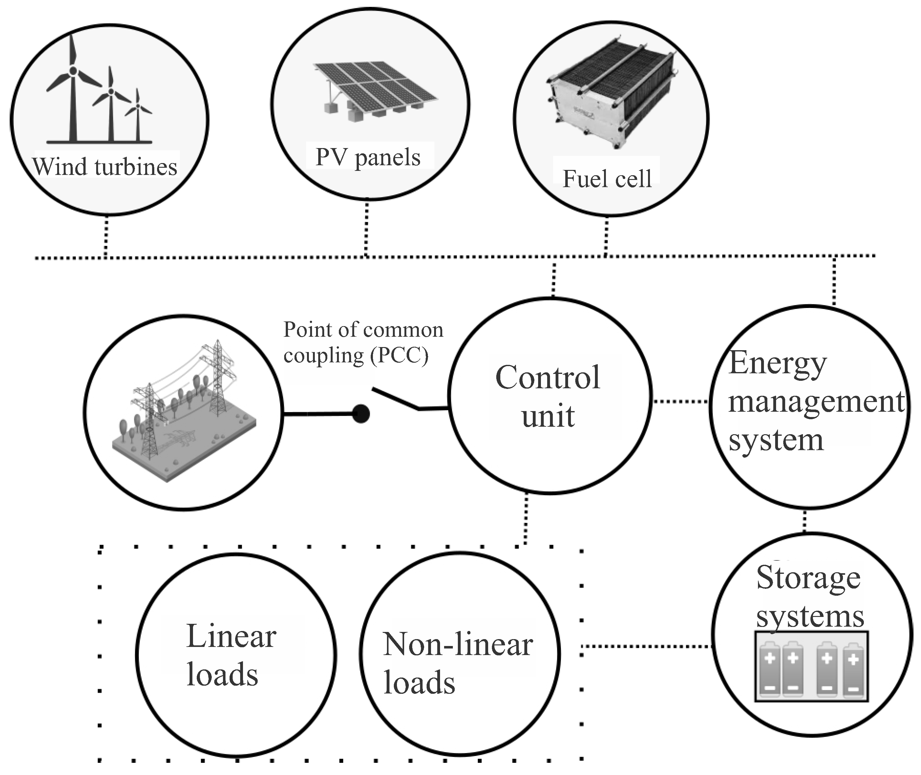
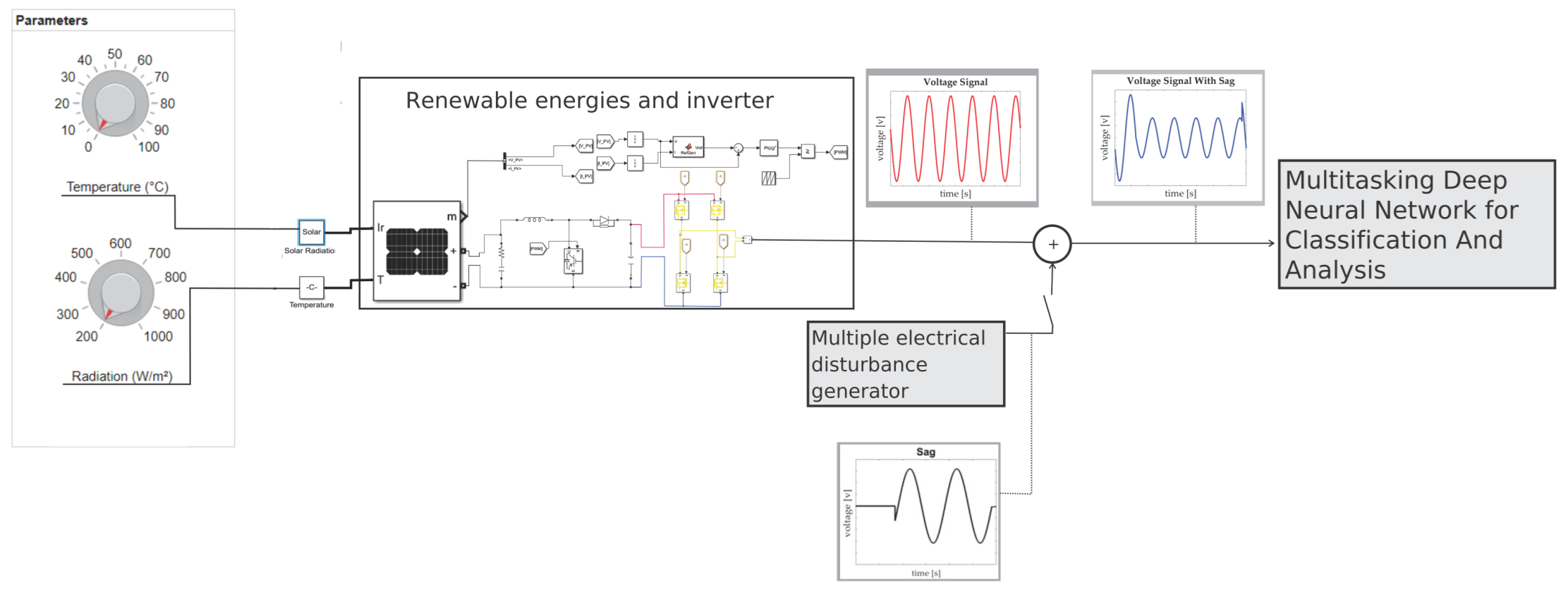
4.2. Description of Power System

The microgrid model used is an island-type grid with a photovoltaic system developed in the Matlab 2021b environment with the Simulink and AppDesigner tools and it introduces different electrical disturbances with different levels of complexity, as shown in the previous section. A photovoltaic system mainly integrates the configuration of the island-type microgrid model shown in Figure 1. A user can manipulate the variables of temperature and solar irradiation through an interface developed in App Designer. The architecture used in this contribution is shown in the Figure 5.

The components of the system include:

• Distributed generators: A solar photovoltaic system generates a maximum power of 250 kW in STC (cell temperature of 25 °C with solar irradiance of 1000 $\frac{\mathrm{W}}{{\mathrm{m}}^2}$).
• Voltage controller for distributed generators: DC-DC Boost type charge controller and a DC-AC voltage source inverter (VSI).
• Voltage inverter: For the Voltage Source Inverter (VSI), a full bridge inverter works at 1000 Hz switching.
• Control methodology for voltage controller: The system also has an integrated maximum power point tracking (MPPT) controller with a DC-DC boost type voltage controller. The MPPT control helps to generate the proper voltage by extracting the maximum power and adjusting the duty cycle to avoid performance problems due to changes in temperature and solar irradiance that are simulated in the system.

Although this microgrid model was used, it is important to mention that the methodology is designed to be implemented in various architectures. This is because only voltage signals are used to classify and analyze multiple electrical disturbances.

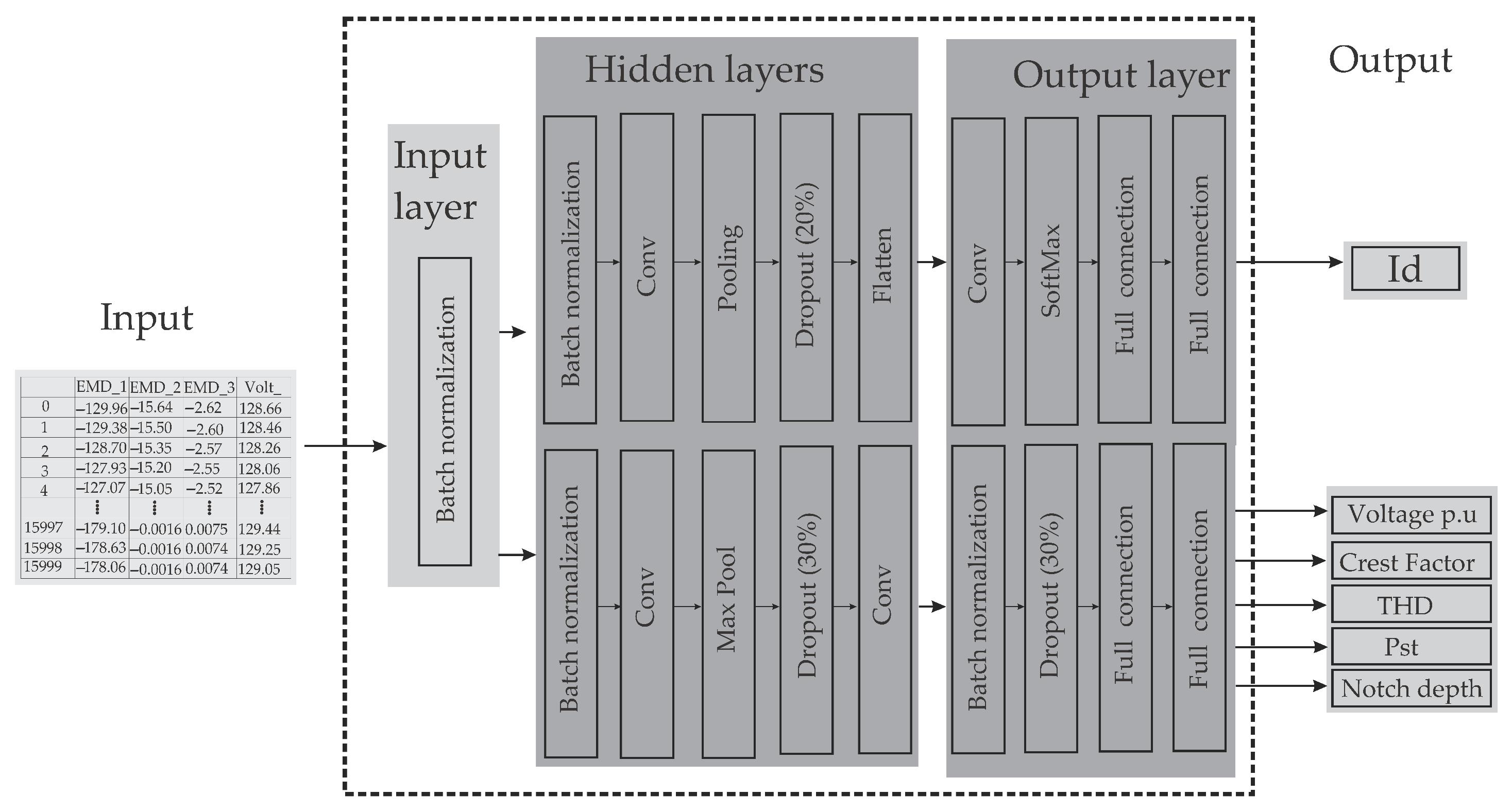
4.3. Deep Neural Network Multitasking Architecture

Figure 6 shows the architecture used for multitasking learning. The following points show the description of each layer and discuss different issues, such as how the layer works and its objective in the deep neural network, among other important points discussed. This allows us to observe more straightforwardly the function and composition of the neural network and how the information flows, how the data are processed, and how they are normalized to reduce computational consumption.

The components of this architecture are as follows:

• Batch Normalization: This layer is used to improve the training speed and stability of the model. The basic idea behind batch normalization is to normalize the input data of each layer [32]. This is accomplished by subtracting the batch mean from each input data point and dividing it by the batch standard deviation. The batch means and standard deviation are estimated using the input data of a batch rather than the entire data set [33]. Batch normalization helps to reduce the problem of internal covariate drift, which occurs when there is high variation in the input data. This can lead to slower convergence and overfitting [34]. Batch normalization is a powerful technique that improve the performance of deep neural networks [35].
• Convolutional layer or conv layer: This is a crucial building block of convolutional neural networks (CNNs). It is designed to perform feature extraction from input data such as images, video, or audio. The basic idea behind convolutional layers is to apply a set of learnable filters (kernels or weights) to the input data to extract essential features [36]. Each filter performs a convolution operation on the input data, which involves sliding the filter over the input and computing the dot product between the filter weights and the local input values at each position [37]. In a Convolutional Neural Network (CNN) used for regression, the convolutional layers will be designed to extract relevant features from the input data that help predict the target values. The convolutional layers are an essential part of the network architecture for regression problems because they allow the network to capture important local patterns in the input data, which can be highly relevant for predicting the target values. By stacking multiple convolutional layers with increasing filter sizes, the network can learn increasingly complex and abstract features from the input data, making more accurate predictions [38].
• Polling: This is used for down-sampling. The aim is to scale and map the data after feature extraction, reduce the dimension of the data, and extract the important information, thus performing feature reduction efficiently within the neural architecture. This avoids adding extra phases and and reduces computational consumption [39]. There are several types of pooling layers, but the most common ones are max pooling and average pooling. Max Pooling Layers reduce the spatial dimensions of the output from the convolutional layers by taking the maximum value within each pooling window [40].
• Dropout: This randomly drops out some of the neurons in the previous layer during training, which helps prevent overfitting and improves the network’s generalization ability. The main idea behind dropout is that the network learns to rely on the remaining neurons to make accurate predictions. This forces the network to learn more robust features that are not dependent on any specific set of neurons [41].
• SoftMax: This is a typical activation function used in neural networks, particularly in multi-class classification problems. The SoftMax function takes a vector of real-valued scores as input and normalizes them into a probability distribution over the classes [42].
• The flattening layer: This is a layer that converts multidimensional inputs into a one-dimensional vector. This is often performed to connect a convolutional layer to a fully connected layer, which requires one-dimensional inputs [43].
• Fully connected layer or dense layer: This is a layer where each neuron is connected to every neuron in the previous layer. Each neuron performs a weighted sum of the activations from the previous layer and then applies an activation function to the sum to produce an output. The weights and biases are learned during training using backpropagation, where the gradients are propagated backward from output layer to input layer [44].

5. Analysis and Results

Figure 7 shows the graphical display of feature extraction with the Empirical Mode Decomposition (EMD) algorithm. Various multiple or ultrafast disturbances with noise and without noise are shown. It is essential to do this so that the difference in complexity is noticed when developing a system trained with clean signals to work with signals with noise between 10 dB and 50 dB. Figure 7 shows an ultrafast frequency disturbance called Spike, which is difficult to detect with the human eye and often with sophisticated analysis and detection systems because the phenomenon lasts nanoseconds. The figure shows a spike without noise on the left side and a spike with noise on the right side.

The image is divided into three fringes; the first is the complete signal with the electrical disturbance, and the others are the Intrinsic Mode Functions (IMF) extracted as characteristics of the electrical disturbance. The Spike image shows how difficult it is to detect the disturbance; however, with IMF, it is easier to detect it, even when the signal has much noise. The Figure 8 presents the extraction of Notch features, which presents the same behavior as the previous image.

At a first glance, noticing where the electrical disturbance is located at which second is complex. However, extracting characteristics helps to detect where the ultra-fast disturbance occurs. In the same way with the Oscillatory transient, we can see how it shows the characteristics of the electrical disturbance that can be detected even with high noise levels in Figure 9.

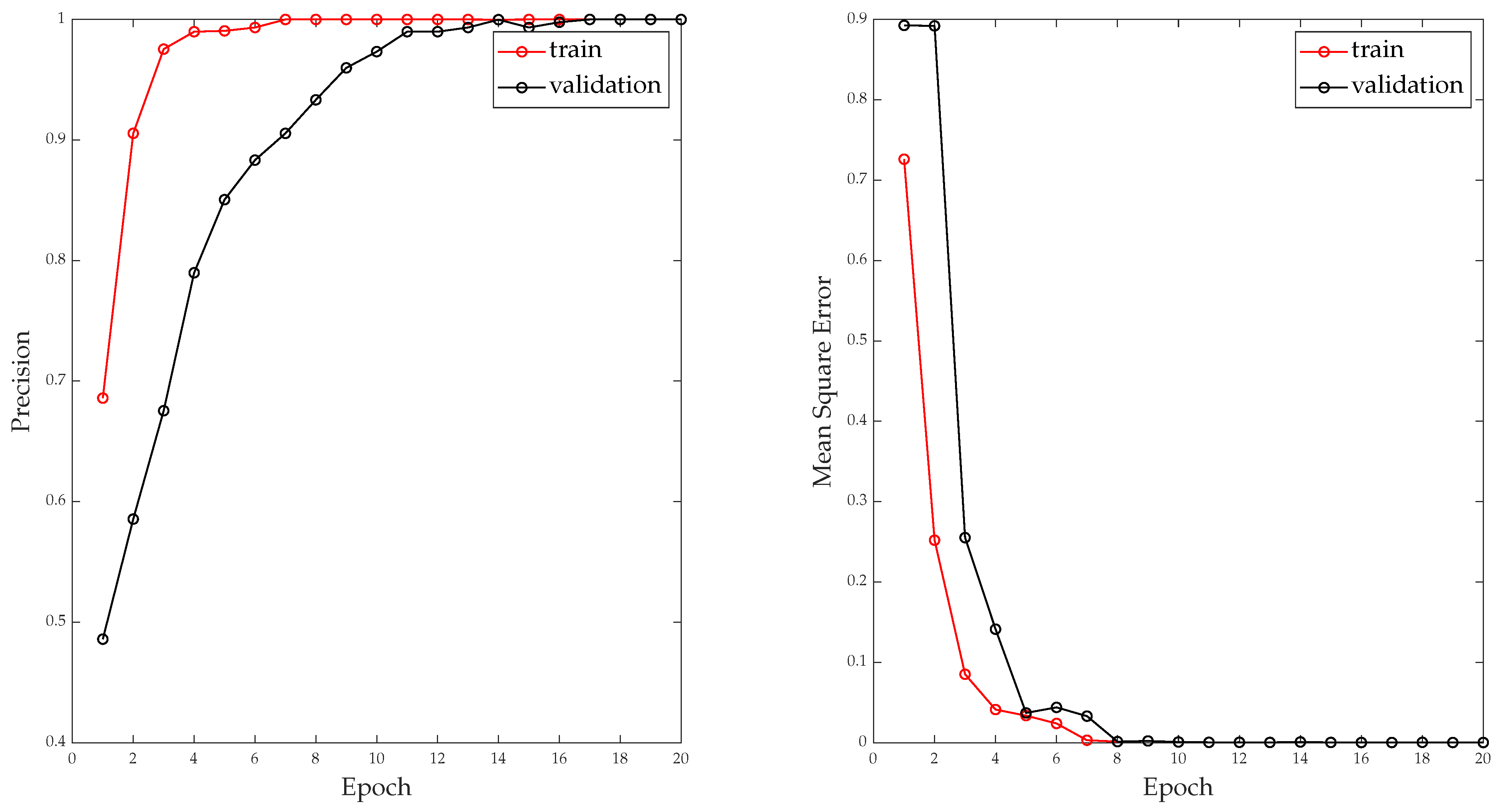
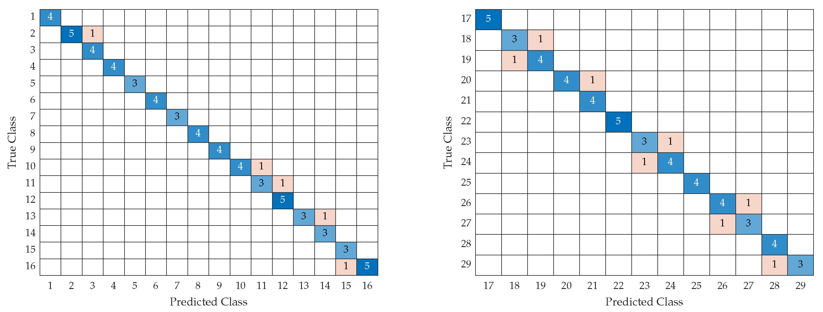
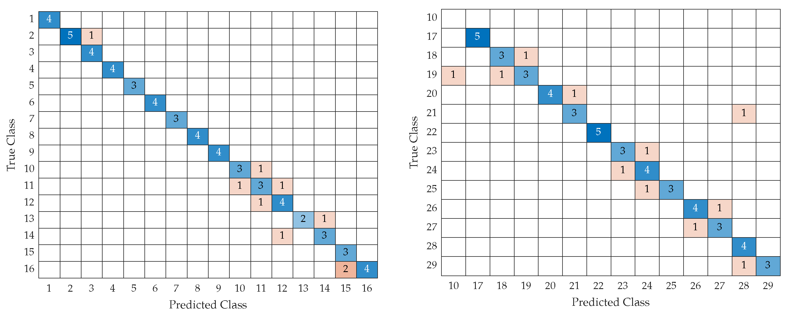
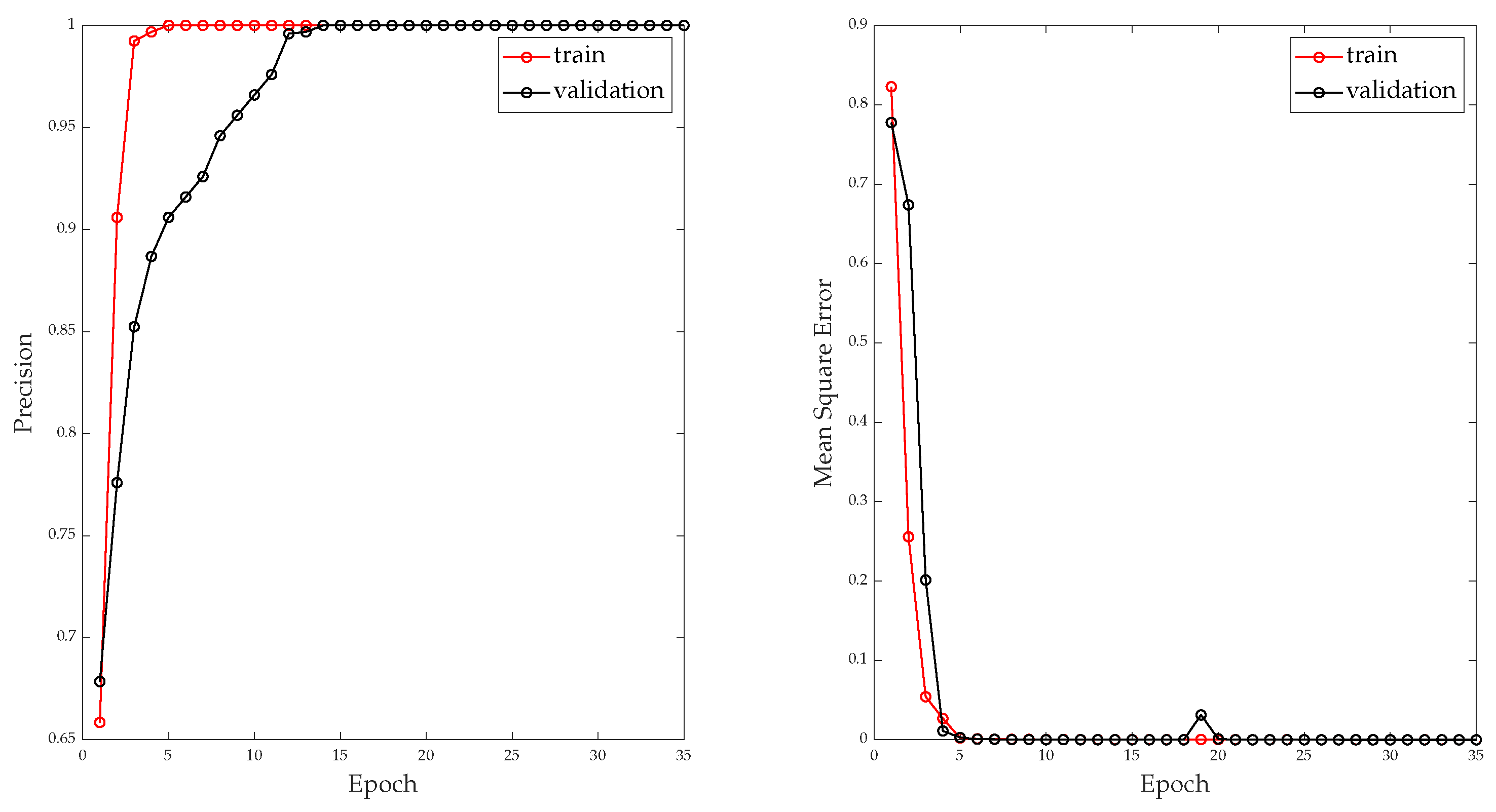
5.1. Signal Classification Performance Indices

The right side of Figure 10 shows the learning curve of the classification layer. This image graphically represents the behavior of the model in training and validation. It plots the value of the loss function (or error function) on the y-axis against the number of training iterations or epochs on the x-axis. The loss function measures the difference between the predicted outputs of the model and the actual outputs and is used to optimize the model during training.

Overall, the loss curve is an essential tool for understanding the performance of a machine learning algorithm during training and for diagnosing problems that may arise during the training process. On the other hand, the left side of Figure 10 shows the learning curve as a function of precision. It is possible to observe how it reaches an exact precision according to the graph and between values. However, performance is quantified beyond learning curves.

Tests were performed using the test data segment and graphically displayed in the following confusion matrix. The left side of Figure 11 shows the confusion matrix of the first 16 levels of electrical disturbances and the data set with about 750 electrical disturbances with different levels of complexity: clean disturbances and noisy disturbances between 10 dB and 50 dB. It can be observed how there are erroneous data, oscillating with an error between 5% and 2%. The right side of Figure 11 shows the second part, levels 17 to 29. It can be seen how a percentage ranging from 1.8% to 8.3% is obtained. Because this part’s complexity level increases, the model needs clarification to analyze the taxonomy of the last levels. This is because the last levels have much affinity between them due to the characteristics of the signals. The blue boxes correspond to the number of successes that the neural network had and the orange boxes are elements in which it had errors.

Additionally, tests were carried out on the power generation system described in Section 4.2. The left side of Figure 12 shows the transition matrix of the first part, that is, from levels 1 to 16 of electrical disturbances. One can notice how the percentage rises more, but this was because the number of disturbances was around 200 for the 29 levels. However, one can also notice how it retains a high accuracy value. The right side of Figure 12 shows part 2, with levels 17 to 29. Interestingly, the error level increases slightly in the last disturbances from levels 23 to 29. This is because levels 23 to 29 tend to have more affinity between them. However, an accuracy above 80% is maintained. The blue boxes correspond to the number of successes that the neural network had and the orange boxes are elements in which it had errors.

5.2. Performance Indices in Data Regression

For the regression task, the left side of Figure 13 shows the training curve in the context of error measurement. The right side of Figure 13 shows the training curve in the context of the accuracy of the regression task on the training and validation data segments.

The left side of Figure 14 shows the voltage analysis per unit of an electrical disturbance at 0.12 s. One can see how it detects a disturbance in the amplitude of more than 80%; that is, it is a severe disturbance. The right side of Figure 14 shows the same analysis, but with a noise of 40 dB; it shows how it is not affected and shows a voltage drop of 80%.

Figure 15 shows the analysis of the crest factor of a disturbance, remembering that the average value in the voltage signals is 1.4. The left side of Figure 15 shows how there are essential increases to consider. The right side of Figure 15 shows the analysis but in a disturbance with a noise of 40 dB. In this way, it is noted how the noise does not represent problems for the analysis and quantification model.

5.3. Analysis of Results

Table 6. Comparison of other investigations with the contributions of this paper.

	Reference	[17]	[45]	[14]	[22]	Current
Characteristics
Accuracy percentage		79.14–83.66%	90%	88–98%	91.3–99%	98–99%
Feature extraction methodology		short time Fourier Transform	Higher-Order Statistics	1-D convolutional	Wavelet Transform	Empirical Mode Decomposition (EMD)
Classification methodology		Convolutional Neural Networks Long Short-Term Memory	Multi-layer perceptron (MLP) Support Vector Machine (SVM)	Deep convolutional neural network	Support Vector Machine (SVM)	Multitasking Deep Neural Network
Electrical disturbance levels		7 levels	2 levels, Sags, and swells	15 levels	5 levels	28 levels
Noise levels		Without noise	40 dB to 60 dB	40 dB to 60 dB	Without noise	10 dB to 50 dB
Qualitative analysis of electrical disturbance		Does not perform quantification or analysis	Does not perform quantification or analysis	Does not perform quantification or analysis	Does not perform quantification or analysis	Quantitative analysis of the different electrical disturbances

compares critical elements for classifying methodologies for multiple electrical disturbances, such as the precision of the models, methodology to extract characteristics, classification methodology, levels of complexity of the electrical disturbances, the noise levels used, and finally, if any of these proposals offer any other methodology for the analysis and quantification of electrical disturbances.

With this comparative table, exciting points are inferred. First, the percentage of precision is not very variable among the classification proposals, and most remain above 90%. However, there is beginning to be a high concentration in some attributes, feature extraction, and classification methodologies based on deep learning or machine learning. Artificial intelligence is a discipline that has played a significant role in various contexts in the analysis and monitoring of electrical disturbances. The levels of electrical disturbances present how some are reduced to sags and swell, with 5 levels of disturbances or 15 levels. These contributions present a notable bias to classify disturbances that emerge from the amplitude. This is because working with frequency disturbances could often be complex and challenging if noise is added. This element compares with that in this proposal, although the range oscillates between 40 dB and 60 dB, whereas our proposal represents less noise than 10 dB or 20 dB. It is important to note that the level of complexity increases as the signal is noisier. Furthermore, one can note how none of these proposals work with quantifying and analyzing electrical disturbances. They only give a taxonomy with labels for the type of disturbance that occurs. It is essential to mention that measuring and analyzing the main quality and energy factors develops more direct and informative energy quality reports.

5.4. Discussions and Applications

Table 6 shows important characteristics for analyzing the performance of the deep neural model. An essential element in addition to precision, response time, and computational consumption is the ability of the classification methodology to detect events that interfere with electrical power quality remotely, that is, to identify events that could occur in distributed generators remote to the point central. The discrepancy of electrical disturbances is significant only to consider the disturbances that decrease the distribution system. We can see this in [11], where the discrimination of ultra-fast disturbances are carried out by feature extraction, a non-optimal element. This is because it does not have similarities with the characteristics of the signal components with the severity and the impact on the energy generating system. In the work of [46], the author shows a classification performance of over 90% with a noise range from 30 dB to 55 dB. However, the task of quantifying and detecting disturbances remotely are elements that are not considered for the development of this proposal. Within this type of contribution, it is very common to make complex proposals with a high consumption only to carry out simple classifications, as we can see in the work of [47]. Although this scientific contribution could be relevant, applying it in a tangible space in real time could be less practical due to computational consumption.

It is important to mention that this system focuses on classifying and quantifying electrical disturbances. When we refer to quantification, it is determining the level of impact on voltage and frequency and determining the main effects on the quality of electrical energy. Inferring the origin of electrical disturbances is an area of scientific and technological research within electrical micro grids. A system with a high level of intelligence is necessary where fuzzy logic, neural networks, and metaheuristic algorithms play an important role.

Within the applications are single-phase and three-phase systems for power quality analysis, analysis of multiple or single electrical disturbances, and optimization in detecting and treating problems. In this way, the studies in diverse electric generation and distribution systems of different powers could have more significant studies on the quality of energy, quantifying the impact of electrical disturbances and analyzing the quality of the wave distributed in the charging system. It is important to mention that this methodology benefits a large population sector; for example, there are regions where electricity is difficult to access. There are rural or remote communities where access to the main network may be limited or expensive. These communities benefit from having access to basic services such as lighting, refrigeration, communications, and energy for productive activities. On the other hand, various industrial or commercial areas ensure a continuous and reliable supply of energy and reduce greenhouse gas generation. This is especially important in critical sectors such as hospitals, data centers, hotels, shopping centers, and manufacturing industries, among others, where an interruption in the electrical supply can have serious economic or security consequences. In addition, within the research, they offer a testing and experimentation environment for developing and researching energy generation and storage technologies. Universities, research centers, and laboratories benefit from carrying out studies and tests in a controlled environment, which drives innovation and advancement in the energy field, as well as in public services, to improve the efficiency and reliability of the electrical system in general. Utility companies benefit by managing and optimizing power distribution, reducing losses, and adapting to growing power demand more efficiently. The generators distributed within electrical microgrids usually use renewable energy sources, such as solar, wind, or biomass, contributing to reducing greenhouse gas emissions and caring for the environment. These decentralized solutions promote clean energy generation and the transition towards a more sustainable energy model.

6. Conclusions

This article proposes a new multitasking deep neural network for classifying and analyzing multiple electrical disturbances. The Empirical Mode Decomposition (EMD) algorithm was used to extract the signal characteristics, specialized in non-stationary signals and non-linear intrinsic elements of electrical disturbances. The methodology’s performance was quantified using traditional performance indices for the regression and classification layers of the signal under different levels of complexity of noise and levels of complexity in disturbances. This methodology shows an accuracy of over 90% regardless of the noise level and the electrical disturbances’ complexity. The different tests showed how the methodology performs excellently, classifying and analyzing the ultra-fast frequency and amplitude disturbances. In addition to having noise in the signal, the percentage of precision remained above 90%. The EMD feature extraction algorithm was an excellent tool for processing the data and preserving the accuracy of the algorithm. It is essential to mention that, in addition to presenting a methodology for the classification and quantification of essential values for the quality of electrical energy and its study, with a high degree of precision and different levels of difficulty, the development of a methodology with various synthetic disturbances is presented, having as an advantage the ease of generating a diverse set of data and performing performance tests with different levels and diversity of electrical disturbances and with generators of different power. In this way, the proposed methodology is tested to face the scalability challenge of the different electricity generation systems.

References

1. Souza Junior, M.E.T.; Freitas, L.C.G. Power Electronics for Modern Sustainable Power Systems: Distributed Generation, Microgrids and Smart Grids—A Review. Sustainability 2022, 14, 3597. [Google Scholar] [CrossRef]
2. Prashant; Siddiqui, A.S.; Sarwar, M.; Althobaiti, A.; Ghoneim, S.S.M. Optimal Location and Sizing of Distributed Generators in Power System Network with Power Quality Enhancement Using Fuzzy Logic Controlled D-STATCOM. Sustainability 2022, 14, 3305. [Google Scholar] [CrossRef]
3. IEEE Std 1159-2019; IEEE Recommended Practice for Monitoring Electric Power Quality. IEEE Standards Association: New York, NY, USA, 2019.
4. Masetti, C. Revision of European Standard EN 50160 on power quality: Reasons and solutions. In Proceedings of the 14th International Conference on Harmonics and Quality of Power-ICHQP 2010, Bergamo, Italy, 26–29 September 2010; pp. 1–7. [Google Scholar] [CrossRef]
5. Ma, C.T.; Gu, Z.H. Design and Implementation of a GaN-Based Three-Phase Active Power Filter. Micromachines 2020, 11, 134. [Google Scholar] [CrossRef] [PubMed] [Green Version]
6. Ma, C.T.; Shi, Z.H. A Distributed Control Scheme Using SiC-Based Low Voltage Ride-Through Compensator for Wind Turbine Generators. Micromachines 2022, 13, 39. [Google Scholar] [CrossRef]
7. Wan, C.; Li, K.; Xu, L.; Xiong, C.; Wang, L.; Tang, H. Investigation of an Output Voltage Harmonic Suppression Strategy of a Power Quality Control Device for the High-End Manufacturing Industry. Micromachines 2022, 13, 1646. [Google Scholar] [CrossRef]
8. Yoldaş, Y.; Önen, A.; Muyeen, S.; Vasilakos, A.V.; Alan, I. Enhancing smart grid with microgrids: Challenges and opportunities. Renew. Sustain. Energy Rev. 2017, 72, 205–214. [Google Scholar] [CrossRef]
9. Jumani, T.A.; Mustafa, M.W.; Rasid, M.M.; Mirjat, N.H.; Leghari, Z.H.; Saeed, M.S. Optimal Voltage and Frequency Control of an Islanded Microgrid using Grasshopper Optimization Algorithm. Energies 2018, 11, 3191. [Google Scholar] [CrossRef] [Green Version]
10. Samanta, H.; Das, A.; Bose, I.; Jana, J.; Bhattacharjee, A.; Bhattacharya, K.D.; Sengupta, S.; Saha, H. Field-Validated Communication Systems for Smart Microgrid Energy Management in a Rural Microgrid Cluster. Energies 2021, 14, 6329. [Google Scholar] [CrossRef]
11. Banerjee, S.; Bhowmik, P.S. A machine learning approach based on decision tree algorithm for classification of transient events in microgrid. Electr. Eng. 2023, 1–11. [Google Scholar] [CrossRef]
12. Mahela, O.P.; Shaik, A.G.; Khan, B.; Mahla, R.; Alhelou, H.H. Recognition of Complex Power Quality Disturbances Using S-Transform Based Ruled Decision Tree. IEEE Access 2020, 8, 173530–173547. [Google Scholar] [CrossRef]
13. Liu, H.; Hussain, F.; Yue, S.; Yildirim, O.; Yawar, S.J. Classification of multiple power quality events via compressed deep learning. Int. Trans. Electr. Energy Syst. 2019, 29, 2010. [Google Scholar] [CrossRef]
14. Wang, S.; Chen, H. A novel deep learning method for the classification of power quality disturbances using deep convolutional neural network. Appl. Energy 2019, 235, 1126–1140. [Google Scholar] [CrossRef]
15. Thirumala, K.; Pal, S.; Jain, T.; Umarikar, A.C. A classification method for multiple power quality disturbances using EWT based adaptive filtering and multiclass SVM. Neurocomputing 2019, 334, 265–274. [Google Scholar] [CrossRef]
16. Shen, Y.; Abubakar, M.; Liu, H.; Hussain, F. Power Quality Disturbance Monitoring and Classification Based on Improved PCA and Convolution Neural Network for Wind-Grid Distribution Systems. Energies 2019, 12, 1280. [Google Scholar] [CrossRef] [Green Version]
17. Garcia, C.I.; Grasso, F.; Luchetta, A.; Piccirilli, M.C.; Paolucci, L.; Talluri, G. A Comparison of Power Quality Disturbance Detection and Classification Methods Using CNN, LSTM and CNN-LSTM. Appl. Sci. 2020, 10, 6755. [Google Scholar] [CrossRef]
18. Jasiński, M.; Sikorski, T.; Kostyła, P.; Leonowicz, Z.; Borkowski, K. Combined Cluster Analysis and Global Power Quality Indices for the Qualitative Assessment of the Time-Varying Condition of Power Quality in an Electrical Power Network with Distributed Generation. Energies 2020, 13, 2050. [Google Scholar] [CrossRef] [Green Version]
19. Subudhi, U.; Dash, S. Detection and classification of power quality disturbances using GWO ELM. J. Ind. Inf. Integr. 2021, 22, 100204. [Google Scholar] [CrossRef]
20. Radhakrishnan, P.; Ramaiyan, K.; Vinayagam, A.; Veerasamy, V. A stacking ensemble classification model for detection and classification of power quality disturbances in PV integrated power network. Measurement 2021, 175, 109025. [Google Scholar] [CrossRef]
21. Chamchuen, S.; Siritaratiwat, A.; Fuangfoo, P.; Suthisopapan, P.; Khunkitti, P. Adaptive Salp Swarm Algorithm as Optimal Feature Selection for Power Quality Disturbance Classification. Appl. Sci. 2021, 11, 5670. [Google Scholar] [CrossRef]
22. Saxena, A.; Alshamrani, A.M.; Alrasheedi, A.F.; Alnowibet, K.A.; Mohamed, A.W. A Hybrid Approach Based on Principal Component Analysis for Power Quality Event Classification Using Support Vector Machines. Mathematics 2022, 10, 2780. [Google Scholar] [CrossRef]
23. Cuculić, A.; Draščić, L.; Panić, I.; Ćelić, J. Classification of Electrical Power Disturbances on Hybrid-Electric Ferries Using Wavelet Transform and Neural Network. J. Mar. Sci. Eng. 2022, 10, 1190. [Google Scholar] [CrossRef]
24. Sun, J.; Chen, W.; Yao, J.; Tian, Z.; Gao, L. Research on the Roundness Approximation Search Algorithm of Si3N4 Ceramic Balls Based on Least Square and EMD Methods. Materials 2023, 16, 2351. [Google Scholar] [CrossRef] [PubMed]
25. Eltouny, K.; Gomaa, M.; Liang, X. Unsupervised Learning Methods for Data-Driven Vibration-Based Structural Health Monitoring: A Review. Sensors 2023, 23, 3290. [Google Scholar] [CrossRef]
26. Xu, D.; Shi, Y.; Tsang, I.W.; Ong, Y.S.; Gong, C.; Shen, X. Survey on Multi-Output Learning. IEEE Trans. Neural Netw. Learn. Syst. 2020, 31, 2409–2429. [Google Scholar] [CrossRef] [PubMed] [Green Version]
27. Tien, C.L.; Chiang, C.Y.; Sun, W.S. Design of a Miniaturized Wide-Angle Fisheye Lens Based on Deep Learning and Optimization Techniques. Micromachines 2022, 13, 1409. [Google Scholar] [CrossRef] [PubMed]
28. Liu, W.; Xu, D.; Tsang, I.W.; Zhang, W. Metric Learning for Multi-Output Tasks. IEEE Trans. Pattern Anal. Mach. Intell. 2019, 41, 408–422. [Google Scholar] [CrossRef]
29. Van Amsterdam, B.; Clarkson, M.J.; Stoyanov, D. Multi-Task Recurrent Neural Network for Surgical Gesture Recognition and Progress Prediction. In Proceedings of the 2020 IEEE International Conference on Robotics and Automation (ICRA), Paris, France, 31 May–31 August 2020; pp. 1380–1386. [Google Scholar] [CrossRef]
30. Yang, X.; Sun, H.; Sun, X.; Yan, M.; Guo, Z.; Fu, K. Position Detection and Direction Prediction for Arbitrary-Oriented Ships via Multitask Rotation Region Convolutional Neural Network. IEEE Access 2018, 6, 50839–50849. [Google Scholar] [CrossRef]
31. Igual, R.; Medrano, C.; Arcega, F.J.; Mantescu, G. Integral mathematical model of power quality disturbances. In Proceedings of the 2018 18th International Conference on Harmonics and Quality of Power (ICHQP), Ljubljana, Slovenia, 13–16 May 2018; pp. 1–6. [Google Scholar] [CrossRef]
32. Kaur, R.; GholamHosseini, H.; Sinha, R.; Lindén, M. Automatic lesion segmentation using atrous convolutional deep neural networks in dermoscopic skin cancer images. BMC Med. Imaging 2022, 22, 103. [Google Scholar] [CrossRef]
33. Zhao, R.; Wang, S.; Du, S.; Pan, J.; Ma, L.; Chen, S.; Liu, H.; Chen, Y. Prediction of Single-Event Effects in FDSOI Devices Based on Deep Learning. Micromachines 2023, 14, 502. [Google Scholar] [CrossRef]
34. Xu, S.; Zhou, Y.; Huang, Y.; Han, T. YOLOv4-Tiny-Based Coal Gangue Image Recognition and FPGA Implementation. Micromachines 2022, 13, 1983. [Google Scholar] [CrossRef] [PubMed]
35. Halbouni, A.; Gunawan, T.S.; Habaebi, M.H.; Halbouni, M.; Kartiwi, M.; Ahmad, R. CNN-LSTM: Hybrid Deep Neural Network for Network Intrusion Detection System. IEEE Access 2022, 10, 99837–99849. [Google Scholar] [CrossRef]
36. Naseer, S.; Saleem, Y.; Khalid, S.; Bashir, M.K.; Han, J.; Iqbal, M.M.; Han, K. Enhanced Network Anomaly Detection Based on Deep Neural Networks. IEEE Access 2018, 6, 48231–48246. [Google Scholar] [CrossRef]
37. Li, C.; Qiu, Z.; Cao, X.; Chen, Z.; Gao, H.; Hua, Z. Hybrid Dilated Convolution with Multi-Scale Residual Fusion Network for Hyperspectral Image Classification. Micromachines 2021, 12, 545. [Google Scholar] [CrossRef] [PubMed]
38. Sundaram, S.; Zeid, A. Artificial Intelligence-Based Smart Quality Inspection for Manufacturing. Micromachines 2023, 14, 570. [Google Scholar] [CrossRef]
39. Marey, A.; Marey, M.; Mostafa, H. Novel Deep-Learning Modulation Recognition Algorithm Using 2D Histograms over Wireless Communications Channels. Micromachines 2022, 13, 1533. [Google Scholar] [CrossRef]
40. Schmidhuber, J. Deep learning in neural networks: An overview. Neural Netw. 2015, 61, 85–117. [Google Scholar] [CrossRef] [Green Version]
41. Devaraj, J.; Ganesan, S.; Elavarasan, R.M.; Subramaniam, U. A Novel Deep Learning Based Model for Tropical Intensity Estimation and Post-Disaster Management of Hurricanes. Appl. Sci. 2021, 11, 4129. [Google Scholar] [CrossRef]
42. Nguyen, H.D.; Cai, R.; Zhao, H.; Kot, A.C.; Wen, B. Towards More Efficient Security Inspection via Deep Learning: A Task-Driven X-ray Image Cropping Scheme. Micromachines 2022, 13, 565. [Google Scholar] [CrossRef]
43. He, K.; Zhang, X.; Ren, S.; Sun, J. Deep Residual Learning for Image Recognition. In Proceedings of the 2016 IEEE Conference on Computer Vision and Pattern Recognition (CVPR), Las Vegas, NV, USA, 27–30 June 2016; pp. 770–778. [Google Scholar] [CrossRef] [Green Version]
44. Huang, S.; Wang, L. MOSFET Physics-Based Compact Model Mass-Produced: An Artificial Neural Network Approach. Micromachines 2023, 14, 386. [Google Scholar] [CrossRef]
45. Nagata, E.A.; Ferreira, D.D.; Bollen, M.H.; Barbosa, B.H.; Ribeiro, E.G.; Duque, C.A.; Ribeiro, P.F. Real-time voltage sag detection and classification for power quality diagnostics. Measurement 2020, 164, 108097. [Google Scholar] [CrossRef]
46. Sekar, K.; Kanagarathinam, K.; Subramanian, S.; Venugopal, E.; Udayakumar, C. An improved power quality disturbance detection using deep learning approach. Math. Probl. Eng. 2022, 2022, 7020979. [Google Scholar] [CrossRef]
47. Cao, H.; Zhang, D.; Yi, S. Real-Time Machine Learning-based fault Detection, Classification, and locating in large scale solar Energy-Based Systems: Digital twin simulation. Sol. Energy 2023, 251, 77–85. [Google Scholar] [CrossRef]
Figure 1. Smart microgrid architecture.
Technologies 11 00082 g001
Figure 2. Comparison of architectures between deep learning supervised learning and deep learning multitasking learning.
Technologies 11 00082 g002
Figure 3. Confusion Matrix Example.
Technologies 11 00082 g003
Figure 4. Methodology for the analysis and classification of multiple electrical disturbances.
Technologies 11 00082 g004
Figure 5. Photovoltaic power generator system for additional tests with a multiple electrical disturbance injector system.
Technologies 11 00082 g005
Figure 6. The architecture of a Novel Multitasking Deep Neural Network for Classification and Analysis of Multiple Electrical Disturbances.
Technologies 11 00082 g006
Figure 7. Feature extraction with EMD algorithm: (left) Spike without noise; (right) Spike with noise.
Technologies 11 00082 g007
Figure 8. Feature extraction with EMD algorithm: (left) Notch without noise; (right) Notch with noise.
Technologies 11 00082 g008
Figure 9. Feature extraction with EMD algorithm: (left) Oscillatory transient without noise; (right) Oscillatory transient with noise.
Technologies 11 00082 g009
Figure 10. Model training performance evaluation: (left) Precision of Multitasking Deep Neural Network—Classification; (right) Loss of Multitasking Deep Neural Network—Classification.
Technologies 11 00082 g010
Figure 11. Model training performance evaluation: (left) Test Data Segment Confusion Matrix—Part 2; (right) Test Data Segment Confusion Matrix—Part 2.
Technologies 11 00082 g011
Figure 12. Model training performance evaluation: (left) Test confusion matrix in photovoltaic power generating system—Part 1; (right) Test confusion matrix in photovoltaic power generating system—Part 2.
Technologies 11 00082 g012
Figure 13. Model training performance evaluation: (Left) Precision curve; (Right) Loss Learning curve.
Technologies 11 00082 g013
Figure 14. Analysis of voltage per unit in the electrical disturbance: (left) Voltage p.u in 0.12 s without dB disturbance or noise; (right) Voltage p.u in 0.12 s with Noise disturbance.
Technologies 11 00082 g014
Figure 15. Analysis of crest factor in the electrical disturbance: (left) No dB disturbance or noise; (right) Noise disturbance.
Technologies 11 00082 g015