Article

Forecasting by Combining Chaotic PSO and Automated LSSVR

1
Integration and Collaboration Laboratory, Department of Industrial Engineering and Engineering Management, National Tsing Hua University, Hsinchu 300, Taiwan
2
School of Mechatronical Engineering and Automation, Foshan University, Foshan 528000, China
*
Author to whom correspondence should be addressed.
Technologies 2023, 11(2), 50; https://doi.org/10.3390/technologies11020050
Submission received: 23 February 2023 / Revised: 24 March 2023 / Accepted: 27 March 2023 / Published: 30 March 2023
(This article belongs to the Special Issue 10th Anniversary of Technologies—Recent Advances and Perspectives)

Abstract

:
An automatic least square support vector regression (LSSVR) optimization method that uses mixed kernel chaotic particle swarm optimization (CPSO) to handle regression issues has been provided. The LSSVR model is composed of three components. The position of the particles (solution) in a chaotic sequence with good randomness and ergodicity of the initial characteristics is taken into consideration in the first section. The binary particle swarm optimization (PSO) used to choose potential input characteristic combinations makes up the second section. The final step involves using a chaotic search to narrow down the set of potential input characteristics before combining the PSO-optimized parameters to create CP-LSSVR. The CP-LSSVR is used to forecast the impressive datasets testing targets obtained from the UCI dataset for purposes of illustration and evaluation. The results suggest CP-LSSVR has a good predictive capability discussed in this paper and can build a projected model utilizing a limited number of characteristics.

1. Introduction

In addition to using the sample distributions that are provided, traditional statistical methods also base their estimation of the parameter’s value on the assumption that samples are infinite. The application of some outstanding statistics methods for the real-world issue is severely constrained. The major popular approach for nonlinear modeling, the artificial neural network (ANN), overcomes the limitations of conventional approaches for parameter estimation and may be built entirely from historical input-output data. The empirical risk minimization (ERM) principle-based ANN, however, there are several significant drawbacks, including the need for more training data, a lack of a consistent theoretical mathematical framework, the failure to find the fractional answers, overtraining, and dimension fatal event.
Support vector machine (SVM), a cutting-edge, potent machine learning technique created within the body of statistical learning theory (SLT), carries out the structural risk minimization (SRM) principle rather than the equivalent risk minimization (ERM) principle, giving it excellent generalization abilities in the case of small samples. SVM can effectively minimize modeling complexity, establish network structure automatically, and dimension disaster-free without local minima. Support vector regression (SVR) that had been proven its outstanding strength in many areas such as identification of patterns, regression analysis, forecasting in time-series, and optimization in numerous systems is expanded for resolving non-linear regression analysis.
A novel technique recently presented is termed the least squares SVR (LSSVR) [1], which uses equality constraints similar to that of a traditional artificial neural network (ANN). As the problem’s solution can be discovered using linearization, it is substantially simplified. It can be used to create a classification and prediction model, as seen in [2,3]. Yet, the right LSSVR meta parameter configuration determines how well LSSVR models perform. As a result, only “professional” users with a solid understanding of the SVR approach can handle the LSSVR program.
The proper three LSSVR settings determine the quality of LSSVR models. Secondly, in big-size cases, the LSSVR function is quite slow since a quadratic programming (QP) issue needs to be solved. Second, several crucial parameters that endure and impair LSSVR’s recapitulation capabilities, are not optimal in the LSSVR modeling. Finally, a predictive LSSVR model also has a hard time choosing some crucial properties. Furthermore, when the model interpretability is crucial, the issue could become more difficult to solve. How to choose these variables to guarantee outstanding recapitulation expression is a fundamental challenge in utilizing LSSVR for nonlinear systems. Evolutionary algorithms (EAs), particularly genetic algorithms (GAs), are the most popular method for determining parameters and characteristics, and they have already been used to choose characteristics and optimize parameters for the LSSVR model [4,5]. While particle swarm optimization (PSO), which is inspired by the swarm action from creatures, is extremely simple for installation as well as has fewer parameters for the tune, GA is challenging and is short of computational power. The simulation findings demonstrate that GA and PSO readily trap into local optimal solution, despite the fact that PSO can effectively employ in handling optimal problems of more dimensional [6,7,8,9,10,11].
Thus, this study must address the following three problems:
  • Initialization of the parameters: This is due to the possibility that it is unaware of the location of the global minimum at which the prior optimization problem was resolved.
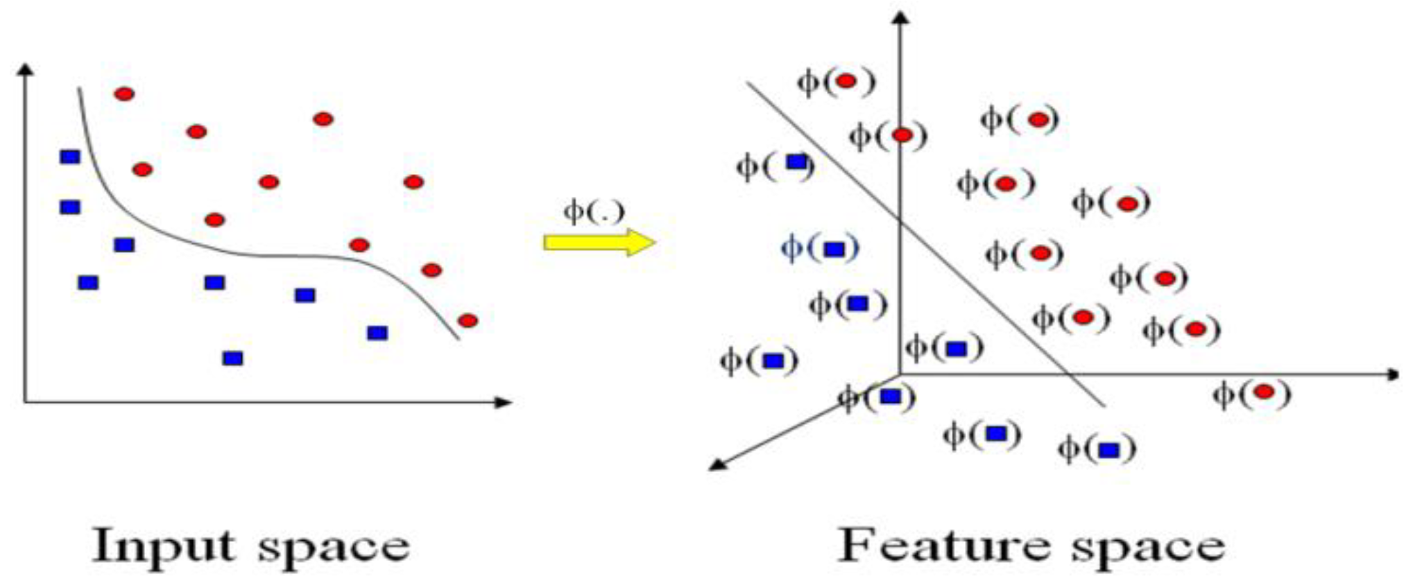
  • Characteristic extract or the characteristic evolution component can typically accomplish the decrease in data dimensionality. Often, this has been accomplished using characteristic extract methods like principal component analysis (PCA). The PCA is ineffective for this study’s objectives since it also wants to produce highly precise predictive models, not just reduce the dimensionality of the data. Nevertheless, the PCA doesn’t take into account the link for variables of input and variables of reply throughout the data reduction process, making it challenging to create a model that is extremely precise. Furthermore, if the input variables’ dimensionality is really high, it might be challenging to interpret the main components that are produced by the PCA. On the other hand, for data sets with high dimensionality, the PSO has been shown to perform better than other methods [11]. A simplified LSSVR model with improved generalization can be created by selecting more information for any data set provided when employing the fewest characteristics possible throughout the characteristic evolution phase.
  • Another PSO is employed in the parameter evolution component to optimize the LSSVR’s parameters. Generally, LSSVR generalization ability is governed by the type of kernel, parameters’ kernel, and parameter’s upper bound. Every form of the kernel has benefits and drawbacks, hence a mixed kernel makes sense [12,13,14]. Additionally, computational time and complexity in the training of the algorithm equals the total execution generations multiplied by the number of total solutions and multiplied by the time complexity of the update for each solution.
In this study, the chaotic particle swarm optimization (CPSO) approach has been used to tackle optimization issues. This novel PSO is based on chaos investigating, the logical model, and the tent model [15,16]. The advantage and innovation of the new regression method CP-LSSVR presented in this work is demonstrated as follows:
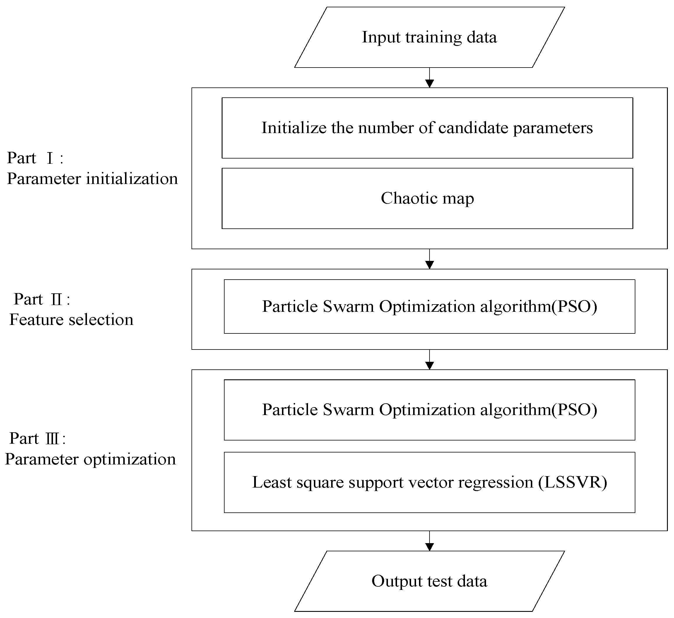
  • The CP-LSSVR is used to initialize the parameters for the parameters initialization issue of LSSVR applications.
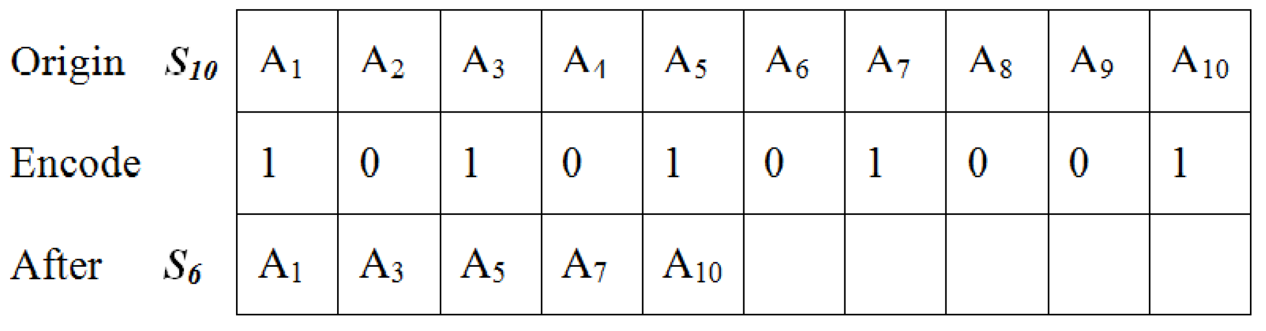
  • A binary PSO is utilized for feature selection in the input data to improve the model’s interpretability for the issue of requiring LSSVR to preprocess the input characteristics if the dimensions of input space or input characteristics are quite vast.
  • A third PSO is applied to optimize its parameters to boost the LSSVR’s capacity for normalization.
SVR, LSSVR, kernel function, Particle Swarm Optimization (PSO) algorithm, and chaotic sequences are all described in Section 2. In Section 3, the CP-LSSVR learning paradigm is thoroughly explained. Benchmark datasets, comparative methods, and the reported experimental results are described in Section 4. Conclusion and additional research have been analyzed in Section 5.

2. SVR and LSSVR

By applying a nonlinear function (m > d) to transfer an input of d-dimensionality onto an m-dimensional characteristic space, SVM regression (SVR) creates a linear model in the characteristic space. The process is depicted in Figure 1.
Let’s assume a training data set { x k , y k } k = 1 N , where x k n as well as y k for k = 1, …, N and represent characteristics’ input space and objective value, respectively. N denotes the training data’s size. In order to translate the input data to an advanced dimensional characteristic space, the SVR must identify a nonlinear map from input space to output space. Then, Equation (1) shows the linear regression using the following estimate function [17]:
l ( x ) = a ϕ ( x )   + e
where a is the coefficients, ϕ ( x )   signifies a sequence of nonlinear transformations that translates the input space into the characteristic space, and e means a real number. To reduce the risk is the goal is shown in Equation (2) [1]:
min a , e , E k u , E k l                 F ( a , e , E k u E k l ) = | | a | | 2 2 + C k = 1 N ( E k u + E k l )       s . t                           y k ( a ϕ ( x k ) ) + e σ + E k l                                         ( a ϕ ( x k ) ) + e y k σ + E k u                                         E k u , E k l 0                           k = 1 , , N
The characteristic map ϕ   vector has transferred the dataset of k-sample’s vector to a advanced-dimensional space, and     E k u is training error of upper bound and     E k l presents training error of lower bound for the σ-insensitive tube.
| y ( a ϕ ( x ) + e ) | σ
The dual formulations solution may be sparse due to the σ-insensitive loss model that also precludes the complete training set from fulfilling the boundary requirements. A balance achieved between the flatness of F and its accurateness in catching the training data is determined by the item | | a | | 2 2 , which is known as the normalization item, and C, which presents the normalization constant.
Equation (3) suggests that the tube σ contains the majority of the data αk. An error     E k l or     E k l has been typically tried to reduce in the objective function if αk is outside the tube. This is depicted in Figure 2. By minimizing the normalization term | | a | | 2 2 as well as the training error C k = 1 N ( E k u + E k l ) , SVR prevents the training data to be underfitted and overfitted.
The Karush-Kuhn-Tucker methods [18] require introduction of Lagrange multipliers γ k , γ k * , and the SVR approach aggregates to solving the convex quadratic model given in Equation (4)
min γ , γ *               1 2 k , s = 1 N ( γ k γ k * ) ( γ s γ s * ) K ( x k , x s ) + σ k = 1 N ( γ k + γ k * ) k = 1 N y ( γ k γ k * ) s . t                 k = 1 N ( γ k γ k * ) = 0                             0 γ k , γ k * C
SVMs are superior to other regression techniques because they solve the quadratic programming (QP) problem without hitting the local minima that depend on the statistical learning theory and the structural risk minimization concept [18]. The non-linear SVR function in this work is LSSVR. LSSVR employed was selected as the estimation approach due to its superior normalization power and ability to produce an almost global answer in a reasonable amount of training time [19]. The optimization problem’s basic formulation of an LSSVR regression model in characteristic space is Equation (5) [19]:
min a , e , π                 F ( a , e , π ) = | | a | | 2 2 + C k = 1 N π k 2 2 s . t                   y k ( a T · ϕ ( x k ) + e ) = π k                       k = 1 , 2 , N
Due to the weighting vector’s extremely high dimension, the calculation of Equation (5) is very challenging. This issue can be resolved by computing the model through a Lagrangian stated in Equation (6) in a dual space as opposed to the primal space.
L ( a , e , π , γ ) = F ( a , e , π ) C k = 1 N γ k { a T · ϕ ( x k ) + e + π k y k }
where γ k is the support vector that belongs to the real number, often known as the Lagrange multiplier. In light of this, Equation (7) lists the prerequisites for optimality.
L a = 0 a = k = 1 N γ k ϕ ( x k ) L e = 0 k = 1 N γ k = 0 L π k = 0 γ k = C π k L γ k = 0 a T ϕ ( x k ) + e + π k y k = 0 k = 1 ,   ,   N
After removing π and a, the answer is obtained as Equation (8).
[ 0             1 T 1           Ω + τ 1 I ] [ e γ ] = [ 0 y ]
where y = ( y 1 , , y n ) T ,   I = ( 1 , 1 ) T ,   γ = ( γ 1 , , γ n ) T ,   Ω k s = ( ϕ ( x k ) ) T ϕ ( x s ) for k,s = 1, …, N. There is a mapping and an expression that may be written as k ( x , y ) = k ϕ k ( x ) T ϕ k ( y ) based on Mercer’s condition. Hence, the kernel k ( . , . ) is constructed such that Equation (9).
k ( x k , x s ) = ϕ ( x k ) T ϕ ( x s )
where ϕ represents the formula that simulates the real non-linear mapping formula and x k as well as x s denoted as both goals for the data set.
In Equation (10), the outcome LS-SVR model for function estimation is found.
l ( x ) = k = 1 N γ k · υ ( x k , x s ) + e
where x k and e are the answers to Equation (10).
Complex non-linear data can be mapped using kernels into an advanced-dimensional characteristic space that linear modeling is feasible. Due to the difficulty in determining the mapping model and the overall lack of prior knowledge, the characteristic space is completely created by calling a common kernel model. A kernel model (K) works on two input vectors as shown in Equation (9).
To build a linear function in the characteristic space, one does not need to be aware of the actual underlying feature map when using a kernel function. In literature, a number of kernel functions are frequently utilized.
The width of the tube, the mapping function, and the error cost C are the three parameters in this study that define the LSSVR quality. The nonlinear mapping is performed by the Mercer kernel’s approximate characteristic map. Equations (11)–(13) show the common kernel functions in machine learning theories [20].
Linear kernel:
κ ( x k , x s ) = x k T · x s
Kernel of a polynomial:
κ ( x k , x s ) = ( x k T · x s + h ) g
Gaussian (RBF) kernel:
κ ( x k , x s ) = exp ( x k x s 2 2 σ 2 )
The parameters xk and xs are vectors in the input space; g signifies the polynomial’s level and T presents the item of intercept constant in Equation (12) and σ2 indicates the Gaussian kernel’s width in Equation (13).
The polynomial kernel (a global kernel), among the three standard kernels, stated earlier, exhibits stronger extrapolation capabilities at lower orders of levels but needs higher orders of levels for effective inserted values. The RBF kernel, a local kernel, excels in inserted values but falls short in extrapolating across longer distances.
It is difficult to declare which kernel is the greatest across the board, though, because each has pros and cons. According to the studies [13,21], combining or hybridizing various kernel functions can enhance SVM’s generalization capabilities. In this paper, the LSSVR model using a mixed kernel is trained. The three kernels mentioned above are combined to form the mixed kernel. It is possible to write the convex combination kernel by Equation (14).
κ = λ 1 κ l i n e a r + λ 2 κ p o l y + λ 3 κ r b f w h e r e λ 1 + λ 2 + λ 3 = 1 , 0 λ 1 , λ 2 , λ 3 1
Since all kernel functions in the proposed mixed kernel fulfill Mercer’s theory, a convex combination of them fulfills the theory, too.

3. LSSVR Based on Chaotic Particle Swarm Optimization (CPSO) Algorithm

The suggested automatic LSSVR learning paradigm is further detailed in this section. The automatic LSSVR learning paradigm is first introduced in its common structure. Then, every step of the chaotic map and PSO-based LSSVR parameter initialization, characteristic selection, and parameter optimization is discussed.

3.1. Automatic LSSVR Learning Paradigm

Several practical studies have shown that the LSSVM is a successful learning technique for regression issues [21,22,23]. For LSSVR applications, there are still three key issues.
  • Parameters initialization.
  • It is required for LSSVR to preprocess the input characteristics if the dimensions of input space or input characteristics are quite vast, in order to improve the interpretability of the LSSVR-based forecasting model.
  • This work adopts a mixed kernel model to get beyond the effect of kernel types because LSSVR normalization ability is frequently governed via (a) kernel type. The next two things, however, heavily rely on the researchers’ artistic ability. (b) kernel parameters: convex combination coefficients (λ1, λ2, λ3), and kernel parameters (g, σ). C is the upper bound parameter.
Software algorithms are employed to solve these three issues. A chaotic map is used to initialize the parameters for the first issue. In order to improve the model’s interpretability for the second issue, a binary PSO is utilized for feature selection in the input data. To boost the LSSVR’s capacity for normalization, a third PSO is applied to optimize its parameters. The automatic LSSVR learning paradigm, shown in Figure 3, is developed based on the three techniques.
It is simple to see that the automatic LSSVR learning paradigm has three basic components that address the aforementioned three major issues.
Use the chaotic map in the first section to defeat the PSO algorithm’s initialization’s randomly produced solutions.
The binary PSO searches a subset of characteristic variable subsets in the exponential space in the second section before sending that subset of characteristics to an LSSVR model. From each subgroup, the LSSVR extracts forecasting data and gains knowledge of the schemes. A trained LSSVR is tested on a holdout data set that was not utilized for training after learning the schemes in the data, and it then sends the calculation rule as a fitness function for PSO. The PSO biases its search direction according to fitness values to maximize the assessment aim. It is important to note that LSSVM just adopts the chosen characteristic variables during the training and evaluation processes.
The six unknown parameters (λ1, λ2, λ3, g, σ, C) are optimized in the third section using PSO. Section 3.2, Section 3.3 and Section 3.4 define in full the contents of each section.
To combine the two elements of evolution is feasible. It is possible to simultaneously optimize the characteristic evolution and the parameter evolution. It means the parameter optimization technique can be carried out prior to the characteristic selection procedure in the autonomous LSSVR learning paradigm. Large input characteristic dimensions are not recommended in reality due to the excessive computational workload. In this regard, it makes it more logical to undertake characteristic selection before parameter evolution.

3.2. Chaotic Sequences-Based Parameters Initialization

It might not know the position of the global minimum before an optimization problem is solved [13]. The PSO-generated solutions, however, use a random mechanism in the beginning stages, making it simple to reach the local optimal. This paper makes an effort to use chaotic sequences to tackle this issue.
  • Step 0. Generated by Logistic map chaotic sequence by Equation (15), following:
L ( k + 1 ) = n · L ( k ) · ( 1 L ( k ) ) , L ( k ) [ 0 , 1 ] ;   n [ 3.56 , 4 ]
  • Step 1. For the m particles in the D-dimensional space, the first generates a random initial value m:
L 1 ( 1 ) , L 2 ( 1 ) , , L m ( 1 )
  • Step 2. Chaotic sequence to the initial value of m-Equation (15). At that point, m will be the trajectory after Z iterations.
  • Step 3. Substituting the chaotic trajectory of the article from m in the selected Z iteration value into the Equation (16). One can compute x υ , k
x υ , k = L υ ( k ) ( max k min k ) υ / m + min k , υ = 1 , 2 , , m ; k = 1 , 2 , , Z
where x υ , k denotes the position of the υ particles in the k-dimensional space. L υ ( k ) is for the first υ particles in the randomly generated initial value of Equation (15) after k multiplying the value by the number of iterations.
Using Equation (16) calculated for all x υ , k components m row column Z Matrix as following Equation (17):
[ x 1 , 1 x 1 , 2 x 1 , Z x 2 , 1 x 2 , 2 x 2 , Z             x m , 1 x m , 2 x m , Z ]
where each row vector represents the initial position of a particle.

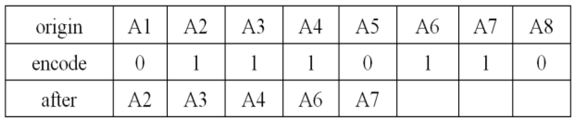
3.3. PSO-Based Input Features Evolution

The level of potential input variables might be rather big for many practical issues. It’s possible that some of these input variables are redundant. A significant input variables’ level will also raise LSSVR’s size, necessitating more training data and longer training periods to achieve a respectable level of normalization [22,23]. As a result, characteristic selection should be used to reduce input characteristics. Typically, the procedure of selecting a subset of the original characteristics by eliminating any duplicate or poorly-informed characteristics is referred to as characteristic selection [24].
The second challenge in the addressed automatic LSSVR learning paradigm is to choose crucial features for LSSVR learning. Two things are the major goals of characteristic selection:
  • To eliminate some less-important characteristics for decreasing the input characteristics’ size and enhance forecasting capability.
  • Additionally, it is to pinpoint several crucial characteristics that influence model performance, hence bringing down model complexity.
PSO, the most prevalent kind of software algorithm to date, has developed into a significant stochastic optimization technique, in contrast to most conventional optimization algorithms, because it frequently finds the optimal optimum. In this study, the input characteristic subset for LSSVR modeling is extracted using PSO.
The required particle number is initially set using the principles of particle swarm optimization, and the starting coding alphabetic string for every particle has been then generated at random. In this work, every particle is coded to mimic a chromosome using a common method; every particle is converted to a binary alphabetic string S = A 1 , A 2 , , A m , m = 1, 2, …, N, where bit value {1} presents a characteristic that has been chosen and bit value {0} denotes a characteristic that has not been chosen.
When utilizing particle swarm optimization to examine a 10-dimensional data set (m = 10), for instance, any characteristics’ level can be chosen fewer than m, i.e., it can randomly select six characteristics, as shown in the accompanying Figure 4.
The six characteristics in each data set serve as a representation of the data dimension and have been assessed via LSSVR while calculating the fitness score. Adaptive value serves as a foundation for every particle renewal. The best adaptive value within a group of p-best is g-best, while the best fitness value for every particle renewal is p-best. After obtaining p-best and g-best, it may monitor the characteristics of p-best and g-best particles in terms of their location and speed. The binary version of PSO is utilized in this investigation [25]. Each particle’s location is specified as a binary string that corresponds to a characteristic selection scenario [26].
The fitness function is the last evaluation criterion and is used to assess each string’s quality. The following Equation (18) can be used to build the fitness function for the PSO variable selection.
F i = 1 f i + m i c
where “ m i c ” is a decimal that is used to avoid the denominator being zero, f i representing the ith solution’s objective.
In this case, the relevancy of the input variables and the response variable is modeled using the LSSVR, as you may have noticed. The LSSVR models are then trained using training data, tested using holdout data, and the suggested model is assessed using the reduction LSSVR-error quadratic sum of the solution.
The aforementioned formulae determine how often each particle is updated. The PSO procedure’s pseudo code is shown below Algorithm 1.
Algorithm 1: PSO—Based Input Features Evolution
Goal: Reducing (1-hit ratio)
Input: training data set.
Output: The PSO-LSSVR’s characteristics set.
BEGIN
Establish the population
While (number of generations, or the halting requirement is not fulfilled)
For i = 1 (particles’ number)
When one’s fitness level Xk exceeds another’s p-best,
next update p-bestk = Xk
For υ belongs to neighborhood of Xk
  If fitness Xυ is higher than fitness of g-best,
Next update g-best = Xυ
  then υ
Every dimension g
V k , g ( h + 1 ) = a V k , g ( h ) + τ 1 c 1 ( P k , g x k , g ( h ) ) + τ 2 c 2 ( P j , g x k , g ( h ) )
S ( V k , g ( h + 1 ) ) = 1 1 + π V k , g ( h + 1 )
when  rand() < S ( V k , g ( h + 1 ) )
then X k , g ( h + 1 ) = 1
else   X k , g ( h + 1 ) = 0
  Next g
Next k
Next generation till the ending criteria
END
The function in Equation (19) determines the characteristic following renewal.
S ( V k , g ( h + 1 ) ) = 1 1 + π V k , g ( h + 1 )
If S ( V k , g ( h + 1 ) ) is greater than a disorder number generated at random and falling within the range of (0, 1), then its position value Am (m = 1, 2,…, N) denotes this characteristic has been chosen as a claimed characteristic for the next renewal as {1} otherwise, denotes this characteristic has not been chosen as a claimed characteristic for the next renewal as {0}.

3.4. PSO-Based Parameters Optimization

The current GA algorithm has some speed and accuracy restrictions for the convergence of high-dimensional problems, in addition to being complex in terms of selection, crossover, and mutation. The PSO algorithm, in contrast, is a parallel global search based on population strategy, the idea of which is straightforward and simple to implement. It also has a faster convergence speed, is able to handle high-dimensional problems while still having some advantages, and is a population-based stochastic optimization technique.
Theoretical benefits of the PSO algorithm, which was used in this study to perform a solution search for the six parameters of LSSVR.
Up until the termination condition is met, the process is repeated. The undetermined parameter, containing controlled parameters and Lagrange multipliers, constitutes the objects of evolution after the up-construction of the LSSVR model with adjustment [13,19,21]. This is due to the selection of these parameters significantly based on the theories of researchers. The parameters in this study are set up in common and appropriate ranges ( g : [ 0 , 6 ] ,   σ 2 : ( 0 , 1 ] and C : ( 0 , 20 ] ) to reduce computing costs.
As a result, a vector is described as a common notation of the parameters employed in the PSO-LSSVR training procedure as shown in Equation (20):
Ψ = ( λ 1 , λ 2 , λ 3 , g , σ , C , γ k , e )
It can now reformulate using the forecasting parameter constraints and the following model Equation (21).
min                     F ( Ψ ) = | | a | | 2 2 + C k = 1 N π k 2 2 s . t                         y k ( a T · ϕ ( x k ) + e ) = π k                   k = 1 , N                                   λ 1 + λ 2 + λ 3 = 1                                   λ 1 , λ 2 , λ 3 0                                   1 n # a t t r i b u t i o n s , n N +                                   0 g 6 ,       0 σ 1 ,       0 C 20
The automatic LSSVR learning paradigm with a mixed kernel, the best input characteristics, and the optimized parameters are created by the aforementioned evolutionary processes. Six outstanding datasets from the UCI dataset can be used as testing targets in Section 4 for the developed automatic LSSVR learning paradigm as an example and evaluation tool.

4. Experiment Findings

The benchmark datasets and similar approaches are initially introduced in this section. Then, it shows how to identify the essential features that influence the outcomes of the prediction and describe the optimization procedure. Lastly, it evaluates the effectiveness of the suggested automatic LSSVR in comparison to a few other predicting models.

4.1. Benchmark Datasets and Compared Approaches

It tested six datasets referred to the UCI Machine Learning Repository [27] to confirm the robustness of our method, as shown in Table 1 and in more detail in Table 2.
Individual CP-LSSVR models with polynomial, RBF, and tangent kernels, collectively referred to as CP-LSSVRlinear, CP-LSSVRpoly, and CP-LSSVRRBF, were trained using the PSO algorithm (PSO-LSSVR) for further comparison. The data used for training and testing was for the six datasets is listed in Table 1. For example, among the total observations of Boston Housing Data is 506, 304 data are used for training data and the remaining 202 data are used for testing data.

4.2. Characteristic Selection Using PSO

This study conducted six benchmarks to approve the PSO-based characteristic selection algorithm’s resilience.
To create a characteristic selection to avoid overlapping, the training data is randomly picked. As the training data’s size may be smaller than the test data or it might be too small to be regarded as typical training data, it reasoned that CP-LSSVR training with less than 50% training data is insufficient.
Three steps were included in each experiment.
  • Step 1: Use the initial value that the chaotic map process created in step 1 (for instance, the dataset Auto-Mpg Figure 5).
  • Step 2: Assess the fitness function.
  • Step 3: Before MCN.set w = 0.9 0.5 · j / M   C N ,   j = iteration , choose the number of input characteristics using Binary PSO.
  • Step 4: Selected training data k % (k = 50, 60,…, 100) are used to train the LSSVR with PSO.
  • Step 5: The trained LSSVR was tested for a set size.
Also, an AMD Turion (tm) 642 Mobile Technology TL-64 computer running at 2.2 GHz with 3 GB of memory was used to construct the PSO algorithm in the C++ programming language. The ideal values for these parameters are established in Table 3 following a test approach.
Table 4, Table 5, Table 6, Table 7, Table 8 and Table 9 display the chosen characteristics. It should be noted that the major characteristics chosen indicate the best characteristic sets for all tests and were chosen through six separate experiments using various data sets created via data partition approach.

4.3. PSO-Based Parameter Optimization for CP-LSSVR

The mixed kernel’s use in this paper also results in more unknown parameters. As a result, the chaotic initialization strategies are used, and the uncertain parameters comprise one feature election number, six controlled parameters, and N Lagrange multipliers.
Before providing the experimental findings, the evaluation criteria are specified for assessing the effects of the suggested algorithms. Present m is the quantity of the testing samples, y ^ i denotes the forecast value of y ^ , and y ¯ = i y i / m is the mean of y 1 , , y m without losing generality. Then, for algorithm evaluation, the following criteria are employed.
SSE: Sum squared error of testing, S S E = i = 1 m ( y i y ^ i ) 2 . SSE stands for fitting accuracy; the lower the SSE, the more accurately the estimate fits the data. If noises have been employed as testing samples, a low SSE likely indicates that the regressor is overfitted.
SST: S S T = i = 1 m ( y i y ¯ ) 2 stands for the sum squared deviation of testing samples and represents the underlying variation of the testing samples, which often includes noise- and input-related volatility.
SSR: The sum squared deviation that the estimator can account for is referred to as SSR, S S R = i = 1 m ( y ^ i y ¯ ) 2 . The SSR reveals the regressor’s capacity for explanation. SSR gathers more statistical data from test samples as it grows in size.
SSE/SST: Also known as the ratio of the sum squared error to the sum squared deviation of testing samples, S S E / S S T = i = 1 m ( y i y ^ i ) 2 / i = 1 m ( y i y ¯ ) 2 . SSR/SSE is the ratio of the real sum squared deviation of testing samples to the interpretable sum squared deviation, S S R / S S T = i = 1 m ( y ^ i y ¯ ) 2 / i = 1 m ( y i y ¯ ) 2 as defined. Little SSE/SST typically presents a strong compact between estimates and true data, and getting smaller SSE/SST typically requires raising SSR/SST [28,29].
The extraordinarily low value of SSE/SST is actually a bad thing because it suggests that the regressor is definitely overfitted. Due to this, an effective estimate should balance SSR/SST and SSE/SST.
The big Lagrange multiplier samples won’t be shown here, but the forecast decision outcomes in Table 10 might be used to demonstrate the effectiveness of ideal Lagrange multipliers.
The performance of the predictions is explained in detail. Secondly, it can be seen from the kernel mixed coefficients that the scales for three kernels are chosen with data characters for all test instances, even when several partition training data tests favor one or two kernels. Then, the kernel parameters have values that can be adjusted for various data sets. The upper bound parameter C reacts to how difficult it is to forecast data. By way of illustration, the big value C results in a narrow margin due to the high likelihood of misclassification. In conclusion, the PSO-based feature selection method used in the growing CP-LSSVR learning paradigm is quite reliable.

4.4. Comparisons and Discussion

Every similar regression model mentioned in the previous section is calculated using the training data in accordance with the experiment design. An empirical analysis depends on the testing data was then conducted after the model estimation selection procedure.
At this point, SSE/SST and SSR/SST were used to gauge how well the models predicted the future. Table 11 presents the results the comparable best results are marked in bold for each dataset.
The results are displayed in Table 11 and discussed as follows.
Initially, it is possible to see the differences between the models. For instance, the SSE/SST and SSR/SST for the CP-LSSVR for “Boston Housing Data” are 1.0437 and 0.1563, respectively.
  • The proposed CP-LSSVR performs best among the comparable methodologies for Servo in SSR/SST = 1.7869,
  • SVR performs best among the comparable methodologies for Boston Housing Data in both SSE/SST = 0.1274 and SSR/SST = 0.9032, Servo in SSE/SST = 0.1315, Concrete Compressive Strength in SSR/SST = 0.9425, Auto Price in SSE/SST = 0.1278.
  • LSSVR performs best among the comparable methodologies for Auto-Mpg in both SSE/SST = 0.1064 and SSR/SST = 0.9897, machine CPU in both SSE/SST = 0.1017 and SSR/SST = 0.9877, Concrete Compressive Strength in SSE/SST = 0.1226, Auto Price in SSR/SST = 0.9952.
The findings suggest that for mining and investigating prediction data, the proposed CP-LSSVR learning paradigm significantly outperforms the SVR model for the Servo dataset in SSR/SST. However, the SVR and LSSVR significantly outperform the compared methods including the proposed CP-LSSVR for the six datasets in both SSE/SST and SSR/SST.
Second, it, according to a mixed kernel model among the four CP-LSSVRs with various kernel functions, shows its expected performance in comparison to the other three single kernel models. It is primarily due to the mixed kernel’s ability to absorb advantages and outweighs the negatives in each individual kernel function, as each has pros and cons of its own. Moreover, the chaotic PSO-based input characteristic selection method significantly lowers the function input variable, improving the function’s capacity to be understood and effective. This is the main factor behind how the PSO-LSSVR performs less well than individual CP-LSSVR models.
Last but not least, the suggested CP-LSSVR learning paradigm exhibits comparative advantages over standalone CP-LSSVR models and contemporary techniques reported in the literature.
  • The CP-LSSVR has an SVR feature that can get beyond some of the BP-neural network’s drawbacks, like overfitting and local minima.
  • Because it employs a mixed kernel, the CP-LSSVR offers better generalization capabilities for prediction. Intriguingly, Table 10 data that favors a higher percentage of particular kernels also revealed an outperforming result in Table 11 for that specific CP-LSSVR.
  • The chaotic PSO parameter optimization method can help improve the normalization effect. Fourth, the character development in the CP-LSSVR can quickly identify important factors that influence model performance, improving the LSSVR’s interpretability.

5. Conclusions

This paper provides a least square support vector regression (LSSVR) algorithm that is automatically optimized using CPSO with a mixed kernel to address data forecasting issues. The CP-LSSVR model is composed of three components. In the first step, parameters were initialized using a chaotic map. In the second and third steps, PSO was adopted to choose the input characteristic combinations and optimize the LSSVR’s parameters. Finally, the CP-LSSVR was used to forecast the six outstanding datasets that were acquired from the UCI dataset.
The CP-LSSVR model has two distinctly strong points. One is that the lesser number of features employed makes it easier to create an understandable forecasting model. Another is that all of its model parameters have been optimized, making it possible to construct the best forecasting model. It demonstrates the proposed CP-LSSVR model’s ability to not only minimize forecasting error but also choose the most affordable model with the most crucial characteristics through a series of experiments. They approve the suggested approach can be utilized as a workable substitute for projected data mining and exploration.
However, it is important to keep in mind that the suggested CP-LSSVR learning paradigm might one day be enhanced in ways like ensemble learning and ensemble evolution with LSSVR. Additionally, this suggested approach can be used to solve practice issues in addition to regression problems, and it may even employ novel algorithms that enhance computation speed and solution quality. For instance, a number of other studies have attempted to offer effective strategies for parameter selection [30,31,32,33,34,35,36,37,38,39,40,41,42,43,44,45,46,47,48,49,50,51], and our method would benefit from incorporating these methods. Future research will examine these crucial concerns.
In future works, the other statistical figures of merits (like R2, RMSE, or MSE…) can be incorporated. Additionally, the regression results in a plot (prediction vs. true) can be shown in future studies. Additionally, results can be provided considering different holdout % and holdout validation approaches [52]. More examples will be also considered to be included to further verify CP-LSSVR with more datasets in future work.

Author Contributions

Conceptualization, W.-C.Y. and W.Z.; methodology, W.-C.Y.; software, W.-C.Y.; validation, W.-C.Y.; formal analysis, W.-C.Y. and W.Z.; investigation, W.-C.Y. and W.Z.; resources, W.-C.Y. and W.Z.; data curation, W.-C.Y. and W.Z.; writing—original draft preparation, W.-C.Y. and W.Z.; writing—review and editing, W.-C.Y.; visualization, W.-C.Y.; supervision, W.-C.Y.; project administration, W.-C.Y.; funding acquisition, W.-C.Y. All authors have read and agreed to the published version of the manuscript.

Funding

This research was supported in part by National Natural Science Foundation of China (Grant No. 621060482), Research and Development Projects in Key Areas of Guangdong Province (Grant No. 2021B0101410002) and National Science and Technology Council, R.O.C (MOST 107-2221-E-007-072-MY3, MOST 110-2221-E-007-107-MY3, MOST 109-2221-E-424-002 and MOST 110-2511-H-130-002).

Data Availability Statement

The datasets referred to UCI Machine Learning Repository [27].

Acknowledgments

This article was once submitted to arXiv as a temporary submission that was just for reference and did not provide the copyright.

Conflicts of Interest

The authors declare no conflict of interest.

References

  1. Vapnik, V.N. Statistical Learning Theory; Wiley: New York, NY, USA, 1998. [Google Scholar]
  2. Yeh, W.C.; Jiang, Y.; Tan, S.Y.; Yeh, C.Y. A New Support Vector Machine Based on Convolution Product. Complexity 2021, 2021, 9932292. [Google Scholar] [CrossRef]
  3. Ma, J.; Xia, D.; Guo, H.; Wang, Y.; Niu, X.; Liu, Z.; Jiang, S. Metaheuristic-based support vector regression for landslide displacement prediction: A comparative study. Landslides 2022, 19, 2489–2511. [Google Scholar] [CrossRef]
  4. Samantaray, S.; Das, S.S.; Sahoo, A.; Satapathy, D.P. Monthly runoff prediction at Baitarani river basin by support vector machine based on Salp swarm algorithm. Ain Shams Eng. J. 2022, 15, 101732. [Google Scholar] [CrossRef]
  5. Bansal, M.; Goyal, A.; Choudhary, A. A comparative analysis of K-Nearest Neighbour, Genetic, Support Vector Machine, Decision Tree, and Long Short Term Memory algorithms in machine learning. Decis. Anal. J. 2022, 3, 100071. [Google Scholar] [CrossRef]
  6. Song, X.F.; Zhang, Y.; Gong, D.W.; Gao, X.Z. A Fast Hybrid Feature Selection Based on Correlation-Guided Clustering and Particle Swarm Optimization for High-Dimensional Data. IEEE Trans. Cybern. 2021, 52, 9573–9586. [Google Scholar] [CrossRef]
  7. Hu, Y.; Zhang, Y.; Gao, X.; Gong, D.; Song, X.; Guo, Y.; Wang, J. A federated feature selection algorithm based on particle swarm optimization under privacy protection. Knowl. Based Syst. 2022, 260, 110122. [Google Scholar] [CrossRef]
  8. Liu, X.; Wang, G.G.; Wang, L. LSFQPSO: Quantum particle swarm optimization with optimal guided Lévy flight and straight flight for solving optimization problems. Eng. Comput. 2022, 38, 4651–4682. [Google Scholar] [CrossRef]
  9. Wei, C.L.; Wang, G.G. Hybrid Annealing Krill Herd and Quantum-Behaved Particle Swarm Optimization. Mathematics 2020, 8, 1403. [Google Scholar] [CrossRef]
  10. You, G.R.; Shiue, Y.R.; Yeh, W.C.; Chen, X.L.; Chen, C.M. A weighted ensemble learning algorithm based on diversity using a novel particle swarm optimization approach. Algorithms 2020, 13, 255. [Google Scholar] [CrossRef]
  11. Kennedy, J.; Eberhart, R. Particle swarm optimization. In Proceedings of the IEEE International Conference on Neural Networks (IJCNN), Perth, WA, Australia, 27 November–1 December 1995; Volume 4, pp. 1942–1948. [Google Scholar]
  12. Hsieh, T.J.; Hsiao, H.F.; Yeh, W.C. Mining financial distress trend data using penalty guided support vector machines based on hybrid of particle swarm optimization and artificial bee colony algorithm. Neurocomputing 2012, 82, 196–206. [Google Scholar] [CrossRef]
  13. Hsieh, T.J.; Yeh, W.C. Knowledge discovery employing grid scheme least squares support vector machines based on orthogonal design bee colony algorithm. IEEE Trans. Syst. Man Cybern. Part B (Cybern.) 2011, 41, 1198–1212. [Google Scholar] [CrossRef] [PubMed]
  14. Mao, Y.; Wang, T.; Duan, M.; Men, H. Multi-objective optimization of semi-submersible platforms based on a support vector machine with grid search optimized mixed kernels surrogate model. Ocean Eng. 2022, 260, 112077. [Google Scholar] [CrossRef]
  15. Li, M.; Yang, S.; Zhang, M. Power supply system scheduling and clean energy application based on adaptive chaotic particle swarm optimization. Alex. Eng. J. 2022, 61, 2074–2087. [Google Scholar] [CrossRef]
  16. Silva-Juarez, A.; Rodriguez-Gomez, G.; Fraga, L.G.d.l.; Guillen-Fernandez, O.; Tlelo-Cuautle, E. Optimizing the Kaplan–Yorke Dimension of Chaotic Oscillators Applying DE and PSO. Technologies 2019, 7, 38. [Google Scholar] [CrossRef] [Green Version]
  17. Smola, A.J.; Scholkopf, B. A Tutorial on Support Vector Regression; NeuroCOLT Tech. Rep. NC-TR-98-030; Royal Holloway College, Univ.: London, UK, 1998. [Google Scholar]
  18. Jiao, L.; Bo, L.; Wang, L. Fast sparse approximation for least squares support vector machine. IEEE Trans. Neural Netw. 2007, 18, 685–697. [Google Scholar] [CrossRef]
  19. Suykens, J.A.K.; Gestel, T.V.; Brabanter, J.D.; Moor, B.D.; Vandewalle, J. Least Squares Support Vector Machines; World Scientific: Singapore, 2002. [Google Scholar]
  20. Schölkopf, B. Support Vector Learning. Ph.D. Thesis, Technische Universität, Berlin, Germany, 1997. [Google Scholar]
  21. Yu, L.; Chen, H.; Wang, S.; Lai, K.K. Evolving Least Squares Support Vector Machines for Stock Market Trend Mining. IEEE Trans. Evol. Comput. 2009, 13, 87–102. [Google Scholar]
  22. Yeh, W.C.; Yeh, Y.M.; Chang, P.C.; Ke, Y.C.; Chung, V. Forecasting wind power in the Mai Liao Wind Farm based on the multi-layer perceptron artificial neural network model with improved simplified swarm optimization. Int. J. Electr. Power Energy Syst. 2014, 55, 741–748. [Google Scholar] [CrossRef]
  23. Yeh, W.C. A squeezed artificial neural network for the symbolic network reliability functions of binary-state networks. IEEE Trans. Neural Netw. Learn. Syst. 2017, 28, 2822–2825. [Google Scholar] [CrossRef]
  24. Yeh, W.C.; Yeh, Y.M.; Chiu, C.W.; Chung, Y.Y. A wrapper-based combined recursive orthogonal array and support vector machine for classific ation and feature selection. Mod. Appl. Sci. 2014, 8, 11. [Google Scholar]
  25. Chapelle, O.; Vapnik, V. Model selection for support vector machines. In Proceedings of the 13th Annual Conference on Neural Information Processing Systems (NIPS), Cambridge, MA, USA, 1 January 2000; pp. 230–236. [Google Scholar]
  26. Tu, C.J.; Chuang, L.Y.; Chang, J.Y.; Yang, C.H. Feature Selection using PSO-SVM. IAENG Int. J. Comput. Sci. 2007, 33, IJCS_33_1_18. [Google Scholar]
  27. UCI Machine Learning Repository. Available online: http://archive.ics.uci.edu/ml/index.html (accessed on 11 January 2023).
  28. Staudte, R.G.; Sheather, S.J. Robust Estimation and Testing: Wiley Series in Probability and Mathematical Statistics; Wiley: New York, NY, USA, 1990. [Google Scholar]
  29. Bates, D.M.; Watts, D.G. Nonlinear Regression Analysis and its Applications; Wiley: New York, NY, USA, 1988. [Google Scholar]
  30. Zhou, J.; Zheng, W.; Wang, D.; Coit, D.W. A resilient network recovery framework against cascading failures with deep graph learning. Proc. Inst. Mech. Eng. Part O J. Risk Reliab. 2022. [Google Scholar] [CrossRef]
  31. Yousefi, N.; Tsianikas, S.; Coit, D.W. Dynamic maintenance model for a repairable multi-component system using deep reinforcement learning. Qual. Eng. 2022, 34, 16–35. [Google Scholar] [CrossRef]
  32. Yeh, W.C. Novel Recursive Inclusion-Exclusion Technology Based on BAT and MPs for Heterogeneous-Arc Binary-State Networ k Reliability Problems. Reliab. Eng. Syst. Saf. 2023, 231, 108994. [Google Scholar] [CrossRef]
  33. Liu, T.; Ramirez-Marquez, J.E.; Jagupilla, S.C.; Prigiobbe, V. Combining a statistical model with machine learning to predict groundwater flooding (or infiltration) into sewer networks. J. Hydrol. 2021, 603, 126916. [Google Scholar] [CrossRef]
  34. Borrelli, D.; Iandoli, L.; Ramirez-Marquez, J.E.; Lipizzi, C. A Quantitative and Content-Based Approach for Evaluating the Impact of Counter Narratives on Affective Polarization in Online Discussions. IEEE Trans. Comput. Soc. Syst. 2021, 9, 914–925. [Google Scholar] [CrossRef]
  35. Su, P.C.; Tan, S.Y.; Liu, Z.Y.; Yeh, W.C. A Mixed-Heuristic Quantum-Inspired Simplified Swarm Optimization Algorithm for scheduling of real-time tasks in the multiprocessor system. Appl. Soft Comput. 2022, 1131, 109807. [Google Scholar] [CrossRef]
  36. Yeh, W.C.; Liu, Z.; Yang, Y.C.; Tan, S.Y. Solving Dual-Channel Supply Chain Pricing Strategy Problem with Multi-Level Programming Based on Improved Simplified Swarm Optimization. Technologies 2022, 10, 10030073. [Google Scholar] [CrossRef]
  37. Yeh, W.C.; Tan, S.Y. Simplified Swarm Optimization for the Heterogeneous Fleet Vehicle Routing Problem with Time-Varying Continuous Speed Function. Electronics 2021, 10, 10151775. [Google Scholar] [CrossRef]
  38. Bajaj, N.S.; Patange, A.D.; Jegadeeshwaran, R.; Pardeshi, S.S.; Kulkarni, K.A.; Ghatpande, R.S. Application of metaheuristic optimization based support vector machine for milling cutter health monitoring. Intell. Syst. Appl. 2023, 18, 200196. [Google Scholar] [CrossRef]
  39. Patange, A.D.; Pardeshi, S.S.; Jegadeeshwaran, R.; Zarkar, A.; Verma, K. Augmentation of Decision Tree Model Through Hyper-Parameters Tuning for Monitoring of Cutting Tool Faults Based on Vibration Signatures. J. Vib. Eng. Technol. 2022. [Google Scholar] [CrossRef]
  40. Yeh, W.C. A new branch-and-bound approach for the n/2/flowshop/αF+ βCmax flowshop scheduling problem. Comput. Oper. Res. 1999, 26, 1293–1310. [Google Scholar] [CrossRef]
  41. Yeh, W.C. Search for MC in modified networks. Comput. Oper. Res. 2001, 28, 177–184. [Google Scholar] [CrossRef]
  42. Yeh, W.C.; Wei, S.C. Economic-based resource allocation for reliable Grid-computing service based on Grid Bank. Future Gener. Comput. Syst. 2012, 28, 989–1002. [Google Scholar] [CrossRef]
  43. Hao, Z.; Yeh, W.C.; Wang, J.; Wang, G.G.; Sun, B. A quick inclusion-exclusion technique. Inf. Sci. 2019, 486, 20–30. [Google Scholar] [CrossRef]
  44. Yeh, W.C. Novel binary-addition tree algorithm (BAT) for binary-state network reliability problem. Reliab. Eng. Syst. Saf. 2021, 208, 107448. [Google Scholar] [CrossRef]
  45. Corley, H.W.; Rosenberger, J.; Yeh, W.C.; Sung, T.K. The cosine simplex algorithm. Int. J. Adv. Manuf. Technol. 2006, 27, 1047–1050. [Google Scholar] [CrossRef]
  46. Yeh, W.C. A new algorithm for generating minimal cut sets in k-out-of-n networks. Reliab. Eng. Syst. Saf. 2006, 91, 36–43. [Google Scholar] [CrossRef]
  47. Yeh, W.C.; He, M.F.; Huang, C.L.; Tan, S.Y.; Zhang, X.; Huang, Y.; Li, L. New genetic algorithm for economic dispatch of stand-alone three-modular microgrid in DongAo Island. Appl. Energy 2020, 263, 114508. [Google Scholar] [CrossRef]
  48. Yeh, W.C.; Chuang, M.C.; Lee, W.C. Uniform parallel machine scheduling with resource consumption constraint. Appl. Math. Model. 2015, 39, 2131–2138. [Google Scholar] [CrossRef]
  49. Lee, W.C.; Yeh, W.C.; Chung, Y.H. Total tardiness minimization in permutation flowshop with deterioration consideration. Appl. Math. Model. 2014, 38, 3081–3092. [Google Scholar] [CrossRef]
  50. Lee, W.C.; Chuang, M.C.; Yeh, W.C. Uniform parallel-machine scheduling to minimize makespan with position-based learning curves. Comput. Ind. Eng. 2014, 63, 813–818. [Google Scholar] [CrossRef]
  51. Bae, C.; Yeh, W.C.; Wahid, N.; Chung, Y.Y.; Liu, Y. A New Simplified Swarm Optimization (SSO) using Exchange Local Search Scheme. Int. J. Innov. Comput. Inf. Control 2012, 8, 4391–4406. [Google Scholar]
  52. Bajaj, N.S.; Patange, A.D.; Jegadeeshwaran, R.; Kulkarni, K.A.; Ghatpande, R.S.; Kapadnis, A.M. A Bayesian Optimized Discriminant Analysis Model for Condition Monitoring of Face Milling Cutter Using Vibration Datasets. J. Nondestruct. Eval. 2022, 5, 021002. [Google Scholar] [CrossRef]
Figure 1. Example of the nonlinear transformation used to get from the input space to the characteristic space (d = 2; m = 3), where colors represent different characteristic and symbol ϕ ( · )   signifies a sequence of nonlinear transformations.
Technologies 11 00050 g001
Figure 2. For SVR, a σ-insensitive tube.
Technologies 11 00050 g002
Figure 3. General framework of the automatic LSSVR learning paradigm.
Technologies 11 00050 g003
Figure 4. Choosing characteristics using PSO.
Technologies 11 00050 g004
Figure 5. PSO to choose characteristics.
Technologies 11 00050 g005
Table 1. Data sets from the UCI.
No.Data SetsObservationsTraining (100%)TestingAttributions
1Boston Housing Data50630420213
2Auto-Mpg3982391598
3machine CPU209125846
4Servo167100674
5Concrete Compressive Strength10306184128
6Auto Price159956414
Table 2. Detail data sets from the UCI.
AttributionBoston Housing DataAuto-MpgMachine CPUServoConcrete Compressive StrengthAuto Price
1CRIMcylindersMYCTmotorCementnormalized-losses
2ZNdisplacementMMINscrewBlast Furnace Slagwheel-base
3INDUShorsepowerMMAXpgainFly Ashlength
4CHASweightCACHvgainWaterwidth
5NOXaccelerationCHMIN Superplasticizerheight
6RMmodel yearCHMAX Coarse Aggregatecurb-weight
7AGEorigin Fine Aggregateengine-size
8DIScar name Agebore
9RAD stroke
10TAX compression-ratio
11PTRATIO horsepower
12B peak-rpm
13LSTAT city-mpg
14 highway-mpg
15 price
Table 3. The best values of these parameters.
No.Data SetsNumber of ParticlesIterationc1c2w0u
1BostonHousing Data50200220.94
2Auto-Mpg50200220.94
3machine CPU50200220.94
4Servo50200220.94
5Concrete Compressive Strength50200220.94
6Auto Price50200220.94
Table 4. Selected features for Boston Housing Data.
Training (%)Selected Feature ID#Features
501, 2, 4, 5, 8, 9, 11, 128
601, 2, 4, 6, 8, 136
701, 2, 3, 9, 115
801, 2, 4, 8, 95
901, 2, 4, 6, 9, 116
1001, 2, 4, 8, 9, 116
Average 6.0000
Table 5. Selected features for Auto-Mpg.
Training (%)Selected Feature ID#Features
501, 2, 3, 4, 5, 86
601, 3, 4, 6, 85
701, 4, 7, 84
802, 3, 4, 64
901, 2, 4, 5, 75
1001, 4, 6, 84
Average 4.6667
Table 6. Selected features for MACHINE CPU.
Training (%)Selected Feature ID#Features
501, 2, 3, 5, 65
601, 2, 4, 64
702, 3, 4, 64
801, 2, 43
901, 3, 4, 64
1001, 2, 3, 44
Average 4.0000
Table 7. Selected features for Servo.
Training (%)Selected Feature ID#Features
501, 2, 3, 44
601, 2, 33
701, 2, 3, 44
801, 2, 3, 44
901, 2, 3, 44
1001, 2, 3, 44
Average 3.8333
Table 8. Selected features for Concrete Compressive Strength.
Training (%)Selected Feature ID#Features
502, 3, 4, 5, 6, 86
601, 2, 3, 6, 7, 86
701, 2, 3, 74
801, 2, 4, 74
901, 2, 4, 6, 75
1001, 2, 4, 74
Average 4.8333
Table 9. Selected features for Auto Price.
Training (%)Selected Feature ID#Features
501, 2, 3, 4, 5, 7, 9, 10, 12, 13, 1411
602, 3, 4, 6, 7, 9, 10, 12, 139
701, 3, 4, 510, 12, 137
801, 2, 4, 5, 7, 10, 12, 138
901, 2, 4, 5, 7, 10, 12, 138
1001, 2, 4, 5, 10, 12, 137
Average 8.3333
Table 10. Optimal Solution of Different Parameters and Prediction Performance.
Training (100%)Weights of Mixed KernelKernel ParametersUpper Bound
lada_1lada_2lada_3dsigmaC
Boston Housing Data0.21400.37110.41482.82640.43313.0288
Auto-Mpg0.29700.34170.36132.88630.34202.2992
machine CPU0.16610.26540.56842.58530.40183.4588
Servo0.32230.27430.40342.60010.59012.4512
Concrete Compressive Strength0.28270.31970.39762.75530.64083.2270
Auto Price0.34660.38280.27052.35820.37722.4982
Table 11. Prediction Performance Percentages.
Data SetsRegressorSSE/SSTSSR/SST
Boston Housing DataSVR0.12740.9032
LSSVR0.12930.8964
PSO-LSSVR0.90910.1720
CP-LSSVR0.99000.1484
CP-LSSVR1.00000.1276
CP-LSSVR1.00300.1302
CP-LSSVR1.04370.1563
Auto-MpgSVR0.11340.9873
LSSVR0.10640.9897
PSO-LSSVR0.99410.4608
CP-LSSVR0.95600.5095
CP-LSSVR1.04090.4609
CP-LSSVR1.00710.4688
CP-LSSVR1.00100.4884
machine CPUSVR0.10480.9813
LSSVR0.10170.9877
PSO-LSSVR0.95850.0064
CP-LSSVR0.96520.0103
CP-LSSVR0.95520.0104
CP-LSSVR0.97000.0055
CP-LSSVR0.95470.0058
ServoSVR0.13150.9774
LSSVR0.13310.9756
PSO-LSSVR0.97131.7185
CP-LSSVR1.00341.7251
CP-LSSVR1.00441.7869
CP-LSSVR1.00431.6734
CP-LSSVR1.02341.7577
Concrete Compressive StrengthSVR0.12370.9425
LSSVR0.12260.9338
PSO-LSSVR0.93950.2030
CP-LSSVR0.96040.1944
CP-LSSVR0.98020.1836
CP-LSSVR0.97000.1942
CP-LSSVR0.96920.1936
Auto PriceSVR0.12780.9821
LSSVR0.12880.9952
PSO-LSSVR0.99130.1858
CP-LSSVR0.98430.1803
CP-LSSVR0.99500.1982
CP-LSSVR1.05150.1639
CP-LSSVR1.05620.1862
Disclaimer/Publisher’s Note: The statements, opinions and data contained in all publications are solely those of the individual author(s) and contributor(s) and not of MDPI and/or the editor(s). MDPI and/or the editor(s) disclaim responsibility for any injury to people or property resulting from any ideas, methods, instructions or products referred to in the content.

