An Automatic, Contactless, High-Precision, High-Speed Measurement System to Provide In-Line, As-Molded Three-Dimensional Measurements of a Curved-Shape Injection-Molded Part

Abstract

In the manufacturing of injection-molded plastic parts, it is essential to perform a non-destructive (and, in some applications, contactless) three-dimensional measurement and surface inspection of the injection-molded part to monitor the part quality. The measurement method depends strongly on the shape and the optical properties of the part. In this study, a high-precision (±5 µm) and high-speed system (total of 24 s for a complete part dimensional measurement) was developed to measure the dimensions of a piano-black injection-molded part. This measurement should be done in real time and close to the part’s production time to evaluate the quality of the produced parts for future online, closed-loop, and predictive quality control. Therefore, a novel contactless, three-dimensional measurement system using a multicolor confocal sensor was designed and manufactured, taking into account the nominal curved shape and the glossy black surface properties of the part. This system includes one linear and one cylindrical moving axis, as well as one confocal optical sensor for radial R-direction measurements. A 6 DOF (degrees of freedom) robot handles the part between the injection molding machine and the measurement system. An IPC coordinates the communications and system movements over the OPC UA communication network protocol. For validation, several repeatability tests were performed at various speeds and directions. The results were compared using signal similarity methods, such as MSE, SSID, and RMS difference. The repeatability of the system in all directions was found to be in the range of ±5 µm for the desired speed range (less than 60 mm/s–60 degrees/s). However, the error increases up to ±10 µm due to the fixture and the suction force effect.

1. Introduction

Injection molding of plastics is a non-linear and considerably complex process with several dependent process parameters that drive the quality of the produced parts [1,2]. There is an increasing demand for in-line and real-time inspection of the quality of injection-molded parts, which requires in-line quality feature measurements, machine learning for quality feature prediction, and smart adaptive control of the injection molding process. The quality of the produced parts depends on various production parameters, such as plastic material, part geometry, required surface quality (Gruber et al. [3,4,5,6]), mold design, and process parameters [2,7,8,9,10,11,12,13,14]. The quality requirements vary based on the application of the produced part. Generally, quality disturbances of an injection-molded part include sink marks, weld lines, diesel effect, matt points, jetting, grooves, streaks, flashing, blister, underfilling, flaking, cold slug, voids, shrinkage, or warpage. Usually, the weight and the dimensional properties of the part are considered as optimization goals [1,2,7,8,9,10,11,12,13,15], as they are easy to evaluate. In industry, the dimensional properties of the produced part caused by shrinkage and warpage during cooling from liquid to solid state are the most important features conforming to the application of the part, typically in an assembly group.

Since 1998, researchers have attempted to bring these quality features under control [13]. However, due to the complexity and expenditure ofa quality feedback system for injection molding, most researchers have attempted to build and apply an offline quality feedback system [11,12,13] to achieve this optimization goal. Shrinkage and warpage, as the most quantitate variables in injection-molded part production, are directly related to the three-dimensional (3D) measurement of the part [7,8]. Regarding the complete 3D measurement time consumption and the part properties, some simplified measurements have been approved by researchers for shrinkage and warpage calculations; therefore, only selected dimensional properties are measured and compared. The applied method/instrument for measurement is relevant in terms of the part geometric properties and the required precision.

In their research on as-molded and post-molded shrinkage measurement, Jansen et al. [16] used a Strasmann traveling microscope to measure the length and width of specimens. Pomerleau et al. [17] reviewed a range of research applying optical, profile projector, coordinate measuring machines (CMM) methods or mechanical tools, such as calipers and micrometers, to measure dimensions. They applied a profilograph to measure the distance between several points of the samples. Régnier et al. [18] developed a special camera tool for dimensional measurement of engravings on polymer plates. Liao et al. [15] employed a Cyclone scanner to create a cloud point file of cell phone cover parts. They used PolyCAD and PolyWORKS software to calculate the shrinkage and warpage in groups of width, length, and thickness of the part. Use of a caliper or micrometer is common for dimensional measurement [1,8], even in recent research. Given that using a caliper or micrometer for high-precision measurement could intervene in the applied force, a coordinate measuring machine (CMM [9]) has also been employed in many studies. Other measurement methods, such as computed tomography (X-ray µ-CT measurement) [7], can achieve high-precision measurement, although typically in a time longer than common manufacturing cycle times. Most of the applied measurement methods for injection-molded parts lack speed and automatability to achieve high-precision, automatic, in-line, and as-molded dimensional measurement with the ability to analyze numerous complex dimensional part features within seconds, which is crucial for real-time, closed-looped quality control.

Two types of non-destructive measurement solutions can be applied for glossy-surface parts: 3D camera-aided methods and optical sensor methods. Camera-aided methods for high-speed and high-precision measurements have been used widely in previous works [19,20,21]. Whereas camera methods are dependent on light and reflection, the glossy surface of our sample encouraged us to use optical laser distance measurement methods. Two studies [22,23] compared the measurement accuracy and capabilities of triangulation laser (TL) sensors and confocal laser (CL) sensors, showing that the CL sensors are among the most efficient, reliable, and accurate sensors for profile measurement applications. Boltryk [23] studied CL sensors on a cylindrical surface. Confocal optical sensors were previously used for surface characterization and in surface profilometer [24,25] using surface confocal microscopy (SCM), which inspired us to further study surface features of the injection-molded parts using CL sensors. Yang et al. [26] reviewed a range of 3D surface measurement methods and determined that confocal laser measurement (CLM) is a suitable method for microscale surface characterization with high axial resolution and high signal-to-noise ratio. Nouira et al. [27] studied confocal sensor behavior with respect to surface material and errors, which ensures the reliability of these types of sensors.

Based on the molded part properties and required precision of the measurements, a CL-3000 series Keyence confocal displacement sensor [28] which is a multicolor confocal sensor, was selected as the measurement tool for our research. Detailed information on this sensor is provided in Section 3.1. The temperature of the confocal head influences the output accuracy, as proven by Berkovic et al. [29], who tested a Micro-Epsilon confocal sensor in a temperature range of −5 °C to 55 °C, in which the error increased to 100 µm. However, our selected laser has a heat-eliminated head, and its temperature nonlinearity error is 0.005% of full scale (F.S.) per °C [18]. The full scale (F.S.) range of the measurement is ±3 mm for a more accurate output of the sensor, and the ambient temperature is always between 20 and 25 °C (as measured). Therefore, the error for a maximum 5 Kelvin temperature deviation is approximately 1.5 µm. The accuracy of cylindrical surface measurements is associated with the roundness measurement. Although cylindricality and roundness have been defined in the ISO 1101-2012 and 12181 standards [30,31], respectively, researchers have proposed other methods to test the profile measurement model versus systematic errors [32,33]. Calculating the accurate profile of a cylindrical surface is advantageous in comparing the measured real part with the reference.

The aim of our research is to study the dimensional variations of the measured parts with respect to the changes in the injection molding machine parameters in an in-line, fast, and high-precision manner. Therefore, the precision target is the significance of measurement repeatability. Shrinkage (and, consequently, warpage) of injection-molded parts is divided into three groups depending on the measurement time: in-mold shrinkage (shrinkage during the injection molding process), as-molded shrinkage (just after demolding of the part), and post-molded shrinkage (shrinkage over the time after demolding, measured 16 h later earliest) [16]. In most cases, researchers measure the post-molded shrinkage to relate the final shrinkage and warpage of the part to the process parameters. Nevertheless, the as-molded shrinkage measurement type is indispensable with respect to in-line dimensional measurement, real-time process parameter optimization, and closed-loop control.

In the current research, a novel measurement system was created for a particular piano-black curved part as a “hard example” for a contactless and high-speed measurement problem. Therefore, experiences from previous projects with high- and ultra-high-gloss surfaces were applied [5,34]. Measurements of injection-molded parts should be provided as a feedback system for a closed-loop, real-time optimization problem. This proposed measurement system provides three quality properties: linear length, arc length, and sink marks of/on the injection-molded part (sink marks measurement is a combination of the cylindrical measurement system and a camera system, which is beyond the scope of this paper). In particular, speed, as well as the repeatability of the measurement system, is important for the sustainability of the measurement and optimization systems. Chiaroitti et al. [35] presented a high-accuracy dimensional measurement system for cylindrical components based on a confocal chromatic sensor. The presented system includes an X-Y micrometric stage to move the specimen to correct the center of the measuring cylinder, a 90° tilted confocal sensor with a linearity of 13 µm, and two moving stages (one on the Z axis and one rotational) to move the confocal sensor for the measurements. The authors also suggested methods for thermal self-compensation and self-calibration checks.

In our research, we conducted a cylindrical surface measurement to reach the required measurement repeatability precision correlating with the production parameters and dimensional variations, excluding systematic errors. In this paper, we first present the properties of the part and requirements of the measurements. Then, we introduce the manufactured measurement system. Subsequently, we present the results of measurements conducted on a ground gauge, as well as the results of a repeatability test on the actual part, to validate the precision of the measurements under varied process conditions.

2. Part and Measurement Properties

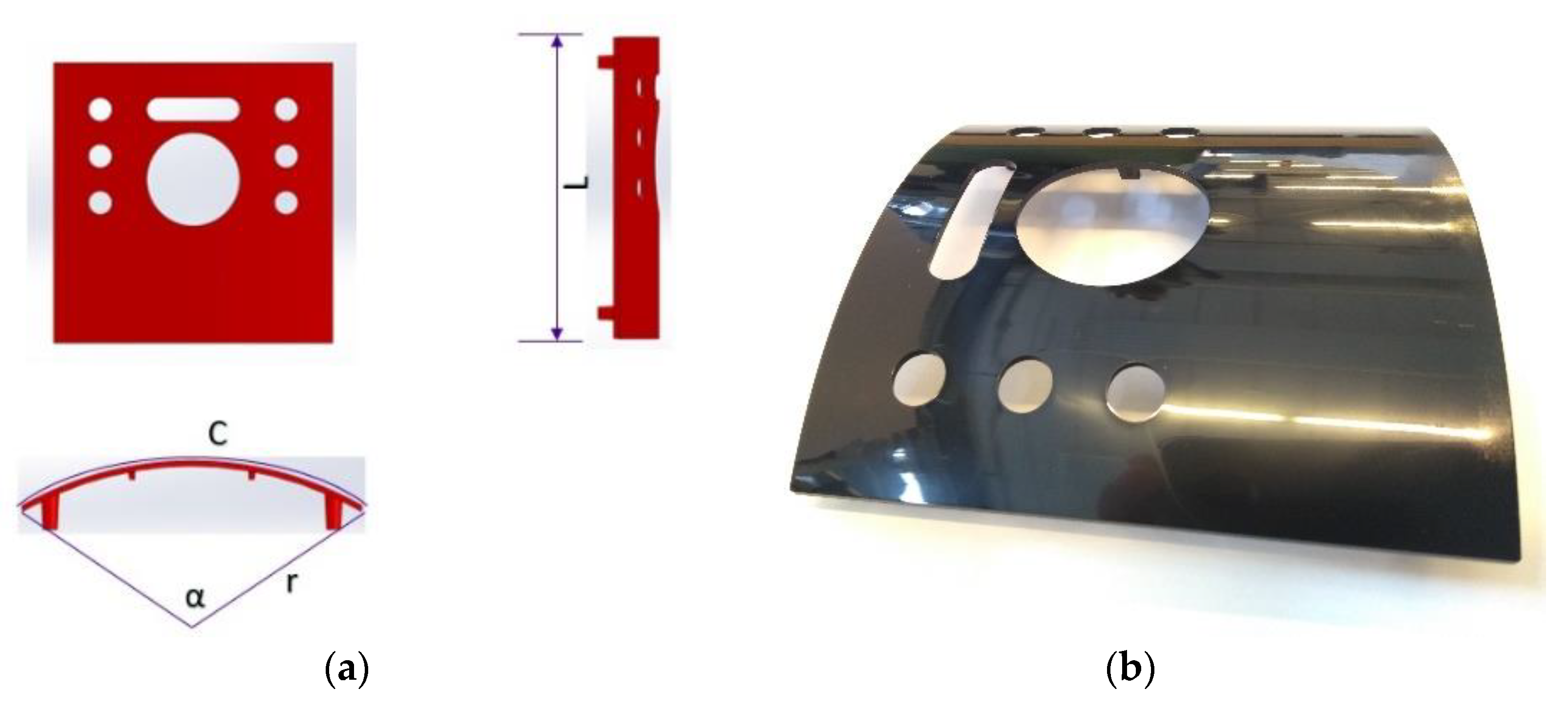
2.1. Part Properties

The inspected part is a partially cylindrically shaped sample with mold dimensions of length (L) = 120.2 mm, outer radius (r) = 123 mm, curve (bow) length (C) = 125.36 mm, and arc angle (α) = 58.39°, as illustrated in Figure 1a. The dimensional properties after ejection of the part from the mold vary depending on its shrinkage and warpage originating from the employed material, process parameters, and geometric features of the part. The post-molded volumetric shrinkage ratio for ABS (acrylonitrile butadiene styrene, i.e., the selected material) is approximately 0.4 to 0.7% [36]. Therefore, the part dimensions, after complete shrinkage for more than 24 h, are expected to be L = 119.4–119.7 mm, r = 122.1–122.5 mm, and C = 124.5–124.9 mm. Warpage is measured as the deviation from centroid shrinkage, i.e., as deviation from the mean radius.

The highly reflective surface of the part, as illustrated in Figure 1b, makes optical measurement challenging with respect to the optical dimensional measurement and surface defects. The combination of cylindricality, high reflectivity, and black color makes the measurement problem a difficult case for conventional optical measurement methods.

2.2. Measurement Requirements

Based on initial simulations of the injection molding process for this part, the minimum required resolution of the measurement should be ±5 µm to detect the effects of all studied injection molding process parameters on dimensions of the produced part. Accordingly, the goal of our research is to achieve such precision for maximum traceability of the effects of the process parameters.

2.3. Part Manipulation: Gripper

A Kuka^® KR 5 arc (KUKA CEE GmbH, Steyregg, Austria) robot is responsible for delivering the produced parts from the opened injection mold to the measurement system, completing the in-line measurement, and assuring time consistency between production and measurement. The handling system for the part should avoid any dimensional distortion before shrinkage and warpage measurements, as well as any surface intervention, to avoid disturbing sink marks and weld line detections. Therefore, the central circular hole of the part is used for handling between the mold and the fixture in the measurement system. The handling method is demonstrated in Figure 2a. The gripper is designed with a conical shape to provide maximal surface contact with the part and reduce the force and, consequently, the strain on the part (Figure 2b).

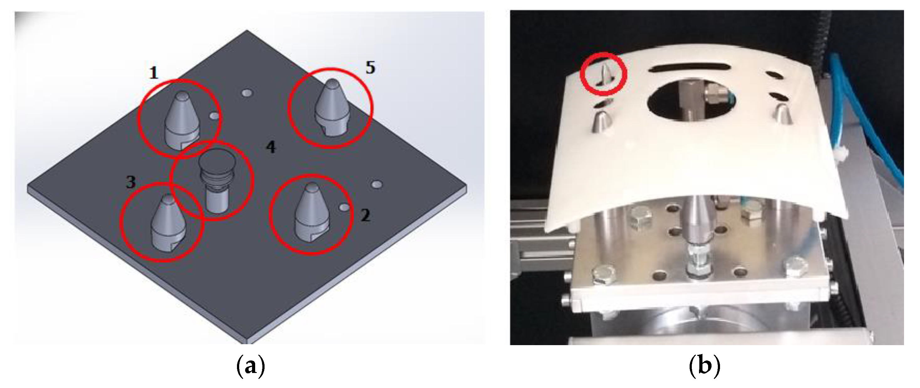
2.4. Fixture on the Measurement Stations

A fixture (Figure 3) mounted on the dimensional measurement system protects the part against unwanted movements during the measurements. The fixture must avoid any surface or dimensional distortion. Therefore, a fixture with four support pins and one vacuum suction cup was designed. The functions of the fixture parts (see Figure 3a) are as follows:

Pins 1 and 2 Fix the part through the lowest small eccentric holes in its surface against rotations and surface movements, limiting the downward movement of the part.

Pin 3 limits the downward movement and rotation of the part.

Pin 5 prevents the part from falling down when the vacuum suction is turned off.

The needle pin (highlighted in Figure 3b) is used to prevent positioning of the part in the incorrect direction on the fixture during troubleshooting by manual operation.

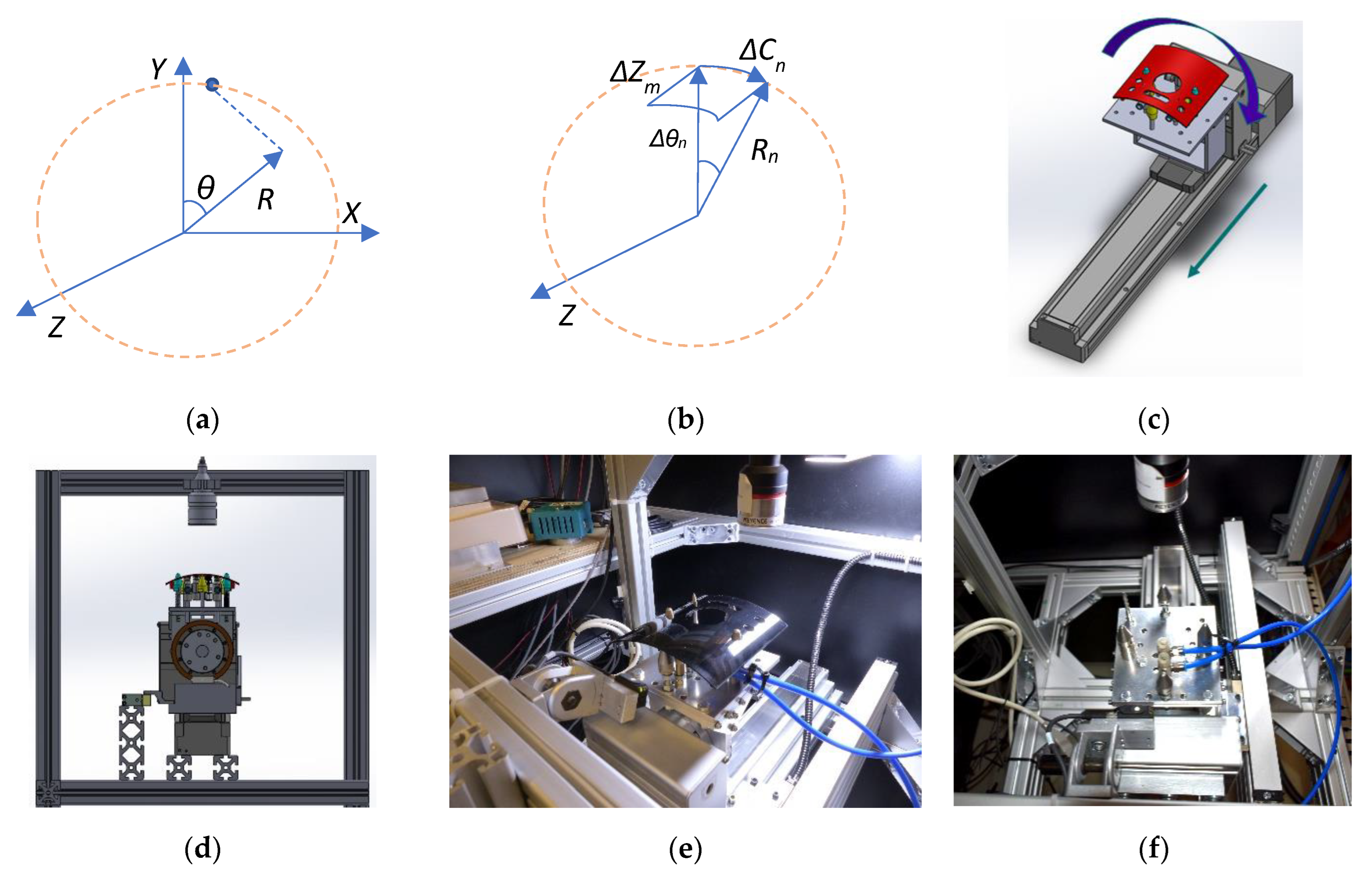
3. Measurement System and Experiments

3.1. Feasibility Test

The confocal principle uses focused light emanating from an aperture onto the object to detect the light reflected from the object back into the aperture. The source light is transmitted using an optical fiber to the measurement head lens, which emits light at varying focal distances for each wavelength. The light reflected from the target surface passes through the lens into the spectrometer. The received light is split by wavelength and focused onto a high-resolution image sensor. Finally, a processor calculates the distance to the target based on the received light signals on the image sensor using processing techniques [22,24,25]. There are various types of optical measurement sensors; we initially studied those produced by KEYENCE company. In the interest of brevity, the results are not presented in this paper. Based on the results of the initial experiments, a CL-3000 series confocal displacement sensor with a CL-P070 head [28] (KEYENCE INTERNATIONAL, Salzburg, Austria) was selected because of its appropriate response on black convex mirrored surfaces, its wide response range, high accuracy, and small laser spot diameter. Additionally, the selected CL sensor head type eliminates excess heat generation at the sensor head, which is important for high-precision measurement with confocal sensors [29]. The spot diameter of the laser head is 50 µm, and the output resolution is 0.25 µm; a resolution of 1.0 µm was selected in the controller for the output declaration. The linearity of the output within a range of ±3.0 mm is ±2.0 µm, and the maximum sampling rate of the laser controller is 10 kHz [28].

We initially expected that a two-dimensional linear system should be able to scan the part surface while moving the part under the confocal laser sensor. However, during the experiments, we observed that the confocal laser sensor was not able to read the reflection of the mirror surface at angle of more than 20 degrees. Therefore, about 17 mm of each side of the part (Figure 4) could not be measured by the confocal laser sensor with linear movements only, resulting in the conclusion that a fully Cartesian measurement system is not feasible.

3.2. Measurement Methodology

The adopted solution for non-contact measurement of the part involves rotating the part around its cylindrical center, i.e., the measured surface section is always perpendicular to the sensor axis. Linear and rotary scans should be performed for 3D measurement of the surface of the part (shown in Figure 5c,d). Three-dimensional measurement consists of the relative rotated angle (θ), the relative position of linear movement (Z), and the measured radius of the surface element (R) (Figure 5a,b). For synchronization of the R, θ, and Z measurements, one linear encoder and one rotary encoder are used to provide pulse commands to the confocal sensor for sampling. The confocal controller takes one sample as soon as it receives a pulse command on the encoder input card. The stored values in the confocal controller for points that are beyond the part surface are represented by maximum values, whereas points on the part surface are represented by values in the range of ±3000 µm. The linear length of the measurement is determined by the number of scan points on the sample surface during the linear scan and the resolution value of the linear encoder in one pulse. Similarly, the arc length of the sample depends on the number of rotary encoder pulses and the measured radius (R) at the scan point.

The linear encoder is a FAGOR ‘MX-420’ with 1µm resolution and 5µm accuracy. The rotary encoder is an RLS magnetic encoder with an ‘LM13IC2D0AA50F00’ head with a resolution of 1 µm and a max scan frequency of 8 MHz, in addition to an ‘MR100S071A152B00’ disk with a 100 mm diameter and 152 poles, with a pole length of 2 mm. The rotary encoder provides 304,000 pulses per revolution (PPR) in A-B mode, and the linear encoder nominally provides 1000 pulses per millimeter (PPM).

The sampling speed of the confocal sensor is 10 kHz, and a divider is applied to reach the cycle time limit with a 5 µm resolution in the Z (divided by 5) and arc direction (divided by 2). The arc length of the sample in the design is 125.36 mm, which was expected to be in the range of 124.5 to 124.9 mm and is equivalent to a maximum of 24,980 steps for a resolution of 5 µm. The angle of the sample arc is approximately 60° (58.36°), which comprises 149,880 steps for a complete revolution (PPR). The closest value to the required PPR is half of the encoder output, i.e., 152,000 PPR, which is provided by using a pulse divider to be divided by two.

Based on the given descriptions and Figure 5b, the following applies:

$$Z={\displaystyle \sum }_m\Delta Z_m=m\times \Delta Z$$

(1)

$$C={\displaystyle \sum }_n{R}_n\times \Delta {\theta }_n={\displaystyle \sum }_n{R}_n\times \Delta \theta$$

(2)

where ΔZ_m is the length value for each encoder pulse to the confocal sensor in the Z direction through linear movements, which nominally equals ΔZ = 0.005 mm per pulse for all of the m points of sampling in the Z direction. Subsequently, Δθ_n is the rotation angle value for each encoder pulse to the confocal sensor during the rotary movements, which nominally equals Δθ = 0.00236842° per pulse for all n sampling points. The nominal curve length (ΔC) for each rotation element is:

$$\Delta C=122.56\times 0.00236842\times \frac{pi}{180}=0.005066 \mathrm{mm}$$

(3)

where the radius of the designed part is 123 mm, which is expected to be 122.1 to 122.5 mm after shrinkage. During the rotation, the actual radius (R_n) differs depending on the local (shrinkage- and warpage-induced) radial deviation of the surface element. R_n includes a constant distance from the rotation center of the rotary axis to the zero position of the confocal sensor, i.e., R₀ = 122.56, and the distance measured by the confocal sensor (R_CL,n) from the zero position of the confocal sensor.

R_n = R₀ + R_CL,n

(4)

Therefore, the arc length of the part can be measured as (keeping in mind that $\Delta {\theta }_n=\Delta \theta$):

$$C={\displaystyle \sum }_n{R}_n\times \Delta \theta ={\displaystyle \sum }_n\left(R_0+R_{C{L}_n}\right)\times \Delta \theta ={\displaystyle \sum }_n{R}_{C{L}_n}\times \Delta \theta +n\times R_0\times \Delta \theta$$

(5)

Because the total measurement duration should be less than the molding cycle time, it would be impossible to perform a complete scan of the surface of the part. Hence, three linear and three rotary lines on the samples are measured as illustrated in Figure 6. The four close-to-corner lines are positioned approximately above the center of the backside screw pins, allowing for a future study on sink marks measurements in these areas. The other two lines are approximately positioned at the center of the part and the center of the large circular hole, respectively. Later, the dimension of each line will be compared with similar lines of the other samples (or the golden sample) to observe shrinkage alterations. Warpage is defined based on the shrinkage balance between scanned profiles of the samples.

We used linear and rotary units from SMC company (SMC Austria GmbH, Korneuburg, Austria). The linear drive is an “LEFSH40B-300-R5CE17” series, and the rotary drive is an “LERH50K” series. The applied vacuum suction actuator exhibits a minimum load/displacement error in the design and fixture load. The nominal positioning accuracy of the actuators is ±0.01 mm for the linear and ±0.03° for the rotary axis. Although the accuracies of the actuators do not match with the target precision of the measurements, the precision of the measurements is obtained by the encoders and the confocal sensor sampling. Precise positioning of the axes is required to position the scan lines and home position for coworking with the pick–place robot. The scan line movements start from an absolute position (based on the axes coordinates and accuracies) outside the injection-molded part. The rotary unit moves to the absolute positions of 17.25°, 40.00° (center), and 65.30° angles for linear scans, starting from the absolute linear position of 30.00 mm and running to the absolute linear position of 160.00 mm. Subsequently, the linear axis moves to the 49.05 mm, 88.00 mm, and 147.50 mm positions for a rotated scan starting from 5.00° to 75.00° angles.

A BECKHOFF^® IPC modelCP6600 (BECKHOFF Automation GmbH, Buers, Germany) was programmed to control axes movements and communicate with the robot and software (running on a separate computer for data acquisition) to read and store the data from the confocal sensor controller. The robot takes the part from the opened mold, checks the orientation of the part (for a possible rotation during the ejection and picking process) in a fork sensor, places the part on the balance, and finally, places the part on the fixture of the presented dimensional measurement system (see also Figure 7). Moreover, the time difference between the production and measurement is recorded (30 to 32 s); parts with excess time difference are excluded from the final shrinkage/warpage comparison due to time-dependent shrinkage.

The communication between the injection molding machine, IPC, and the data acquisition computer (DAQ) takes place on the OPC UA platform, as shown in Figure 8. The actual part number of the molded part, along with the production time, is extracted from the injection molding machine over OPC UA. Simultaneously, the time of measurement is read from the IPC and stored. The raw measurement data of the confocal sensor is stored on the DAQ computer for every point, including the pulse count number (received from the linear or rotary encoder) and the height distance from the confocal zero position of the sensor. A program written in Python code calculates the length of the scanned lines for each molded part after each measurement cycle.

3.3. Experiment 1: Precision Validation Using a Self-Built Gauge

A special gauge (Figure 9) was built to test the repeatability and precision of the built system. The test measurements were conducted without encoders; therefore, a different scan strategy was adopted. Three linear scans at various angles and three rotary scans at different longitudinal positions were performed on the gauge (shown in Figure 9). The axes speeds were selected to as 30, 60, and 120 mm/s for linear scans and 30 and 60°/s for rotary scans (shown in

Table 1. Experiments performed for repeatability evaluation.

Exp.	Position	Type	Speed	Unit
1-1	PL1	Linear	30	mm/s
1-2	PL1	Linear	60	mm/s
1-3	PL1	Linear	120	mm/s
1-4	PL2	Linear	30	mm/s
1-5	PL2	Linear	60	mm/s
1-6	PL2	Linear	120	mm/s
1-7	PL3	Linear	30	mm/s
1-8	PL3	Linear	60	mm/s
1-9	PL3	Linear	120	mm/s
1-10	RP1	Rotary	30	°/s
1-11	RP1	Rotary	60	°/s
1-12	RP2	Rotary	30	°/s
1-13	RP2	Rotary	60	°/s
1-14	RP3	Rotary	30	°/s
1-15	RP3	Rotary	60	°/s

). The linear scans have a length of 100 mm, and the rotary scans have a bow length of 200°. Each scan position was measured five times in both directions with similar test conditions, such as ambient temperature and environmental noise. The confocal sensor was set to a sampling frequency of 1kHz (to cover all speeds). We compared the measurements obtained with each measurement position separately to exclude systematic errors in the measurements [32].

The raw results of experiments 1–4 (linear scan for PL1 at a speed of 30 mm/s) are presented in Figure 10. Each scan took about 3.5 s at this speed, and there was a delay of 2 to 5 s due to manual movement commands. All the scans were stored continuously, and later, an algorithm based on the line slope was applied to identify the beginning of the scan lines (blue vertical lines in Figure 10). Results showed that the gauge, including the axes and production error, was tilted to a depth of about 0.03 mm with a length of 100 mm (about 0.017°). The scans in the reverse movement direction were rotated, and the ends of all scans were cut, resulting in the same length after extraction. To evaluate the repeatability of the measurements, the measurement values were subtracted from the average of the measurements, once considering only unidirectional movement and once considering only bidirectional movements, in order to compare the deviations of the scans and therefore the repeatability of the measurements. The comparison results and a histogram of the error are presented in Figure 11.

The comparison of errors in the R direction shows a satisfactory unidirectional result of ±2 µm with a Gaussian distribution around the center, indicating that the error is a random type. However, a phase-shift problem occurred in the bidirectional comparison between the forward and backward directions, as shown in Figure 11b. Therefore, the measurement approach should be unidirectional for higher measurement repeatability.

The precision of the measurement system was examined using a precision gauge in this experiment. The unidirectional movements were found to be more accurate (less than 5 µm) in the confocal sensor direction, whereas the error distribution was normal. The standard deviation of the error (illustrated in Figure 12) proves the repeatability of the measurements in the sensor direction, with a maximum standard deviation of 1.15 µm for the unidirectional and 1.9 µm for bidirectional movements. Additionally, a group of similarity tests were derived to test the similarity of the measurement signals given in Figure 11a for all five unidirectional scans; the results are presented in Figure 13. The measurements similarity results show a very low RMS (root mean square) difference, and the cross-correlations between the mean of the measurements and each measurement match perfectly, which shows the best matching signal at zero lag.

3.4. Experiment 2: Precision Validation on the Molded Part

After the rotary encoder installation, 14 molded parts with different production settings were produced and sampled under stable production conditions to quantify the precision of the measurements. The produced parts were stored close to the measurement system at a temperature of about 23 °C for at least 48 h to ensure dimensional stability of the injection-molded parts. For the experiment, the parts were manually positioned on a fixture on the scale. Afterwards, the Kuka robot picked up the part from the fixture on the scale and positioned it on the fixture of the measurement system. Each part was measured 11 times continuously with a time difference of about 50 s to duplicate the in-line measurement conditions.

The measurements were compared with respect to the length and the stability in the confocal sensor direction (R). The first measurement was used as the reference, and other measurements were subtracted from the reference to observe the possible effect of the suction force. The results, illustrated for a sample in Figure 14, show that the difference from the first measurement increases with successive measurements. This effect appears strongest at the center of the part for line R1 and the corners of the part for R3 due to the positions of the support pins on the fixture, whereas the center of R3 is fixed under the support pin 3 (Figure 3) and shows no movement during the measurements. The linear line (L2) in the center rotates downward, whereas lines L1 and L3 exhibit a rotation effect combined with the deformation effect of R1 and R3. Based on the results shown in Figure 14, it can be concluded that the suction has a deformation effect of up to 10 µm in a time duration of about 9 min. The duration of the measurement for each part is about 50 s, and the total suction effect on the dimension in the first 50 s is less than 3 µm on the cooled part. However, the temperature of the as-molded part is higher; therefore, a higher deformation effect in 50 s can be expected, rather than the cooled part.

The length of the measured lines for the same sample is provided in

Table 2. The calculated length of the lines (in mm) and the error range for lines 1 to 6.

Line	Mean Val.	Min	Max	Error
R1	122.742	122.736	122.747	0.011
R2	122.943	122.940	122.948	0.008
R3	122.831	122.822	122.834	0.012
L1	119.704	119.700	119.710	0.010
L2	119.785	119.780	119.790	0.010
L3	119.657	119.660	119.655	0.005

. Despite the suction deformation effect during the 9 min of measurement, the maximum error for the length of linear lines fits in ±5 µm. However, the maximum error for the length of rotary lines is ±6 µm. The number of encoder pulses from the starting absolute position of the dimensional measurement system to the detected edge of the part for each scan line is given in

Table 3. The distance (number of encoder pulses) from the starting absolute point to the part edge for each line.

Distance to Line	Min	Max	Difference
R1	2488	2490	2
R2	2492	2494	2
R3	2474	2477	3
L1	425	426	1
L2	414	416	2
L3	383	384	1

.

The experiment was conducted on 14 parts produced under different machine settings. The results show a difference of a maximum of ±10 µm for the length of the lines (Figure 15) and a maximum pulse difference of ±2 for the distance from the absolute starting point (Figure 15a). However, this error includes the deformation resulting from the suction force, which was applied for 9 min duration of the successive measurement. The result of this experiment shows that the measurement repeatability error of the presented measurement system is better than ±10 µm for the presented measuring part, despite the repeatability error for most of the measurements being limited to ±5 µm. Results for the distance from absolute starting point to the edge of the part is shown in Figure 16.

3.5. Experiment 3: Positioning Error on the Fixture

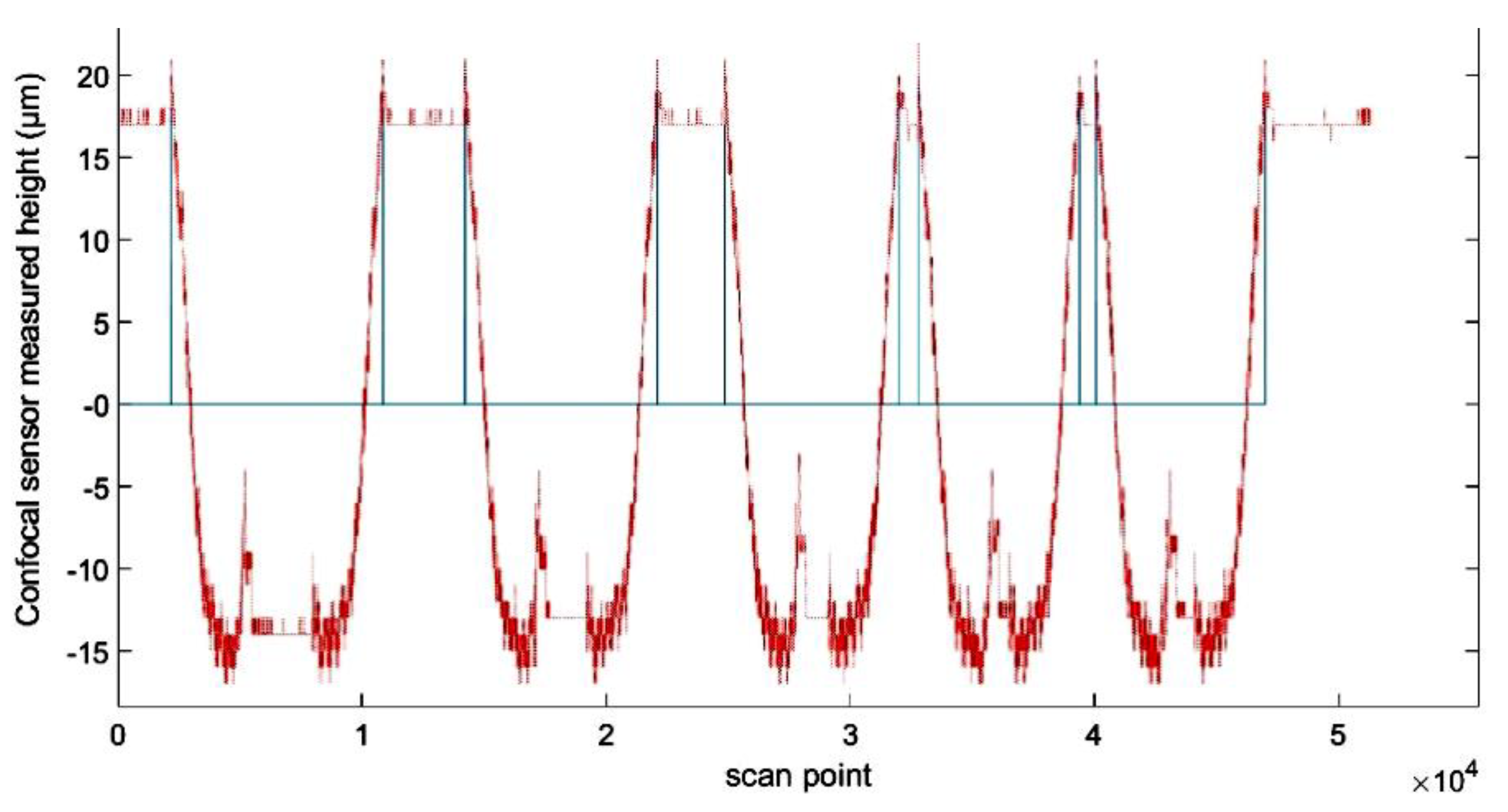
After the robot positions the part on the fixture and releases it, the suction forces the part down onto the fixture, and the part settles through the fixture pins (Figure 3, pins 2 and 4). Several factors, such as the shrinkage of the holes of the pin positions and friction between the part surface and the pins, influence the part settlement. Further study of the errors of part positioning on the fixture is needed to perceive the error sources and possible required modifications.

Six types of minor part movements can occur on the fixture, as shown in Figure 17. Positioning errors ‘a’ and ‘f’ do not affect the results of the measurement. Errors ‘b’ and ‘e’ affect the length of linear and rotary lines. These errors can be calculated based on the distance from the absolute starting point to the edge of the part. Errors ‘c’ and ‘d’, in particular, affect the length of the rotary lines. Therefore, further study is required with respect to the level of these errors and the effect on the line length.

A set of 10 parts is selected with different machine settings after the stability of the production is verified. The robot places each part on the measurement system 13 times. It picks up the part after finishing the measurement each time and replaces the part on the measurement system to conclude the experiment. The first scan is considered the reference, and other scans are subtracted from the first scan to observe deviations during the successive replacements and scans.

The results of the replacement of the part for one sample are illustrated in Figure 18. The selected sample has moved between 15 and 30 µm in all directions (based on the distance from the absolute starting point). The R direction shows the movements of the sample included with the deformation resulting from the suction force. The effects of replacement are as large as ±40 µm (although mostly ±20 µm) in some scans in the R direction. The error of the distance to the edge of the part and the error of the line length for all parts remain within ±10 µm tolerance.

4. Results

Three experiments were carried out for precision validation of the presented cylindrical dimensional measurement system. Each experiment validated some properties of the measurement system. Experiment 1 validated the R direction (confocal sensor direction) during linear and rotary movements. A list of experiments is given in Table 1. The variation range of the standard deviation during each experiment is illustrated in Figure 12. The standard deviation of the errors (Figure 12) shows that the error of the linear movement increases with the increment of the speed for experiments 1 to 9 (linear movements), whereas the error decreases with the increment of the speed for experiments 10 to 15 (rotary movements). Moreover, Figure 12 shows that the error for bidirectional movements is higher than the error for unidirectional movements. Although the error is in the boundary of ±5 µm, the bidirectional movements are rejected, and unidirectional movements are accepted for higher precision. To test the results of scans with respect to additional aspects, the mean square error (MSE), structural similarity index (SSIM), root mean square (RMS) level, and cross correlation between the mean of the measurements and each measurement were calculated as the measures of signal similarity. The results for experiments 1–4 are presented in Figure 13. The high similarity index, very low MSE error, and very low RMS difference indicate that measurements are close to each other. The matching cross correlations between the mean of the signals and each signal with a central peak at zero and a value of 0.9998 is another measure to validate the similarity of the measurements. These measures were repeated for the other experiments, with similar results for both unidirectional movements.

Experiment 2 showed the actual repeatability error of the dimensional measurement system with the in-line conditions, despite the effect of the suction force in the R direction. The results are given in Figure 15 and Figure 16. This experiment was conducted on 14 samples with different machine settings. Figure 15 shows the variations in the line length and error distribution versus the variation in machine settings. We expected that all lines would approximately follow a similar gradient. Because Line 3 did not follow the rule, we investigated and found a flashing problem on the end side of the line. The error tolerance for most of the samples is below ±5 µm. However, for some samples, the error increases up to ±10 µm. Regarding the deformation caused by suction force, the large error could be a result of increased deformation (lower stiffness) during the 9 min of measurement.

The distance from the absolute starting point of each line to the part edge is given in Figure 16. This distance is useful for reshaping the three-dimensional part for shrinkage and warpage calculations. The distance to Line 1 (DL1) has a larger error tolerance than the other lines, as the position of Line1 on the part has the largest distance to the support pins on the fixture. The error tolerance of the distance to the edge of the part for most of the lines fits in the range of ±5 µm; however, the error tolerance for all the measurements and lines fits in the range of ±10 µm.

With experiment 3, we studied the error produced by the fixture during placement of the part by the robot. The results show a displacement of ±20 µm in the R direction during the replacement of the part on the fixture. The linear lines are less sensitive to the replacement, whereas the rotary lines seem to be very sensitive. The middle of Line 3 (R3), which is fixed on support pin 3, is a very repeatable point of measurement. Despite the displacement error and the suction force effect, the tolerance of the line length fits within ±10 µm for all the measurements.

5. Conclusions

The final result shows that the repeatability of the scans in the R direction is dependent on the speed of movement, although the signal similarity error is always less than ±5 µm. The repeatability experiments with the injection-molded part show that the total precision of the measurement system is around ±5 µm for a short period of measurement (under 60 s). However, the suction force and slight movement of the part increase the error to a value of a maximum of ±10 µm.

In addition to the suction force, positioning the part on the fixture includes multiple errors, which have a minor influence on the part dimensional measurement and a major influence on the absolute positioning of the part in the cylindrical coordinate system.

In this study, the zero-position radius of the confocal sensor was calculated experimentally. For a future system generalization, we plan to develop an algorithm that automatically determines the zero-position radius. Moreover, we will build a new fixture to reduce the suction effect on the part and increase the precision of the measurements.

References

1. Ahmed, T.; Sharma, P.; Karmaker, C.L.; Nasir, S. Warpage Prediction of Injection-Molded PVC Part Using Ensemble Machine Learning Algorithm. Mater. Today Proc. 2020. [Google Scholar] [CrossRef]
2. Singh, G.; Pradhan, M.K.; Verma, A. Multi Response Optimization of Injection Moulding Process Parameters to Reduce Cycle Time and Warpage. Mater. Today Proc. 2018, 5, 8398–8405. [Google Scholar] [CrossRef]
3. Gruber, D.P.; Buder-Stroisznigg, M.; Wallner, G.; Strauss, B.; Jandel, L.; Lang, R.W. A Novel Methodology for the Evaluation of Distinctness of Image of Glossy Surfaces. Prog. Org. Coat. 2008, 63, 377–381. [Google Scholar] [CrossRef]
4. Gruber, D.P. Method for Automatically Detecting a Defect on a Surface of a Molded Part. WO2010102319, 16 September 2010. [Google Scholar]
5. Gruber, D.P.; Buder-Stroisznigg, M.; Wallner, G.; Strauß, B.; Jandel, L.; Lang, R.W. Characterization of Gloss Properties of Differently Treated Polymer Coating Surfaces by Surface Clarity Measurement Methodology. Appl. Opt. 2012, 51, 4833–4840. [Google Scholar] [CrossRef]
6. Gruber, D.P. Method and Device for the Optical Analysis of the Surface of an Object. EP14186013, 1 April 2015. [Google Scholar]
7. Masato, D.; Rathore, J.; Sorgato, M.; Carmignato, S.; Lucchetta, G. Analysis of the Shrinkage of Injection-Molded Fiber-Reinforced Thin-Wall Parts. Mater. Des. 2017, 132, 496–504. [Google Scholar] [CrossRef]
8. Sreedharan, J.; Jeevanantham, A.K. Analysis of Shrinkages in ABS Injection Molding Parts for Automobile Applications. Mater. Today Proc. 2018, 5, 12744–12749. [Google Scholar] [CrossRef]
9. Azad, R.; Shahrajabian, H. Experimental Study of Warpage and Shrinkage in Injection Molding of HDPE/RPET/Wood Composites with Multiobjective Optimization. Mater. Manuf. Processes 2019, 34, 274–282. [Google Scholar] [CrossRef]
10. Barghash, M.A.; Alkaabneh, F.A. Shrinkage and Warpage Detailed Analysis and Optimization for the Injection Molding Process Using Multistage Experimental Design. Qual. Eng. 2014, 26, 319–334. [Google Scholar] [CrossRef]
11. Chen, W.-C.; Fu, G.-L.; Tai, P.-H.; Deng, W.-J.; Fan, Y.-C. ANN and GA-Based Process Parameter Optimization for MIMO Plastic Injection Molding. In Proceedings of the 2007 International Conference on Machine Learning and Cybernetics, Hong Kong, China, 19–22 August 2007; Volume 4, pp. 1909–1917. [Google Scholar] [CrossRef]
12. Ozcelik, B.; Erzurumlu, T. Comparison of the Warpage Optimization in the Plastic Injection Molding Using ANOVA, Neural Network Model and Genetic Algorithm. J. Mater. Process. Technol. 2006, 171, 437–445. [Google Scholar] [CrossRef]
13. Petrova, T.; Kazmer, D. Hybrid Neural Models for Pressure Control in Injection Molding. Adv. Polym. Technol. 1999, 18, 19–31. [Google Scholar] [CrossRef]
14. Kazmer, D.O. Injection Mold Design Engineering. In Injection Mold Design Engineering, 2nd ed.; Kazmer, D.O., Ed.; Hanser Publishers: Munich, Germany, 2016; pp. I–XXIV. ISBN 978-1-56990-570-8. [Google Scholar]
15. Liao, S.J.; Chang, D.Y.; Chen, H.J.; Tsou, L.S.; Ho, J.R.; Yau, H.T.; Hsieh, W.H.; Wang, J.T.; Su, Y.C. Optimal Process Conditions of Shrinkage and Warpage of Thin-Wall Parts. Polym. Eng. Sci. 2004, 44, 917–928. [Google Scholar] [CrossRef]
16. Jansen, K.M.B.; Van Dijk, D.J.; Husselman, M.H. Effect of Processing Conditions on Shrinkage in Injection Molding. Polym. Eng. Sci. 1998, 38, 838–846. [Google Scholar] [CrossRef]
17. Pomerleau, J.; Sanschagrin, B. Injection Molding Shrinkage of PP: Experimental Progress. Polym. Eng. Sci. 2006, 46, 1275–1283. [Google Scholar] [CrossRef]
18. Régnier, G.; Trotignon, J.P. Local Orthotropic Shrinkage Determination in Injected Moulded Polymer Plates. Polym. Test. 1993, 12, 383–392. [Google Scholar] [CrossRef]
19. Gao, J.; Gindy, N.; Chen, X. An Automated GD&T Inspection System Based on Non-Contact 3D Digitization. Int. J. Prod. Res. 2006, 44, 117–134. [Google Scholar] [CrossRef]
20. Liu, Y.; Zhang, Q.; Liu, Y.; Yu, X.; Hou, Y.; Chen, W. High-Speed 3D Shape Measurement Using a Rotary Mechanical Projector. Opt. Express 2021, 29, 7885–7903. [Google Scholar] [CrossRef]
21. Li, W.; Zhou, L.; Yan, S.-J. A Case Study of Blade Inspection Based on Optical Scanning Method. Int. J. Prod. Res. 2015, 53, 2165–2178. [Google Scholar] [CrossRef]
22. Alkmal, J.S. Investigation of Optical Distance Sensors for Applications in Tool Industry: Optical Distance Sensors. Master’s Thesis, Saimaa University of Applied Science, South Kariland, Finland, 2013. [Google Scholar]
23. Boltryk, P.J.; Hill, M.; McBride, J.W.; Nascè, A. A Comparison of Precision Optical Displacement Sensors for the 3D Measurement of Complex Surface Profiles. Sens. Actuators A Phys. 2008, 142, 2–11. [Google Scholar] [CrossRef]
24. Jordan, H.-J.; Wegner, M.; Tiziani, H. Highly Accurate Non-Contact Characterization of Engineering Surfaces Using Confocal Microscopy. Meas. Sci. Technol. 1998, 9, 1142–1151. [Google Scholar] [CrossRef]
25. Yang, L.; Wang, G.; Wang, J.; Xu, Z. Surface Profilometry with a Fibre Optical Confocal Scanning Microscope. Meas. Sci. Technol. 2000, 11, 1786–1791. [Google Scholar] [CrossRef]
26. Yang, Y.; Dong, Z.; Meng, Y.; Shao, C. Data-Driven Intelligent 3D Surface Measurement in Smart Manufacturing: Review and Outlook. Machines 2021, 9, 13. [Google Scholar] [CrossRef]
27. Nouira, H.; El-Hayek, N.; Yuan, X.; Anwer, N.; Salgado, J. Metrological Characterization of Optical Confocal Sensors Measurements (20 and 350 Travel Ranges). J. Phys. Conf. Ser. 2014, 483, 012015. [Google Scholar] [CrossRef]
28. Keyence Confocal Displacement Sensors CL-3000. 2019. Available online: www.keyence.com (accessed on 24 March 2019).
29. Berkovic, G.; Zilberman, S.; Shafir, E. Temperature Effects in Chromatic Confocal Distance Sensors. In Proceedings of the SENSORS, 2013 IEEE, Baltimore, MD, USA, 3–6 November 2013; pp. 1–3. [Google Scholar] [CrossRef]
30. Geometrical Product Specifications (GPS)—Roundness 2011, no. ISO12181-2. Available online: https://www.iso.org/standard/53621.html (accessed on 20 March 2021).
31. Geometrical Product Specifications (GPS)—Geometrical Tolerancing—Tolerances of Form, Orientation, Location and Run-Out, 2017, no. ISO1101. Available online: https://www.iso.org/obp/ui/#iso:std:iso:1101:ed-4:v1:en (accessed on 20 March 2021).
32. Sun, C.; Wang, H.; Liu, Y.; Wang, X.; Wang, B.; Li, C.; Tan, J. A Cylindrical Profile Measurement Method for Cylindricity and Coaxiality of Stepped Shaft. Int. J. Adv. Manuf. Technol. 2020, 111, 2845–2856. [Google Scholar] [CrossRef]
33. Zeng, W.; Jiang, X.; Scott, P.J. Roundness Filtration by Using a Robust Regression Filter. Meas. Sci. Technol. 2011, 22, 035108. [Google Scholar] [CrossRef]
34. Gosar, Z.; Gruber, D.P. IN-LINE Quality Inspection of Freeform Plastic High Gloss Surfaces Aided by Multi-Axial Robotic Systems. In Proceedings of the International Electrotechnical and Computer Science Conference (ERK’2017), Portotoz, Slovenia, 26 September 2017; pp. 445–448. [Google Scholar]
35. Chiariotti, P.; Fitti, M.; Castellini, P.; Zitti, S.; Zannini, M.; Paone, N. High-Accuracy Dimensional Measurement of Cylindrical Components by an Automated Test Station Based on Confocal Chromatic Sensor. In Proceedings of the 2018 Workshop on Metrology for Industry 4.0 and IoT, Brescia, Italy, 16–18 April 2018; pp. 58–62. [Google Scholar] [CrossRef]
36. Brinkmann, O.B.; Schmachtenberg, O. International Plastics Handbook; HANSER: Munich, Germany, 2012; pp. 547–553. [Google Scholar]
Figure 1. Illustration of the measurement sample. (a) Isometric view of the sample. (b) The highly reflective surface of the sample, called a piano-black surface.
Technologies 10 00095 g001
Figure 2. The robot handling gripper. (a) Picking up the part through its center hole. (b) Matching the gripper slope with the hole slope for surface contact.
Technologies 10 00095 g002
Figure 3. Illustration of the measurement station fixture. (a) Positions of Support pins 1, 2, 3, 5 and vacuum suction 4. (b) A part positioned on the fixture.
Technologies 10 00095 g003
Figure 4. A local surface slope of more than 20° hindered the confocal sensor from achieving proper measurement, i.e., about 17 mm from either edge inward was unmeasurable with pure linear movements of the part under the sensor.
Technologies 10 00095 g004
Figure 5. The final measurement system design. (a) Cylindrical coordinate system; (b) movement details during measurement; (c) two-dimensional movements; (d) side view of the rotary unit and confocal head; (e) isometric view of the installed dimensional measurement system; (f) top view of the installed dimensional measurement system.
Technologies 10 00095 g005
Figure 6. The position of the six scanning lines.
Technologies 10 00095 g006
Figure 7. The handling and measurement procedure of the injection-molded part.
Technologies 10 00095 g007
Figure 8. OPC UA communication platform between the IPC, injection molding machine, and data acquisition computer.
Technologies 10 00095 g008
Figure 9. (a) The designed gauge for initial precision validation and (b) the gauge installed on the axis.
Technologies 10 00095 g009
Figure 10. Raw result of confocal scan at the PL1 position with a speed of 30 mm/s.
Technologies 10 00095 g010
Figure 11. Five PL1 scans with a speed of 30 mm/s are subtracted from the average value: (a) unidirectional movements; (b) bidirectional movements; (c) histogram of error distribution for unidirectional movements; (d) histogram of error distribution for bidirectional movements.
Technologies 10 00095 g011
Figure 12. Standard deviation of errors for experiment 1 tests. (a) Standard deviation of errors for unidirectional movements; (b) standard deviation of errors for bidirectional movements.
Technologies 10 00095 g012
Figure 13. Similarity measures, (a) RMS level, (b) MSE error, (c) SSIM in percentage, and (d) cross correlation between the mean of measurements and each measurement.
Technologies 10 00095 g013
Figure 14. The difference of the scan lines between the first and the next 10 lines indicates the suction force effect during the successive measurements.
Technologies 10 00095 g014
Figure 15. (a) Average measured line length for 14 samples. (b) Repeatability error range for the 14 samples.
Technologies 10 00095 g015
Figure 16. (a) Distance from the absolute starting point for the 14 samples. (b) Repeatability error range for the distance to the starting point.
Technologies 10 00095 g016
Figure 17. The six types of possible positioning errors of the part on the fixture.
Technologies 10 00095 g017
Figure 18. Repositioning of the part on the fixture in the R direction. The next 12 scans are subtracted from the first scan for comparison.
Technologies 10 00095 g018