Article

Traffic Flow Prediction for Smart Traffic Lights Using Machine Learning Algorithms

by
Alfonso Navarro-Espinoza
1,
Oscar Roberto López-Bonilla
1,
Enrique Efrén García-Guerrero
1,
Esteban Tlelo-Cuautle
2,
Didier López-Mancilla
3,
Carlos Hernández-Mejía
4 and
Everardo Inzunza-González
1,*
1
Facultad de Ingeniería, Arquitectura y Diseño, Universidad Autónoma de Baja California, Carret. Transpeninsular Ensenada—Tijuana No. 3917, Fracc. Playitas, Ensenada C.P. 22860, Mexico
2
Department of Electronics, National Institute of Astrophysics, Optics and Electronics (INAOE), Puebla C.P. 72840, Mexico
3
Centro Universitario de Los Lagos, Universidad de Guadalajara (UDG), Lagos de Moreno C.P. 47460, Mexico
4
Instituto Tecnológico Superior de Misantla, Doctorado en Ciencias de la Ingeniería, Km 1.8 Carretera Lomas del Cojolite, Misantla C.P. 93821, Mexico
*
Author to whom correspondence should be addressed.
Technologies 2022, 10(1), 5; https://doi.org/10.3390/technologies10010005
Submission received: 29 November 2021 / Revised: 24 December 2021 / Accepted: 4 January 2022 / Published: 10 January 2022
(This article belongs to the Section Information and Communication Technologies)

Abstract

:
Nowadays, many cities have problems with traffic congestion at certain peak hours, which produces more pollution, noise and stress for citizens. Neural networks (NN) and machine-learning (ML) approaches are increasingly used to solve real-world problems, overcoming analytical and statistical methods, due to their ability to deal with dynamic behavior over time and with a large number of parameters in massive data. In this paper, machine-learning (ML) and deep-learning (DL) algorithms are proposed for predicting traffic flow at an intersection, thus laying the groundwork for adaptive traffic control, either by remote control of traffic lights or by applying an algorithm that adjusts the timing according to the predicted flow. Therefore, this work only focuses on traffic flow prediction. Two public datasets are used to train, validate and test the proposed ML and DL models. The first one contains the number of vehicles sampled every five minutes at six intersections for 56 days using different sensors. For this research, four of the six intersections are used to train the ML and DL models. The Multilayer Perceptron Neural Network (MLP-NN) obtained better results (R-Squared and EV score of 0.93) and took less training time, followed closely by Gradient Boosting then Recurrent Neural Networks (RNNs), with good metrics results but the longer training time, and finally Random Forest, Linear Regression and Stochastic Gradient. All ML and DL algorithms scored good performance metrics, indicating that they are feasible for implementation on smart traffic light controllers.

1. Introduction

Nowadays, the accelerated growth of the population and, consequently, the number of vehicles in the cities added to the technological limitations of traffic control signs have made vehicular traffic one of the problems of modern life. This problem has negative consequences for the environment, health and the economy.
Here is where the concept of Intelligent Transportation System (ITS) comes in, as a critical component of smart city infrastructure [1]. Using big data information and communication technology [2], ITS can provide real-time road infrastructure analysis and more efficient traffic control [3,4]. This system relies on traffic predictions as a critical component [5,6]. The purpose of traffic forecasting is to predict future traffic conditions on a transportation network based on historical observations [7]. This data can be helpful in ITS applications such as traffic congestion control and traffic light control [8]. For example, it can calculate the likelihood of congestion on the corresponding road segment and prepare for it in advance [9].
Traffic prediction can be divided into two types of techniques: parametric, including stochastic and temporal methods, and non-parametric, such as machine-learning (ML) models [10], recently used to solve complex traffic problems. The review made in [11] found that non-parametric algorithms outperform parametric algorithms due to their ability to deal with a large number of parameters in massive data. In [12] five ML algorithms are evaluated to forecast the total volume of the traffic flow in Porto city; the algorithms are: Linear Regression, Sequential Minimal Optimization (SMO) Regression, Multilayer Perceptron (MLP), M5P model tree and Random Forest (RF). The experimental results show that the M5P regression tree outperforms the other regression models. The authors in [13] reported some multi-model ML methods for traffic flow estimation from floating car data. In particular, they evaluated the capacity of Gaussian Process Regressor (GPR) to address this issue. Deep learning (DL) as a subset of ML uses multilayered neural networks exposed to many data to train themselves. This capability of DL models to extract knowledge from complex systems has made them a robust and viable solution in the field of ITS [14].
A Multilayer Perceptron Neural Network (MLP-NN) is presented in [15,16], this last with a mutual information technique to forecast traffic flow. The simulations showed a decrease in forecast error in comparison to the results of the mean and Autoregressive Integrated Moving Average (ARIMA) models that used traffic data from previous periods. Back-Propagation Neural Network (BPNN) is one of the most typical architectures of Neural Networks and is widely used in many prediction and classification tasks. In [17] an urban traffic signal control system based on traffic flow prediction using BPNN is proposed. Also [18] used BPNN to predict future traffic volumes in the design of a traffic light control system along with a genetic algorithm for timing optimization. With this method the average waiting rate is reduced by almost 30 percent compared with the fixed-time traffic light control system. Following this method, the combination of a genetic algorithm and neural network in [19] leads to a named Genetic Neural Network. Ref. [20] presents a deep learning neural network method for optimizing traffic flow and reducing congestion at key intersections by using historical data from all the movements of an intended intersection, with time series and environmental variables as the input features. The output is fed into a delay equation that generates the best green times to manage traffic delay. In [21] a short-term traffic flow prediction based on an improved wavelet neural network (WNN) is proposed. They use an improved particle swarm optimization (IPSO) to avoid being trapped in a local extremum. The outputs of the IPSO are the corresponding wavelet neural network parameters, and experimental results show that this algorithm is more efficient than the WNN and PSO–WNN algorithms alone. The prediction results are more stable and more accurate. Compared with the traditional wavelet neural network, the error is reduced by almost 15 percent.
Recurrent neural networks (RNNs) have an internal state that can represent context information; they hold information about past inputs for a period of time and are typically used to capture dynamic sequences of data. RNNs based DL methods Long Short-Term Memory (LSTM) [22], short-term flow prediction [23,24] and Gated Recurrent Units (GRU) in [25] outperform the ARIMA model; additionally, the authors report that this is the first use of GRU in traffic flow prediction. Currently, GRU models continue to be used for the development of intelligent traffic flow prediction [26].
On the other hand, stacked autoencoders (SAEs) are an unsupervised learning method that extracts features from unlabeled data and uses them to train the model. SAEs presented in [27] proved to be more accurate than the Back Propagation Neural Network (BP NN) model, the Random Walk (RW), the Support Vector Machine (SVM), and the Radial Basis Function (RBF) NN model for the short-term prediction of the traffic volume. Other works recently have concentrated on hybrid methods [28]. Ref. [3] reported a new hybrid DL model by using Graph Convolutional Network (GCN) and the deep aggregation structure of GRU; for data preprocessing Moving Average is used along with Data Normalization using MinMax Scaler. A Hybrid Least Square Support Vector Machine (LSSVM) is presented in [29]. To search the optimal parameters of LSSVM, this paper proposes a hybrid optimization algorithm that combines particle swarm optimization (PSO) with a genetic algorithm.
In this paper, five ML models: MLP-NN, Gradient Boosting Regressor, Random Forest Regressor, Linear Regressor and Stochastic Gradient Regressor, and two DL models based on RNNs: GRU and LSTM; are compared in the task of traffic flow prediction of each lane of an intersection, with the purpose of applying them in the modernization of traffic light controllers, allowing a better traffic flow without the need to completely change the traffic light system, making its implementation more feasible. The experiments demonstrate that all models have good capability in predicting vehicular flow and can be used in a smart traffic light controller.
The rest of the paper is organized as follows: Section 2 describes the materials and methods to train the machine-learning models. Section 3 presents the results of several metrics used to evaluate the performance and compare the ML and DL models. Section 4 describes the proposed usage scenario in the real-world. Conclusions and future work are described in Section 5.

2. Materials and Methods

In this paper, a Road Traffic Prediction Dataset from Huawei Munich Research Center is used, which is a public dataset for traffic prediction derived from a variety of traffic sensors, i.e., induction loops [30], it is important to note that, at present, there are a few public datasets [31]. The data can be used to forecast traffic patterns and modify stop-light control parameters. The dataset contains recorded data from six crosses in the urban area for 56 days, in the form of flow time series, depicting the number of vehicles passing every five minutes for a whole day, which is recommended for short-term predictions [32]. For this research, four of the six intersections are used to simulate four lanes of an intersection.

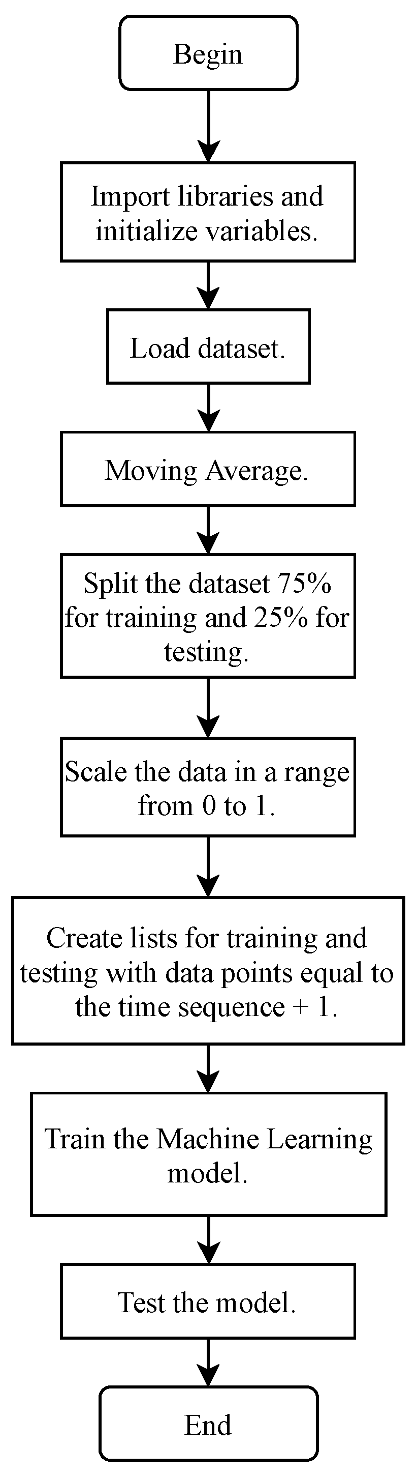
2.1. Data Preprocessing

It is common to find missing values in databases represented by zeros, probably due to sensor failures. The article [25] impute the missing data points using the historical average value, and [20] reports substituting these values with the mean of the entire column containing the missing value. Although these substituted data are not realistic values, the researchers determined that they are better than no data. However, when performing the predictions, this procedure generates spikes in the real values, increasing the error because, on some occasions, the trend shows that the zero values were real. These spikes are highlighted in red rectangles as shown in Figure 1a; this is why a moving average is applied using the 12 previous readings. Figure 1b shows how abrupt changes caused by the general average are avoided. Next, the database is split into 75% of the data (42 days) for training and 25% (14 days) for testing.
The data are scaled in a range from 0 to 1, following the standard normal distribution using MinMaxScaler from scikit-learn library [33]. For this experiment, the previous hour’s traffic flow is used, which is a time sequence of 12 data points, to predict the traffic flow coming in the next five minutes. To do this, lists are created grouped into 13 readings; these lists are used for training and testing purposes. The generated lists are then converted into arrays and the training sequence is shuffled. Once this is done, the last column of the arrays is taken as the output ‘Y’, and the remaining columns as the inputs ‘X’.

2.2. Recurrent Neural Networks

2.2.1. RNNs Design

Two recurrent neural networks are designed: GRU and LSTM. Keras library [34] is used to create the models. The architecture is the same for both as shown in Figure 2 and explained below: The input layer with shape equal to the number of time steps per the number of lanes. Then two recurrent layers with 64 neurons, 20% dropout, and finally, an output layer with neurons equal to the number of lanes and sigmoid activation function.

2.2.2. RNNs Training

In the compilation of the model, mean squared error (MSE) is used as loss function, and the optimizer is RMSprop from Keras library [34] with default parameters and mean absolute error (MAE) is the metric function. For training, a batch size of 128 and 50 epochs are used, five percent of the training data is used for validation. The experiments are performed in Google Colaboratory [35] along with Weights & Biases [36] for tracking them. Figure 3 shows the training performance of the two architectures, where the loss and evaluation metrics in training and validation can be observed.

2.3. Machine Learning Methods
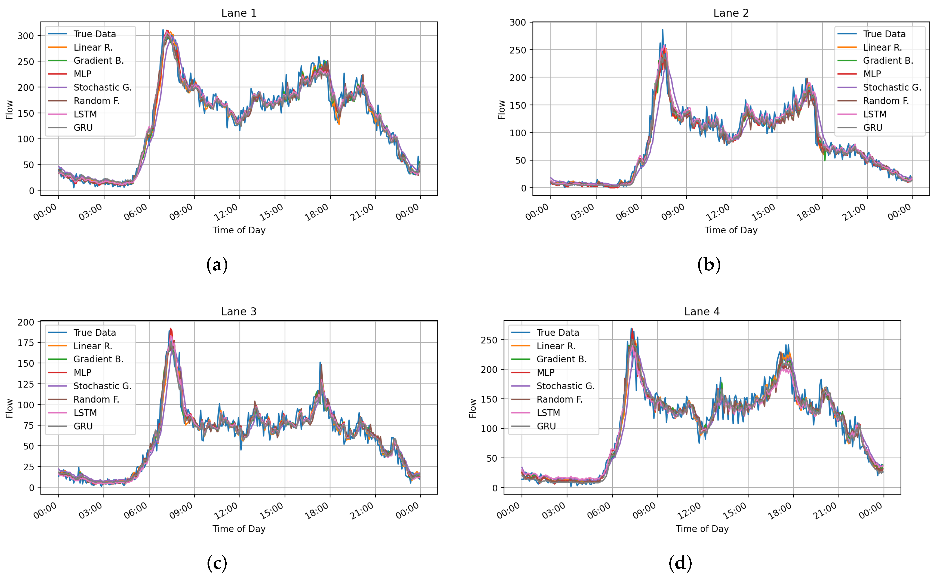
Five regression models from the scikit-learn library [33] in Python are used: Linear Regression, Gradient Boosting Regressor, MultiLayer Perceptron Regressor, Stochastic Gradient Descendent Regressor and Random Forest Regressor, all of them with default parameters and a random state equal to zero for the reproducibility of the experiment. A reshape of ‘X’ for both training and testing is made because these models require a 2D array instead of the 3D used in the RNN’s; after that, the models are fed with the training split. The methodology summary presented in the form of a flowchart is shown in Figure 4.

3. Results

To evaluate the performance of ML and DL algorithms, first, an inverse scaler was applied to the ’y’ test. Then we relied on the metrics of the scikit-learn library [33], the mean absolute error (MAE) [21,37], root mean square error (RMSE) [7,29], mean absolute percent error (MAPE) [14,15], R-squared ( R 2 ) [3,9] and explained variance (EV) are used. They are defined as:
MAE ( y , y ^ ) = 1 n i = 0 n 1 y i y ^ i
MAPE ( y , y ^ ) = 100 % n i = 0 n 1 y i y ^ i y i
RMSE ( y , y ^ ) = 1 n i = 0 n 1 y i y ^ i 2 1 2
R 2 ( y , y ^ ) = 1 i = 1 n y i y ^ i 2 i = 1 n y i y ¯ 2
explained _ variance ( y , y ^ ) = 1 V a r y y ^ V a r y
where n is the number of samples, y is the observed traffic flow, y ^ is the predicted traffic flow and y ¯ is the mean.
MAE and RMSE measure absolute prediction errors, and MAPE measures relative prediction errors. Smaller numbers indicate higher prediction performance for these three metrics [37]. The values of R 2 and EV range from zero to one, and the closer to the value of one the better the regression model fits.
Table 1 lists the performance metrics of each ML and DL models, Multilayer Perceptron and Gradient Boosting obtained R-Squared and Explained Variance above 0.93, MAE of 10.8, MAPE of 21% and RMSE of 15.4. In contrast, Random Forest had an R-squared and Explained Variance slightly below 0.93, MAE of 10.88, MAPE of 21% and RMSE of 15.5. While GRU and LSTM obtained R-Squared and Explained Variance near 0.92, MAE of 10.88, MAPE of 22% and RMSE of 15.6, Linear Regression R-Squared and Explained Variance were 0.926, MAE of 11.2, MAPE of 24% and RMSE of 15.85; finally, Stochastic Gradient had R-Squared and Explained Variance of 0.9, MAE of 12.8, MAPE of 29% and RMSE of 18.
For the results shown, RNNs are iteratively trained ten times, and the average of each metric is calculated; in the case of the ML models (scikit-learn), the random state allows us to have the same results each time.
Additionally, robustness testing was performed using a different dataset [25] than the one initially used for training and validation. These new data are collected from the PeMS dataset, which has over 15,000 sensors deployed throughout the state of California, specifically the fourth district, which lies in the Bay Area, Alameda, Oakland of the U.S. For robustness, R 2 and EV score are good parameters because these metrics are dimensionless, work for different datasets of different scales and are normalized. The metrics obtained with the external dataset are listed in Table 2. Comparing the results of R 2 and EV score listed in Table 1 and Table 2, it can be observed that in both cases R 2 and EV score are between the values of 0.9 and 0.95. Therefore, since R 2 and EV remain within the same range regardless of the dataset, we can confirm that the proposed models are robust for traffic flow prediction.
On the other hand, to analyze the cost-benefit of the implementation of the models, the average training time was obtained for each one of them, the experiments were carried out in the Google Colaboratory [35] execution environment, and also [36] was used to keep track of the times. Figure 5 depicts the training time of the seven ML models tested in this study. It is important to note that scikit learn models train takes less time than designed RNN’s. LSTM and GRU models are the ones with the longer training time 321 and 250 seconds, among the scikit learn models Random Forest, Gradient Boosting, Linear Regression, Stochastic Gradient and MLP-NN 46, 28, 20, 20 and 18 seconds being MLP-NN the fastest and it is the model that also has better performance metrics, as shown in Table 1.
Predictions performed over the test split for one day in the four lanes are shown in Figure 6 and for an entire week are plotted in Figure 7.

4. Proposed Usage Scenario

These models can be used in a smart traffic light controller, fed by traffic sensors that count the number of vehicles passing through a lane every certain period; with these readings, a database similar to the one used in this paper can be created. Once the database is generated, the ML model can be trained for each intersection. Then the traffic flow for the next period can be predicted by using a given number of past readings.
Once the prediction is made, it will allow better programming of the times of each state, either manually by an operator or automatically using an algorithm to calculate the optimal times of the traffic light states. The whole process can be carried out by wirelessly communicating the traffic light with a central station or at the controller itself. Figure 8a shows a block diagram of the main elements of the proposed system and Figure 8b its representation in a real-world scenario.

5. Conclusions

In this paper, we proposed several ML and DL models for the traffic flow prediction at an intersection of vehicular traffic, thus laying the groundwork for adaptive traffic control. Two public datasets were used to train, validate and test the proposed models. Experimental results showed that Multilayer Perceptron Regressor has better performance and takes less processing time to train (18 s). Gradient Boosting Regressor has a similar performance but takes more processing time (28 s). Both RNNs and Random Forest Regressor have a similar score. However, RNNs are slow to train (between 250 and 321 s). Finally, Linear Regression and Stochastic Gradient Regressor have good processing time (20 s) but are the worst performance between these models. All ML and DL models achieved an explained variance score (EV Score) and R-squared ( R 2 ) greater than 0.90, MAE near to 10; the RMSE is near 15 and the MAPE is between 20 and 30 percent. Actually, the performance of these seven algorithms does not differ significantly. In conclusion, the results were satisfactory for predicting traffic flow in the four lanes of an intersection, demonstrating the feasibility of being implemented on smart traffic light controllers.

Author Contributions

Conceptualization, O.R.L.-B. and E.I.-G.; Data curation, D.L.-M. and C.H.-M.; Formal analysis, E.T.-C. and D.L.-M.; Funding acquisition, O.R.L.-B.; Investigation, A.N.-E. and E.T.-C.; Methodology, A.N.-E.; Project administration, O.R.L.-B.; Resources, O.R.L.-B. and D.L.-M.; Software, A.N.-E. and E.I.-G.; Supervision, O.R.L.-B. and E.I.-G.; Validation, E.E.G.-G., E.T.-C. and D.L.-M.; Visualization, E.E.G.-G. and C.H.-M.; Writing-original draft, A.N.-E.; Writing-review and editing, E.T.-C. and E.I.-G. All authors have read and agreed to the published version of the manuscript.

Funding

This research was funded by the Universidad Autonoma de Baja California (UABC) through the 22th internal call with grant number 679.

Institutional Review Board Statement

Not applicable.

Informed Consent Statement

Not applicable.

Data Availability Statement

Data are available at: https://zenodo.org/record/3653880#.YZbTcE6ZND9 (First dataset, accessed on 20 December 2021), and https://doi.org/10.1109/YAC.2016.7804912 (Second dataset, accessed on 20 December 2021)).

Acknowledgments

The authors would like to thank INAOE and UDG for accepting researcher Everardo Inzunza-González to carry out his sabbatical stay. Thanks are given to PRODEP (Professional Development Program for Professors) for supporting the academic groups to increase their degree of consolidation. The authors are thankful to the reviewers for their comments and suggestions to improve the quality of the manuscript.

Conflicts of Interest

The authors declare no conflict of interest.

References

  1. Chen, C.; Liu, B.; Wan, S.; Qiao, P.; Pei, Q. An Edge Traffic Flow Detection Scheme Based on Deep Learning in an Intelligent Transportation System. IEEE Trans. Intell. Transp. Syst. 2021, 22, 1840–1852. [Google Scholar] [CrossRef]
  2. Ahmed, M.; Masood, S.; Ahmad, M.; El-Latif, A.A.A. Intelligent Driver Drowsiness Detection for Traffic Safety Based on Multi CNN Deep Model and Facial Subsampling. IEEE Trans. Intell. Transp. Syst. 2021, 1–10. [Google Scholar] [CrossRef]
  3. Boukerche, A.; Wang, J. A performance modeling and analysis of a novel vehicular traffic flow prediction system using a hybrid machine learning-based model. Ad. Hoc. Netw. 2020, 106, 102224. [Google Scholar] [CrossRef]
  4. Meena, G.; Sharma, D.; Mahrishi, M. Traffic Prediction for Intelligent Transportation System using Machine Learning. In Proceedings of the 2020 3rd International Conference on Emerging Technologies in Computer Engineering: Machine Learning and Internet of Things (ICETCE), Jaipur, India, 7–8 February 2020; pp. 145–148. [Google Scholar] [CrossRef]
  5. Yuan, H.; Li, G. A Survey of Traffic Prediction: From Spatio-Temporal Data to Intelligent Transportation. Data Sci. Eng. 2021, 6, 63–85. [Google Scholar] [CrossRef]
  6. Jingyao, W.; Manas, R.P.; Nallappan, G. Machine learning-based human-robot interaction in ITS. Inf. Process. Manag. 2022, 59, 102750. [Google Scholar] [CrossRef]
  7. Li, Y.; Shahabi, C. A brief overview of machine learning methods for short-term traffic forecasting and future directions. Sigspatial Spec. 2018, 10, 3–9. [Google Scholar] [CrossRef]
  8. Boukerche, A.; Wang, J. Machine Learning-based traffic prediction models for Intelligent Transportation Systems. Comput. Netw. 2020, 181, 107530. [Google Scholar] [CrossRef]
  9. Boukerche, A.; Tao, Y.; Sun, P. Artificial intelligence-based vehicular traffic flow prediction methods for supporting intelligent transportation systems. Comput. Netw. 2020, 182, 107484. [Google Scholar] [CrossRef]
  10. Ahsan, M.M.; Mahmud, M.A.P.; Saha, P.K.; Gupta, K.D.; Siddique, Z. Effect of Data Scaling Methods on Machine Learning Algorithms and Model Performance. Technologies 2021, 9, 52. [Google Scholar] [CrossRef]
  11. George, S.; Santra, A.K. Traffic Prediction Using Multifaceted Techniques: A Survey. Wirel. Pers. Commun. 2020, 115, 1047–1106. [Google Scholar] [CrossRef]
  12. Alam, I.; Farid, D.M.; Rossetti, R.J.F. The Prediction of Traffic Flow with Regression Analysis. In Emerging Technologies in Data Mining and Information Security; Abraham, A., Dutta, P., Mandal, J.K., Bhattacharya, A., Dutta, S., Eds.; Springer: Singapore, 2019; pp. 661–671. [Google Scholar]
  13. Li, J.; Boonaert, J.; Doniec, A.; Lozenguez, G. Multi-models machine learning methods for traffic flow estimation from Floating Car Data. Transp. Res. Part C: Emerg. Technol. 2021, 132, 103389. [Google Scholar] [CrossRef]
  14. Haghighat, A.K.; Ravichandra-Mouli, V.; Chakraborty, P.; Esfandiari, Y.; Arabi, S.; Sharma, A. Applications of Deep Learning in Intelligent Transportation Systems. J. Big Data Anal. Transp. 2020, 2, 115–145. [Google Scholar] [CrossRef]
  15. Ferreira, Y.; Frank, L.; Julio, E.; Henrique, F.; Dembogurski, B.; Silva, E. Applying a Multilayer Perceptron for Traffic Flow Prediction to Empower a Smart Ecosystem. In Computational Science and Its Applications; Springer: Cham, Switzerland, 2019; pp. 633–648. [Google Scholar] [CrossRef]
  16. Hosseini, S.H.; Moshiri, B.; Rahimi-Kian, A.; Araabi, B.N. Traffic flow prediction using mi algorithm and considering noisy and data loss conditions: An application to minnesota traffic flow prediction. Promet Traffic Traffico 2014, 26, 393–403. [Google Scholar] [CrossRef]
  17. Jiang, C.Y.; Hu, X.M.; Chen, W.N. An Urban Traffic Signal Control System Based on Traffic Flow Prediction. In Proceedings of the 2021 13th International Conference on Advanced Computational Intelligence (ICACI), Wanzhou, China, 14–16 May 2021; pp. 259–265. [Google Scholar] [CrossRef]
  18. Chen, Y.R.; Chen, K.P.; Hsiung, P.A. Dynamic traffic light optimization and control system using model-predictive control method. In Proceedings of the IEEE Conference on Intelligent Transportation Systems (ITSC), Rio de Janeiro, Brazil, 1–4 November 2016; pp. 2366–2371. [Google Scholar] [CrossRef]
  19. Wang, R. Optimal method of intelligent traffic signal light timing based on genetic neural network. Adv. Transp. Stud. 2021, 1, 3–12. [Google Scholar] [CrossRef]
  20. Lawe, S.; Wang, R. Optimization of Traffic Signals Using Deep Learning Neural Networks BT—AI 2016: Advances in Artificial Intelligence. In AI 2016: Advances in Artificial Intelligence; Kang, B.H., Bai, Q., Eds.; Springer: Cham, Switzerland, 2016; pp. 403–415. [Google Scholar] [CrossRef]
  21. Chen, Q.; Song, Y.; Zhao, J. Short-term traffic flow prediction based on improved wavelet neural network. Neural Comput. Appl. 2021, 33, 8181–8190. [Google Scholar] [CrossRef]
  22. Gadze, J.D.; Bamfo-Asante, A.A.; Agyemang, J.O.; Nunoo-Mensah, H.; Opare, K.A.B. An Investigation into the Application of Deep Learning in the Detection and Mitigation of DDOS Attack on SDN Controllers. Technologies 2021, 9, 14. [Google Scholar] [CrossRef]
  23. Zhang, Y.; Xin, D.R. Short-term traffic flow prediction model based on deep learning regression algorithm. Int. J. Comput. Sci. Math. 2021, 14, 155–166. [Google Scholar] [CrossRef]
  24. Lei, H.; Yi-Shao, H. Short-term traffic flow prediction of road network based on deep learning. IET Intell. Transp. Syst. 2020, 14, 495–503. [Google Scholar] [CrossRef]
  25. Fu, R.; Zhang, Z.; Li, L. Using LSTM and GRU neural network methods for traffic flow prediction. In Proceedings of the 2016 31st Youth Academic Annual Conference of Chinese Association of Automation, YAC 2016, Wuhan, China, 11–13 November 2016; pp. 324–328. [Google Scholar] [CrossRef]
  26. Hussain, B.; Afzal, M.K.; Ahmad, S.; Mostafa, A.M. Intelligent Traffic Flow Prediction Using Optimized GRU Model. IEEE Access 2021, 9, 100736–100746. [Google Scholar] [CrossRef]
  27. Lv, Y.; Duan, Y.; Kang, W.; Li, Z.; Wang, F.Y. Traffic Flow Prediction with Big Data: A Deep Learning Approach. IEEE Trans. Intell. Transp. Syst. 2015, 16, 865–873. [Google Scholar] [CrossRef]
  28. Cui, Z.; Huang, B.; Dou, H.; Tan, G.; Zheng, S.; Zhou, T. GSA-ELM: A hybrid learning model for short-term traffic flow forecasting. IET Intell. Trans. Syst. 2021, 16, 1–12. [Google Scholar] [CrossRef]
  29. Luo, C.; Huang, C.; Cao, J.; Lu, J.; Huang, W.; Guo, J.; Wei, Y. Short-Term Traffic Flow Prediction Based on Least Square Support Vector Machine with Hybrid Optimization Algorithm. Neural Process. Lett. 2019, 50, 2305–2322. [Google Scholar] [CrossRef]
  30. Axenie, C.; Bortoli, S. Road Traffic Prediction Dataset. 2020. Available online: https://zenodo.org/record/3653880#.YdupBWhBxPY (accessed on 20 December 2021).
  31. Hou, Y.; Chen, J.; Wen, S. The effect of the dataset on evaluating urban traffic prediction. Alex. Eng. J. 2021, 60, 597–613. [Google Scholar] [CrossRef]
  32. Chen, C.; Wang, Y.; Li, L.; Hu, J.; Zhang, Z. The retrieval of intra-day trend and its influence on traffic prediction. Transp. Res. Part C Emerg. Technol. 2012, 22, 103–118. [Google Scholar] [CrossRef]
  33. Pedregosa, F.; Varoquaux, G.; Gramfort, A.; Michel, V.; Thirion, B.; Grisel, O.; Blondel, M.; Prettenhofer, P.; Weiss, R.; Dubourg, V.; et al. Scikit-Learn: Machine Learning in Python. 2011. Available online: scikit-learn.org (accessed on 20 December 2021).
  34. Chollet, F. Keras. 2015. Available online: keras.io (accessed on 20 December 2021).
  35. Bisong, E. Google Colaboratory BT—Building Machine Learning and Deep Learning Models on Google Cloud Platform: A Comprehensive Guide for Beginners. 2019. Available online: https://link.springer.com/chapter/10.1007/978-1-4842-4470-8_7 (accessed on 20 December 2021).
  36. Biewald, L. Experiment Tracking with Weights and Biases. 2020. Available online: wandb.com (accessed on 20 December 2021).
  37. Cai, L.; Janowicz, K.; Mai, G.; Yan, B.; Zhu, R. Traffic transformer: Capturing the continuity and periodicity of time series for traffic forecasting. Trans. GIS 2020, 24, 736–755. [Google Scholar] [CrossRef]
Figure 1. Differences between the substitution of zeros applying a general average and a moving average. (a) General Average; (b) Moving Average.
Technologies 10 00005 g001
Figure 2. Architecture of the recurrent neural networks. (a) LSTM-NN; (b) GRU-NN.
Technologies 10 00005 g002
Figure 3. Training performance of both neural networks. (a) LSTM NN; (b) GRU NN.
Technologies 10 00005 g003
Figure 4. Flowchart of proposed method.
Technologies 10 00005 g004
Figure 5. Comparison of training times.
Technologies 10 00005 g005
Figure 6. Comparison of traffic flow prediction models for one test day. (a) Traffic flow prediction of lane 1; (b) Traffic flow prediction lane 2; (c) Traffic flow prediction lane 3; (d) Traffic flow prediction lane 4.
Technologies 10 00005 g006
Figure 7. Comparison of traffic flow prediction models over an entire week. (a) Traffic flow prediction of lane 1; (b) Traffic flow prediction lane 2; (c) Traffic flow prediction lane 3; (d) Traffic flow prediction lane 4.
Technologies 10 00005 g007
Figure 8. Proposed usage. (a) Block diagram; (b) Representation in real-world scenario.
Technologies 10 00005 g008
Table 1. Comparison of performance metrics using the first dataset [30].
ML/DL ModelMAEMAPERMSE R 2 EV Score
MLP-NN10.828121.1593%15.42020.93040.9307
Gradient Boosting10.850821.9493%15.41210.93050.9306
Random Forest10.882721.8392%15.54810.92960.9297
GRU10.884322.8492%15.61910.92780.9295
LSTM10.880622.3244%15.67710.92670.9287
Linear Regression11.201024.3238%15.85450.92630.9264
Stochastic Gradient12.823029.0075%18.37270.90030.9004
Table 2. Performance metrics using the second dataset (PeMS) [25].
ML/DL ModelMAEMAPERMSE R 2 EV Score
MLP-NN7.242718.21769.80960.93930.9395
Gradient Boosting7.1215117.62249.66480.9410.941
Random Forest7.0504617.37889.57990.94210.9421
GRU7.6426618.530710.24060.93380.9381
LSTM7.3285219.09239.88160.93840.9388
Linear Regression7.5169320.382210.19140.93440.9344
Stochastic Gradient8.3924323.744311.31990.91910.9194
Publisher’s Note: MDPI stays neutral with regard to jurisdictional claims in published maps and institutional affiliations.

