1. Introduction
The current financial context at the European level is one influenced by inflation and a higher need for financing based on the rising cost of living, induced by the vulnerabilities of multiple crises triggered by pandemics and geopolitical conflict.
On 8 July 2021, the European Central Bank (ECB) published its new monetary policy strategy with the primary objective of maintaining price stability in the euro area (
European Central Bank Strategy 2023). The ECB’s previous strategies have focused on closing the gaps in the effects on inflation and price stability at the European level.
Structural developments in the euro area between 2003 and 2021 have resulted in a reduction in the equilibrium interest rate and economic growth driven by demographic dynamics and an increased demand for liquid assets.
On top of these ambitious targets, the effects of uncertainties during the economic crisis (2008–2012) have manifested themselves, posing real challenges to monetary policy objectives and the maintenance of conventional policies in the face of inflationary shocks. Fluctuating inflation margins in times of crisis have demonstrated the need to implement additional policy instruments.
Another significant moment in the euro area was marked by the sovereign debt crisis of Greece (
Bank of Greece Monetary Policy 2023) and Spain (
Banco de Espana Monetary Policy 2023), which triggered the need for assistance to maintain the stability of these countries and implement monetary policy measures. Another destabilizing event was the outbreak of the COVID-19 pandemic in Europe, when the European community faced economic slowdown and rising unemployment.
In this extremely challenging financial equation, globalization and digitalization, which have changed the traditional structure of European economies and labor markets, can be mentioned as disruptive factors. Included in the picture of challenges are reforms to support changes in the institutional architecture of the euro area, which has undergone significant transformations and changes during this period.
Romania joined the EU in 2007 and is currently a point of vulnerability as the significant economic progress it has made in the post-accession period has not led to institutional integration into the European architecture, with Romania and Bulgaria still sticking to their national currencies and failing to switch to the euro as other countries such as Croatia, which joined in 2013, have managed to (
European Commision Economy and Finance 2023). In this context, our approach based on the identification of a dynamic structured model of Romanian monetary policy in conditions of uncertainty acquires particular importance and topicality both in relation to the strategic objectives of the EU and in relation to the reduction in economic and financial disparities between Member States as a basis for sustainable European development.
We consider that Romania is representative of all non-euro member states that are not able to achieve the adhering criteria for the euro area (
European Commission ERM II 2020). The economic growth in Romania and the characteristics of the monetary market support this idea.
Monetary policy elements in Romania were adjusted on the basis of volatility indicators for the annual inflation rate, which for August 2022 increased by 0.3% from the previous month’s level (from 13% to 13.3%). On the other hand, the influence of rising inflation through the consumer index and trade shocks was felt at the European level in the euro area, with the inflation rate reaching 10% in September 2022. The economic environment was based on a reduction in the growth rate from 5.1% in Q1 to 2.1% in Q2, with a moderate increase in the aggregate demand surplus expected over the forecast period (
BNR 2022).
The real interest rate that is in equilibrium and consistent with price stability is known as the natural rate of interest, or simply the “natural rate”. Romania has experienced a steady increase in inflation over the past few years, which has led to a higher natural rate of interest (
BNR 2022). As the central bank attempted to control inflation, it raised interest rates to align them with the natural rate. This had implications for borrowing costs, investment decisions, and overall economic growth in Romania. According to the literature, higher interest rates can discourage borrowing and lead to increased borrowing costs for businesses and individuals (
Drazen 2000). This can potentially slow down investment decisions and reduce consumer spending, which can negatively impact economic growth. Additionally, higher interest rates can attract foreign investors seeking higher returns, which can strengthen the country’s currency and potentially negatively affect export competitiveness. Therefore, it is important for the central bank to carefully assess the implications of adjusting interest rates in order to maintain a balance between controlling inflation and promoting sustainable economic growth. By carefully assessing the implications of adjusting interest rates, the central bank can ensure that inflation remains under control while also fostering sustainable economic growth. Implementing interest rate adjustments without careful consideration could lead to unintended consequences such as reduced consumer spending and weakened export competitiveness. Striking a balance between these factors is essential for maintaining a healthy economy and avoiding any potential negative impacts on economic growth. From our point of view, reaching an equilibrium on this issue requires a lot of information, which is difficult to correlate because of the complexity of the area under development research in the field.
Other elements of the influence of the uncertain environment marked by the geopolitical conflict, the energy crisis and the health crisis are the decrease in the contribution of private consumption to the GDP, which is mainly due to changes in inventories, the decrease in the dynamics of retail trade and services provided to the population, the contraction of industrial production and the volume of new orders, and the slight shrinkage of the employment (
BNR 2022). In the same trend, the dynamics of credit to the private sector decreased from 17.5% in June 2022 to 15.9% in August.
The adoption of the euro could have potentially stabilized Romania’s inflation rate by providing a fixed exchange rate and reducing the uncertainty associated with fluctuating currency values. This stability could have helped maintain price stability, preventing the rapid price increases that often accompany economic turmoil. The Euro’s adoption could have made Romania more attractive to foreign investors and facilitated trade with other Eurozone countries, potentially boosting its competitiveness in international markets. Additionally, being part of a larger economic bloc may have given Romania a stronger negotiating position in trade agreements, allowing for more favorable terms. However, it is worth considering that joining the Eurozone could also have led to increased competition from other member states, potentially challenging Romania’s market share. With the euro being a stable and widely accepted currency, Romania’s adoption of it could have instilled greater trust and security among foreign investors, leading to increased FDI inflows. On the other hand, if the economic turmoil in Romania was perceived as a risk, some investors might have chosen to withdraw their investments, resulting in FDI outflows. Therefore, understanding the relationship between the euro and FDI flows is crucial in assessing the impact of currency adoption on Romania’s macroeconomy. The adoption of the euro would have likely led to a more disciplined approach to government spending, as Romania would have had to adhere to the fiscal rules set by the European Union. This could have potentially helped in reducing budget deficits and controlling inflation. Secondly, taxation policies may have also been affected, with the euro adoption possibly leading to changes in tax rates and structures to align with the EU’s tax policies. Lastly, the adoption of the euro would have also impacted Romania’s public debt, as it would have been denominated in euros instead of the national currency. This could have resulted in increased borrowing costs and stricter debt management strategies to maintain fiscal stability. All the more so since in April 2023, the European Commission unveiled two comprehensive thematic reports addressing the topics of competitiveness and external balances. These reports also encompass an analysis of the situation in Romania. The data indicate that Romania’s external position has experienced a deterioration since 2015. At the conclusion of 2022, the current account deficit exhibited a notable increase, rising from 7.2% of GDP in 2021 to 9.3% of GDP. This surge in deficit is in close proximity to the 5% recorded in 2020, mostly due to trade and primary income balances experiencing an additional decrease toward a deficit (
European Commission In-Depth Review for Romania 2023).
These aspects motivate the scientific approach to conceptualize a dynamic structured model of Romanian monetary policy under uncertainty based on the following research objectives:
O1: The identification of models for monetary policy analysis under uncertainty in the literature;
O2: A literature-based dissemination of working hypotheses;
O3: The conceptualization, testing and implementation of the dynamic structured monetary policy model;
O4: A dissemination of the results of the model;
O5: The making of proposals to adjust monetary policies under uncertainty.
The present research continues with the study of the literature; we will perform a bibliometric analysis of current publications in the field of monetary policy, highlighting clusters of research interests adjacent to the field (fiscal policy, inflation, financial stability, monetary policy instruments, liquidity, etc.), followed by an analysis of the methodology, using which we will perform the logical scheme of the study and mathematically conceptualize the economic model, following which the results and discussions will practically disseminate the observations drawn from modeling, and the conclusions will capture the general elements of the study.
2. Literature Review
In the literature, monetary policies are a topic of real interest, both because of their direct relationship with monetary policy indicators and because of their influence on the financial economies of countries with implications for economic entities.
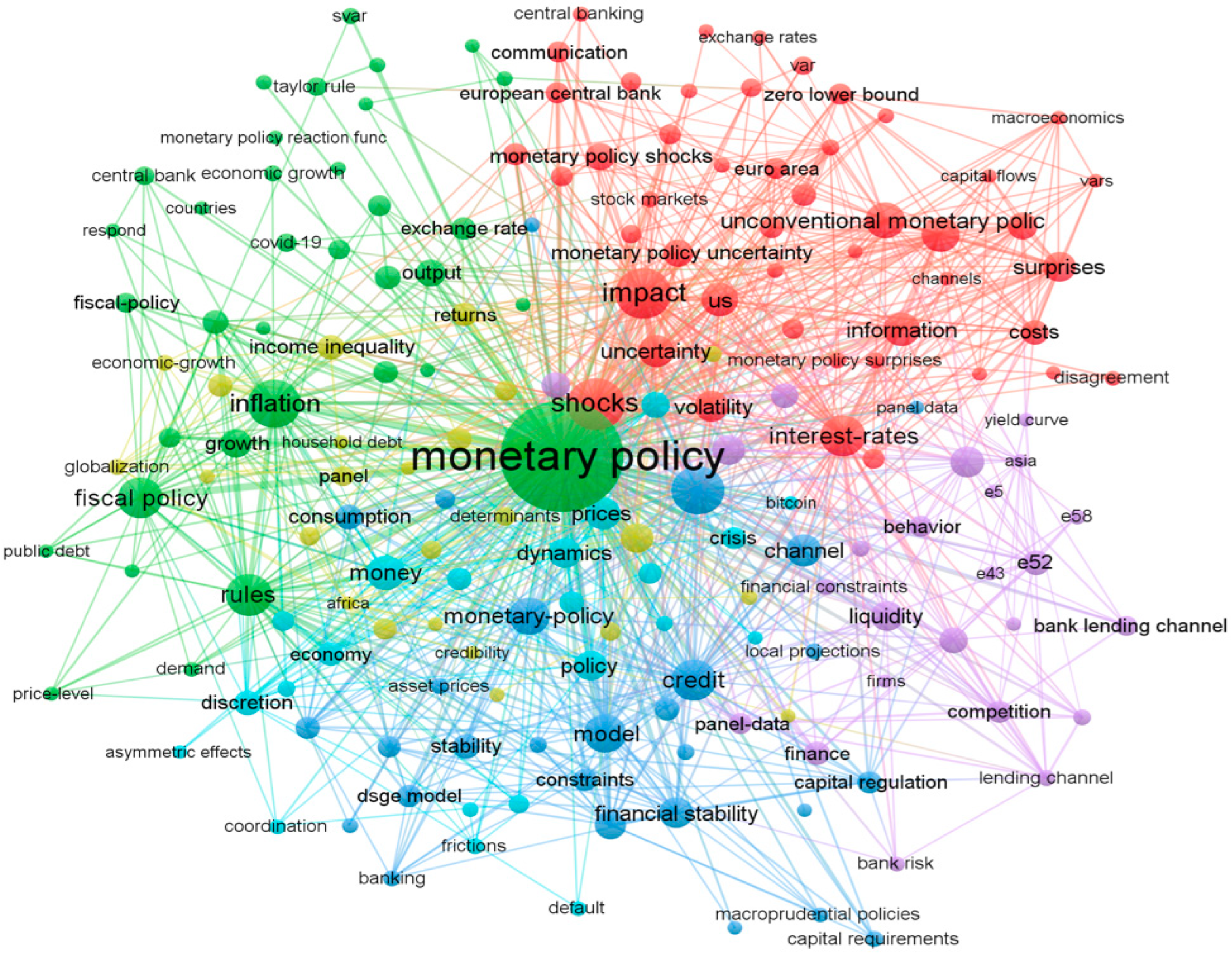
From the analysis of Web of Science publications, we observed that of the 6988 articles published in the period 2020–2022 (
Figure 1), citations were found at the level of 2.71 papers per article with a corresponding Hirsch index of 43 points, which shows the interest of researchers in financial markets under the impact of risk factors and monetary policies, the role of information shocks in the economy, the impact of monetary policies in pandemics on share prices, the role of central banks, the impact of financial development on some elements of macroeconomic policy, global effects of uncertainty-induced pandemics, monetary policy under the impact of uncertainty, etc. The bibliometrics analysis data were extracted from the Web of Science platform and then integrated and processed in VOSviewer.
The paradigm of this discussion is the direction of causality in the monetary aggregates. Is money endogenous or is it exogenous to the overall system? This debate has been a topic of discussion among economists for many years. One point of view argues that money is endogenous, meaning that its supply is determined by the demand for credit and the actions of banks. According to this view, changes in the overall system, such as changes in interest rates or economic conditions, will ultimately impact the money supply.
A second point of view argues that money is controlled by the central bank and is thus exogenous to the system. As a result, changes in the money supply are a deliberate policy tool used by central banks to influence the economy. The direction of causality in monetary aggregates remains a complex and ongoing area of research in economics.
Some of the greatest economists of the world were focused on this issue.
Friedman (
1990), for example, pointed out that the scholarly discourse surrounding the aims and instruments employed in monetary policy is intrinsically intertwined with the dichotomy between activist and nonresponsive approaches. Nonresponsiveness is a straightforward strategy that entails dealing with particular problems or making the necessary adjustments, whereas activism entails acting in response to the initial conditions or signs of disruptions while following various feedback rules. However, it is worth noting that the nonresponsive rules that have garnered significant attention in the past primarily pertain to endogenous variables such as money rather than exogenous variables that can be directly controlled by the central bank (e.g., nonborrowed reserves). Consequently, the fundamental inquiry revolves around determining the categories of phenomena that warrant a response and those that do not, rather than debating whether or not to respond altogether. The restricted relevance of activist critique policy, which argues that deviating from the no-response or base position generally leads to uncertainty, points out a significant lack of knowledge; such uncertainty may even escalate and result in an increase in the variability of the policy objective rather than its reduction.
A.W. Phillips (
1958) analyzed the relationship between inflation and unemployment in an economy. Phillips suggests that there is an inverse relationship between the two variables: when unemployment is low, inflation tends to be high, and vice versa. This concept has been widely debated and studied by economists, as it helps in understanding the dynamics of an economy and formulating monetary policies. According to the author, in situations where demand exceeds supply, the price of a product or service increases, with the increase being proportional to the excess demand. Conversely, when demand is lower than supply, the price decreases, with the decline being more significant when there is a higher disparity between demand and supply. This principle could influence the rate at which money wage rates, representing labor services’ prices, change over time. In periods of high labor demand and low unemployment, wage rates may increase rapidly as companies attract qualified labor from other firms and industries. However, during periods of low labor demand and high unemployment, wages may decline gradually. The correlation between unemployment and pay rate change is expected to be non-linear, with a potential correlation between the rate of change in money wage rates and the rate of change in labor demand, which affects unemployment levels. In a period of increased economic activity with rising labor demand and declining unemployment, employers engage in more competitive bidding for labor services. Conversely, in a year with a decline in business activity and decreased labor demand, employers are less willing to provide wage increases, leaving workers in a disadvantageous position to negotiate for wage increases. The rate of change of retail prices also influences the rate of change of money wage rates, as cost of living adjustments in wage rates can exert a minimal or negligible influence on the rate of change in money pay rates.
In a piece of interesting research,
Laidler (
2023) considered that contemporary macroeconomics assumes a perpetual equilibrium when analyzing the economy, but two theoretical frameworks, monetarism and the Wicksell connections (
Wicksell 1907), argue that information acquisition and coordination by economic agents should be primary concerns. The first approach addresses concerns related to monetary exchange, while the second focuses on inter-temporal issues. Both approaches, particularly within the framework of the dynamic stochastic general equilibrium (DSGE),
Schumpeter and Keynes (
1936) analysis, consider the coordination of activities among individual economic agents as a fundamental issue for any economy and economists analyzing it. Both approaches also see monetary exchange and financial markets as essential components in adaptation and resilience. The Wicksell connection, on the other hand, emphasizes the challenges associated with coordinating economic activity over time. The existing divide between the two traditions has not been resolved, but it is narrower compared to the significant disparity between them and the mainstream DSGE. The mainstream approach assumes that coordination issues are resolved via assumption before conducting in-depth analysis.
John B. Taylor’s 1993 proposition (
Taylor 1993) outlined US monetary policy as an interest rate feedback rule, where the Federal Reserve adjusts the nominal interest rate in response to inflation and output deviations. The central bank aims to achieve economic stability and maintain manageable inflation levels. According to
Woodford (
2001), Taylor’s proposal has significantly influenced monetary policy discourse. The question is whether or not this rule can establish an equilibrium price level without a target route for monetary aggregates. Critics argue that interest rate rules can lead to the indeterminacy of the equilibrium price level under rational expectations, but this is dependent on the presence of an external trajectory for the short-term nominal interest rate. Determinacy can be achieved through feedback from an endogenous state variable, such as the price level. Many basic optimization models suggest that the Taylor rule includes determinacy feedback, as the operating goal for the funds rate relies on recent inflation and output gap indicators.
From Cagan’s point of view (
Cagan and Gandolfi 1969), the time lag between the implementation of monetary policies and their impact on output and employment is a contentious issue in monetary policy. According to the authors, classical research suggests a time delay of two to six quarters or more, with some arguing for a reduced duration due to potential revenue fluctuations. In the context of the money supply, the conduct of monetary policy is entirely encapsulated by the dynamics of the money supply, and the potential time delay between policy measures and their impact is disregarded. One enduring premise in monetary theory is that an expansion in the money supply leads to a decrease in interest rates. This phenomenon may be attributed to the unintended consequences of the growth of the financial system. This effect signifies the functional relationship between money demand and interest rates. The impact of a monetary adjustment on interest rates is transitory and does not endure in the long term. Greater balances and lower interest rates stimulate increased expenditure on consumer and producer capital goods, which in turn leads to an increase in income and counteracts the initial impact of the monetary increase on interest rates. According to the authors, in full employment scenarios, an increase in prices results in a decrease in the actual worth of money balances, raising interest rates. If growth begins with underutilized labor resources, a portion of the rise in income will manifest as an increase in purchasing power, adjusted for inflation. An increase in either nominal or real income generally results in an upward movement in interest rates, although the magnitude of this effect may differ.
An interesting scientific approach realized by
Bassetto and Sargent (
2020) examines the interplay between monetary and fiscal policies and their impact on equilibrium price levels and interest rates. It critically assesses various theories pertaining to optimal anticipated inflation, optimal unanticipated inflation, and the conditions necessary to establish a nominal anchor, ensuring a singular path for price levels. In this analysis, we examine the distinction between incomplete theories and complete theories. The former relies on budget-viable sequences of government-issued bonds and money as inputs, while the latter utilizes bond and money strategies expressed as sequences of functions that map time t history into time t government actions. According to the authors’ theoretical perspective, the delineation of power dynamics between a treasury and a central bank can be characterized by ambiguity, opacity, and vulnerability.
Larry
Summers (
1991) argued that in order to achieve long-term price stability, monetary policy should be based on a flexible inflation target. He emphasized the importance of allowing some level of inflation, as a very low inflation rate can lead to deflationary pressures and hinder economic growth. Summers also highlighted the need for central banks to have independence in setting monetary policy, free from political interference, in order to effectively maintain price stability. Additionally, he proposed the use of forward guidance and communication strategies to enhance transparency and credibility in monetary policy decisions.
Another study (
Tobias et al. 2019) examines the impact of relaxed financial conditions on output and fluctuations in output for up to six quarters, resulting in variable levels of risk to the output gap. The effectiveness of monetary policy is dependent on the extent of negative economic consequences on GDP, as it influences individuals’ choices between consumption and savings through the Euler constraint and the state of financial circumstances through the value-at-risk (VaR) constraint. The optimal monetary policy rule demonstrates a notable sensitivity to changes in financial conditions for most nations in the sample. The inclusion of financial circumstances in welfare analysis yields substantial advantages. There has been ongoing debate among economists and policymakers on the extent to which financial factors should be incorporated into monetary policy guidelines. The study proposes that monetary policy makers should not only focus on the conditional mean forecasts of inflation and production but also consider the potential negative outcomes associated with these variables. The empirical evidence shows a substantial relationship between financial conditions and both the conditional mean and conditional volatility of the output gap. As financial conditions worsen, the conditional mean of the output gap decreases while the conditional volatility increases. This leads to a significantly negative unconditional distribution of GDP. These findings are commonly observed in both developed and developing economies. The study fits the real-life connection between money problems and the changing points in the output gap distribution to a simplified version of a New Keynesian model that takes into account the fragility of money. The determination of an intertemporally optimal monetary policy rule reveals that alongside the output gap and inflation, monetary policy should consider financial fragility as a conditioning factor. The benefits derived from this action exhibit substantial welfare gains. The findings indicate that there may be a need to reconsider the policy framework concerning the interplay between monetary policy and financial stability. It is evident that the consideration of financial conditions should be incorporated into monetary policy, even when macroprudential regulation is deemed suitable for addressing significant financial imbalances.
A recent study (
Durante et al. 2022) shows that firms’ investment response to monetary policy shocks is heterogeneous along dimensions corresponding to the two monetary policy transmission channels. Thus, young firms are more sensitive to monetary policy shocks and high leverage amplifies these effects, motivating the use of commercial credit as an instrument of monetary policy. Second, the authors show that there is cross-sectional heterogeneity at the industry level, so that firms producing durable goods are sensitive to traditional monetary policy interest rate effects and react more strongly to monetary policy shocks in times of crisis when the consumption of durable goods falls.
Regarding shocks and their responses to monetary policy, the authors (
Ocampo and Ojeda-Joya 2022) show that monetary policy in emerging economies is pro-cyclical, especially when it comes to financial openness and exchange rate policy. This stops monetary policy responses that are less pro-cyclical that are caused by a trade-off between exchange rates and income volatility. In this sense, another author (
Li 2022) shows that monetary policy is more effective when financial intermediaries have a higher share of equity in total assets. The marginal effect of a monetary policy shock is larger when the leverage ratio is adjusted by one standard deviation below the mean, which is studied in Standard and Poor’s (S&P 500) yields via the impulse responses of real variables to a given monetary policy shock. The authors show that intermediate financial leverage is countercyclical, which is the cause of less effective monetary policy during recessions.
Another researcher (
Ahiadorme 2022) examines the role of monetary policy vis à vis inclusive growth, showing that in the short run, low inflation and sustainable economic growth are associated with reduced household income disparities and increased social welfare and inclusion. The effects are maintained over the long term through monetary policies aimed at low inflation and sustainable economic growth. However, in advanced economies, disinflation damages social equity and generates higher unemployment costs, affecting inclusion. Thus, according to the authors, macroeconomic stability through monetary policies should aim at inclusive growth.
Other approaches (
Davidescu et al. 2022) targeting economic growth carried out by a team of authors from the University of Economic Studies of Bucharest, the Department of Education of the National Institute for Scientific Research, in collaboration with the Institute for Economic Forecasting of the Romanian Academy, start with the development of first estimates of the effects of the European Structural Investment Fund for the transition to a green economy based on a Leontief input–output model of economic aggregates at the CAEN Rev2 level for the analysis of direct, indirect and induced effects of the fund. The authors show that although it is still in its infancy, in Romania, green finance can be a viable solution if implemented for green industrial development, the effects of investments contributing to the reduction of 1.14 million tons of emissions by 2022 for the funding period 2014–2020, the direct contribution being estimated at 0.16%, the indirect contribution being estimated at 0.18% of total carbon dioxide emissions, and the induced effect accounting for a 0.79% reduction in carbon emissions. We believe that given the importance of this green finance, financial monetary policies need to be adjusted to the impact of this type of finance in the medium term to ensure the achievement of sustainable development goals.
A mathematically instrumented study analyzing (
Sepúlveda and Vergara 2022) the effect of bank ownership and deposit insurance on monetary policy transmission in general and the role of precautionary savings in particular brings to attention models of precautionary savings in a consolidated form and competitive equilibrium calculations based on the relationships between capital and loans, savings, and deposits, i.e., using the convex cost management function. The authors show that by applying the prudent person principle, monetary outcomes depend on the relative risk aversion of households. Thus, increasing the degree of risk aversion can be a prerequisite for a more effective monetary policy. If one opts for more explicit deposit insurance, the effectiveness of monetary policy can be increased or decreased depending on the existence of public banks in relation to the level of risk aversion of households. A similar approach is taken by
Takaoka and Takahashi (
2022), who show the effects of increasing risks through corporate debt and unconventional elements of monetary policy.
Other researchers (
Jinjarak et al. 2021;
Lepetit and Fuentes-Albero 2022;
Yıldırım Karaman 2022;
Wang et al. 2022) analyze the effects of uncertainty induced by pandemics or other global events on monetary policy measures. The authors show through their research that the pandemic has increased the level of financial stress in global markets, and as such, in developed economies, central banks have adopted unconventional policies to limit adverse effects and consequences based on market uncertainty.
According to some authors (
Fontana and Veronese Passarella 2020), the central bank’s main goal should no longer be price stability but to strengthen banks’ and borrowers’ balance sheets by stabilizing the prices of financial assets. The authors’ proposed change from the baseline model allows a bridging of the gap between the standard macroeconomic theory that central banks should maintain price stability by targeting output gaps and monetary policy rates according to central bank practices, where monetary policies have proven ineffective in terms of price stability.
Another approach (
Fiebiger and Lavoie 2021) examines the rationale for unconventional monetary policies adopted by central banks in response to the global crisis, starting from the premise that quantitative easing appears to be a return to monetarist principles. The paradigm study analyzes the behavior of the Bank of England in relation to the Bank of Japan, thus showing that the first monetary model of England emphasizes the causal chain of money supply growth, spending, and inflation, while the Japanese monetary principle emphasizes a theorized relationship between base money and expected inflation.
From a theoretical point of view, monetary policy refers to the actions and measures implemented by a central bank or monetary authority to manage and control the money supply, interest rates, and credit availability in an economy. It is an important tool used to influence and stabilize economic growth, inflation rates, employment levels, and overall financial stability. Through various tools such as open market operations, reserve requirements, and interest rate adjustments, monetary policy aims to strike a balance between stimulating economic activity and maintaining price stability. We consider the complexity of monetary policy phenomena under conditions of uncertainty to be an extremely topical subject in view of the impact of multiple crises on economic and financial conditions, with an impact on monetary policy, which demonstrates the need for a current study of monetary policy in Romania from the perspective of the current economic framework marked by conditions of uncertainty.
3. Methodology
We define the following research hypotheses:
Hypothesis 1 (H1). Under uncertainty, the dependence between the monetary policy indicator and the GDP deflator is influenced by perpetual economic growth and the dynamics of macroeconomic indicators;
Hypothesis 2 (H2). Perpetual economic growth tends to shield the effects of monetary policy on GDP from elements of uncertainty;
Hypothesis 3 (H3). When there is uncertainty, the degree of the need for economic security affects the inverse relationship between the monetary policy indicator and non-government credit;
Hypothesis 4 (H4). Under uncertainty, the dependence between the monetary policy indicator and the total debt-to-GDP ratio (%) in inverse proportion is influenced by the intensity of the increase in the need for social protection;
Hypothesis 5 (H5). Increased consumption needs tend to minimize the effects of uncertainty on the influence of monetary policy on household debt levels;
Hypothesis 6 (H6). Under uncertainty, the dependence between the monetary policy indicator and the credit/deposit indicator is influenced by the intensity of growth in consumption needs.
The study is based on the following logical framework (see
Figure 2).
To test and validate the hypotheses of the study, we will develop economic models of monetary policy (M3—broad money supply; M2—intermediate money supply; M1—narrow money supply) in relation to macroeconomic indicators (the GDP in current prices, the share of monetary policy items in GDP, non-government credit, the share of total debt in GDP, the debt of the population, and the credit/deposit ratio) in order to demonstrate their influence under uncertainty (2007–2022) versus that in periods of economic stability (2007–2019). We chose this reference period because 2007 is the year of Romania’s accession to the EU. On 1 July 2005, Romania’s national currency, the leu, was denominated so that 1 new leu was equivalent to 10,000 old lei. This process has made it impossible to make a comparative analysis between the pre-accession period and the post-accession period. The analysis of aggregates was carried out in direct correlation with quantitative easing in the real economy. Quantitative easing (QE) is a monetary policy tool used by central banks to stimulate the real economy. It involves the purchase of government bonds and other financial assets to inject liquidity into the system. The impact of QE on the real economy can be measured through monetary aggregates such as M1, M2, and M3. These aggregates represent the total amount of money circulating in the economy and can provide insights into the effectiveness of QE in boosting economic activity. By analyzing the changes in these aggregates, policymakers can assess the impact of QE on various sectors and make informed decisions to support economic growth. By carefully monitoring these monetary aggregates, policymakers can gauge the overall effectiveness of QE in stimulating economic growth and adjust their strategies accordingly. They can track the changes in aggregates such as M1 and M2, which include measures of currency in circulation, demand deposits, and savings deposits. If these aggregates increase significantly after implementing QE, it indicates that the program is successfully injecting liquidity into the economy. On the other hand, if the growth in aggregates remains stagnant, policymakers may need to reconsider their approach and explore alternative measures to support economic growth.
On the other hand, exchange rate dynamics play a significant role in shaping Romania’s trade balance and overall economic performance (see
Figure 3). In the period 2007–2022, the exchange rate fluctuated in a positive trend, with the maximum amplitude of the exchange rate variation being 25%, as determined by calculating the absolute difference between the minimum and the maximum of the quotation, which, in relation to the size of the analysis interval of 16 years, ensured the stability of the positive variation in the exchange rate of about 1.6% per year. This value is close to the convergence threshold imposed by the EU’s exchange rate mechanism of ±15% (
European Commission ERM II 2020).
The analysis of the trend curves reflects large disparities in the evolution of monetary aggregates compared to those in the evolution of the exchange rate, aspects that highlight the proximity of Romania’s economic interests to those of the euro area, the maintenance of a stable exchange rate not being the result of a free fluctuation on the market but rather of an interventionist policy of the national bank, which has tempered the evolution of the exchange rate in relation to the evolution of the national economy and to the evolution of inflation of 46% in the analyzed period (see
Figure 4).
The designed models are based on the application of the least squares method to obtain multiple linear regressions of the above indicators in the dynamics; thus, the following applies:
where
Mj =
M3 (broad money supply),
M2 (intermediate money supply) or
M1 (narrow money supply);
j ϵ [1, 3]. According to the National Bank of Romania (
National Bank of Romania Financial and Monetary Statistics 2022),
M1 is money supply in the narrow sense and comprises
M0, currency in circulation, current accounts, and sight deposits.
M2 is the intermediate money supply which, in addition to
M1, includes deposits with an original maturity of up to and including two years.
M3 is money supply in the broad sense, including, in addition to
M2, other financial instruments such as repo loans, money market fund shares/units, and marketable securities with a maturity of up to and including two years.
| GDP | = | GDP in current prices; |
| Mj%GDP | = | Share in GDP (M3 or M2 or M1); |
| NGC | = | Non-governmental credit; |
| NGL%GDP | = | Total debt to GDP (%); |
| POPINDEB | = | Population indebtedness in million Lei; |
| LDI | = | The loans/deposits indicator; |
| t | = | The time at which the uncertainty is estimated (2019 or 2021 as appropriate); |
|
| = | Regression coefficients of the model at t moment; i ϵ [1, 6]. |
The autocorrelation statistical test was applied, and the results for the three aggregates were validated using the White Noise test according to the data in
Table 1.
According to the correlation table, the variables are independent of each other and multicollinearity does not exist (correlation coefficients have values of less than 0.7). The plot of the autocorrelation test shows that for aggregates
M2 and
M3, the distributions by lags show a different degree of similarity from those for aggregate
M1, which is better represented for the coverage of monetary policy of national interest, not including deposits with an original maturity of up to and including two years and other financial instruments such as repo loans. The
M1 aggregate thus becomes more sensitive to uncertainty shocks, taking on the need for economic and financial security directly through the impact of public debt servicing (see
Figure 5).
The estimation of the regression model parameters under uncertainty for the monetary policy indicator
M3 (broad money supply) generated the following regression equations at the two points in time:
We use reduction to the absurd and identify the influence of the uncertainty of economic and health crises according to the following mathematical approach:
Let
= 0,
i ≠
k, k ϵ
i,
i ϵ [1, 6]
the gross influence of uncertainty on monetary policy through the prism of the indicator
k. The following results are obtained for the broad money aggregate
M3:Equation (3) gives the following uncertainty influences:
In terms of perpetual economic growth, the impact of monetary policy aggregate M3 on the GDP indicator in current prices is not significant, with the indicator showing an upward trend of 17%;
In terms of perpetual economic growth, the influence of the M3 monetary policy aggregate on the M3 share of GDP indicator is not significant, with the indicator showing an upward trend of 20%;
In terms of the need for economic security, the impact of the M3 monetary policy aggregate on the non-government credit indicator is limited, with the indicator showing an upward trend of 12.7%;
In terms of the increase in the need for social protection, the impact of monetary policy aggregate M3 on the total debt-to-GDP indicator (%) is influenced, with the indicator showing great volatility;
In terms of increasing consumption needs, the monetary policy aggregate M3 affects the indicator debt of the population in national currency (million Lei), with the indicator showing a downward trend of −38%;
In terms of growth in consumption needs, the M3 monetary policy aggregate actions on the loans/deposits indicator, with the indicator showing a downward trend of −103.4%.
The estimation of the regression model parameters under uncertainty for the monetary policy indicator
M2 (intermediate money supply) generated the following regression equations at the two points in time:
We use reduction to the absurd and identify the influence of uncertainty of economic and health crises according to the formula.
Let
= 0,
i ≠
k,
k ϵ
i,
i ϵ [1, 6]
the gross influence of uncertainty on monetary policy through the
k index. The following results are obtained for the broad money aggregate
M2:Equation (5) gives the following uncertainty influences:
In terms of perpetual economic growth, the monetary policy aggregate M2 on the GDP indicator in current prices manifests low sensitivity, with the indicator showing a growth of 19.1%.
In terms of perpetual economic growth, the influence of monetary policy aggregate M2 on GDP share indicator is low, with the indicator showing an upward trend of 28.3%.
In terms of the need for economic security, the impact of the monetary policy aggregate M2 on the non-government credit indicator is low, with the indicator showing an upward trend in influence of 5.6%. The difference between M2 and M3 is favorable for the last one.
In terms of the increase in the need for social protection, the influence of the monetary policy aggregate M2 on the total debt-to-GDP indicator (%) is powerfully influenced, with the indicator showing an high upward trend.
in terms of the growth in the consumption need, the impact of the monetary policy aggregate M2 on population indebtedness is high, with the indicator showing a downward trend of influence in a percentage of −47.3%;
In terms of the growth in consumption needs, the influence of the monetary policy aggregate M2 on the credit/deposits indicator is higher, with the indicator showing an high downward trend of increasing influence in a percentage of −86.4%.
Estimating the parameters of the regression model under uncertainty for the monetary policy indicator
M1 (narrow money supply) generated the following regression equations at the two points in time:
We use reduction to the absurd and identify the influence of the uncertainty of economic and health crises according to the formula. Let
= 0,
i ≠
k,
kvi,
iv [1, 6]
the gross influence of uncertainty on monetary policy through the
k index. The following results are obtained for the broad money aggregate
M3:
Equation (7) gives the following uncertainty influences:
In terms of perpetual economic growth, the M1 monetary policy aggregate impact on the GDP indicator in current prices is low, with the indicator showing a downward trend of −6.9%. The slope evolution presents different trend in case of M1 against M2 and M3.
In terms of perpetual economic growth, the impact of monetary policy aggregate M1 on the GDP share indicator is high, with the indicator showing an upward trend of 32.9%.
In terms of the need for economic security, the M1 monetary policy aggregate affects to a low degree the non-government credit indicator, with the indicator showing an upward trend in influence of 2.7%.
In terms of the increase in the need for social protection, the influence of the monetary policy aggregate M1 on the total debt-to-GDP indicator (%) is high, with the indicator showing an upward trend of 23.8%.
In terms of the growth in consumption needs, the impact of monetary policy aggregate M1 on the indicator debt of the population is influenced to a lower degree, the indicator showing an upward trend in influence of 12.5%.
In terms of growth in consumption needs, the influence of the M1 monetary policy aggregate on the indicator of loans/deposits is high, with the indicator showing an upward trend of 39.3%.
The dynamic results of the dynamic structured model of the Romanian monetary policy under uncertainty conditions in the two moments, 2007–2019 and 2007–2022, reflect the fact that the influence of uncertainty conditions affects perpetual economic growth and the need for economic security with influences on macroeconomic indicators at the level of monetary policy aggregates, as we will show in the Results and Discussion chapter.
4. Results and Discussions
The estimated models show that when there is uncertainty, the standard error of model estimation goes up for all three monetary policy aggregates (
Table 2). The most significant value shows how volatile monetary policy actions are on the aggregate M1, narrow money supply. At the same time, the F-function score tends to decrease for all three monetary aggregates, which are stable according to the data in
Table 2, and which induces a significant impact of uncertainty on monetary policy unadjusted for uncertainty (
Cao et al. 2021;
Donath et al. 2015;
Fiebiger and Lavoie 2021;
Fontana and Veronese Passarella 2020).
The ANOVA test shows that the models presented are valid, allowing the null hypothesis to be excluded and the alternative hypothesis to be retained via Sig values of the F function that are below the fixed error representation level (α < 0.05). It can be seen from
Table 3 that the level of the residual sum of squares is highest under uncertainty for the
M3 aggregate and lowest for the
M1 aggregate. From
Table 3, a trend reversal of the representation of the residual regression squares is shown compared to that of the stability period, with the largest magnitude of variation being assimilated to the
M1 aggregate, which captures elements of uncertainty, including the need for economic and financial security, directly through the impact of public debt service.
These aspects are confirmed via the F function of the model, which has an unfavorable uncertainty distribution for the M1 aggregate.
The values of the residual statistics confirm the volatility on the minimum–maximum ranges of the monetary policy aggregates in the sense of the sub-unitary evolution of the minimum value for all three aggregates, while the maximum value is recorded under uncertainty-normalized evolutions. The evidence is obtained by studying the standard deviation normalized in dynamics under uncertainty between 166% and 172% and the increase in the standard deviation under uncertainty of about 72%, which is higher for M1 than for the other two aggregates (see
Table 4).
The graphical representation of the variability in the three monetary aggregates in relation to gross domestic product in current prices in dynamics over the period 2007–2022 (see
Figure 6) shows that the effects of monetary policy changes were reflected in the indicator, particularly over the periods 2009–2010 (the deepening of the economic crisis that began in 2009), 2013 (the year in which the monetary policy interest rate was reduced from 5.25% in 2012 to 4.25% in October 2013), 2014 (where a further interest rate reduction within the monetary policy easing cycle was observed that started in 2013), 2015 (due to the influence of global monetary policy events, i.e., the decrease in interest rates in Europe to 0.05, the historical minimum, which influenced the reduction in the monetary policy interest rate in Romania to 1.75% p.a. from 2.25% in the previous year, and the narrowing of the symmetric corridor with adequate liquidity management in the banking system and the reduction in the RMO minimum reserve ratio for current liabilities in lei to 8% from 10%), 2017 (where there was a narrowing of the symmetric corridor formed from the interest rates of the standing facilities around the monetary policy interest rate to ±1.25%), 2020 (the year of the start of the pandemic resulting in the reduction in the monetary policy rate to 1.5% p.a. from 2.5% in the previous year, setting interest rates on the deposit facility at 1% p.a. and those on the lending facility at 2% p.a., reducing the OMR rate on credit institutions’ foreign currency liabilities and maintaining the OMR for domestic currency liabilities), and 2022, the year of the war in Ukraine.
Figure 7 shows that the dynamics of the monetary aggregates in relation to the total debt-to-GDP ratio have marked monetary policy variabilities similar to those in the dynamics of the three monetary aggregates in relation to gross domestic product in current prices for the years 2008, 2011, 2013, 2015, and 2019–2022. In contrast, there were additional variabilities for 2019 (pre-pandemic, when the monetary policy interest rate reached 2.5% per annum, stagnating from the previous year, with no significant changes in the other monetary policy elements, i.e., maintaining the interest rate on the deposit facility at 1.5% per annum and the interest rate on the lending facility at 3.5% p.a.) and 2020 (the year of the pandemic, when the monetary policy interest rate was increased from 1.25% p.a. to 1.75% p.a. with the extension of the symmetric corridor of permanent interest rates around the monetary policy interest rate to ±0.75% and with the maintenance of firm control over liquidity and the current levels of reserve requirements for credit institutions’ liabilities in RON and foreign currency).
In addition to the variability analyzed above, in the case of non-government credit, there were influences in 2011, 2012, 2016 and 2018, which confirms that this element is a carrier of volatility in addition to the macroeconomic policy elements analyzed above (see
Figure 8).
Based on the information presented in
Figure 6,
Figure 7 and
Figure 8, we compiled a table of the influence of uncertainty on monetary policy elements based on a Pearson correlation of the modeled elements (
Figure 6), which showed the main variations in the dynamic models in the period 2007–2019 compared to those in the period 2007–2022, highlighting via a comparison the vulnerabilities induced by periods of uncertainty and pandemics in the evolution of monetary policy indicators, and presenting the impact of individual crises on economic identity indicators (GDP at current prices, the share of non-government credit in GDP, the share of total debt in GDP, household debt levels, and the credit/deposit ratio (LTD)).
Based on the observations in
Figure 9, we propose the following adjustments to monetary policy under uncertainty: stabilizing exchange rate policies and supporting measures on commercial lending under uncertainty; supporting sustainable perpetual economic growth through monetary policy elements; improving risk management in non-government lending; maintaining a sustainable level of household indebtedness through risk control and insurance mechanisms; and fostering an optimal rate through appropriate monetary policies for the credit/deposit ratio. These policy proposals were formulated based on the observations from the literature review in relation to the new model proposed by the authors and its results.
However, we specify multiple causality with other effects of changes in financial indicators, and the approach can be extended by adding the results in the literature to the essential role of exchange rates and adjustment mechanisms in the single European monetary system. The net balances of non-banking corporations (NCBs) outside the euro area are combined and consolidated with the European Central Bank (ECB) using the equivalent area code, U4. The availability of national statistics is limited to the national central banks (NCBs) inside the euro region. It is a requirement that the total amount of all target balances equals zero. The composition of non-euro area national central banks (NCBs) undergoes modifications as nations join the euro area. As of 2023, Bulgaria, Denmark, Poland, and Romania have been non-euro-area national central banks (NCBs) that actively participate in the Target2 (T2) system.
5. Conclusions
Through monetary aggregates calculated on a country-by-country basis, the ECB and national banks manage monetary policies at the European level. The euro area countries benefit from the additional monetary congruence of using the single currency. The other Member States are endeavoring to maintain the monetary targets within the terms recommended by the ECB by adjusting the general guidelines to the specific needs of each country. In this research, we set out to study monetary policy in a non-euro area Member State (Romania) to observe the impact of macroeconomic risks induced by multiple monetary policy crises.
In conclusion, the proposed study is a novel one that combines elements of financial analysis with statistical modeling, faithfully capturing Romania’s monetary policy variables.
All the objectives of this research have been achieved as the authors conducted an extensive review of the literature, i.e., 6988 articles, the most relevant of which were presented in detail in the literature review chapter, which showed that there is an international concern about the evolution of monetary policy in relation to economic shocks and that this approach has a direct impact on sustainable perpetual economic growth.
The authors conceptualized, through the logic scheme, how to realize the model, and proposed for the study a number of six working hypotheses that were validated during this research. According to the results obtained, it was found that under conditions of uncertainty, the pressure of the influence of variables is reflected in the financial elements of macroeconomic aggregates rather than in the GDP deflator and its derivatives. Following the observations, the authors proposed monetary policy adjustments under uncertainty based on the modeling results (
Figure 6). We believe that this study is useful for monetary policy makers in adjusting medium-term monetary policies in line with the observations drawn from scientific research and the proposals made on the basis of them.
The limitations of the study are the relatively short period of analysis (2007–2022) and the limited number of indicators used, which were selected from among the most representative ones, taking into account the writing requirements.
We plan to extend this study on a future occasion through a comparison of monetary policy variables in Romania in parallel with those in three other European Member States (Germany, France, and Italy), and to deepen the conclusions by extending the research period and the number of indicators analyzed.

 ,
, 


