Article

Mean Reversion Lessens Mean Blur: Evidence from the S&P Composite Index

1
Interuniversity Department of Regional and Urban Studies and Planning & FULL, Politecnico di Torino, Viale Mattioli 39, 10125 Torino, Italy
2
Department of Integrated Business Management, Università Carlo Cattaneo, Corso Matteotti 22, 21053 Castellanza, Italy
*
Author to whom correspondence should be addressed.
Int. J. Financial Stud. 2023, 11(1), 22; https://doi.org/10.3390/ijfs11010022
Submission received: 29 November 2022 / Revised: 18 January 2023 / Accepted: 19 January 2023 / Published: 24 January 2023

Abstract

:
This study makes use of a very long time series of the S&P Composite Index, checking once more that the rates of return benefit from aggregational normality. It performs unit root tests as well as elementary statistical tests that take advantage of normality. It finds that mean blur is not consistent with the hypothesis of random walk with constant parameters, because the means of the annual real rates of linear return can be estimated as usual. It gives further evidence that the rates of return on the S&P Composite Index are mean-reverting.

1. Introduction

Mean reversion is a popular topic dealt with in informative books such as Siegel (2014) and Shiller (2015). According to Siegel (2014, p. 6), mean reversion in stock market returns means that “periods of above-average returns tend to be followed by periods of below-average returns and vice versa.” Although short-term stock market returns are very volatile, long-term stock market returns are seemingly not volatile enough to meet the alternative hypothesis of random walk.
As summarised by the Royal Swedish Academy of Sciences (2013), the empirical analyses of Eugene F. Fama, Lars Peter Hansen, and Robert J. Shiller have shown that stock prices are unpredictable over a period of a few days or weeks, and somewhat predictable over, say, the following 3–5 years. The 2013 Nobel laureates have also provided both rational and behavioural interpretations of such predictability. Nevertheless, mean reversion is hard to test, since very long time series of stock prices and returns are needed (Spierdijk and Bikker 2017).
This study reconsiders mean blur, which entails that the mean rates of return cannot be determined accurately enough by using statistical methods (Luenberger 2014). On stressing that mean blur occurs in discrete-time random walks with constant parameters owing to high risk/reward ratios, it finds that mean reversion seemingly lessens mean blur by using a very long time series of the S&P Composite Index.
Keep in mind that mean reversion cannot be disregarded when forming long-run capital market expectations on various asset classes, the last task but one in the planning step of a rational portfolio management process (Maginn et al. 2007). As shown by Sharpe et al. (2007), long-run capital market expectations play an important role when determining a strategic asset allocation, the last task in the above-mentioned planning step.
The plan of our study is as follows: the scientific literature on mean reversion is reviewed in Section 2, the data set is described in Section 3, the statistical properties of the S&P Composite Index are reviewed in Section 4, our statistical findings are presented in Section 5, and conclusions are drawn in Section 6.

2. Literature Review

Evidence either in favour or against the random walk hypothesis was found by Lo and MacKinlay (1988) by using weekly stock returns from 1962 to 1985. More precisely, the one-week serial correlation was positive and statistically significant for five size-sorted portfolios and two US stock indices, being the largest for the smallest quintile of size-sorted portfolios; on average, it was slightly negative and statistically insignificant for individual stocks.
Meanwhile, mean reversion in stock returns was examined by Poterba and Summers (1988) and Fama and French (1988a). Their empirical analyses rest on the probabilistic model of Summers (1986), where stock prices include two components, a permanent and a transitory one. Since the latter component is stationary and slowly decaying, stock returns should display negative serial correlation at all non-zero lags. Such a mean reversion in stock returns can have two different, though not alternative, origins. On the one hand, stock prices may take long-lasting swings away from fundamental values also owing to noise trading. On the other, risk factors, and hence the returns required by rational investors, may be time-varying.
Fama and French (1988a) provided stronger empirical evidence than Poterba and Summers (1988); they made use of monthly stock returns from 1926 to 1985, let T range from 1 to 10 years, and obtained T-year overlapping returns for several size and industry portfolios. According to their regression analysis, serial correlation becomes negative for T = 2 and takes its lowest values for T = 3 ,   4 ,   5 . Therefore, 3–5-year returns are somewhat predictable, especially for portfolios of small stocks; negative serial correlation may be due to common rather than firm-specific factors.
In turn, Fama and French (1988b) provided stronger empirical evidence than Fama and French (1988a) by using monthly stock returns from 1927 to 1986; they considered two US portfolios, either value- or equal-weighted, and run simple linear regressions of portfolio returns on dividend/price ratios that explain a considerable proportion of the variances of 2–4-year returns.
Subsequently, Campbell and Shiller (1998) performed a statistical analysis of the S&P 500 stock index; their data set went back to 1872. A cyclically adjusted price-earnings ratio was derived by dividing the real S&P 500 by an appropriate 10-year moving average of its real earnings. The CAPE ratio was also shown to fluctuate within its historical range, to have little power in forecasting the ten-year growth in cyclically adjusted earnings, and to have much more power in forecasting the ten-year growth in stock prices. Campbell and Shiller (1998, p. 19) claimed accordingly that US stock prices, “rather than dividends and earnings appear to adjust to bring abnormal valuation ratios back to historical average level.” When the CAPE ratio is above average, the 10-year real stock return tends to be below average, and vice versa. Upsides and downsides of the CAPE ratio are outlined in Siegel (2014, chap. 11).
Cornell (2010) explored the link between earnings growth and GDP growth under the assumption that the ratio of aggregate earnings to GDP is stationary but not constant, the numerator being more volatile than the denominator. His preliminary validation was based on two data sources for US earnings: the US national income and product accounts, and the S&P 500 companies. Two ratios were obtained from 1986 to 2008, the latter being smaller than the former. On recalling that technical advance and population growth drive the growth of real per-capita GDP, Cornell (2010, p. 59) claimed, “Although the data largely support the hypothesis that E/GDP is stationary, it is far from constant. [My] Figure 2 shows that corporate profits vary between 3% and 11% of GDP. The variability of the ratio for S&P 500 earnings is even greater. This variability suggests that when earnings are low relative to GDP, they grow more quickly; the reverse is true when earnings are relatively high. This mean reversion in the growth rate of earnings maintains the stationarity of E/GDP.” As reported by Loomis and Buffett (1999) and Buffett and Loomis (2001), Warren Buffett, chairman of Berkshire Hathaway, had told his audiences earlier that those after-tax corporate profits had varied between 4% and 8% of GDP over the previous 60 years. Remarkably, both Campbell and Shiller (1998) and Loomis and Buffett (1999) were bearish.
Spierdijk and Bikker (2017) provided a comprehensive review of the literature on mean reversion in stock prices and stock returns. They observed that mean reversion is hard to test, since very long time series are needed. They concluded that the empirical evidence in favour of mean reversion is thin. Indeed, Golez and Koudijs (2018) achieved statistical significance by combining the annual returns of the Amsterdam, London, and New York stock markets over the very long historical period 1629–2015. They found that dividend/price ratios are stationary and tend to increase (decrease) before a period of above-average (below-average) returns. They also found that dividend/price ratios tend to grow in a recession.
The above-mentioned findings of Lo and MacKinlay (1988) were corroborated by Nguyen et al. (2022), who made use of the monthly returns of three stock market indices, which run from January 1926 to December 2016 for the US and from December 1989 to December 2015 for both the UK and Japan. According to a battery of unit root tests, all three stock indices are trend-stationary rather than difference-stationary like random walks. Moreover, one or two structural breaks were detected in each stock market.

3. Data Set

Data were downloaded in winter 2022 from the webpage of Professor Robert Shiller, Yale University. He is a 2013 Nobel Laureate in Economic Sciences. Such monthly data span the historical period 1872–2020 and deal with the S&P Composite Index, S&P dividends, S&P earnings, and the US Consumer Price Index.
As explained by Professor Shiller, monthly dividends and earnings were linearly interpolated either from annual data until 1925 or from quarterly data since 1926. As recalled by Siegel (2014), the S&P 500 Index, launched in 1957, expanded on the S&P Composite Index, a 90-stock index since 1926.
In this study, a total return version of the S&P Composite Index is used, either in nominal or real terms, under the assumption that gross dividends were reinvested at the end of each month. Both 1788 monthly rates of return and 149 annual rates of return are computed from 1872 to 2020; both linear and logarithmic rates of return are considered.
The sample moments of the monthly real rates of return are reported in Table 1, whereas the sample moments of the annual real rates of return are reported in Table 2; both linear and logarithmic rates of return are considered. The relationship between mean, median, and skewness is thoroughly explained by von Hippel (2005).
Notice that linear and logarithmic rates display, by definition, the same percentage of negative rates, with monthly real rates being more often negative than annual real rates; monthly linear rates display a considerable kurtosis excess, or leptokurtosis, with their empirical distribution having a high peak and fat tails, while annual linear rates display a negligible kurtosis excess.

4. Preliminary Analysis

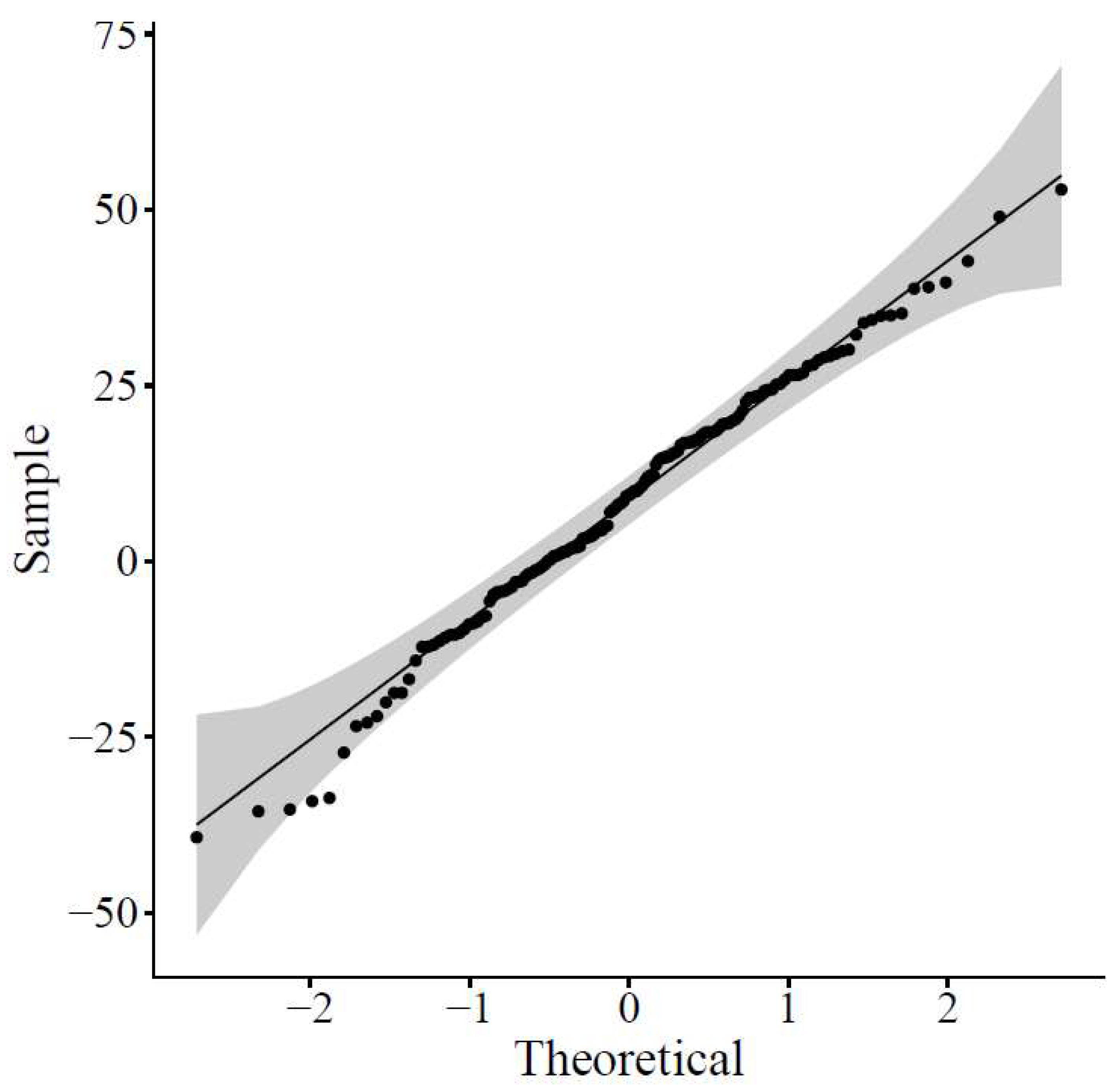
4.1. Aggregational Normality

As is well known, the S&P Composite Index benefits from aggregational normality. Accordingly, the null hypothesis of normally distributed rates of return has been rejected for monthly linear rates of return, both nominal and real, whereas it has not been rejected for annual linear rates of return, both nominal and real. The null hypothesis has also been rejected for monthly and annual logarithmic rates of return, both nominal and real. Our outcomes are in accordance with Nguyen et al. (2022), where the null hypothesis is rejected for the monthly returns on the stock market indices of the US, the UK, and Japan.
Jarque-Bera and Shapiro-Wilk tests have been performed using RStudio software: when a p-value is greater than 0.05, the null hypothesis is not rejected. Whatever the monthly rate of return, the p-values of both tests are lower than 2.2 × 10⁻¹⁶. The p-values for all annual rates are reported in Table 3.
Quantile-quantile plots have been constructed using RStudio software. For instance, the empirical distribution of the annual real rates of linear return is compared with a normal distribution in Figure 1. The confidence level of the shaded area is 0.95.
Non-overlapping multi-year rates of logarithmic return have also been examined. The p-values of Jarque-Bera and Shapiro-Wilk tests and the attendant quantile-quantile plots are not reported. The null hypothesis of normally distributed rates of return has been rejected for 2- and 3-year rates of logarithmic return, both nominal and real, whereas it has not been rejected for 4-year rates of logarithmic return, both nominal and real.
Therefore, the linear and logarithmic rates of return benefit from aggregational normality on two different time scales.

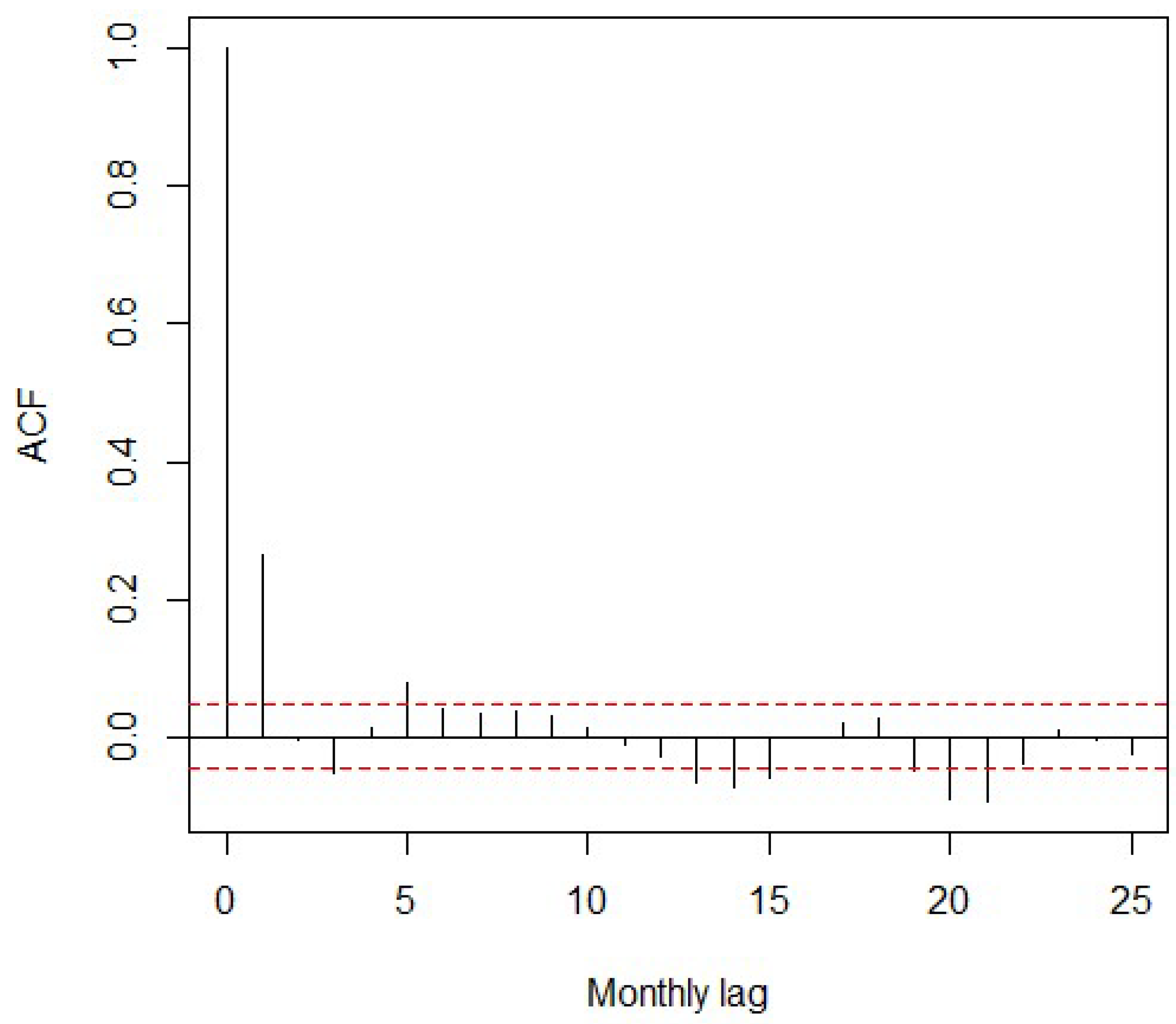
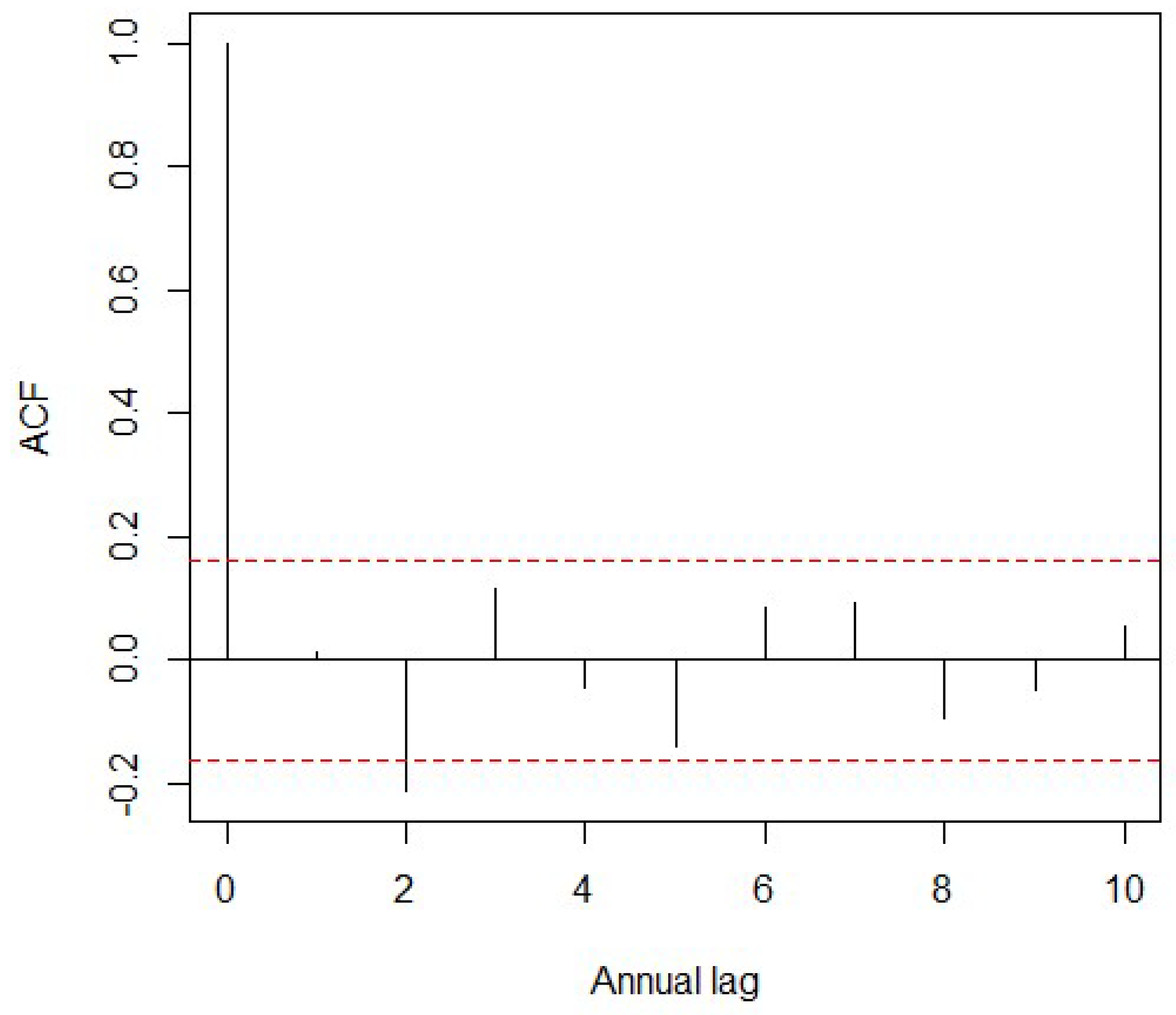
4.2. Serial Correlation

Sample autocorrelation functions have been estimated using RStudio software. The autocorrelation function for the monthly real rates of linear return is displayed in Figure 2. The unreported autocorrelation function for the monthly real rates of logarithmic return has a similar pattern.
Figure 2. Monthly real rates of linear return. Autocorrelation function.
Ijfs 11 00022 g002
The one-month autocorrelation is spurious; it is brought about by the S&P Composite data, which are monthly averages of daily closing values (Working 1960). Nonetheless, a few sample correlations lie outside the 0.95 confidence interval, the 5-month autocorrelation being positive and the 13-, 14-, 15-, 20-, and 21-month autocorrelations being negative.
The autocorrelation function for the annual real rates of linear return is displayed in Figure 3. The unreported autocorrelation function for the annual real rates of logarithmic return has a similar pattern. Only the 2-year autocorrelation lies outside the 0.95 confidence interval, being negative. Since Figure 2 and Figure 3 taken together are hard to interpret, a basic rescaled range analysis is performed in Section 4.3, whereas stationarity tests are performed in Section 5.2.

4.3. Rescaled Range Analysis

Use has been made of n = 149 12 = 1788 monthly real rates of logarithmic return from January 1872 to December 2020. The whole historical period has been divided into 1788 m subperiods, where m is the number of monthly observations that fall into each subperiod. Following Peters (1994), we have set m 10 , since a small m is not likely to be matched by a reliable estimate of the rescaled range R / S m . Iterating the procedure outlined in the Appendix A, the rescaled range R / S n has been estimated for n equal to m = 10 ,   20 ,   30 ,   ,   90 ,   100 months.
According to Hurst (1951), a British hydrologist, the exponent H obeys the equation
R / S m = c m H
so that it can be estimated by running the simple regression
l o g 10 R / S m = l o g 10 c + H l o g 10 m + error m
If both randomness and normality are assumed, the standard deviation of the resulting estimate H ^ is approximately 1 n = 1 1788 = 0.02365. Recall that the null hypothesis of normality has been previously rejected for all monthly rates of return.
The original theory allows one to distinguish between randomness H = 0.5 , a persistent trend 0.5 < H 1 , and an antipersistent trend 0 H < 0.5 . Randomness is represented by a sequence of independent and identically distributed random variables, in a persistent trend the next deviation from the mean is likely to have the present sign, and in an antipersistent trend the next deviation from the mean is likely to reverse the present sign. Persistent time series also display dependence between the remote past and the distant future owing to long-term memory; antipersistent time series reverse direction more often than random time series. For instance, Peters (1994) finds that the Dow Jones Industrial Average is a persistent time series by using the daily closing prices from 1888 to 1991. In contrast, he finds that the realized volatility of the S&P Composite Index is an antipersistent time series by using the daily prices from 1928 to 1989.
Unfortunately, a biased estimate H ^ may be obtained, since H ^ > 0.5 may be due to short-term memory rather than long-term memory. However, a heuristic remedy, reported by Peters (1994) and references therein, can reduce the risk of a biased estimate H ^ . Accordingly, the monthly real rates of logarithmic return have been replaced with the residuals of their autoregression of order 1; next, ten rescaled ranges have been estimated by iterating the procedure outlined in the Appendix A. Finally, the following Hurst exponent has been obtained from the simple regression (2):
H ^ = 0.64803
along with the coefficient of determination R 2 = 0.9972 . This outcome is hard to interpret owing to the heuristic procedure.
Suppose that the monthly real rates of logarithmic return form a sequence of identically distributed random variables. Adapting from Corazza and Malliaris (2002), we can now realize that for 0.5 < H 1 , such random variables may be either independent and Pareto-Lévy stable so that their variance is undefined, or not independent though fat-tailed. As stated by Campbell et al. (1997), if population variance is undefined and sample size is sequentially increased, sample variance does not approach a limiting value; Pareto-Lévy stability is preserved under addition. Therefore, the assumption of independent and Pareto-Lévy stable random variables is not tenable in light of the statistical tests of Section 4.1, whereby the 4-year real rates of logarithmic return are normally distributed.
Nonetheless, further analysis is required to ascertain whether the above-mentioned random variables are not independent though fat-tailed.
Borrowing from Hurst (1956), we have reconsidered the monthly real rates of logarithmic return and readily computed the running sum of the monthly departures from the mean, which is equal to 0.56%. Figure 4 displays such cumulative departures from the mean, which slowly fluctuate around the horizontal axis. In our opinion, Figure 4 complements Siegel (2014, p. 6), who observes: “Note that stocks fluctuate both below and above the trendline but eventually return to the trend. Economists call this behavior mean reversion, a property that indicates that periods of above-average returns tend to be followed by periods of below-average returns and vice versa.” Recall that such a trendline cannot be rigorously estimated by using elementary statistical methods.

5. Statistical Findings

5.1. Mean Blur

Let time be measured in years and S P t be the market value of a total real return stock index at the end of year t. Suppose that the total real return stock index follows a discrete-time random walk with constant parameters
l n S P t = l n S P t 1 + r t
where the error r t is an annual real rate of logarithmic return. Assume away the occurrence of structural breaks and suppose at first that the annual real rates of logarithmic return form a sequence of independent and normally distributed random variables. Let μ l o g and σ l o g be their constant and known population mean and standard deviation. Let n be the sample size and 0.95 be the confidence level. As is well known, the sample mean r ¯ l o g is normally distributed so that its confidence interval is
μ l o g 1.96 σ l o g n r ¯ l o g μ l o g + 1.96 σ l o g n
Therefore, the larger the sample size n, the narrower is the confidence interval. Unfortunately, increasing the sampling frequency is pointless. As hinted by Black (1993) and explained by Luenberger (2014), using a smaller unit of time does not help, since only the number of available years of data matters. For instance, if the monthly real rates of logarithmic return are considered, the sample size is larger and equal to 12 n . In contrast, the constant and known population mean and standard deviation are smaller and respectively equal to μ l o g 12 and σ l o g 12 . The confidence interval of the sample mean r ¯ ^ l o g 12 is
1 12 μ l o g 1.96 σ l o g n r ¯ l o g 12 1 12 μ l o g 1.96 σ l o g n
It is readily realised that the width of the confidence interval (6) is one-twelfth of the width of the confidence interval (5).
Suppose now that the annual real rates of logarithmic return form a sequence of independent and identically distributed random variables. Let now μ l o g and σ l o g be their constant and unknown population mean and standard deviation. Let s l o g be the sample standard deviation. As is well known, we have approximately
r ¯ l o g 1.96 s l o g n μ l o g r ¯ l o g + 1.96 s l o g n
provided that the sample size n is large enough.
According to Table 2, we have n = 149 as well as r ¯ l o g = 6.73 % and s l o g = 17.63 % . Substituting such values into the inequalities (7) gives
3.87 % μ l o g 9.59 %
which seems to be a case of mean blur, a definition given by Luenberger (2014). On considering only individual stocks, he concludes that reliable estimates of population means cannot be derived from historical rates of return, since too many years of data would be needed. However, he does not stress that mean blur is tacitly implied by the hypothesis of random walk (4) owing to high risk/reward ratios.
Both individual stocks and asset classes are considered by Haugen (1997, p. 171), who claims that, “For classes of securities, sample means of past rates of return are a good starting point for estimating future expected rates of return. Analysts usually start there, and then they make subjective adjustments to the estimates based on contemporary economic conditions which are now different from the past.” He adds that, “While sample mean returns serve as a good starting point in estimating the expected returns of classes of securities, they are poor indicators of differentials in expected return between securities within a class, such as common stocks. The past returns to individual stocks have been affected by myriad idiosyncratic events which are unlikely to repeat themselves in the future.”

5.2. Stationarity Tests

The hypothesis of random walk has been tested on 1788 monthly rates of logarithmic return. Unit root tests have been carried out by using RStudio software. According to both augmented Dickey-Fuller and Phillips-Perron tests, the null hypothesis of a unit root is rejected with a confidence level of 0.99 for both nominal and real rates of logarithmic return. Therefore, the total return version of the S&P Composite Index is trend-stationary rather than difference-stationary, both in nominal and real terms1. Our outcomes are consistent with the broader evidence provided by Nguyen et al. (2022) for the monthly returns on the stock market indices of the US, the UK, and Japan.
Additional stationarity tests have been performed to gain additional insight into mean blur. Use has been made of annual real rates of linear return, which meet the assumption of normality. Let μ l i n and σ l i n be their unknown population mean and standard deviation. At first, the historical period 1872–2020 has been divided into the two subperiods 1872–1935 and 1936–2020, respectively consisting of 64 and 85 years. The attendant sample moments are reported in Table 4.
Our first null hypothesis is that the sample means for both subperiods come from populations that have the same mean. The first null hypothesis is not rejected with a confidence level of 95 percent, since the two-sample t statistic takes the value
t = 0.032 < 1.655
Our second null hypothesis is that the sample variances for both subperiods come from populations that have the same variance. The second null hypothesis is not rejected with a confidence level of 95 percent, since the F statistic takes the value
F = 1.139 < 1.468
Next, a single factor analysis of variance (ANOVA) has been performed. Therefore, the historical period 1872–2020 has been divided into the three subperiods 1872–1911, 1912–1970, and 1971–2020, respectively consisting of 40, 59 and 50 years. The attendant sample moments are reported in Table 5.
Our null hypothesis is now that the sample means for all three subperiods (or groups) come from populations that have the same mean. The null hypothesis is provisionally not rejected with a confidence level of 95 percent, since the F statistic takes the value
F = variance   between   groups variance   within   groups = 0.002 < 3.058
Unfortunately, the null hypothesis of homoskedasticity is rejected with a confidence level of 95 percent, since Bartlett’s statistic takes the value
χ 2 = 8.1039 > 0.103
The attendant p-value is equal to 0.01736, implying that heteroskedasticity is not strong. Indeed, the range of the sample means in Table 5 is narrow, whereas the range of the sample standard deviations in Table 5 is broad. However, small samples are involved so that the long-run stationarity of variance is an issue that would require further examination. In doing so, the role played by structural breaks should not be disregarded.
Nonetheless, Equation (8) seems to clash with Equations (9) and (10) as well as with the previous unit root tests. In our opinion, this is further evidence that the annual real rates of return are not independent owing to mean reversion so that the unknown standard deviation of the sample mean is lower than
σ l i n n
as tacitly assumed.
Remarkably, other evidence was provided by Poterba and Summers (1988), who also analyzed the performance of the S&P Composite Index over the years 1871–1985 by making a comparison between different multi-year real rates of logarithmic return and the one-year real rates of logarithmic return. According to the variance-ratios of their Table 3, the annualized variances of the former are lower than the variance of the latter. Unfortunately, statistical significance is hard to attain. Recall that the above-mentioned variances are proportional to the sampling interval under the assumption of random walk, whereas they are less than proportional to the sampling interval under the assumption of mean reversion.

6. Conclusions

This study has used a very long time series of the S&P Composite Index, checking once more that the annual rates of linear return, both nominal and real, benefit from aggregational normality. It has stressed that the hypothesis of random walk with constant parameters implies that means are very blurred owing to high risk/reward ratios so that they cannot be estimated by using statistical methods. It has performed unit root tests on the S&P Composite Index as well as elementary statistical tests that take advantage of normality. It has ascertained that the means of the annual real rates of linear return are not very blurred. This is further evidence that the annual real rates of return are not independent, owing to mean reversion.
Therefore, when it comes to stock indices (and well-diversified stock portfolios), mean reversion may lessen mean blur. Although our statistical evidence is preliminary, it can be corroborated by performing the same elementary statistical tests on very long time series of other stock indices. Keep in mind that our study has the limitation of not dwelling on past structural breaks.
Owing to their clarity and simplicity, the above-mentioned elementary statistical tests may be useful both in teaching and business practice. Indeed, the late Fischer Black was keen on telling the truth and explaining quantitative models to traders in simple terms (Dunbar and Dunbar 2001).

Author Contributions

Conceptualization, L.B. and L.G.; Methodology, L.B. and L.G.; Writing—original draft, L.B. and L.G. All authors have read and agreed to the published version of the manuscript.

Funding

This research received no external funding.

Institutional Review Board Statement

Not applicable.

Informed Consent Statement

Not applicable.

Data Availability Statement

Raw data downloaded from www.econ.yale.edu/~shiller/data.htm.

Acknowledgments

We are grateful to Elena Conti for her editorial support and to Laura Ballestra for her bibliographical assistance. We also thank two anonymous reviewers for their useful comments and suggestions. As usual, we are solely responsible for any remaining errors.

Conflicts of Interest

The authors declare no conflict of interest.

Appendix A

Let m = 12 so that 1788 12 = 149 subperiods are available. Compute each year a monthly mean, a monthly standard deviation, m = 12 monthly deviations from the mean, a partial (or running) sum of such deviations, a range, namely the difference between the positive maximum and the negative minimum of the running sum, and the ratio between range and standard deviation.
Next, obtain the rescaled range R / S 12 by averaging 149 ratios between range and standard deviation.

Note

1
As remarked by an anonymous reviewer, the above-mentioned unit root tests may be misleading whenever data are affected by structural breaks. According to the Zivot-Andrews test, the null hypothesis of a unit root is rejected once more with a confidence level of 0.99 for real rates of logarithmic return. A structural break occurring in July 2000 has been detected, which is in line with Table 5 in Nguyen et al. (2022). The same authors summarize the relevant econometric literature.

References

  1. Black, Fischer. 1993. Estimating expected return. Financial Analysts Journal 49: 36–38. [Google Scholar] [CrossRef]
  2. Buffett, Warren, and Carol Loomis. 2001. Warren Buffett on the Stock Market. Fortune 144: 40–46. [Google Scholar]
  3. Campbell, John Y., and Robert J. Shiller. 1998. Valuation ratios and the long-run stock market outlook. Journal of Portfolio Management 24: 11–26. [Google Scholar] [CrossRef]
  4. Campbell, John Y., Andrew W. Lo, and A. Craig MacKinlay. 1997. The Econometrics of Financial Markets. Princeton: Princeton University Press. [Google Scholar]
  5. Corazza, Marco, and Anastasios G. Malliaris. 2002. Multifractality in foreign currency markets. Multinational Finance Journal 6: 387–401. [Google Scholar] [CrossRef]
  6. Cornell, Bradford. 2010. Economic growth and equity investing. Financial Analysts Journal 66: 54–64. [Google Scholar] [CrossRef]
  7. Dunbar, Nicholas, and Nick Dunbar. 2001. Inventing Money. The Story of Long-Term Capital Management and the Legends behind it. Chichester: Wiley. [Google Scholar]
  8. Fama, Eugene F., and Kenneth R. French. 1988a. Permanent and temporary components of stock prices. Journal of Political Economy 96: 246–73. [Google Scholar] [CrossRef]
  9. Fama, Eugene F., and Kenneth R. French. 1988b. Dividend yields and expected stock returns. Journal of Financial Economics 22: 3–25. [Google Scholar] [CrossRef]
  10. Golez, Benjamin, and Peter Koudijs. 2018. Four centuries of return predictability. Journal of Financial Economics 127: 248–63. [Google Scholar] [CrossRef] [Green Version]
  11. Haugen, Robert A. 1997. Modern Investment Theory, 4th ed. Upper Saddle River: Prentice-Hall. [Google Scholar]
  12. Hurst, Harold E. 1956. The problem of long-term storage in reservoirs. Hydrological Sciences Journal 1: 13–27. [Google Scholar] [CrossRef] [Green Version]
  13. Hurst, Harold Edwin. 1951. The long-term storage capacity of reservoirs. Transactions of the American Society of Civil Engineers 116: 770–99. [Google Scholar] [CrossRef]
  14. Lo, Andrew W., and A. Craig MacKinlay. 1988. Stock market prices do not follow random walks: Evidence from a simple specification test. Review of Financial Studies 1: 41–66. [Google Scholar] [CrossRef]
  15. Loomis, Carol, and Warren Buffett. 1999. Mr. Buffett on the Stock Market. Fortune 140: 110–15. [Google Scholar]
  16. Luenberger, David G. 2014. Investment Science, 2nd ed. New York: Oxford University Press. [Google Scholar]
  17. Maginn, John L., Donald L. Tuttle, Dennis W. McLeavey, and Jerald E. Pinto. 2007. The portfolio management process and the investment policy statement. In Managing Investment Portfolios. A Dynamic Process, 3rd ed. Edited by John L. Maginn, Donald L. Tuttle, Dennis W. McLeavey and Jerald E. Pinto. Hoboken: Wiley, pp. 1–19. [Google Scholar]
  18. Nguyen, James, Wei-Xuan Li, and Clara Chia-Sheng Chen. 2022. Mean Reversions in Major Developed Stock Markets: Recent Evidence from Unit Root, Spectral and Abnormal Return Studies. Journal of Risk and Financial Management 15: 162. [Google Scholar] [CrossRef]
  19. Peters, Edgar E. 1994. Fractal Market Analysis. New York: Wiley. [Google Scholar]
  20. Poterba, James M., and Lawrence H. Summers. 1988. Mean reversion in stock prices: Evidence and implications. Journal of Financial Economics 22: 27–59. [Google Scholar] [CrossRef]
  21. Royal Swedish Academy of Sciences. 2013. Trendspotting in Asset Markets. Available online: https://www.nobelprize.org/uploads/2018/06/popular-economicsciences2013.pdf (accessed on 4 March 2022).
  22. Sharpe, William F., Peng Chen, Jerald. E. Pinto, and Dennis. W. McLeavey. 2007. Asset allocation. In Managing Investment Portfolios. A Dynamic Process, 3rd ed. Edited by John L. Maginn, Donald L. Tuttle, Dennis W. McLeavey and Jerald E. Pinto. Hoboken: Wiley, pp. 230–327. [Google Scholar]
  23. Shiller, Robert J. 2015. Irrational Exuberance, 3rd ed. Princeton: Princeton University Press. [Google Scholar]
  24. Siegel, Jeremy J. 2014. Stocks for the Long Run, 5th ed. New York: McGraw-Hill. [Google Scholar]
  25. Spierdijk, Laura, and Jacob A. Bikker. 2017. Mean reversion in stock prices: Implications for long-term investors. In Pension Fund Economics and Finance. Efficiency, Investments and Risk-Taking. Edited by Jacob Bikker. London: Routledge. [Google Scholar]
  26. Summers, Lawrence H. 1986. Does the stock market rationally reflect fundamental values? Journal of Finance 41: 591–601. [Google Scholar] [CrossRef]
  27. von Hippel, Paul T. 2005. Mean, median, and skew: Correcting a textbook rule. Journal of Statistics Education 13. [Google Scholar] [CrossRef] [Green Version]
  28. Working, Holbrook. 1960. Note on the correlation of first differences of averages in a random chain. Econometrica 28: 916–18. [Google Scholar] [CrossRef]
Figure 1. Annual real rates of linear return. Quantile-quantile plot.
Ijfs 11 00022 g001
Figure 3. Annual real rates of linear return. Autocorrelation function.
Ijfs 11 00022 g003
Figure 4. Monthly real rates of logarithmic return. Cumulative departures from the mean.
Ijfs 11 00022 g004
Table 1. Monthly real rates of return, 1872–2020.
Linear Rate Logarithmic Rate
Worst rate−26.19%−30.36%
Median0.94%0.94%
Best rate52.43%42.15%
Negative rates39.21%39.21%
Mean0.65%0.56%
Standard deviation4.10%4.08%
Skewness0.58−0.36
Kurtosis excess18.2411.38
Raw data downloaded from www.econ.yale.edu/~shiller/data.htm (accessed date: 4 March 2022).
Table 2. Annual real rates of return, 1872–2020.
Linear RateLogarithmic Rate
Worst rate−39.29%−49.90%
Median10.01%9.54%
Best rate53.25%42.69%
Negative rates30.87%30.87%
Mean8.55%6.73%
Standard deviation17.98%17.63%
Skewness−0.29−0.83
Kurtosis excess0.030.92
Raw data downloaded from www.econ.yale.edu/~shiller/data.htm (accessed date: 4 March 2022).
Table 3. Annual rates of p-values.
RateJarque-BeraShapiro-Wilk
Linear0.34940.5082
Logarithmic3.741 × 10−60.00021
Real Linear0.35950.3214
Real Logarithmic2.501 × 10−50.0001341
Table 4. Annual real rates of linear return, 1872–2020, two subperiods.
1872–20201872–19351936–2020
Worst rate−39.29%−36.66%−39.29%
Median10.01%4.90%11.98%
Best rate53.25%53.25%49.16%
Negative rates30.87%32.81%29.41%
Mean8.55%8.61%8.51%
Standard deviation17.98%18.70%17.53%
Skewness−0.29−0.04−0.52
Kurtosis excess0.030.010.10
Raw data downloaded from www.econ.yale.edu/~shiller/data.htm (accessed date: 4 March 2022).
Table 5. Annual real rates of linear return, 1872–2020, three subperiods.
1872–20201872–19111912–19701971–2020
Worst rate−39.29%−27.94%−36.66%−39.29%
Median10.01%7.96%7.45%12.29%
Best rate53.25%40.53%53.25%34.99%
Negative rates30.87%27.50%35.59%28.00%
Mean8.55%8.67%%8.82%8.14%
Standard deviation17.98%14.27%21.39%16.51%
Skewness−0.29−0.04−0.09−0.94
Kurtosis excess0.03−0.05−0.550.69
Raw data downloaded from www.econ.yale.edu/~shiller/data.htm (accessed date: 4 March 2022).
Disclaimer/Publisher’s Note: The statements, opinions and data contained in all publications are solely those of the individual author(s) and contributor(s) and not of MDPI and/or the editor(s). MDPI and/or the editor(s) disclaim responsibility for any injury to people or property resulting from any ideas, methods, instructions or products referred to in the content.

