The Relationship between Contraction of the Ejector Mixing Chamber and Supersonic Jet Mixing Layer Development

Abstract

Supersonic mixing layer development seriously impacts on the performance of an ejector, and the effect of mixing chamber contraction angle on supersonic jet mixing has been poorly studied. Numerical simulations are applied to investigate the effect of the mixing chamber contraction angle (φ) on the performance of a central ejector and supersonic mixing layer development pattern. The main findings of this study are as follows: the non-mixed length (l) is reduced by 22.12% when the mixing chamber contraction angle (φ) increases from 2° to 6°. Meanwhile, the secondary stream mass flow rate (m_s) is reduced by 35.02%, and the total pressure loss is decreased by 18.37% at the outlet. l is positively correlated with m_s and negatively correlated with the mixing layer thickness (σ). The mixing layer thickness (σ) grows highly linearly before the secondary flow is covered completely. The pressurization (P_0δ/P_0s) performance of the mixing layer will be progressively weaker than the total pressure loss because of the complex shock structure.

1. Introduction

The ejector is a fluid pump without complex moving parts. By the convection and viscous shear between fluids, the kinetic energy of the induced working fluid is increased, and the mass mixing between fluids is achieved. The first ejector in the world was invented in the middle of the 19th century to replace mechanical pumps for boiler water delivery. Structural simplicity, large entrainment ratio and low cost are the main advantages of the central ejector. Therefore, it has numerous applications in chemical [1,2], aerospace [3,4] and new energy [5,6] fields.

Numerous studies have been carried out by domestic and international scholars on central ejectors. The two basic configurations are the constant area mixing (CAM) ejector and the constant pressure mixing (CPM) ejector [7]. Most studies related to the central ejector have been developed based on the configuration of CAM and CPM. The entrainment ratio (ER) and compression ratio (CR) are essential parameters to evaluate the performance of the ejector. Research has shown that various factors influence the performance of the central ejector. The primary flow nozzle exit position (NXP) is one of the significant impact factors. With too large an NXP, the ER will be substantially declined [8]. Chunnanond and Aphornratana [9] have explained the effect of NXP on ER by analyzing the expansion angle and effective mixing area. In addition, excessive NXP leads to a more serious boundary layer separation, where the mixed fluid is unlikely to overcome the back pressure discharge, and the ejector fails to start [10]. Several works have identified the optimum location for NXP and discussed the factors that affect it [11,12,13]. Furthermore, the primary to secondary flow area ratio [12] and mixing chamber length [14] also have a great influence on the performance of the central ejector. In the past series of studies, angles such as 0.5° [15], 1° [16] and 1.45–4.2° [17] have been used as the optimal mixing chamber contraction angles. In order to improve the ER or CR, some works on the optimized design of the ejector were carried out [18,19,20,21,22].

Contrary to conventional supersonic jet mixing [20], the development of the ejector mixing layer is greatly limited by the space constraints. Some works were carried out in the area of ejector supersonic mixing layer. Bartosiewicz et al. [23] investigated the variation of the non-mixed length for different primary and secondary flow pressureand found that the SST k-ω turbulence model has a better calculation performance for flow mixing. Rao et al. [24] quantified the non-mixed length from flow visualization images and found l to be 4.5–5.2 times the height of the mixing flow channel. Subsequent studies [20] have found that the development of the mixing layer has a significant impact on the performance of the ejector. Ka A et al. [25] investigated the development of a supersonic mixing layer through numerical simulation and experimental methods. They found that the compression effect of the mixing layer was reduced, and the growth rate of the mixing layer was accelerated when the pressure of the secondary flow increased. Tang Y et al. [26] conducted a related study by numerical simulation, and the results showed that the supersonic mixing layer thickness grows in a fluctuating state at the beginning and then grows exponentially. When the mixing layer grows more rapidly, the entrainment ratio is higher, indicating that the secondary flow is more easily mixed into the primary flow. Primary stream condensation in the steam ejector results in faster mixing layer growth [27]. Increased mixing efficiency between the primary and secondary flow is the principal reason for the higher entrainment ratio.

Currently, related studies have focused on the relationship between dimensional structural parameters, state parameters of the working substance and local flow phenomenon with the performance of the central ejector. Convection and blending between the primary and secondary flow is a complicated process. The development and thickness growth of the supersonic mixing layer reflect the mixing ability between the primary and secondary flow. The non-mixed length, the thickness of the mixing layer and the pressurization pattern within the mixing layer are closely related to the performance of the ejector. Research on the supersonic mixing layer can help optimize the design of the ejector structure size, thus achieving material savings and weight reduction. In aerospace, it is critical to reduce the weight of the ejector. Adequate understanding of the supersonic mixing layer development will enable us to recognize the mixing process of the primary and secondary flow in essence. Thus, it is possible to obtain the origin of the variation in the performance of the ejector and extract more details on the optimization of the ejector.

Accordingly, the study was carried out in this article using a numerical simulation method. From the previous research experience and the practical significance of engineering applications [18,19,20], different mixing chamber contraction angles (φ) of 0°, 2°, 4° and 6° were set. Then, we investigated the development process concerning the boundary and thickness of the supersonic mixing layer and the pressurization pattern within the mixing layer.

2. Research Methodology and Process

The detailed discussion in this chapter is carried out in five aspects: the physical model, assessment parameters, solution method, numerical validation and grid sensitivity analysis. The specific process of obtaining experimental results is described and ensures the accuracy of the numerical simulation outcomes.

2.1. Physical Model

The central ejector configuration used in this numerical simulation can be seen in Figure 1. The computational domain includes the primary flow nozzle, secondary flow channel and mixed flow channel (both the mixing chamber and secondary throat). In this numerical simulation, different operating conditions were formulated by setting varying contraction angles (φ) of the mixing chamber. The boundary conditions and structural parameters are detailed in

Table 1. Boundary condition parameters.

Case	φ (°)	P0p (MPa)	T0p (K)	T0s (K)	P0s (kPa)	Pout (kPa)	L
1	0	4.0	300	300	20	0	10D
2	2
3	4
4	6

. A few conditions are not included in the table: mixing chamber contraction ratio A_t/A₀ = 0.6, and the primary and secondary flow work gas is air and nitrogen, respectively. D in Table 1 is the diameter of the mixing flow channel when φ = 0°. Figure 2 shows all configurations.

2.2. Assessment Parameters

The secondary flow mass fraction is used to define the mixing boundary. Therefore, the primary and secondary flow boundaries of the mixing layer correspond to the secondary flow mass fraction equal to 90% and 10% [27], respectively. The influence of the mixing chamber contraction angle on the development of the mixing layer will be investigated by the following parameters: the non-mixed length (l), supersonic mixing layer boundary position and the mixing layer thickness (δ). Each of these evaluation parameters is clearly labeled in Figure 3. The average total pressure (P_0δ) at a position within the mixed layer is extracted, and its ratio to the secondary flow total pressure is P_0δ/P_0s. This value represents the pressure increment effect of the primary flow on the secondary flow.

2.3. Solution Method and Turbulence Model

The density is changing during the mixing of the primary and secondary streams in the ejector. So, the Favre-averaged Navier–Stokes equations are more suitable and will be used in this work. The total energy equation is coupled to the perfect gas law, and the thermodynamic and transport properties of the air remain unchanged; validation runs show that they have a minor effect. The governing equations can be expressed as follows [28]:

$$\frac{\partial \rho }{\partial \mathrm{t}}+\frac{\partial }{\partial {\mathrm{x}}_{\mathrm{i}}}\left(\rho {\mathrm{U}}_{\mathrm{i}}\right)=0$$

(1)

$$\frac{\partial }{\partial \mathrm{t}}\left(\rho {\mathrm{U}}_{\mathrm{i}}\right)+\frac{\partial }{\partial {\mathrm{x}}_{\mathrm{i}}}\left(\rho {\mathrm{U}}_{\mathrm{i}}{\mathrm{U}}_{\mathrm{j}}\right)=-\frac{\partial \mathrm{P}}{\partial {\mathrm{x}}_{\mathrm{i}}}+\frac{\partial {\tau }_{\mathrm{ij}}}{\partial {\mathrm{x}}_{\mathrm{j}}}$$

(2)

$$\frac{\partial }{\partial \mathrm{t}}\left(\rho \mathrm{E}\right)+\frac{\partial }{\partial {\mathrm{x}}_{\mathrm{i}}}\left({\mathrm{U}}_{\mathrm{i}}\right(\rho \mathrm{E}+\mathrm{P}\left)\right)=\overrightarrow{\nabla }·\left({\alpha }_{\mathrm{eff}}\frac{\partial \mathrm{T}}{\partial {\mathrm{x}}_{\mathrm{i}}}+{\mathrm{U}}_{\mathrm{j}}({\tau }_{\mathrm{ij}})\right)$$

(3)

$$\rho =\frac{\mathrm{P}}{\mathrm{RT}}$$

(4)

$${\tau }_{\mathrm{ij}}={\mu }_{eff}\left(\frac{\partial u_i}{\partial x_j}+\frac{\partial u_i}{\partial x_i}\right)-\frac{2}{3}{\mu }_{eff}\frac{\partial u_k}{\partial x_k}{\sigma }_{ij}$$

(5)

Among many turbulence models, the RNG and k-omega SST turbulence models were best suited to predict the shock phase, strength and the mean line of pressure recovery [23,29]. However, the k-omega SST turbulence further showed better performances in terms of stream mixing. So, the SST k-ω turbulence model is used to tackle the relevant turbulence parameters. The ANSYS Fluent18.0 simulation platform is used and combined with the implicit density-based solver for steady-state numerical calculations. The wall boundary is treated as adiabatic and nonslip [6], and the standard wall function is applied near the walls [30]. A second-order upwind scheme is selected to achieve a high order of accuracy. For the turbulence variable boundary conditions, the hydraulic diameter is set to the diameter of the outlet or inlet, and the turbulence intensity is the default value.

The calculation can be considered convergent when both of the following conditions are met: (a) every type of calculated residual error must be less than 10⁻⁶; (b) the relative difference of mass flow rate between the inlet and outlet boundaries must be less than 0.001.

2.4. Numerical Validation

In general, since the turbulence model chosen for the numerical simulation can accurately calculate the near-wall pressure and the entrainment ratio, then the chosen model can be considered reliable [31]. Al-Doori’s [32] ejector and experimental results [27] are selected as criteria for the numerical validation in this study. As can be seen from

Table 2. Comparison of numerical simulation and experimental results of the induced coefficients.

Condition	P0p (kPa)/T0p (K)	P0s (kPa)/T0s (K)	Pout (kPa)/Tout (K)	Entrainment Ratio	Error (%)
Experimental	270/403	1.2/283	6/403	0.33	--
Simulation				0.347	5.15

, the mass flow rates of the selected calculation cases agree fairly well with their experimental values, and the prediction error is less than 10%. A comparison of the experimentally measured near-wall pressure distribution and the calculated value is shown in Figure 4. Again, we can observe that the numerical calculation results deviate slightly from the experimental results.

The results above fully demonstrate that the model used in this numerical simulation can accurately simulate the overall performance and local flow characteristics of the ejector.

2.5. Meshing Generation and Grid Sensitivity Analysis

For the central ejector, numerical calculations using a 2D axisymmetric model instead of a 3D model are theoretically able to obtain accurate results. The irrelevance validation of the 3D and 2D axisymmetric models is carried out using the same number and arrangement of nodes in Case1 as an example. Here, we can test whether there is any difference between the 3D model and the 2D axisymmetric model. ANSYS ICEM is applied to mesh the computational fluid domain, and the mesh is encrypted at near-wall areas, as depicted in Figure 5.

Table 3. Three-dimensional/two-dimensional model calculation results and errors.

Model	mp (kg/s)	Error-p (‰)	ms (kg/s)	Error-s (‰)
3d	7.49691	--	1.06458	--
2d	7.49499	0.26	1.06657	1.87

shows the calculation results and errors of different models.

In Figure 6, the central axis velocity development and wall static pressure variation curves are compared for the 3D and 2D axisymmetric calculation models. It is obvious that the calculation results of the 2D and 3D models are highly consistent under the design conditions. In summary, for the axisymmetric configuration of the central ejector, the 2D model can obtain the same accurate results as the 3D model. In order to save computational resources and numerical simulation time, the 2D axisymmetric model is used for numerical calculations of all working conditions in this study.

The ejector fluid domain is initially divided into 49,497 structured meshes. A grid sensitivity analysis is carried out to avoid grid density variations from affecting the calculation results. In Case1, as a typical example, four grid models with the same topological complement structure and smooth grid transition are set. Grid numbers, calculation results and error comparisons are shown in

Table 4. Grid independence analysis results.

Grid Label	Grid Number	mp (kg/s)	Error-p (‰)	ms (kg/s)	Error-s (‰)
Grid1	49,497	8.4692	--	1.004	--
Grid2	96,883	8.4672	0.24	1.003	1.0
Grid3	185,577	8.4673	0.01	1.004	1.0
Grid4	330,301	8.4681	0.09	1.004	0.0

and Figure 6.

As can be seen from Table 4, when the grid number reaches 185,577 (Grid3), the mass flow rate changes minimally. When continuing to encrypt the grid number to 330,301 (Grid4), the primary and secondary stream mass flow rates trend toward stabilization. Figure 7 shows the consistent trend in the mixing layer thickness of Grid1~4. However, Grid1 and Grid2 are slightly lacking in the ability to capture the details of the mixing layer.

Error accumulation is inevitable due to the finite grid size of successive time steps. The effect of grid size on error accumulation is investigated in this study using the method developed by Smirnov et al. [33,34]. The relative error of integration in the i direction (S_i) is proportional to the mean ratio of cell size (Δl) to the domain size (l_i); for a uniform grid, it could be

$$S_i\approx {\left(\Delta l/l_i\right)}^{k+1}={\left(1/N_i\right)}^{k+1}$$

(6)

where k is the order of accuracy of the numerical scheme; in the present simulations, the spatial discretization with a second-order scheme is applied; N_i is the number of cells in the direction of integration. The integration errors S_err are the sum of S_i in all directions:

$$S_{err}\approx {\displaystyle \sum _{i=1}^3{S}_i}$$

(7)

The maximum allowable number of time steps n_max can be decided by

$$n_{\max }={\left(S_{\max }/S_{err}\right)}^2$$

(8)

in which S_max is the allowable value of total error; it is presumed to be 1% in the present study. Then, a ration coefficient R_s is introduced to quantify the reliability of the results:

$$R_s=n_{\max }/n$$

(9)

Herein, n represents the actual number of integration steps. The details for error accumulation for the three grid resolutions are tabulated in

Table 5. Grid independence analysis results.

Grid Label	S1	S2	Serr	Smax	n	nmax	Rs
Grid1	8.87 × 10−09	7.51 × 10−07	7.60 × 10−07	0.01	500,000	1.73 × 108	346.09
Grid2	3.19 × 10−09	2.90 × 10−07	2.94 × 10−07	0.01	500,000	1.16 × 109	2319.48
Grid3	1.37 × 10−09	1.00 × 10−07	1.02 × 10−07	0.01	500,000	9.61 × 109	19,226.46
Grid4	4.78 × 10−10	5.20 × 10−08	5.24 × 10−08	0.01	500,000	3.64 × 1010	72,758.58

. Results show that the R_s coefficients for both cases are much greater than unity, demonstrating that their accumulation errors will not exceed the maximal allowable values.

In order to strike a proper balance between the computational load and prediction accuracy, the grid number is taken in a value of 185,577.

3. Results and Discussion

In this section, the effect of the mixing chamber contraction angle (φ) on the mixing layer development pattern is carefully explored based on the evaluation parameters presented in Section 2.2. Furthermore, the fundamental relationship between φ, the supersonic mixing layer evolution pattern and the performance of the ejector is further revealed.

3.1. Variation of Supersonic Mixing Layer Boundary

The static pressure at the center of the primary flow (P_p) is about 21.3 kPa at the nozzle exit section. In all operating conditions, the state parameters of the primary flow will not change with φ. When φ increases from 0° to 6°, the static pressure of the secondary flow (P_s) at the nozzle exit section gradually increases. Additionally, the static pressure ratio P_s/P_p increases from about 0.75 to 0.89. Therefore, the under-expanded primary flow dictates that the secondary flow boundary will gradually develop up to the wall of the mixing chamber.

As shown in Figure 8, the position of the secondary flow covered point x_t decreases from 909.1 mm to 552 mm when φ gradually expands. Compared with φ = 2°, the non-mixed length l is reduced by 22.12% for φ = 6°. The secondary flow boundary is more curved and closer to the axial direction at a mixing chamber contraction angle of 2°, 4° or 6°. Thus, the secondary flow boundary is slightly compressed. There are two main reasons for this phenomenon. First, the increased contraction angle reduces the distance from the primary flow nozzle outlet to the wall of the mixing chamber. Then, the secondary flow boundary is more likely to develop to the wall of the mixing chamber, as in Figure 8a. Second, a larger mixing chamber contraction angle will bring higher secondary flow static pressure at the nozzle exit section (Figure 8b). The mixing layer is subject to stronger compression at this time. Figure 9 shows the mass fraction distribution of the primary and secondary flows, and it can be more clearly visualized that the non-mixed length l decreases with the increase in φ.

Different to the secondary flow, the boundary of the primary flow is distinct in its development. Figure 10a shows the development of the primary flow boundary of the mixing layer for different mixing chamber contraction angles. At the beginning of the mixing of the primary and secondary streams, the higher static pressure of the primary stream makes it develop outward first. The development of the primary flow boundary along the radial direction is maximum when the contraction angle of the mixing chamber φ = 0°. With a gradually increasing φ, the initial development of the primary flow boundary along the radial direction is severely inhibited (Figure 10, region A). Additionally, when the mixing layer develops inside the secondary throat, the primary flow boundary tends to smooth out. At this time, the primary flow boundary shows fluctuations due to the penetration of the complicated wave structure. Figure 10b depicts the relationship between the secondary stream mass flow rate (m_s) and the non-mixed length l. It can be observed that m_s gradually increases when the non-mixed length l grows. Thus, m_s has a positive correlation with the non-mixed length l.

The primary flow boundary developments at φ = 0° are shown in Figure 11. Numerical Schlieren image and pressure distribution comparisons are appended to Figure 11 for better interpretation of the primary flow boundary fluctuations. In the graph, RS₁-RS₆ are oblique shock waves in the primary flow, and TS₁-TS₄ are oblique shock waves within the mixing layer. Obviously, the shock wave strength RS₁ > RS₂ > TS₁ > TS₂ > RS₃ > RS₄ > TS₃ > TS₄ > RS₅ > RS₆. The following analysis explains the fluctuating state exhibited by the development of the primary flow boundary.

Before the oblique shock wave RS₁, the primary flow passes through a series of expansion waves, decreasing its static pressure. A sudden increase in static pressure is observed after the shock wave RS₁. Therefore, during section AB, the static pressure within the mixing layer is relatively lower, enabling the primary flow boundary to develop toward the wall. Due to the energy and mass transfer between the primary and secondary flows, more high-energy primary flow enters the mixing layer. Additionally, the static pressure in the mixing layer keeps increasing. At spot B, the static pressure of the fluid is equal on both sides of the primary flow boundary. The static pressure is lower on the primary flow side, which turns it into a compressed state (section BC).

For the oblique shock waves RS₂ and TS₁, the intensity of RS₂ is stronger. Additionally, the primary velocity is greater than that in the mixing layer. A larger static pressure value increase is observed in the primary flow after the oblique shock wave RS₂. Again, the primary flow boundary develops toward the wall in section CD. For the oblique shock waves TS₂ and RS₃, the intensity of TS₂ is higher, and its static pressure increment to the mixing layer is much greater. In section DE, the primary flow boundary is again compressed.

For the reasons above, in sections EF and FG, the magnitude of the static pressure increment after the fluid passes through the oblique shock wave determines whether the primary flow boundary develops outward or becomes compressed.

3.2. Growth and Pressurization Performance of the Mixing Layer

The thickness and pressure variations of the mixed layer reflect the mass and energy transfer pattern between the primary and secondary flows. Therefore, it is worthwhile to analyze the thickness of the mixing layer and the pressurization performance.

Figure 12 represents the development of the mixing layer thickness (σ) along the range for different φ. In the early stages of mixing layer development, i.e., in the range of the non-mixed length l, the mixing layer thickness (σ) increases linearly. Additionally, it grows in a faster linear fashion as φ increases. The result is that a large mixing chamber contraction angle promotes the growth of the mixing layer. Noticeably, the convective Mach number also varies in a small range when φ is changed from 0° to 6°, i.e., M_c = 1.2~1.1. Ka A et al. [23] also found the quasilinear growth pattern of the mixing layer thickness at convective Mach number Mc = 1.4. The convective Mach number is a significant dimensionless parameter for characterizing the compressibility of a fluid and is defined as

$$Mc=\frac{\Delta U}{a_1+a_2}$$

(10)

where ΔU is the velocity difference of two streams across the mixing layer; a₁ and a₂ are the speed of sound for both sides of the mixing layer of the primary and secondary flows.

The mixing layer grows linearly, followed by the fluctuating states of slow growth. Fluctuations are more dramatic as the thickness of the mixing layer grows to a greater φ. From region A, we can see that the thickness of the mixing layer gradually increases as the non-mixed length l decreases. It shows that l is negatively correlated with the mixing layer thickness δ. The interaction of the complicated wave structure with the mixing layer is the main reason for its thickness fluctuation (a detailed explanation is elaborated in Section 3.1). Compared with φ = 0°, when φ = 2°, 4°, 6°, a new oblique shock wave will be generated to render the structure of the original wave system more complicated (Figure 13).

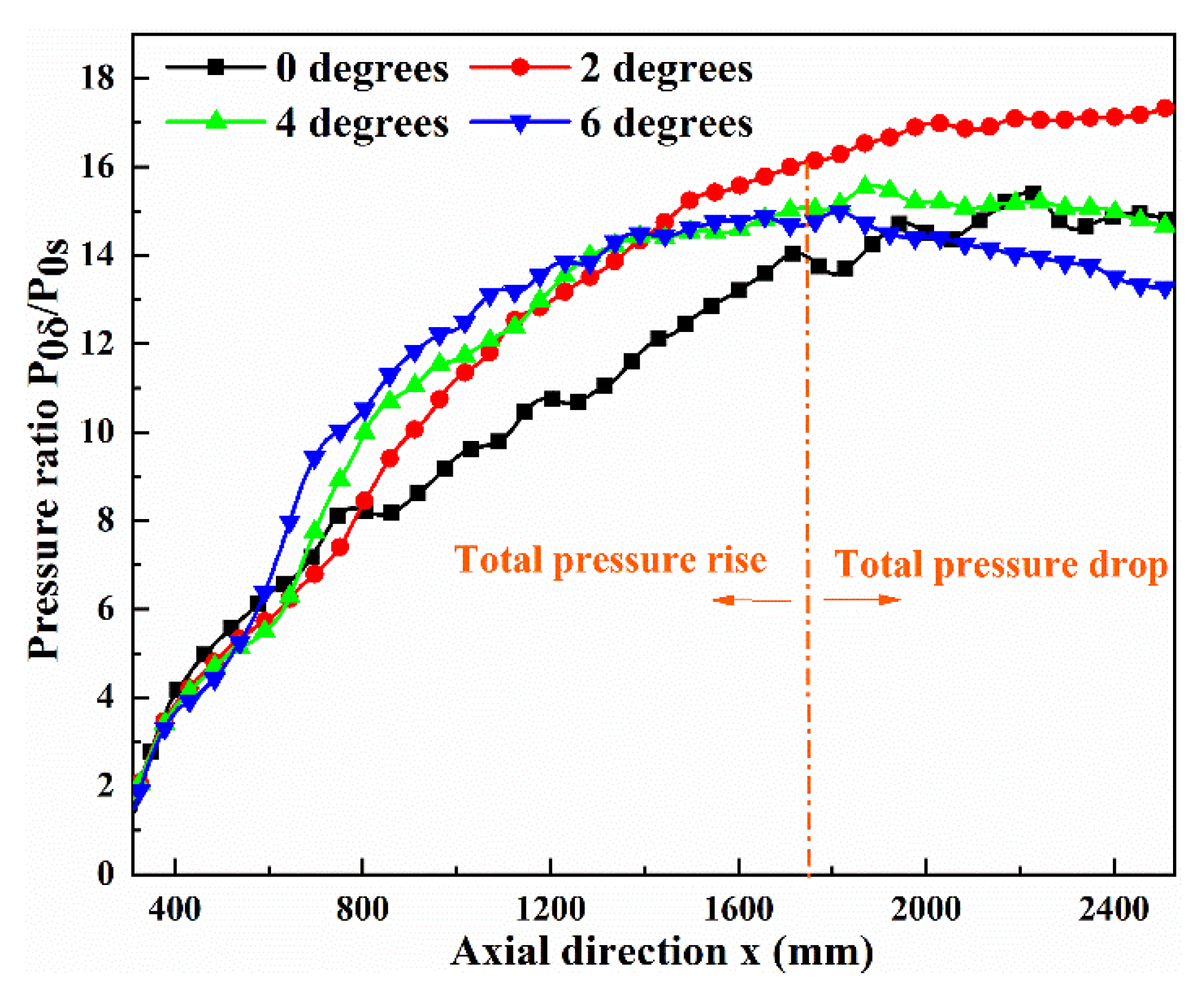
The value of P_0δ/P_0s reflects the pressurization enhancement effect of the primary flow to a certain extent. As in Figure 14, the evolution of the pressurization enhancement (P_0δ/P_0s) along the flow direction in the mixing layer is obtained for different contraction angles. As a result, the pattern of energy variation within the mixing layer can be clearly gained. From that, the pattern of energy variation within the mixing layer can be clearly acquired.

From Figure 14, compared to φ = 0°, the pressurization enhancement within the mixing layer is greater when φ is larger than 0°. P_0δ/P_0s decreases when φ = 4° and 6°, which is different from the later stages of the mixing layer development for φ = 4° and 6°. The main reason is that the pressurization enhancement from the primary flow is already smaller than the pressure loss caused by the wave structure within the mixing layer. Again, it shows that the energy transfer from the primary flow to the mixing layer is also gradually weakening. In the growth phase of P_0δ/P_0s, larger φ leads to larger values of P_0δ/P_0s. On the contrary, in the decreasing phase of P_0δ/P_0s, a larger φ results in a smaller value of P_0δ/P_0s. The reason for that is that the contraction of the mixing chamber promotes the mixing and pressurization of the primary and secondary flows. With further development of flow mixing, a larger mixing chamber contraction angle results in more pressure loss. Thus, the pressurization effect in the later stages of mixing layer development is weakened when φ is larger.

3.3. Performance Variation: Entrainment Ratio and Total Pressure Loss

The development process of the boundary and thickness of the supersonic mixing layer and the pressurization pattern within the mixing layer are described in Section 3.1 and Section 3.2, respectively. Directly responsible for the change in the patterns of supersonic mixing layer development is the variation of φ. Developments in the supersonic mixing layer intrinsically affect the variation of the secondary stream mass flow rate (m_s). Therefore, with the perspective of the supersonic mixing layer, the variation pattern of m_s is explored in this section.

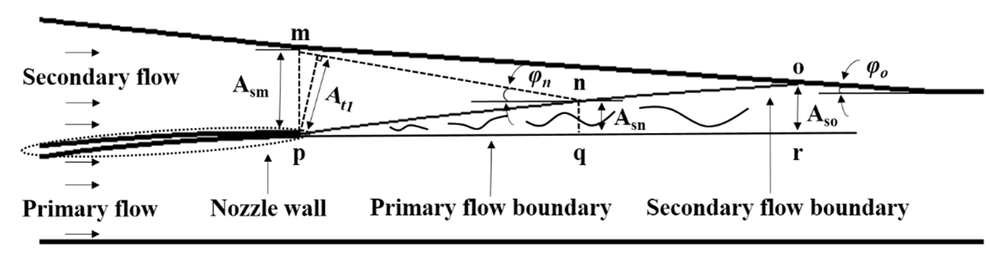
The mixing process of the primary and secondary flows at different contraction angles is depicted in Figure 15. When the contraction angle of the mixing chamber is larger, i.e., φ_n > φ_o, the secondary flow boundary will develop to the wall more quickly. Namely, point n is upstream of point o. Additionally, the non-mixed length l decreases, as shown in Figure 8a. Due to the convective and viscous shear effects of the primary and secondary flows, mass diffusion and transfer take place mainly within the mixing layer. For the high-energy primary flow region, the secondary flow can be neglected for the mass transfer into it. Therefore, the secondary flow passes through the nozzle exit section (m-section) and still develops in a contracting flow channel, i.e., the region of mpqn or mpro. The secondary flow increases in velocity and decreases in static pressure along its path as it develops in the contracted flow channel. The flow mixing area of the secondary flow is smaller when φ is larger, i.e., A_sn < A_so. At this time, the secondary flow channel has a greater shrinkage ratio for a value of A_sm/A_sn larger than A_sm/A_so, resulting in a higher static pressure (Figure 8b) and lower velocity of the secondary flow in the m cross section. Additionally, when φ becomes larger, the minimum circulation area (A_t1) also decreases, resulting in a decline in m_s.

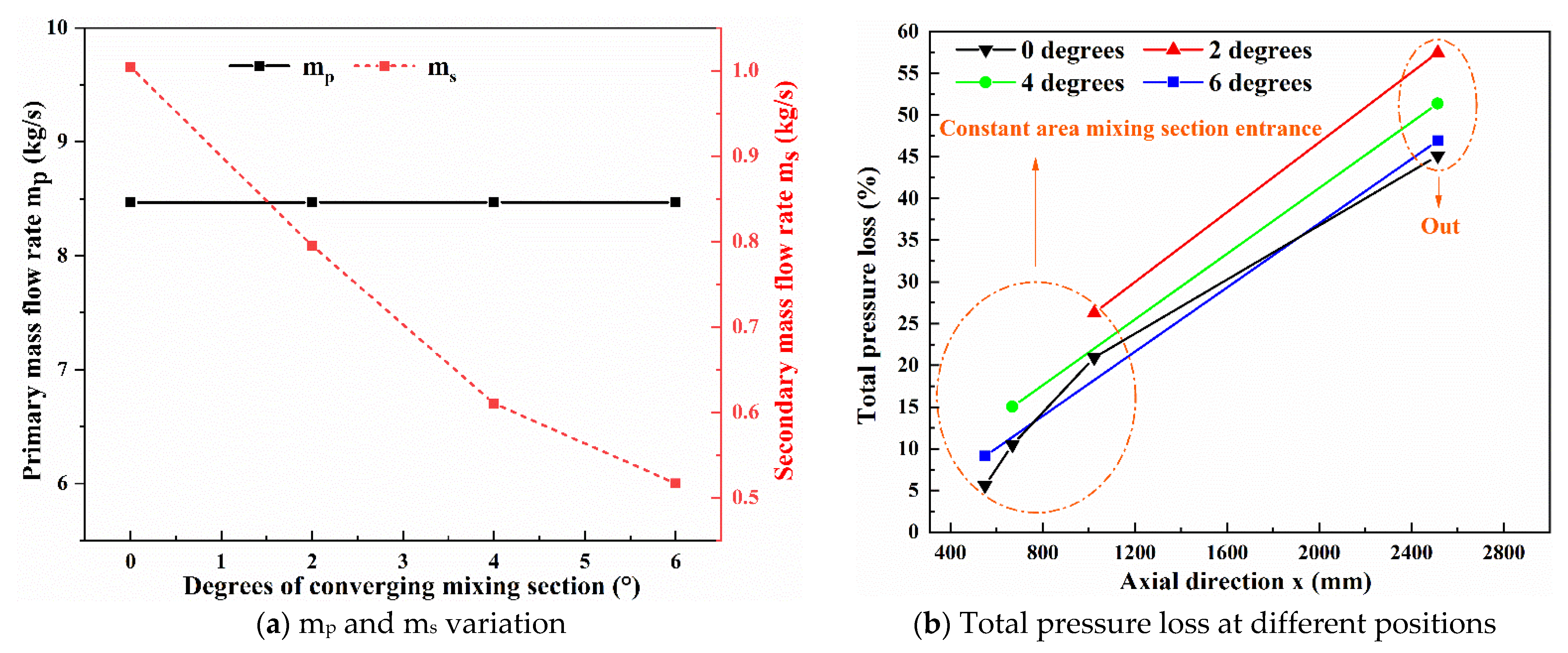
The secondary stream mass flow rate is significantly inhibited by a 35.02% reduction when φ increases from 2° to 6°. However, the primary stream mass flow rate (m_p) is not affected during this process. Consequently, a large mixing chamber contraction angle results in a lower entrainment ratio (ER). The above results can be observed in Figure 16a. The total pressure loss at different locations is depicted in Figure 16b for various φ. As φ increases from 2° to 6°, the mixing chamber length subsequently decreases, and the total pressure loss at the secondary throat inlet gradually falls. At the same time, the total pressure loss at the outlet is also reduced. At the entrance of the secondary throat, the total pressure loss is the largest at φ = 2°, which is 2.89 times of the smallest (φ = 6°). The total pressure loss at the outlet position of the secondary throat is the largest at the mixing chamber contraction angle φ = 2°, with 1.23 times of the smallest (φ = 6°). The presence of contraction produces new oblique shock waves (Figure 13), resulting in additional total pressure loss. Thus, the total pressure loss of the ejector will be greater when the mixing chamber has a contraction angle.

4. Conclusions

The present work focused on investigating the effect of the mixing chamber contraction angle φ on the performance of the central ejector, the development process and the evolution pattern of the mixing layer. Moreover, the central ejector with a mixing chamber contraction angle φ of 0°, 2°, 4° and 6° was set. A comprehensive and detailed analysis was conducted, and the key findings emerged as follows:

(1) The contraction of the mixing chamber has a great influence on the development of the mixing layer boundary. When the contraction angle φ of the mixing chamber gradually increases, the secondary flow boundary develops more easily to the wall, allowing the secondary flow to be covered more quickly. Under the design conditions, the non-mixed length l decreases by 22.12% when the contraction angle φ of the mixing chamber increases from 2° to 6°, and the mixing layer thickness decreases significantly. It can be observed that the non-mixed length l and the mixing layer thickness are negatively correlated.

(2) The secondary flow mass flow rate is reduced by 35.02%, and the total pressure loss at the outlet is reduced by 18.37% when the mixing chamber contraction angle φ = 6° compared to φ = 2°, demonstrating that the non-mixed length l positively correlates with the secondary flow rate. In the range of non-mixed length l, the mixing layer thickness increases in a highly linear manner. After the secondary flow boundary is fully developed to the wall, the mixing layer fluctuates and slowly grows according to the complicated wave structure.

(3) In the early stages of mixing layer development, larger mixing chamber contraction angles result in better pressurization of the secondary flow. However, the P_0δ/P₀₂ will decrease in the later stage of mixing layer development. The reason for this is that the passive pressurization induced by the primary flow is already much less effective than the pressure loss caused by the complicated wave structure.