Article

A Novel Data-Driven-Based Component Map Generation Method for Transient Aero-Engine Performance Adaptation

1
Jiangsu Province Key Laboratory of Aerospace Power System, College of Energy and Power Engineering, Nanjing University of Aeronautics and Astronautics, Nanjing 210016, China
2
AECC Shenyang Engine Design Institute, Shenyang 110066, China
*
Author to whom correspondence should be addressed.
Aerospace 2022, 9(8), 442; https://doi.org/10.3390/aerospace9080442
Submission received: 9 June 2022 / Revised: 29 July 2022 / Accepted: 6 August 2022 / Published: 12 August 2022

Abstract

:
Accurate component maps, which can significantly affect the efficiency, reliability and availability of aero-engines, play a critical role in aero-engine performance simulation. Unfortunately, the information of component maps is insufficient, leading to substantial limitations in practical application, wherein compressors are of particular interest. Here, a data-driven-based compressor map generation approach for transient aero-engine performance adaptation is investigated. A multi-layer perceptron neural network is utilized in simulating the compressor map instead of conventional interpolation schemes, and an adaptive variable learning rate backpropagation (ADVLBP) algorithm is employed to accelerate the convergence and improve the stability in the training process. Aside from that, two different adaptation strategies designed for steady state and transient conditions are implemented to adaptively retrain the compressor network according to measurement deviations until the accuracy requirements are satisfied. The proposed method is integrated into a turbofan component-level model, and simulations reveal that the ADVLBP algorithm has the capability of more rapid convergence compared with conventional training algorithms. In addition, the maximum absolute measurement deviation decreased from 6.35% to 0.44% after steady state adaptation, and excellent agreement between the predictions and benchmark data was obtained after transient adaptation. The results demonstrate the effectiveness and superiority of the proposed component map generation method.

1. Introduction

An Aero-engine is an aerothermodynamic system with strong nonlinearity and advanced technology. The complicated structural designs and rapid dynamic characteristics of aero-engines are crucial in the pursuit of superior performance [1]. Engine designers are faced with various challenges of satisfying growing aero-engine operation and maintenance requirements within the entire flight envelope and life cycle. Hence, a reliable aero-engine mathematic model which can accurately simulate the actual engine behavior is a top priority in aero-engine research [2,3].
The accuracy of an aero-engine mathematic model is strongly dependent on the quality of the component maps, which are generated by implementing rigorous engine rig tests in practice. Among these, compressors are of particular interest because they can cause all sorts of operability problems, such as surges, stalls and fluttering [4], and they can significantly influence the overall performance of aero-engines. Unfortunately, a compressor map is unavailable to ordinary third-party users due to its time-consuming and costly features, which leads to difficulties in its application for aero-engine models. The above limitations motivate researchers to carry out performance adaptation of aero-engine models by modifying or reconstructing compressor maps. According to existing experiment data, the most commonly used method involves tuning the shape of universal maps to reduce engine-to-model mismatches. Stamatis defined a set of scaling factors that represents the degree of deviation between current and optimal key component performance parameters as to-be-adapted parameters during the iterations [5]. In the foundation of this research, Kong distinguished different scaling magnitudes between design and off-design conditions for independent modification based on system identification [6]. Lu introduced an adaptation method based on the aerothermodynamic inverse model to conducting the performance diagnosis [7]. Furthermore, multiple optimization algorithms are applied to search for scaling factors among potential solutions, such as a genetic algorithm (GA) [8], particle swarm optimization (PSO) [9] and quantum PSO [10]. However, the aforementioned research focused on single-point adaptation and neglected the relevance of each off-design condition. Li made a breakthrough in nonlinear multiple-point adaptation [11] which fit quadratic functions to corrected speed curves using scaling factors in off-design conditions. The model predictive capabilities were improved for partial load performances. Despite the extensive advantages and benefits of these modification approaches, the difficulty of tracking with key parameters such as accuracy and local optimum remains a significant impediment to performance adaptation.
Several attempts have been made in a different approach to capture characteristics through data-driven-based methods, owing to their rapid and reliable response [12]. Neural networks (NNs) have been widely used to predict compressor performance [13,14,15]. Ghorbanian investigated a comparison across various NNs in reconstructing axial compressor maps according to rig test data [16,17,18]. Ivanov proposed a computation method for identifying limits by a support vector machine (SVM) and approximating the three-dimensional shape by a response surface method (RSM) of the compressor map [19]. Xu proposed a compressor modeling method by combining two kinds of partial least squares (PLS) with a specific reference value to save computational time and improve accuracy [20]. Tian presented a hybrid model as a linear combination of an NN and PLS to describe the thermodynamic performance of a scroll compressor [21]. Fei introduced a compressor map prediction method using an NN based on the Gaussian kernel function [22]. Another data-driven-based method for performance adaptation directly compensates the performance model output values against the desired values. Volponi presented an enhanced self-tuning on-board real-time model (eSTORM) for aero-engine fault diagnosis [23,24], wherein a series of multi-layer perceptron NNs were adopted to compensate for the measured parameter residuals between the on-board model and actual engine as an empirical model [25]. Ma introduced an adaptive model modification method, estimating a long short-term memory NN representing the initial errors between the performance variations of each turbofan engine within the same fleet [26]. Volponi provided an empirical tuning method for aligning the performance model to an individual engine being monitored to mitigate the effects of engine-to-engine variations [27]. Zhou used Extreme Gradient Boosting (XGBoost) to make the effects of the sequencing on convolution NN adaptation accuracy interpretable, and the method performed well in precision, stability and comprehensibility [28]. Nevertheless, the two major classes of data-driven-based methods above possess separate apparent limitations. The compressor performance prediction method relies on abundant component experiment data, which is costly and time-consuming. Aside from that, the rig test results of an individual component cannot reflect the online operating characteristic concerning the matching and constraint conditions from the upstream and downstream components, having an uncertain and unneglectable influence on the accuracy of the performance model. On the other hand, the direct compensation method is built on measurement. It cannot predict unmeasured parameters, restricting the extended application of the performance model in controller designs and health monitoring.
To address this dilemma, the main contribution of this paper is proposing a novel data-driven-based component map generation method for synthesizing the idea of adaptation. A multi-layer perceptron NN (MLP NN) is utilized to provide key compressor performance parameters, and it is then integrated into a nonlinear component-level model (CLM) of the turbofan engine as an integrated CLM (ICLM). In order to accelerate the convergence and improve the stability in the training process, an adaptive variable learning rate backpropagation (ADVLBP) algorithm is proposed to update the network parameters. Furthermore, this paper creatively adopts unmeasurable state deviations, which represent the deviations between the current and actual component performance parameters, to motivate the retraining of the compressor NN in the adaptation process. According to the measurement deviations between the ICLM and reference engine, two different adaptation strategies which contrapose to steady state and transient conditions are developed to estimate the state deviations, which are used to retrain the compressor MLP NN until the accuracy of the ICLM meets the required target. The advantages of the proposed method include that the quality of the generated MLP NN can be improved through adaptive modification, which is independent of the massive experiment data. Meanwhile, the application of this method is not only restricted to steady state conditions; it also has access to implementing the transient adaptation. The component map reflected by the adapted MLP NN is characterized by certain reasonable principles.
The remainder of this paper is organized as follows. Section 2 presents the methodology. Section 3 introduces the application cases. The corresponding results are demonstrated in Section 4. Section 5 concludes the paper.

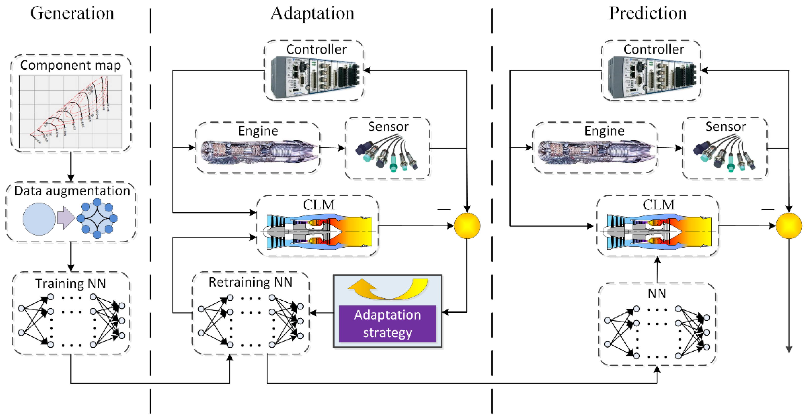
2. Formulation of the Proposed Adaptation Method

2.1. Performance Adaptation

In this section, the formulation of a novel performance adaptation method is introduced to achieve a more accurate CLM for the aero-engine. Due to the particularity of the compressor, the conventional compressor map is replaced by an MLP NN to provide the required key component performance parameters during the gas path calculation. It is widely known that the MLP NN can update the parameters of each neuron according to the gradient descent of the loss function and the chain derivation rule. The loss function is generally constructed from the network output, and the target values are gathered from the test dataset. This paper creatively adopts the deviations between the current and actual component performance parameters to motivate the retraining of the compressor NN. The network can approximate the compressor operating conditions after iterative convergence. However, key component performance parameters cannot be measured directly in practical application, causing difficulty in optimizing the compressor NN parameters adaptively. In order to reconstruct the MLP NN to improve the accuracy of the ICLM offline, a mapping relationship is established between the deviations of the component performance parameters and the deviations of the aero-engine measurable parameters according to corresponding adaptation strategies under steady state and transient conditions. Different adaptation strategies contain multiple approaches for potential problems and requirements, such as network overfitting caused by small sample data and rationality of the shape of speed lines. Finally, such deviations obtained from adaptation strategies can motivate the network to retrain until the measurement deviations are minimized.
In general, any CLM of aero-engines can be simply expressed as follows:
{ x k + 1 = f ( x k , u k ) + w k y k = h ( x k , u k ) + v k ,
where f ( ) denotes the process nonlinear vector function, h ( ) denotes the observation nonlinear vector function, k is the time index, u denotes the control input vector, y denotes the measurable output vector, w and v denote the unrelated process noise and measurement noise, respectively, x denotes the state vector, which represents the component performance parameters, x N 1 and y N 2 .
The framework of the performance adaptation method is shown in Figure 1, including the generation phase, the adaptation phase and the prediction phase. First, a set of characteristic data from existing compressor maps is employed to train the MLP NN after data augmentation. Then, state deviations can be obtained depending on the measurement deviations and adaptation strategies, which are applied to renew the MLP NN parameters. Once the desired accuracy is achieved, the correction process can be terminated. Finally, the adapted MLP NN integrates with the ICLM to implement aero-engine performance prediction.

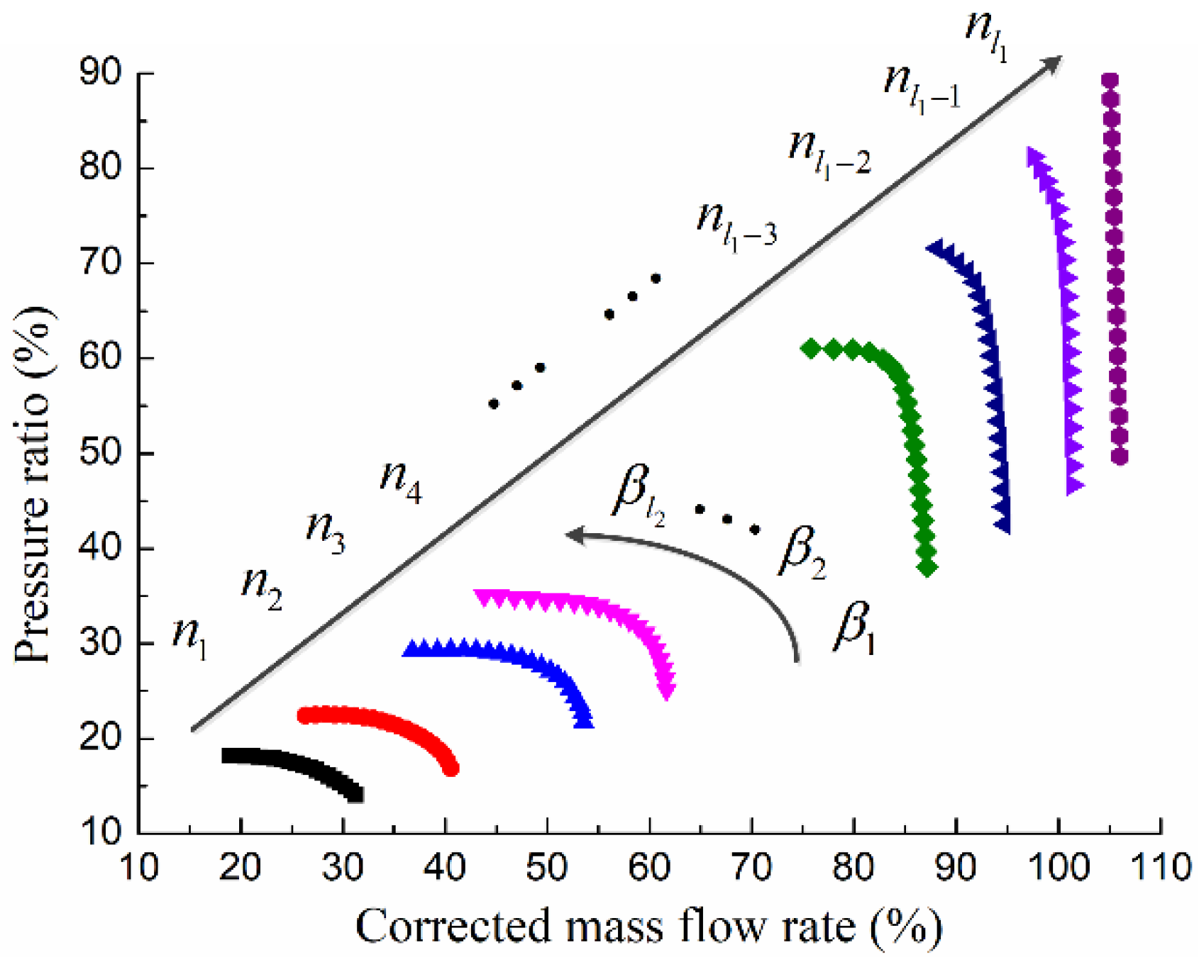
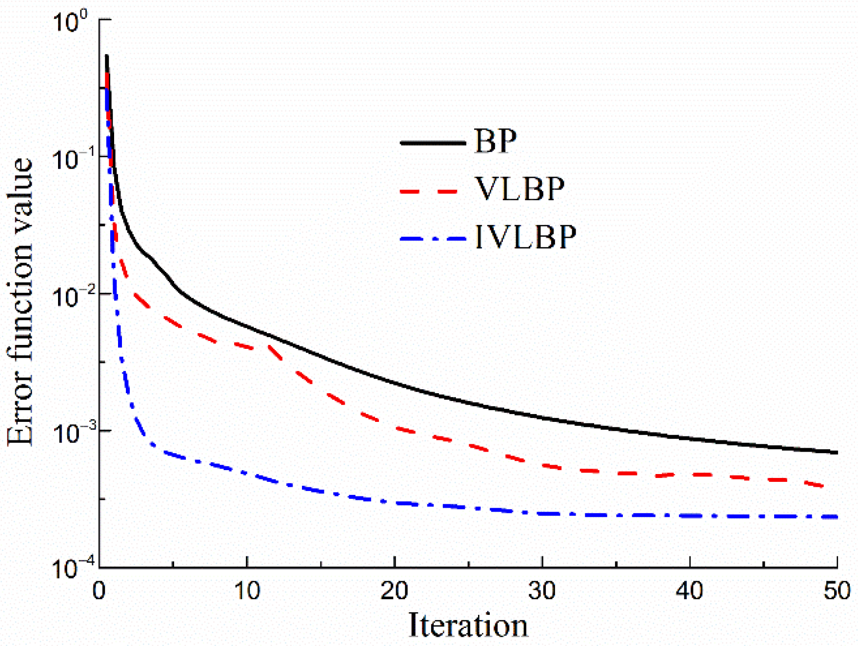
2.2. Compressor Neural Network

A typical map of an axial compressor is schematically illustrated in Figure 2. In the conventional approach, the corrected mass flow rate m ˙ and efficiency η across the compressor are expressed as a function of the pressure ratio π for constant speed lines n . In order to address the non-uniqueness and poor conditioning issues of the compressor map shapes in the conventional interpolation, Kurzke proposed auxiliary coordinates ( β lines) which have no physical meaning [29]. In this situation, m ˙ , π and η can be simultaneously adjusted as the output of the function. An MLP NN is used to establish the mapping relationship in Equation (2), with due consideration to adaptation and prediction. It is worth mentioning that the capacity of time series memory is not required concerning this MLP NN, which represents a regression of the compressor map:
[ m ˙ , π , η ] = Ω ( n , β ) ,
where n = [ n 1 , n 2 , , n l 1 ] T l 1 and β = [ β 1 , β 2 , , β l 2 ] T l 2 are the input vectors of the rotating speed and β lines, respectively, m ˙ ( l 1 × l 2 ) , π ( l 1 × l 2 ) and η ( l 1 × l 2 ) are vectors of the state parameters and l 1 and l 2 are the dimensionality of the training points.
The fundamental calculation process is as follows. For an M - layer NN, the output of the m th layer ( 0 m M 1 ) will act as the input of the ( m + 1 ) th layer:
a m + 1 = ο ( a m ) = g m + 1 ( w m + 1 a m + b m + 1 ) , m = 0 , 1 , , M 1 ,
where a m is the output vector of the m th layer. b m + 1 and w m + 1 are the threshold vector and the weight matrix of the ( m + 1 ) th layer, respectively, g ( ) is the activation function, ο ( ) is the output transfer function, a 0 = [ n , β ] T and a M = [ m ˙ , π , η ] T .
The training algorithm is employed to update the weight and threshold values of the network, minimizing the quadratic error function value J in Equation (4):
J = 1 2 ( t a M ) T ( t a M ) ,
where t is the target output vector.
To accelerate the convergence and improve the stability further in the training process, an adaptive variable learning rate backpropagation (ADVLBP) algorithm is proposed in this paper. Two threshold parameters ( ζ 1 > 0 and ζ 2 < 0 ) are set to evaluate the variation of J . Considering the momentum, the weight increment formula of the m th layer can be expressed as
w k + 1 m = w k m + Δ w k + 1 m
{ Δ w k + 1 m = Δ w k m α k + 1 = α k ρ 1 ,   Δ J k > ζ 1
{ Δ w k + 1 m = μ Δ w k m + α k ( 1 μ ) δ k m ο k m 1 α k + 1 = α k ,   ζ 2 Δ J k ζ 1
{ Δ w k + 1 m = μ Δ w k m + α k ( 1 μ ) δ k m ο k m 1 α k + 1 = α k ρ 2 ,   Δ J k < ζ 2
δ k m = { ο k m ( 1 ο k m ) ( t a k m ) , m = M ο k m ( 1 ο k m ) δ k m + 1 w k + 1 m + 1 , m = 1 , 2 , , M 1
where α is the learning rate, μ is the momentum coefficient, ρ 1 and ρ 2 are the learning rate correction, 0 < μ < 1 , 0 < ρ 1 < 1 , ρ 2 > 1 and Δ J k = J k J k 1 , where J k is the quadratic error function value at time k .
Once J exceeds a minimal pre-set value, the ADVLBP algorithm can be terminated, and the network can predict the compressor performance parameters with high precision.

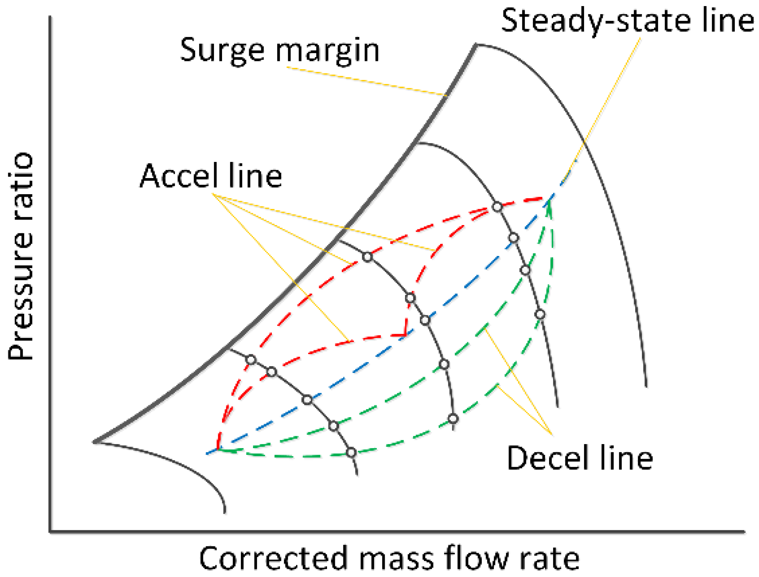
2.3. Steady State Adaptation Strategy

High-quality steady state data are fundamental for adaptation. Due to engine geometry construction restrictions and hostile operating environments, most crucial gas path parameters cannot be measured directly, including the compressor performance parameters [30]. An influence coefficient matrix (ICM) is utilized to obtain state deviations to retrain the compressor NN [31,32]. The idea of the ICM-based method is a linearized model-based inverse calculation. Multiple piecewise linear relationships between the state deviations and measurement deviations can be established in the entire operating conditions of aero-engines. However, a small amount of the steady state benchmark data can cause a destabilized network without reliable application for the ICLM. It is inevitable to implement data augmentation for the MLP NN to ensure the stability and convergency of the ICLM in the iterative computations. Since the aero-engine can approximatively be regarded as a second-order system, massive benchmark datasets are extended to prevent the overfitting of the MLP NN using quadratic polynomials for the rotating speed n according to the existing steady state data.
The ICLM presented with Equation (1) can be expanded in a Taylor series in Equation (10). It is assumed that the higher order term H O T is neglected, and the ambient and control conditions are maintained at the baseline operating points. A linearized relationship can be simplified in Equation (11) between the deviation of the to-be-adapted compressor performance parameters and the deviation of the measured parameters compared with the benchmark datasets. Multiple ICMs are simultaneously established at the entire conditions to improve the accuracy of the linear approximation:
y = y 0 + δ f ( x , u ) δ x | 0 ( x x 0 ) + δ f ( x , u ) δ u | 0 ( u u 0 ) + H O T ,
z y = H ( θ ) ( x x ) ,
where H = ( δ f ( x , u ) / δ x ) | 0 is the ICM, z denotes the measurement from the benchmark datasets, the superscript denotes the benchmark condition of the CLM and θ is the scheduling parameter vector of the ICM. It is assumed that each θ j   ( j = 1 , 2 , , s ) is a real number and ranges between the identical minimum value θ min and the identical maximum value θ max . The corrected rotating speed is selected as the scheduling parameter in this paper, where x N 1 and z N 2 .
Correspondingly, at certain ambient conditions, the state deviations representing the deviation of the to-be-adapted compressor performance parameters can be estimated by inverting the ICM:
x x = H # ( θ ) ( z y )
{ H # ( θ ) = H 1 ( θ ) ,   N 1 = N 2 H # ( θ ) = H T ( θ ) [ H ( θ ) H T ( θ ) ] 1 ,   N 1 > N 2 H # ( θ ) = [ H T ( θ ) H ( θ ) ] 1 H T ( θ ) ,   N 1 < N 2
The state deviations estimated by the ICM-based method are transmitted into the MLP NN directly as the basis of training, and the quadratic error function of the compressor NN in Equation (4) can be revised as follows:
J = 1 2 ( x x ) T ( x x ) = 1 2 [ H # ( θ ) ( z y ) ] T [ H # ( θ ) ( z y ) ]
In this view, Equation (9) can be written compactly as
δ k m = { ο k m ( 1 ο k m ) H # ( θ ) ( z y ) , m = M ο k m ( 1 ο k m ) δ k m + 1 w k + 1 m + 1 , m = 2 , 3 , , M 1
Under steady state operating conditions, a set of benchmark data corresponds to a unique state value and the input value of the MLP NN. Specific values of n and β determine the distribution location of the compressor map, which contains abundant input combinations ( [ n i , β j ] ,   i = 1 , 2 , , l 1 ;   j = 1 , 2 , , l 2 ). If steady state adaptation merely acts on a single input, the parameters nearby the adapted point can be uncontrollable, leading to computational divergence during the iteration of the CLM. Hence, the MLP NN parameters under the input circumstances of all the β j and each n i should be simultaneously adjusted by the same magnitude. The logical relationship can be expressed as shown in Equation (16):
z y x x ( Δ w , Δ b ) ( w , b )
where
( Δ w , Δ b ) = const s .   t .   n i n , β j β
According to the above equations, the measurement deviations actuate the compressor NN parameter update until the ICLM can simulate the actual engine behavior with sufficient accuracy, as can be seen in Figure 3. The proposed steady state adaptation procedure can be briefly described as follows:
Step 1 Data augmentation: According to the existing steady state data, expand the steady state benchmark datasets z using quadratic polynomials.
Step 2 Evaluating measurement deviations z y : Use the current ICLM to carry out the corresponding simulation according to the steady state benchmark datasets z and calculate measurement deviations z y . When the pre-set accuracy requirement is met, go to Step 5; otherwise, go to Step 3.
Step 3 Estimating state deviations x x : Use the ICLM to establish a set of ICMs H ( θ ) and reverse measurement deviations z y to obtain state deviations x x according to Equation (12).
Step 4 Retraining the MLP NN: Use the ADVLBP algorithm to update the compressor NN parameters ( w , b ) to minimize the quadratic error function value J in Equation (14), and then return to Step 2.
Step 5 Store the optimal parameters of the compressor NN.

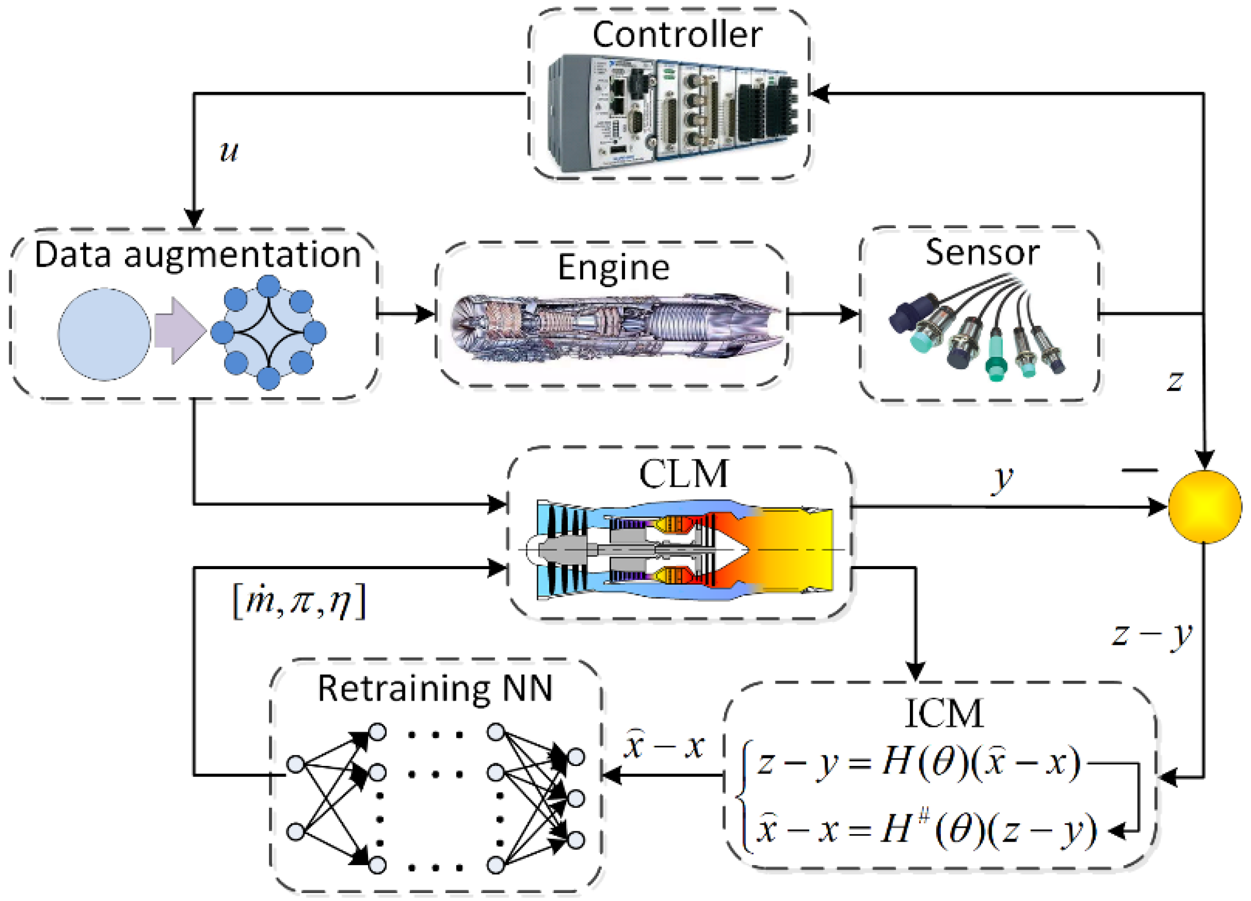
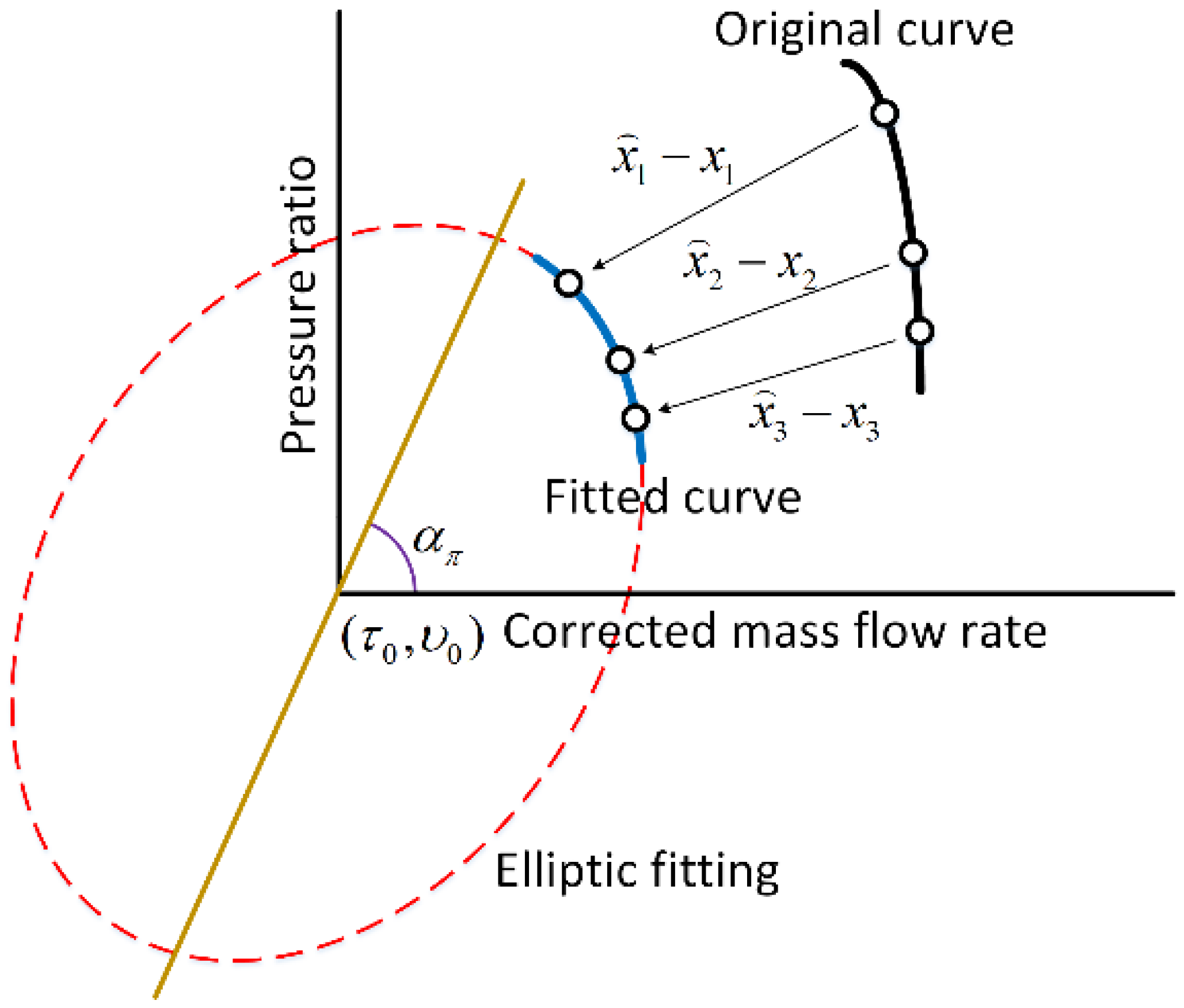
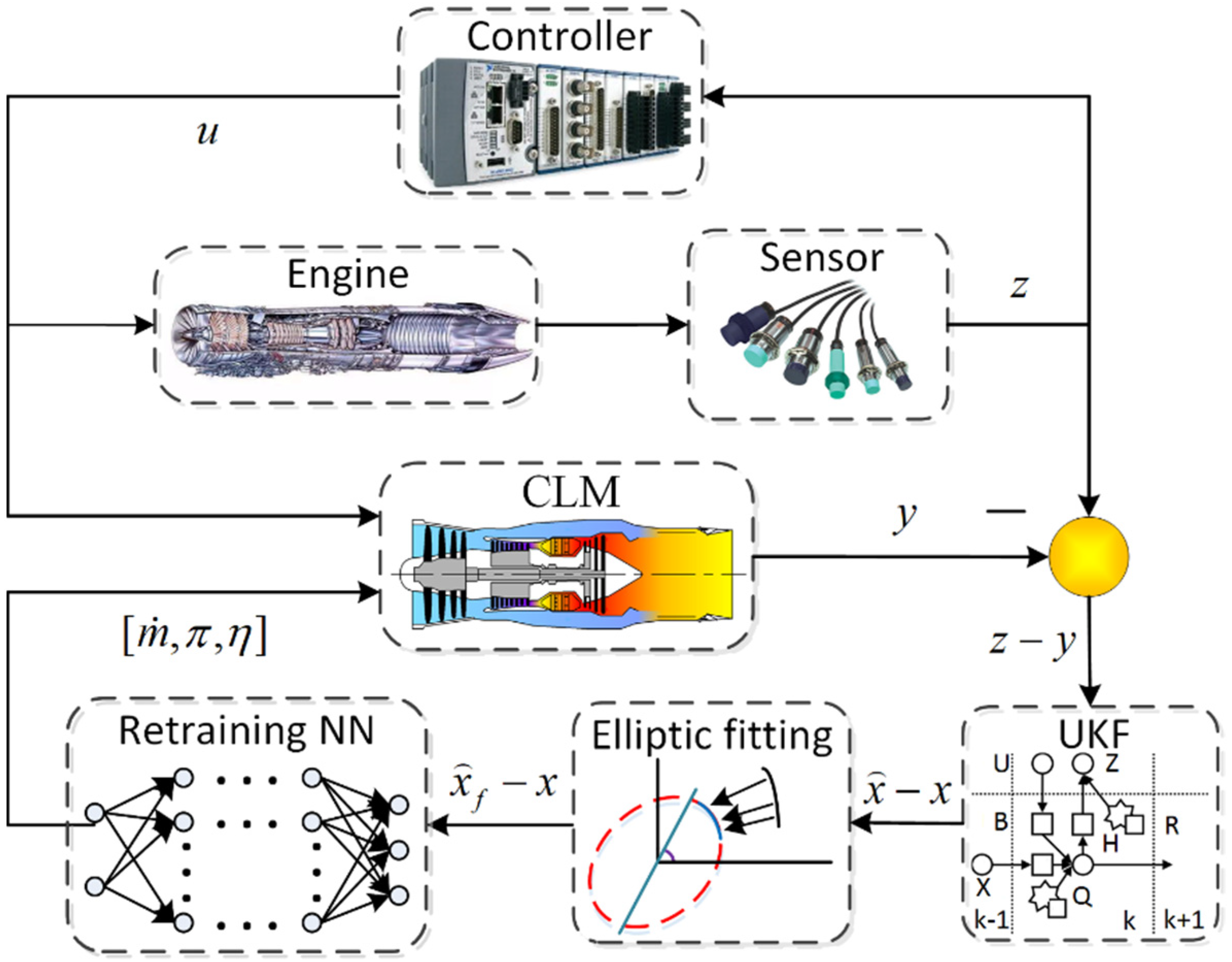
2.4. Transient Adaptation Strategy
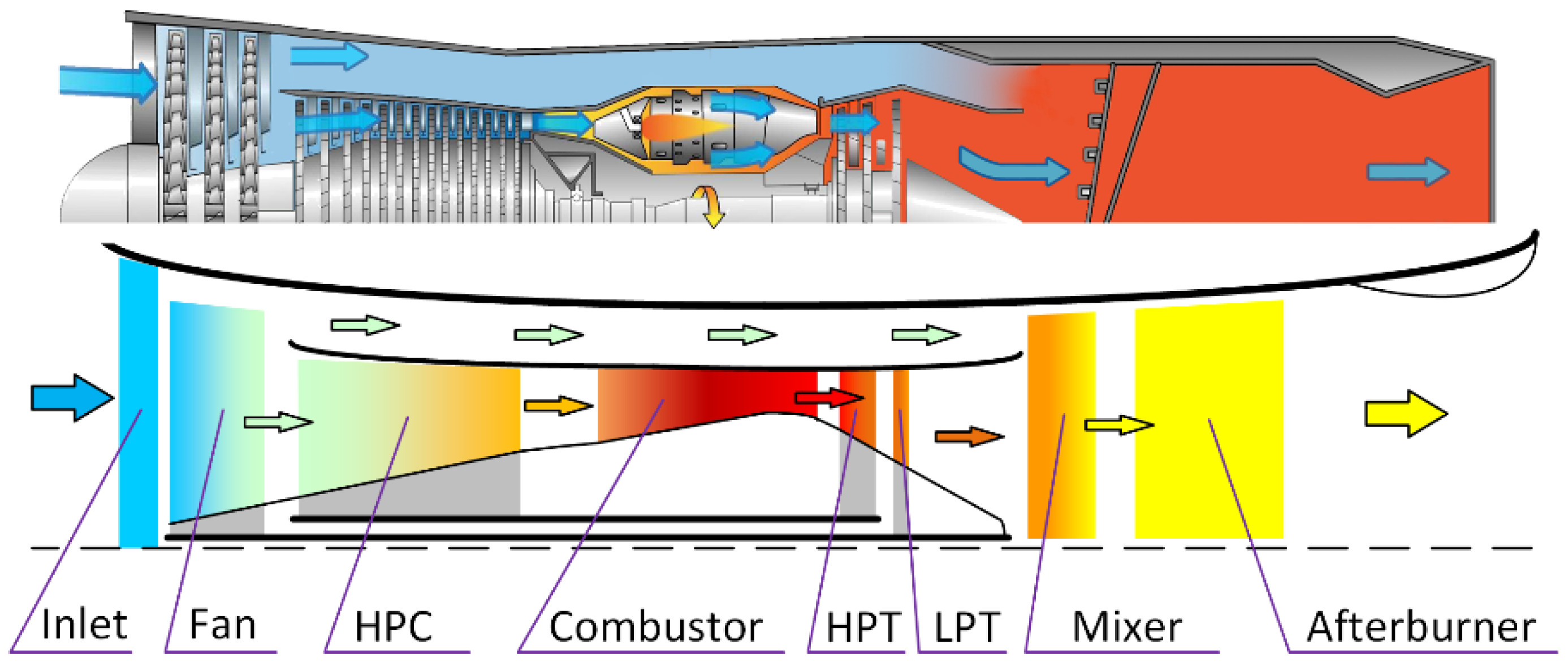
An additional application feature of the proposed method is not only tested for the steady state adaptation, but it also extends the investigation into the transient adaptation.
The proposed steady state adaptation method can develop a high-precision ICLM in a way. However, obtaining high-quality steady state data has proven to be difficult, being time-consuming and expensive [33]. Meanwhile, intensive experiment studies at transient conditions are performed to understand the operating characteristics of aero-engines better. Hence, further research on the transient adaptation strategy is implemented in this section.
In contrast with the steady state adaptation strategy, state deviations under transient conditions cannot be accurately estimated by the ICM-based method due to the noise contamination of the transient benchmark data and the limit that ICM can only be applied to one fixed steady state operating point. To address this issue, the unscented Kalman filter (UKF), with high correction efficiency, strong robustness and a wide application range, is used to approximate the potential solutions [34,35]. This can reflect the nonlinear relationship between the state and measurement deviations, depending on the transient benchmark data. Furthermore, an elliptic fitting method is performed according to the current MLP NN and original state deviations to generate newly fitted curves, which can provide geometric constraints on the shape of the speed lines for transient multipoint correction. Finally, the fitted state deviations can be obtained through comparisons with the current NN output to motivate updating the weight and threshold values of the NN in the new iteration.
A brief description of the UKF filtering process is introduced here. It is assumed that the nonlinear system of aero-engines is provided by Equation (1), in which E ( w k w k T ) = Q k and E ( v k v k T ) = R k . The UKF recursion formula can be expressed as follows.
Step 1 involves filter initialization:
x ^ 0 = E ( x 0 ) ,   P x 0 = E [ ( x 0 x ^ 0 ) ( x 0 x ^ 0 ) T ]
{ W i m = λ / ( r + λ ) W i c = λ / ( r + λ ) + ( 1 ϕ 2 + φ ) , i = 0
W i m = W i c = 1 / 2 ( r + λ ) , i = 1 , 2 , , 2 r
where x ^ 0 and P x 0 are the mean and variance of the initial state, respectively, W m and W c are the weight factors for solving the first-order and second-order characteristics, respectively, λ = ϕ 2 ( r + κ ) r is a scaling factor, ϕ is a zoom factor in regulating the distribution distance of σ points ( 0 < ϕ < 1 ), κ is another zoom factor, φ denotes the information of the state distribution, φ = 2 for the Gaussian system generally and r is the dimension of the state vector.
Step 2 is calculation of the σ point:
χ k 1 = [ x ^ k 1   x ^ k 1 + ( r + λ ) P x k 1   x ^ k 1 ( r + λ ) P x k 1 ]
where the subscript k 1 indicates the last sampling step.
Step 3 is a time update:
{ χ i , k | k 1 = f ( χ i , k 1 , u k ) x ^ k | k 1 = i = 0 2 r W i m χ i , k | k 1 P x k | k 1 = i = 0 2 r W i c ( χ i , k | k 1 x ^ k | k 1 ) ( χ i , k | k 1 x ^ k | k 1 ) T + Q k 1 γ i , k | k 1 = f ( χ i , k | k 1 , u k 1 ) y ^ k | k 1 = i = 0 2 r W i m γ i , k | k 1
where χ and γ are the values of the σ points transferred from the process function and observation function, respectively. The subscript k | k 1 indicates the information at time k based on the information available up to and including time k 1 . Finally, P x k | k 1 is the forecast error covariance.
Step 4 involves updating the measurement:
{ P y k = i = 0 2 r W i c ( γ i , k | k 1 y ^ k | k 1 ) ( γ i , k | k 1 y ^ k | k 1 ) T + R k P x k y k = i = 0 2 r W i c ( χ i , k | k 1 x ^ k | k 1 ) ( χ i , k | k 1 x ^ k | k 1 ) T K k = P x k y k P y k 1 x ^ k = x ^ k | k 1 + K k ( z k y ^ k | k 1 ) P x k = P x k | k 1 K k P y k K k T
where P x k y k is the cross covariance, P y k is the innovation covariance, K k is the Kalman gain matrix, x ^ k is the state estimation and P x k is the data assimilation error covariance.
After the UKF estimation is completed, the following objective is to retrain the compressor NN. It is worth emphasizing that the locations of the transient operating points distributed in the component map at the same corrected rotating speed can be diverse, which can be seen in Figure 4. The excess power of aero-engines can broadly impact the integrated dynamic property, leading to the magnitudes of the acceleration and deceleration rates. Therefore, the correction of each β at the same speed line needs to be variational. A nonlinear component map elliptic fitting method is applied to analytically construct relationships among the key compressor parameters and replace conventional lookup tables in an aero-engine model configuration [36,37]. The equation, adjusted for the m ˙ versus π map, is given by
( m ˙ 0 τ 0 a π ) 2 + ( π 0 υ 0 b π ) 2 = 1
where a π and b π are the semi-major and semi-minor axes of the ellipse, respectively, and m ˙ 0 and π 0 represent the corrected mass flow rate and pressure ratio in the fitted component map, respectively, which centers at ( τ 0 , υ 0 ) by elliptic fitting. In addition, the capacity to rotate freely from the ellipse is considered to increase the degrees of freedom in map tuning such that m ˙ versus π can be obtained by
[ m ˙ π ] = [ cos ( α π ) sin ( α π ) sin ( α π ) cos ( α π ) ] [ m ˙ 0 π 0 ] ,   Φ ( α π ) = [ cos ( α π ) sin ( α π ) sin ( α π ) cos ( α π ) ]
where α π is the angle of the ellipse to rotate and Φ is the rotational coefficient matrix. The application of this elliptic fitting method for the selected map is shown in Figure 5, where x i x i   ( i = 1 , 2 , 3 ) is the fitted state deviation of each operating point. The key component parameters are modified using original state deviations estimated from the UKF. The calculation procedure of m ˙ versus η is closely analogous to that expressed in Equations (24) and (25) such that it cannot be covered again here. The logical relationship of the transient adaptation strategy can be expressed by
z y x x x f x ( Δ w , Δ b ) ( w , b )
where subscript f denotes the fitted parameters.
The magnitude of the modification of the scaled map depends on the sub-coefficients of the elliptic fitting method, simultaneously ensuring the rationality of the map shape and nonlinear multipoint correction at the same speed line, and the ICLM after adaptation can provide accurate matching to the actual engine under transient conditions. The proposed transient adaptation method, which is illustrated in Figure 6, can be briefly described as follows:
Step 1 Evaluating measurement deviations z y : The current ICLM is used to carry out the corresponding simulation according to a set of transient benchmark data z containing measurement noise and uncertainty, and measurement deviations z y can be obtained as an evaluation index. Once the pre-set accuracy requirement is met, proceed to Step 5; otherwise, proceed to Step 2.
Step 2 Estimating original state deviations x x : The UKF expressed in Equations (18)–(23) is utilized to estimate original state deviations x x according to measurement deviations z y .
Step 3 State transition: The fitted points are the superposition of the points at the current component map and original state deviations x x . On top of this foundation, a nonlinear elliptic fitting method expressed in Equations (24) and (25) is employed to reconstruct the shape of the map curves, and fitted state deviations x f x , corresponding to all β at the same fitted speed lines, can be determined.
Step 4 Retraining the MLP NN: The ADVLBP algorithm is used to retrain the compressor NN according to fitted state deviations x f x . Then, return to Step 1.
Step 5 Store the optimal parameters of the compressor NN.

3. Application

The objective of this research is a twin-spool turbofan engine, which is widely used in aerospace applications. The configuration of the turbofan engine is illustrated in Figure 7. The typical components of the engine contain an inlet, a fan, a high-pressure compressor (HPC), a combustor, a high-pressure turbine (HPT), a low-pressure turbine (LPT), a mixer, a bypass, an afterburner and a nozzle.
Since the primary target of this paper is to assess the effectiveness of the proposed adaptation method, the quality of the measurements is crucial for the above purpose. The selected measurable parameters under a Gaussian white noise environment for performance adaptation simulation are listed in Table 1. The measurable output vector of the nonlinear system described in Equation (1) is given by
y = [ n L , n H , T t 25 , P t 3 , P t 6 , T t 6 ] T 6
The CLM is established based on the previous work [38] by a set of mathematical formulas for aero-engines according to the principles of aerothermodynamics, rotor dynamics and other principles followed by various engine components. The gas path parameters can be calculated by adopting a series of physically based empirical formulas under a few assumptions. An MLP NN is substituted for the universal compressor map that is available from the gas turbine performance simulation software GasTurb, providing indispensable compressor performance parameters in the iterative procedure of the ICLM. In addition, relatively small amounts of data from the compressor map are insufficient to support the training of the MLP NN. It is inevitable to expand the data by interpolation and extrapolation schemes [39]. The state vector of the nonlinear system can be described in Equation (1). However, due to the copyright protection and expensive cost of the experiment data, a reference engine is a traditional CLM using another different compressor map implemented as a lookup table to generate steady state and transient benchmark data:
x = [ m ˙ , π , η ] T 3
Three cases, Cases 1–3, are created to test the developed adaptation method. The first case study assesses the convergence ability of the ADVLBP algorithm in the training phase. The training dataset comes from a source of a universal compressor map in GasTurb. On the other hand, the objectives of Case 2 and Case 3 are to directly evaluate the combined accuracy and optimization procedure in the adaptation phase under the steady state and transient conditions of aero-engines, respectively. Case 2 and Case 3 verify the capacity of adaptation of the ICLM by corresponding adaptation strategies. The multipoint steady state fuel flow rate is scheduled in Case 2, and the fuel flow rate varies according to the controller following the rotating speed command schedule in Case 3. In addition, the transient simulation of Case 3 considers random noise contamination, which can closely simulate the actual operating environment.

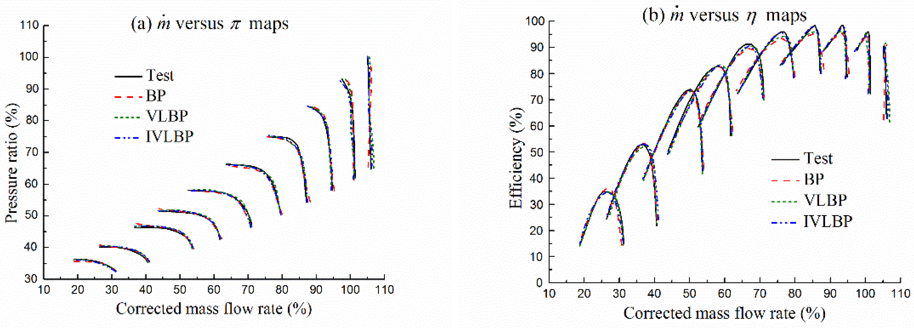
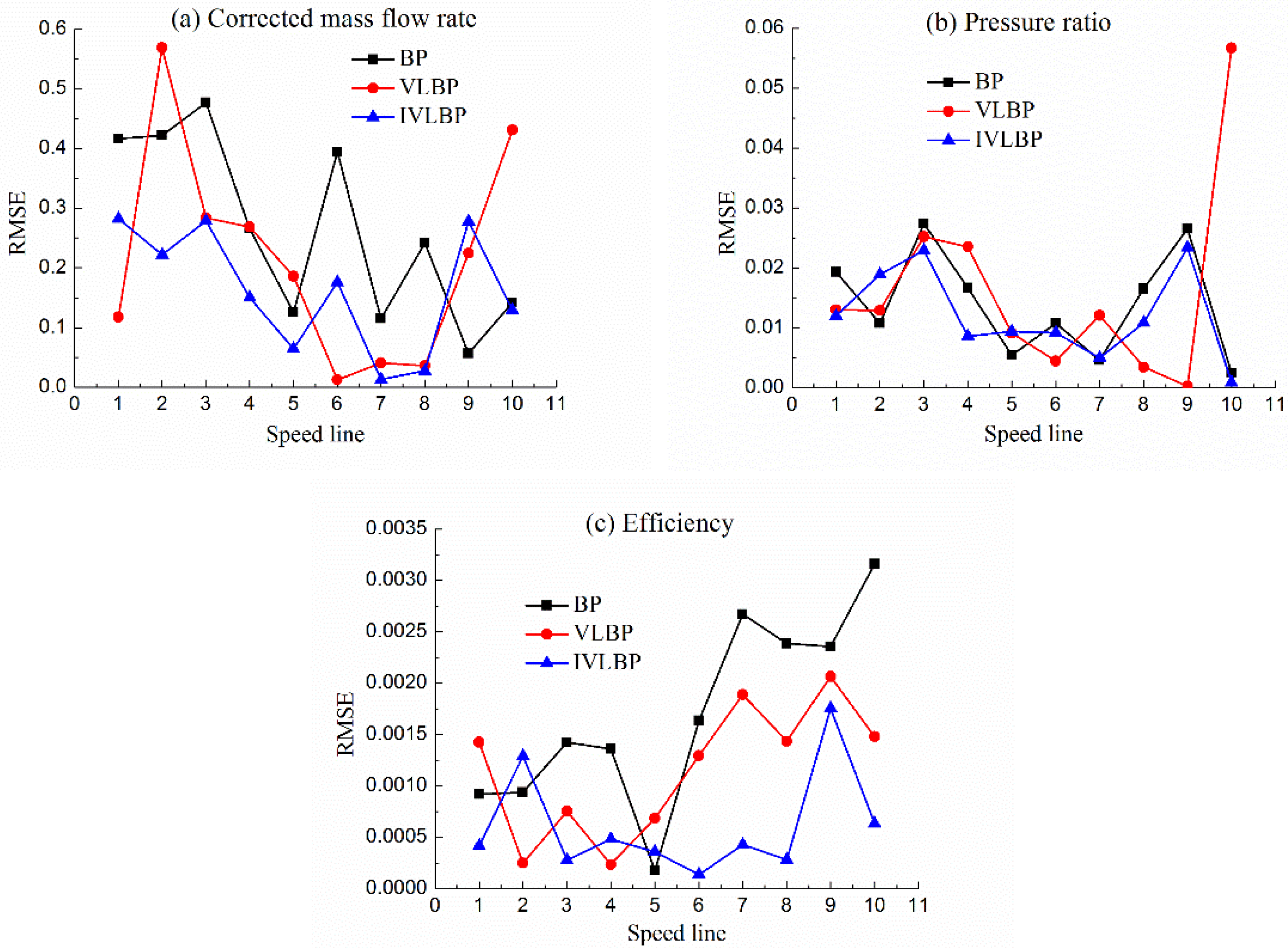
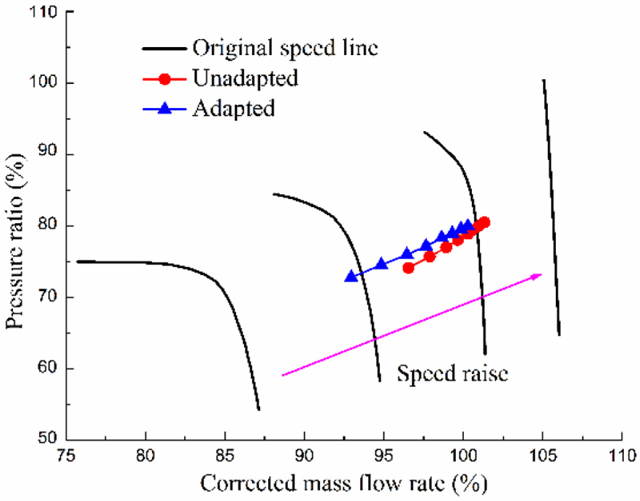
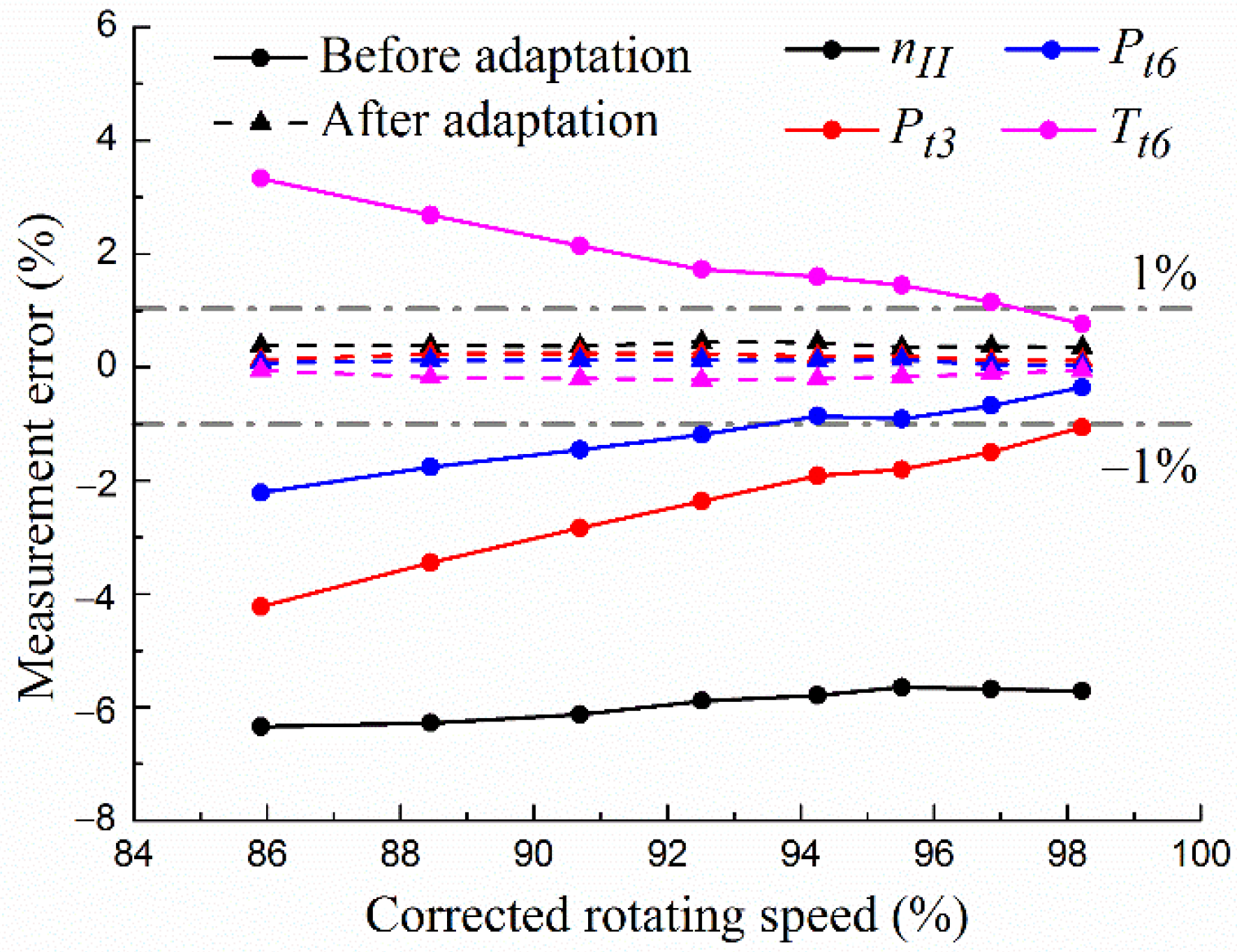
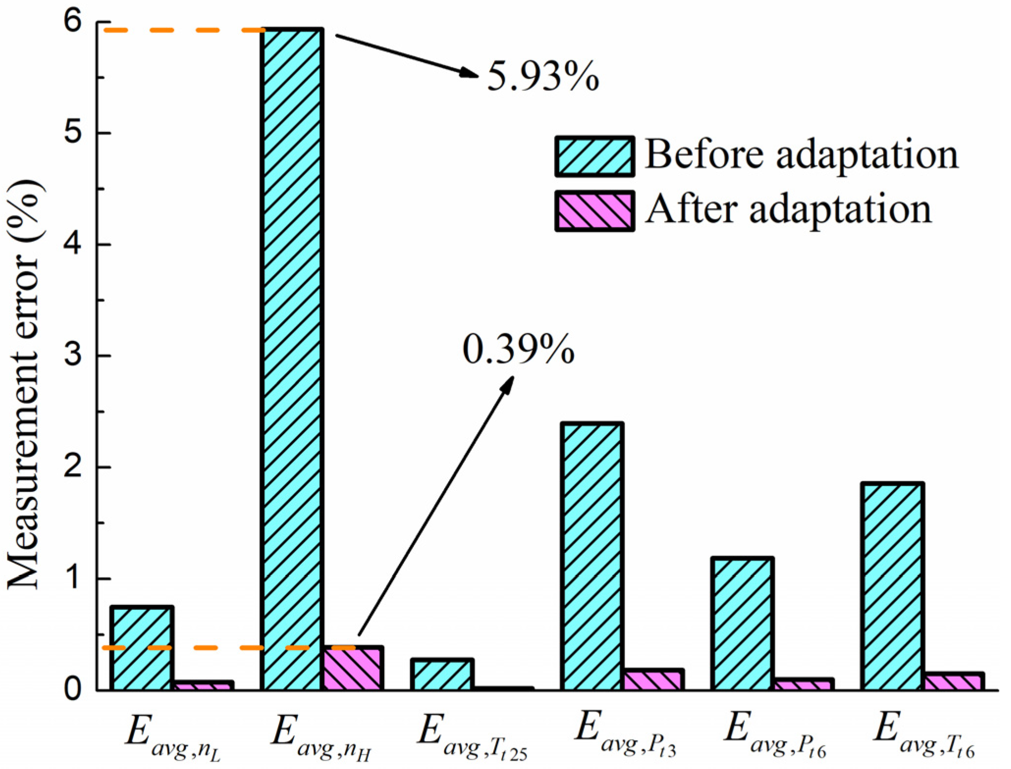
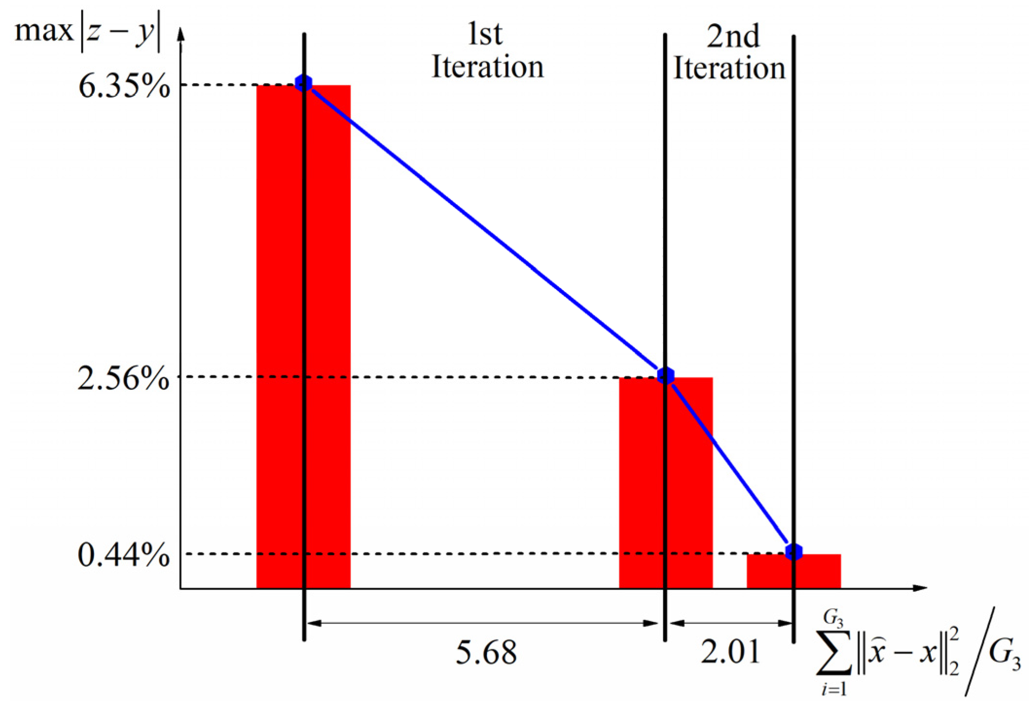
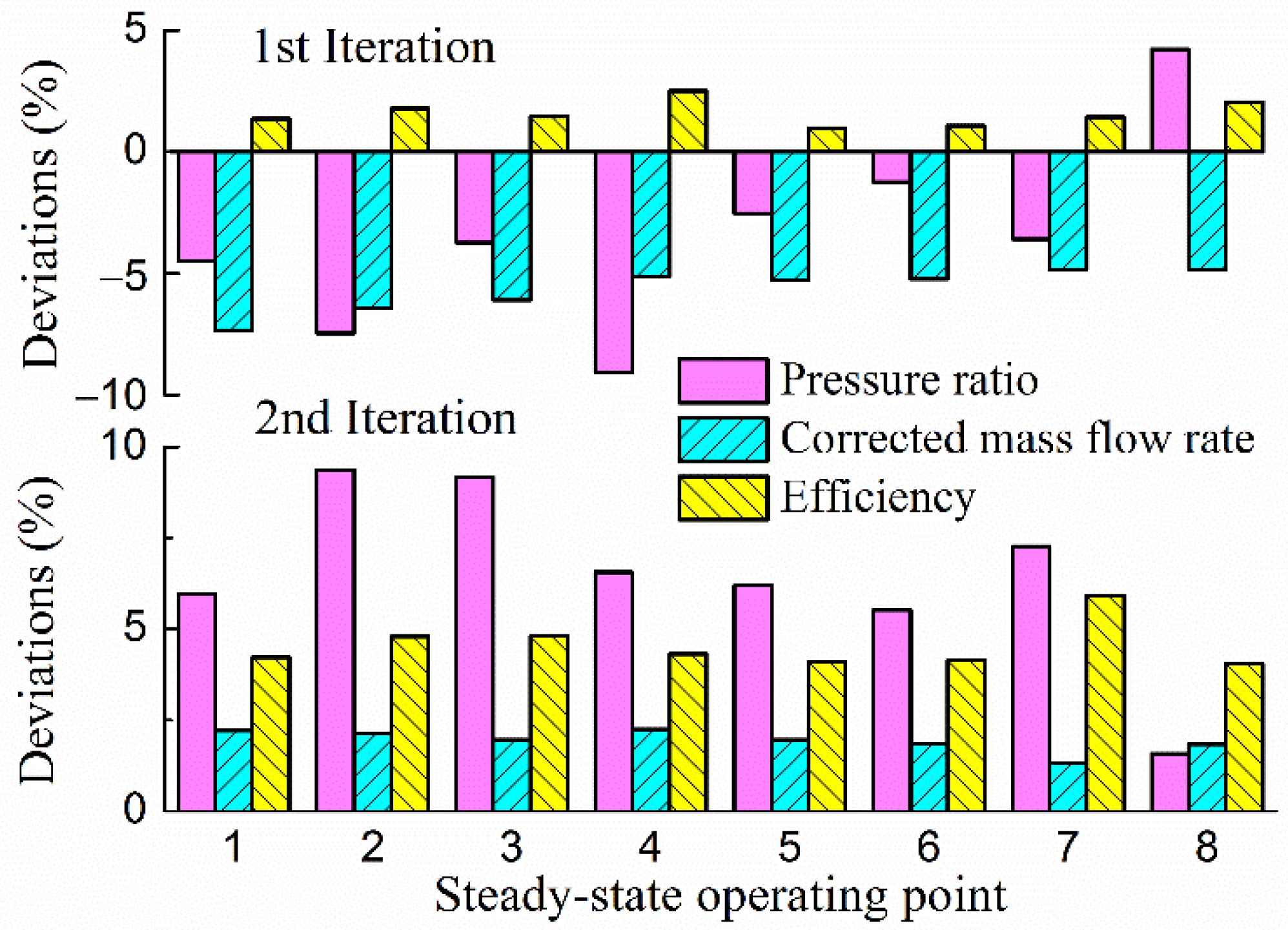
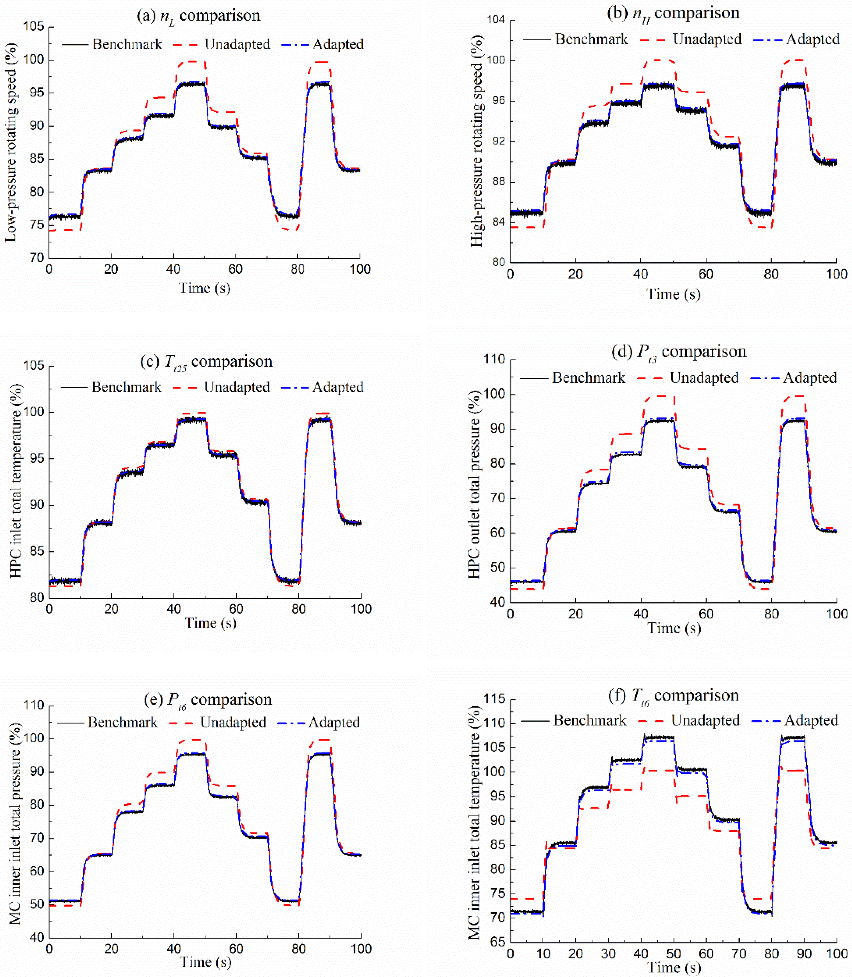
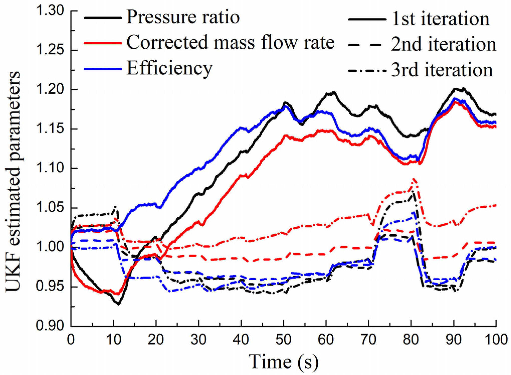
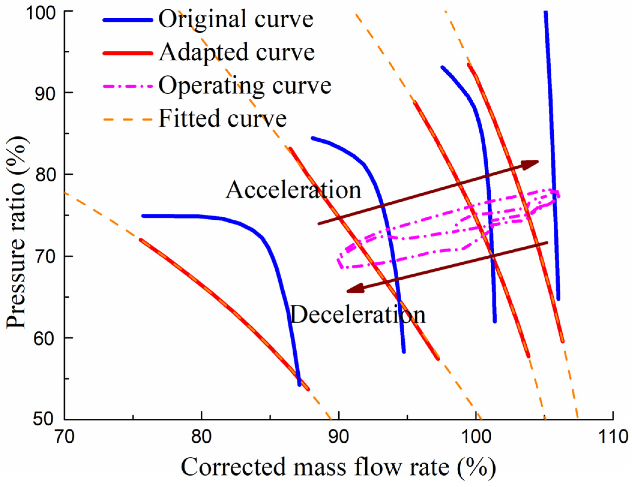
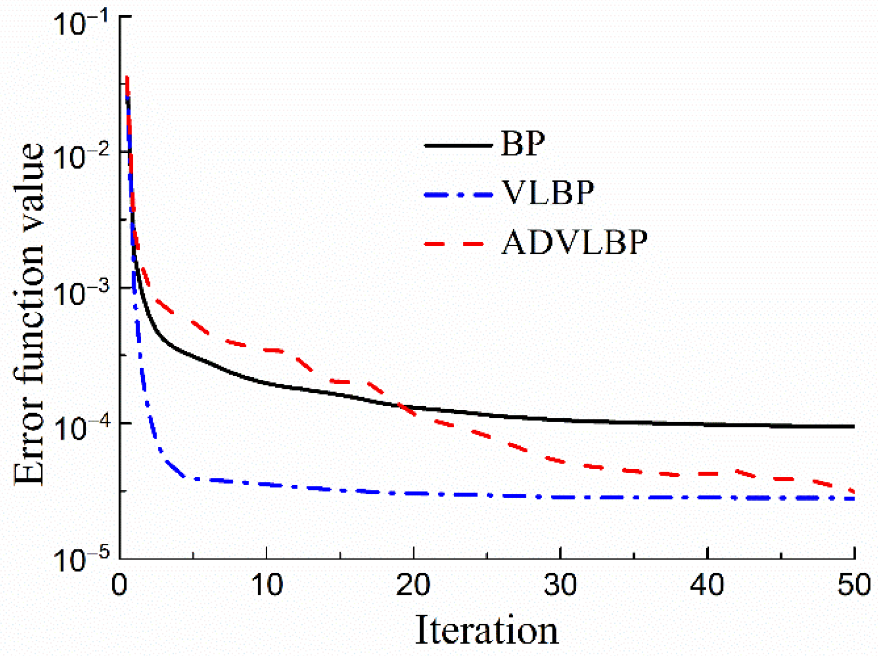
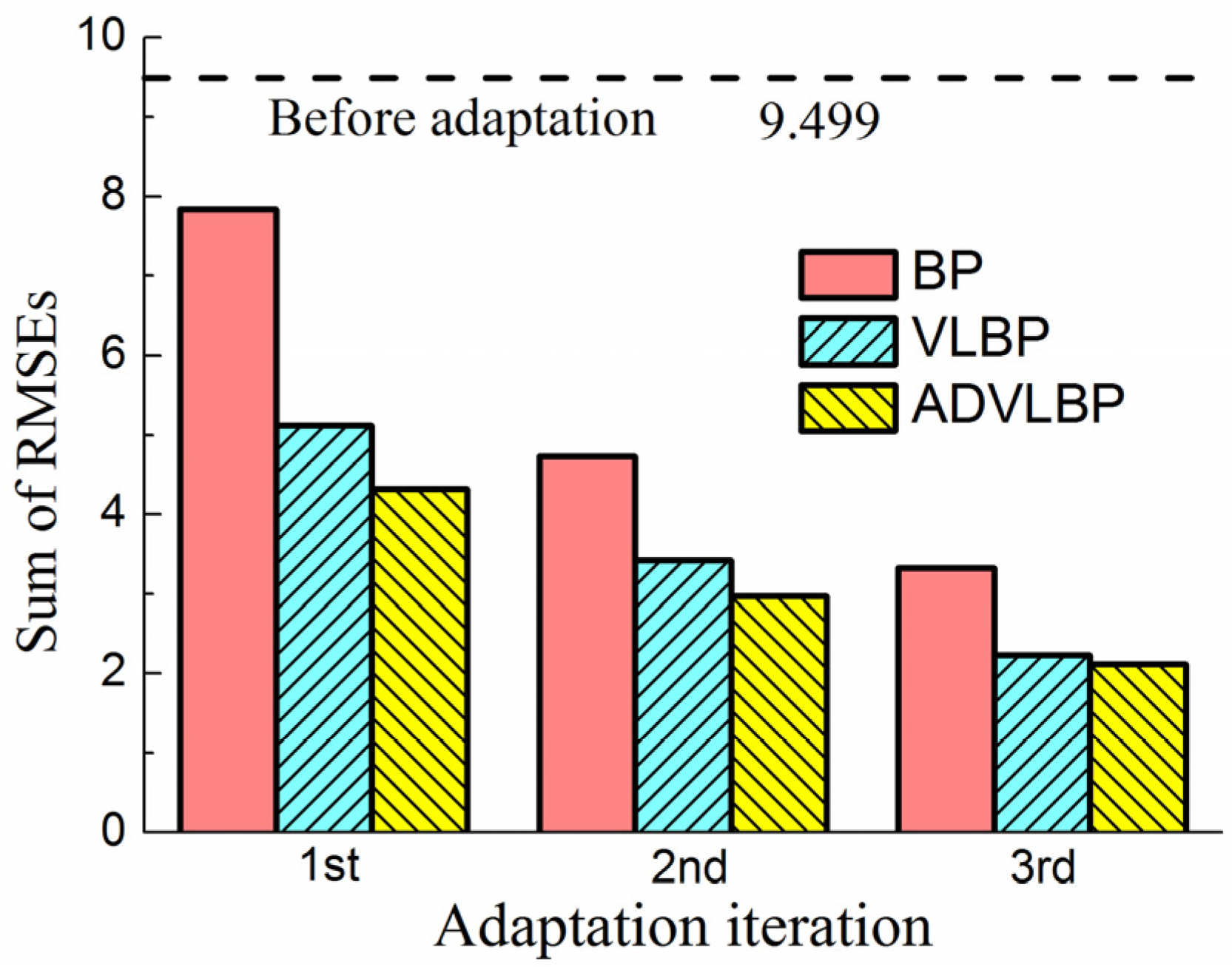
4. Results and Discussion
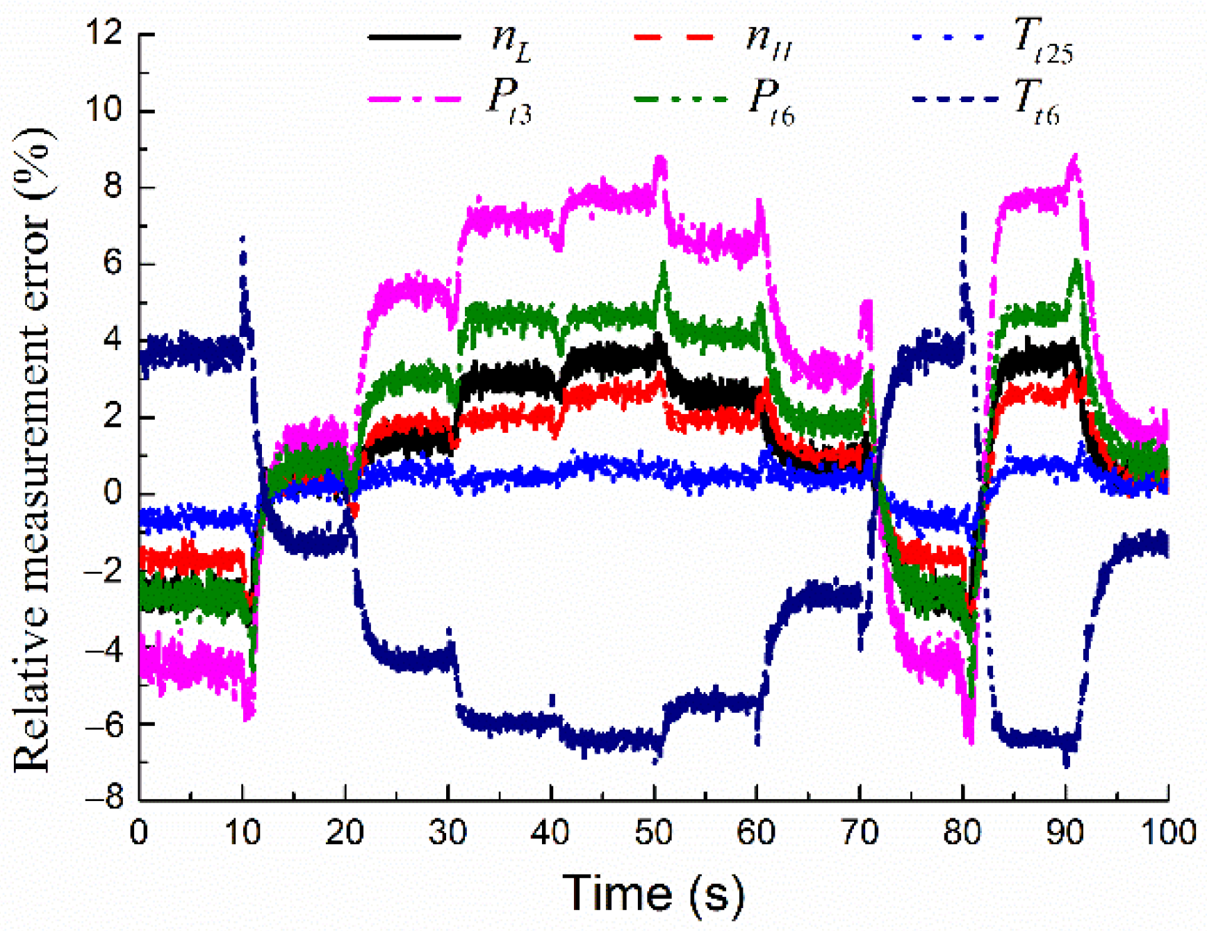
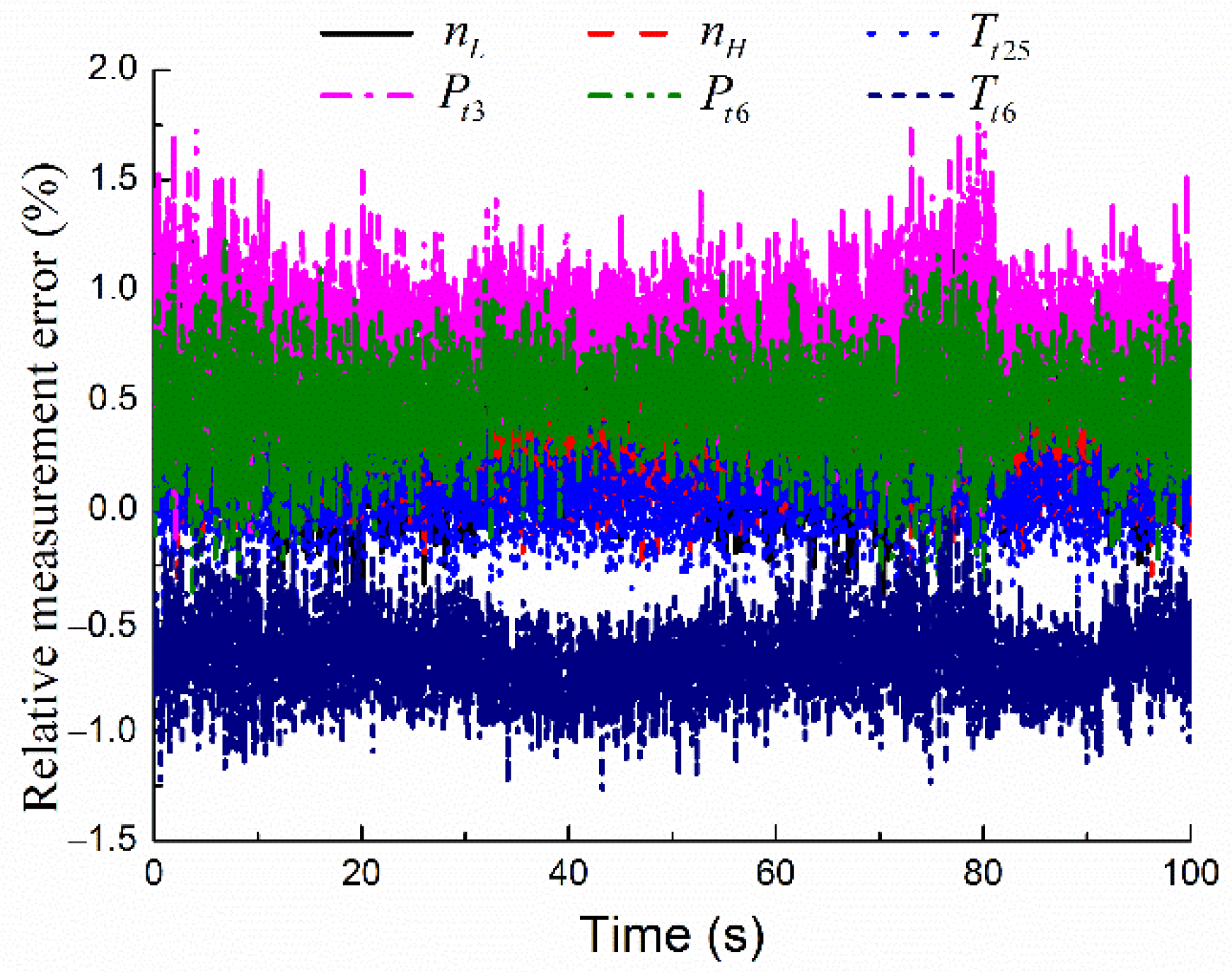
4.1. Case 1

As previously introduced, Case 1 simulates the corrected mass flow rate, pressure ratio and efficiency as a function of β and the corrected rotating speed for a compressor NN. In the conventional approach, the compressor map is illustrated as a distribution of discrete points, and the volume of data is relatively small. Due to the overfitting of the MLP NN under the circumstances of small sample tasks, data augmentation is utilized to expand the training datasets, and interpolation and extrapolation schemes are employed to determine the unknown values at desired positions.
A total of 200 sets of the compressor map data from GasTurb was selected as the training dataset. The data augmentation was carried out according to the following rules: the auxiliary parameter β varied from −1.1 to 1.1 with an increment of 0.001, and the corrected rotating speed n varied from 0.4 to 1.1 with an increment of 0.001. More than 800,000 sets of training data were obtained, following linear interpolation and extrapolation principles. To avoid poorly conditioned network parameters and accelerate the convergence of the MLP NN, normalization of the data needed to be performed before training.
The determination of the network structure parameters was high on the list of priorities. The improper number of hidden layers and neuron nodes could lead to divergency, inaccuracy and overfitting of the MLP NN. After empirical adjustment, the MLP NN employed in this paper contained an input layer, two hidden layers and an output layer. It had two neurons in the input layer corresponding to two inputs (n and β). The numbers of the hidden layer nodes were nine and seven, respectively. Finally, the network had three neurons in the output layer, representing the state vector x.
To demonstrate that the ADVLBP algorithm could obtain higher accuracy and faster convergence compared with the pure backpropagation (BP) [40] and variable learning rate backpropagation (VLBP) [41] algorithms with the same quality and quantity training data, a series of initial weight and threshold values of the MLP NN was generated equally for the testing of the three algorithms. The parameters of the algorithm were set as follows: ζ1 = 0.05, ζ2 = −0.5, ρ1 = 0.75 and ρ2 = 1.05. Under the circumstances of the same number of iterations, which was 50, the simulated quadratic error function values of the three algorithms are compared in Figure 8. As shown in Figure 8, the ADVLBP algorithm had an obvious smoother and faster convergence procedure than the other two algorithms under the same parameter settings and performance function. This indicates that the ADVLBP algorithm is more sensitive to the region in which the surface of the error gradient varies, which can more strikingly achieve the learning purpose.
A further investigation was performed for the prediction accuracy of the MLP NN. Figure 9 illustrates the results for the BP, VLBP and ADVLBP algorithms. It can be seen in Figure 9 that the values at all speed lines estimated by each of the above three MLP NNs were in good agreement with the test data, and the visual locations of them were distinguished inconspicuously. It may be concluded that all the MLP NNs were able to model the characteristic curves. That aside, a careful inspection of Figure 9 reveals that the prediction differences of the MLP NNs based on the BP, VLBP and ADVLBP algorithms at each speed line were evident in quantitative terms according to the root mean square error (RMSE) provided in Equation (29):
E R M S E = 1 G 1 i = 1 G 1 ( x i x i ) 2
where G 1 is the number of the test data at each speed line and x and x are the test and estimated state vectors, respectively.
Figure 10 presents the predicted RMSE of the MLP NNs using the BP, VLBP and ADVLBP algorithms at each speed line. From the figure, the blue lines are distributed underneath the other two lines in general, which shows that the ADVLBP-based NN had a more acceptable prediction accuracy than the other two NNs. Otherwise, the maximum values of the RMSE of m ˙ based on the BP, VLBP and ADVLBP algorithms were 0.477, 0.569 and 0.282, respectively, the maximum values of the RMSE of π based on the BP, VLBP and ADVLBP algorithms were 0.027, 0.058 and 0.023, respectively, and the maximum values of the RMSE of η based on the BP, VLBP and ADVLBP algorithms were 0.003, 0.002 and 0.001, respectively. In summary, the proposed MLP NN in this paper can accurately reflect the compressor performance in different situations, which has the capability of rapid convergence.

4.2. Case 2

The objective of the second case was to test the accuracy of the proposed adaptation method in steady state conditions, and state deviations were obtained using the steady state adaptation strategy according to measurement deviations in the premise of data augmentation. Multiple off-design points were used to verify the matching degree between the ICLM and the reference engine.
In the international standard atmosphere (ISA) conditions, a series of simulations of the ICLM before and after adaptation were performed compared with the steady state benchmark data. The eight operating points were arranged in sequence from the high to low conditions of the aero-engine. Point 8 of the original model had the worst accuracy concerning the relatively lowest state, which can be seen in Figure 11 and Figure 12. It is observed in Figure 12 that the ICLM cannot simulate the performance of the reference engine at an appropriate level of accuracy before any retraining of the compressor NN is employed. Substantial improvements in performance accuracy occurred after the adaptation. The maximum absolute error decreased from 6.35% to 0.44%. To make the results more intuitive, Figure 12 shows the absolute errors of n H , P t 3 , P t 6 and T t 6 , which exceeded 1%. All measured parameters for the adapted ICLM presented an absolute error in the range from −0.5% to 0.5%.
Moreover, in order to better evaluate the overall quality of the proposed adaptation method, the average measurement deviation is introduced in Equation (30), and the corresponding simulation is presented in Figure 13. The blue and purple bars represent the unadapted and adapted CLMs, respectively. An apparent reduction in magnitude can be seen, and the maximum average measurement deviation decreased from 5.93% to 0.39%. Figure 14 presents the iterative convergence procedure of the steady state adaptation method based on the ICM. As shown in Figure 14, the prediction accuracy was improved with the increasing iteration. Among them, the ordinate represents the maximum measurement deviations, and the abscissa represents the average 2-norm of the state deviations, where G 3 denotes the number of steady state benchmark datasets. It declares that the prediction accuracy sharply improved with a rapid linear approximation, and the adapted ICLM met the expected requirements through only two iterations. The average 2-norms of the state deviations in the first and second iteration were 5.68 and 2.01, respectively. Figure 15 presents the state deviations obtained as a result of the inverse calculation with the ICM during the adaptation procedure. The state deviations could motivate the retraining of the MLP NN in each iteration until the required accuracy of measurement was met:
E a v g = 1 G 2 i = 1 G 2 | y i z i | z i
where G 2 denotes the number of off-design points.
The proposed method facilitated an accurate prediction of the aero-engine performance at steady state conditions. It could support multipoint adaptation with the compressor NN’s retraining, which indicated the simultaneous modification of the whole map.

4.3. Case 3

In general, the transient behavior could provide an intuitive contrast of response and accuracy during various operational modes of aero-engines, even if the adaptation task were computationally and qualitatively challenging. Any deviations in the prediction of measurable parameters highlight the effectiveness of UKF estimation and map fitting employed to retrain the compressor NN under all transient conditions, whether quasi-steady state or dynamic conditions. This case study explored the implementation and testing of the proposed compressor map generation method for transient adaptation.
For this case study, the transient benchmark data with random noise contamination was generated according to the reference engine, following the rotating speed command schedule by the controllers under throttle conditions. The operating point of the turbofan engine was selected in the subsonic cruise point, wherein the flight altitude was 11 km and the Mach number was 0.8. The sampling frequency was 40 Hz. Figure 16 illustrates the prediction of the unadapted and adapted CLMs compared with the transient benchmark data. It is observed in Figure 16 that obvious divergencies occurred between the red dashed curves and black solid curves along with uncertain fluctuations, which represent the unadapted output data and transient benchmark data of the measurable parameters, respectively. Aside from that, the blue dash-dotted curves representing the adapted output almost coincided with the black solid curves. Furthermore, relative measurement deviations before and after adaptation are shown in Figure 17 and Figure 18. P t 3 and T t 6 of the unadapted ICLM presented a maximum measurement deviation in the range from −8 to 8%, and the maximum measurement of the adapted ICLM took place in the range from −1 to 1.5%. Moreover, the RMSEs of n L , n H , T t 25 , P t 3 , P t 6 and T t 6 before adaptation were 1.006, 0.883, 0.228, 2.816, 1.775 and 2.791, respectively, and the RMSEs of n L , n H , T t 25 , P t 3 , P t 6 and T t 6 after adaptation were 0.265, 0.241, 0.079, 0.553, 0.354 and 0.624, respectively. The relevant results indicate that the adapted ICLM simulations, which came to adaptive tuning of a series of parameters of the compressor NN in an engine model configuration, matched the measurements provided by the reference engine at a very accurate level.
Another concern of the proposed method is the entire process of adaptation. Figure 19 presents an estimation procedure of the UKF to obtain state errors, wherein the ordinate denotes the specific value of the estimated states to the initial states ( x / x ). As shown in Figure 19, the adaptation process converged after three iterations with the interrelated MLP NN update. Figure 20 depicts the compressor map trajectories during the transient response of the ICLM before and after adaptation. The operating curves are scattered among multiple speed lines, which illustrates that the map generation method can deal effectively with a wide operating envelope of aero-engines. In addition, there existed obviously different alterations between the original and adapted curves. Such a difference was caused by two main aspects: (a) the reduction in performance deviations with benchmark data through adaptation and (b) the elliptic fitting to construct smooth and logical shapes for the speed lines. In sum, the quantification and regression of the shift of the compressor map were realized. Figure 21 and Figure 22 present the comparison of three training algorithms at the convergence velocity and computational accuracy, respectively. Due to the difference in weight and threshold values of the three algorithms during the adaptation process, the training procedure in Figure 21 was selected in the first adaptation iteration. It can be observed that the ADVLBP algorithm had a significant advantage compared with the other two algorithms. That aside, measurement noise had no noticeable effect on the MLP NN training, because the UKF could obviously reduce the level of sensor noise as a filter. Figure 22 illustrates the comparisons of the sum of the RMSEs of each measurement parameter, which could comprehensively reflect the measurement deviations in each adaptation iteration. As shown in Figure 21 and Figure 22, the superiority of the ADVLBP algorithm can be proven.

5. Conclusions

In this paper, a novel data-driven-based component map generation method was introduced that aimed to improve the accuracy of aero-engine performance prediction in steady state and transient conditions. An MLP NN integrated into a turbofan traditional CLM was utilized in simulating the component map instead of conventional interpolation schemes. In order to minimize measurement deviations between the ICLM and a reference engine, state deviations can be obtained by appropriate adaptation strategies to directly motivate the retraining of the compressor NN, realizing the adaptive component map’s generation.
Unlike conventional data-driven-based approaches that rely on abundant rig test data, which is time-consuming and expensive, the proposed method can effectively improve the accuracy of the ICLM performance prediction by synthesizing the idea of adaptation based on an arbitrary existing component map. In addition, the proposed method overcomes the shortcomings of the commonly used modification method through optimization algorithms such as accuracy and local optimum, owing to the rapid, reliable and computationally inexpensive response of the MLP NN.
A series of simulation cases demonstrated that the ADVLBP algorithm has apparent advantages in convergence and accuracy compared with conventional training algorithms. The ICLM after adaptation can provide an accurate match to a reference engine according to corresponding adaptation strategies in steady state and transient conditions. The ICM can approximate the potential solutions through iterations in multiple off-design points, and UKF can perform dynamic estimation under the circumstances of noise contamination. The generated compressor map is fitted in a nonlinear manner to determine the accuracy of the ICLM in the entire operating envelope. Therefore, the implementation of the proposed adaptation method can enhance the understanding of the aero-engine’s dynamic behavior, which exhibits the adequate capacity to realize component map generation in practical engineering applications.

Author Contributions

Conceptualization, W.Z. and J.H.; methodology, S.L.; software, S.L.; validation, W.Z., J.H. and M.P.; formal analysis, S.L.; investigation, W.Z. and M.P.; resources, Z.C.; data curation, S.L.; writing—original draft preparation, S.L.; writing—review and editing, W.Z. and J.H.; visualization, W.Z.; supervision, Z.C.; project administration, J.H.; funding acquisition, W.Z. and J.H. All authors have read and agreed to the published version of the manuscript.

Funding

This research was funded by the National Science and Technology Major Project (No. 2017-V-0004-0054).

Data Availability Statement

Data are contained within the article.

Acknowledgments

The authors gratefully acknowledge the financial support for this project from the National Science and Technology Major Project (No. 2017-V-0004-0054).

Conflicts of Interest

The authors declare that they have no known competing financial interests or personal relationships that could have appeared to influence the work reported in this paper.

References

  1. Kurz, R.; Brun, K.; Wollie, M. Degradation effects on industrial gas turbines. J. Eng. Gas Turbines Power 2009, 131, 062401. [Google Scholar] [CrossRef]
  2. Fentaye, A.D.; Gilani, S.I.U.H.; Baheta, A.T. Gas turbine gas path diagnostics: A review. In Proceedings of the MATEC Web of Conferences, Kuantan, Malaysia, 18–19 August 2015; Volume 74, p. 5. [Google Scholar]
  3. Erario, M.L.; Giorgi, M.G.D.; Przysowa, R. Model-Based Dynamic Performance Simulation of a Microturbine Using Flight Test Data. Aerospace 2022, 9, 60. [Google Scholar] [CrossRef]
  4. Tsoutsanis, E.; Meskin, N.; Benammar, M.; Khorasani, K. An efficient component map generation method for prediction of gas turbine performance. In Proceedings of the ASME Turbo Expo 2014: Turbine Technical Conference and Exposition, Düsseldorf, Germany, 16–20 June 2014; p. 45752. [Google Scholar]
  5. Stamatis, A.; Mathioudakis, K.; Papailiou, K.D. Adaptive simulation of gas turbine performance. J. Eng. Gas Turbines Power 1990, 112, 168–175. [Google Scholar] [CrossRef]
  6. Kong, C.; Ki, J.; Kang, M. A new scaling method for component maps of gas turbine using system identification. J. Eng. Gas Turbines Power 2003, 125, 979–985. [Google Scholar] [CrossRef]
  7. Lu, S.; Zhou, W.; Huang, J.; Lu, F.; Chen, Z. A Novel Performance Adaptation and Diagnostic Method for Aero-Engines Based on the Aerothermodynamic Inverse Model. Aerospace 2021, 9, 16. [Google Scholar] [CrossRef]
  8. Kong, C.; Kho, S.; Ki, J. Component map generation of a gas turbine using genetic algorithms. J. Eng. Gas Turbines Power 2004, 128, 92–96. [Google Scholar] [CrossRef]
  9. Qian, J.N.; Lu, F.; Qiu, X. Individual model identification for turbofan engine based on particle swarm optimization. In Proceedings of the AIAA Modeling and Simulation Technologies Conference, Dallas, TX, USA, 22–26 June 2015; p. 3363. [Google Scholar]
  10. Zhao, L.; Li, B.; Zhang, Y.; Yang, X. Nonlinear adaptation for performance model of an aero engine using QPSO. In Proceedings of the 2016 IEEE Information Technology, Networking, Electronic and Automation Control Conference, Chongqing, China, 20–22 May 2016; pp. 957–961. [Google Scholar]
  11. Li, Y.G.; Abdul Ghafir, M.F.; Wang, L. Non-Linear Multiple Points Gas Turbine Off-Design Performance Adaptation Using a Genetic Algorithm. J. Eng. Gas Turbines Power 2010, 133, 521–532. [Google Scholar]
  12. De Giorgi, M.G.; Strafella, L.; Menga, N.; Ficarella, A. Intelligent Combined Neural Network and Kernel Principal Component Analysis Tool for Engine Health Monitoring Purposes. Aerospace 2022, 9, 118. [Google Scholar] [CrossRef]
  13. Xu, M.; Wang, J.; Liu, J.; Li, M.; Geng, J.; Wu, Y.; Song, Z. An improved hybrid modeling method based on extreme learning machine for gas turbine engine. Aerosp. Sci. Technol. 2020, 107, 106333. [Google Scholar] [CrossRef]
  14. Gholamrezaei, M.; Ghorbanian, K. Application of integrated fuzzy logic and neural networks to the performance prediction of axial compressors. Proc. Inst. Mech. Eng. Part A J. Power Energy 2015, 229, 928–947. [Google Scholar] [CrossRef]
  15. Ebrahimi, S.H.; Afshari, A. An Artificial Neural Network Model for Prediction of the Operational Parameters of Centrifugal Compressors: An Alternative Comparison Method for Regression. J. Sci. Islamic Repub. Iran 2020, 31, 259–275. [Google Scholar]
  16. Ghorbanian, K.; Gholamrezaei, M. An artificial neural network approach to compressor performance prediction. Appl. Energy 2009, 86, 1210–1221. [Google Scholar] [CrossRef]
  17. Ghorbanian, K.; Gholamrezaei, M. Neural network modeling of axial flow compressor performance map. In Proceedings of the 45th AIAA Aerospace Science Meeting and Exhibit Reno, Reno, NV, USA, 8–11 January 2007. [Google Scholar]
  18. Ghorbanian, K.; Gholamrezaei, M. Axial compressor performance map prediction using artificial neural network. In Proceedings of the Turbo Expo: Power for Land, Sea, and Air, Montreal, QC, Canada, 14–17 May 2007; Volume 47950, pp. 1199–1208. [Google Scholar]
  19. Ivanov, D.; Bestle, D.; Janke, C. Fast Compressor Map Computation by Utilizing Support Vector Machine and Response Surface Approximation. In Proceedings of the 2018 International Joint Conference on Neural Networks (IJCNN), Rio de Janeiro, Brazil, 8–13 July 2018; pp. 1–8. [Google Scholar]
  20. Li, X.; Yang, C.; Wang, Y.; Wang, H.; Zu, X.; Sun, Y.; Hu, S. Compressor map regression modelling based on partial least squares. R. Soc. Open Sci. 2018, 5, 172454. [Google Scholar] [CrossRef]
  21. Tian, Z.; Gu, B.; Yang, L.; Lu, Y. Hybrid ANN–PLS approach to scroll compressor thermodynamic performance prediction. Appl. Therm. Eng. 2015, 77, 113–120. [Google Scholar] [CrossRef]
  22. Fei, J.; Zhao, N.; Shi, Y.; Feng, Y.; Wang, Z. Compressor performance prediction using a novel feed-forward neural network based on Gaussian kernel function. Adv. Mech. Eng. 2016, 8, 1687814016628396. [Google Scholar] [CrossRef]
  23. Volponi, A.; Simon, D.L. Enhanced Self Tuning On-Board Real-Time Model (eSTORM) for Aircraft Engine Performance Health Tracking; No. NASA/CR-2008-215272; NASA: Washington, DC, USA, 2008.
  24. Volponi, A. Data Fusion for Enhanced Aircraft Engine Prognostics and Health Management; No. NASA/CR-2005-214055; NASA: Washington, DC, USA, 2005.
  25. Volponi, A.; Brotherton, T. A bootstrap data methodology for sequential hybrid engine model building. In Proceedings of the 2005 IEEE Aerospace Conference, Big Sky, MT, USA, 5–12 March 2005; pp. 3463–3471. [Google Scholar]
  26. Ma, Y.-H.; DU, X.; Sun, X.-M. Adaptive modification of the turbofan engine nonlinear model based on LSTM neural networks and hybrid optimization method. Chin. J. Aeronaut. 2021, 35, 314–332. [Google Scholar] [CrossRef]
  27. Volponi, A.; Brotherton, T.; Luppold, R. Empirical tuning of an on-board gas turbine engine model for real-time module performance estimation. J. Eng. Gas Turbines Power 2008, 130, 021604. [Google Scholar] [CrossRef]
  28. Zhou, D.; Yao, Q.; Wu, H.; Ma, S.; Zhang, H. Fault diagnosis of gas turbine based on partly interpretable convolutional neural networks. Energy 2020, 200, 117467. [Google Scholar] [CrossRef]
  29. Kurzke, J. How to get component maps for aircraft gas turbine performance calculations. In Proceedings of the Turbo Expo: Power for Land, Sea, and Air, Birmingham, UK, 10–13 June 1996; Volume 78767, p. V005T16A001. [Google Scholar]
  30. Yang, Q.; Li, S.; Cao, Y. A new component map generation method for gas turbine adaptation performance simulation. J. Mech. Sci. Technol. 2017, 31, 1947–1957. [Google Scholar] [CrossRef]
  31. Li, Y.G.; Pilidis, P.; Newby, M.A. An Adaptation Approach for Gas Turbine Design-Point Performance Simulation. In Proceedings of the ASME Turbo Expo 2005: Power for Land, Sea, and Air, Reno, NV, USA, 6–9 June 2005; pp. 95–105. [Google Scholar]
  32. Li, Y.G.; Pilidis, P. GA-based design-point performance adaptation and its comparison with ICM-based approach. Appl. Energy 2010, 87, 340–348. [Google Scholar] [CrossRef]
  33. Tsoutsanis, E.; Meskin, N.; Benammar, M.; Khorasani, K. Transient Gas Turbine Performance Diagnostics Through Nonlinear Adaptation of Compressor and Turbine Maps. J. Eng. Gas Turbines Power 2015, 137, 091201. [Google Scholar] [CrossRef]
  34. Kandepu, R.; Foss, B.; Imsland, L. Applying the unscented Kalman filter for nonlinear state estimation. J. Process Control 2008, 18, 753–768. [Google Scholar] [CrossRef]
  35. Dewallef, P.; Romessis, C.; Le´onard, O.; Mathioudakis, K. Combining Classification Techniques with Kalman Filters for Aircraft Engine Diagnostics. J. Eng. Gas Turbines Power 2006, 128, 595–603. [Google Scholar] [CrossRef]
  36. Tsoutsanis, E.; Li, Y.-G.; Pilidis, P.; Newby, M. Non-linear model calibration for off-design performance prediction of gas turbines with experimental data. Aeronaut. J. 2017, 121, 1758–1777. [Google Scholar] [CrossRef]
  37. Tsoutsanis, E.; Li, Y.G.; Pilidis, P.; Newby, M. Nonlinear model-based adaptation for off-design performance prediction of gas turbines. ISABE 2017, 2017, 21436. [Google Scholar]
  38. Zhou, W.; Huang, J.; Dou, J.; Shen, F. Object oriented simulation platform for turbofan engine and its control system. J. Aerosp. Power 2007, 22, 119–125. [Google Scholar]
  39. McCartney, M.; Haeringer, M.; Polifke, W. Comparison of Machine Learning Algorithms in the Interpolation and Extrapolation of Flame Describing Functions. J. Eng. Gas Turbines Power 2020, 142, 061009. [Google Scholar] [CrossRef]
  40. Rumelhart, D.E.; Hinton, G.E.; Williams, R.J. Learning Representations by Back Propagating Errors. Nature 1986, 323, 533–536. [Google Scholar] [CrossRef]
  41. Vogl, T.P.; Mangis, J.K.; Rigler, A.K.; Zink, W.T.; Alkon, D.L. Accelerating the convergence of the back propagation method. Biol. Cybern. 1988, 59, 257–263. [Google Scholar] [CrossRef]
Figure 1. Framework of the proposed performance adaptation method.
Aerospace 09 00442 g001
Figure 2. A typical map of an axial compressor.
Aerospace 09 00442 g002
Figure 3. The illustration of the steady state adaptation strategy.
Aerospace 09 00442 g003
Figure 4. Operating line in the component map.
Aerospace 09 00442 g004
Figure 5. Application of this elliptic fitting method.
Aerospace 09 00442 g005
Figure 6. Illustration of the transient adaptation strategy.
Aerospace 09 00442 g006
Figure 7. The configuration of the turbofan engine.
Aerospace 09 00442 g007
Figure 8. The comparison diagram of the three algorithms.
Aerospace 09 00442 g008
Figure 9. The prediction results of the MLP NNs.
Aerospace 09 00442 g009
Figure 10. The predicted RMSE based on the three algorithms.
Aerospace 09 00442 g010
Figure 11. Steady state operating point.
Aerospace 09 00442 g011
Figure 12. Absolute error comparison.
Aerospace 09 00442 g012
Figure 13. Average error comparison.
Aerospace 09 00442 g013
Figure 14. ICM-based adaptation procedure.
Aerospace 09 00442 g014
Figure 15. State deviations during ICM-based adaptation procedure.
Aerospace 09 00442 g015
Figure 16. The prediction of the unadapted and adapted CLMs.
Aerospace 09 00442 g016
Figure 17. Unadapted measurement deviation.
Aerospace 09 00442 g017
Figure 18. Adapted measurement deviation.
Aerospace 09 00442 g018
Figure 19. Estimation procedure of UKF.
Aerospace 09 00442 g019
Figure 20. Transient trajectories on the map.
Aerospace 09 00442 g020
Figure 21. Comparison of training procedures.
Aerospace 09 00442 g021
Figure 22. Comparison of sum of RMSEs.
Aerospace 09 00442 g022
Table 1. Definition of engine’s measurable section numbers.
MeasurementSymbolUnitStandard
Deviation
Low-pressure rotating speednLrpm0.0015
High-pressure rotating speednHrpm0.0015
HPC inlet total temperatureTt25K0.002
HPC outlet total pressurePt3kPa0.0015
Mixer inner inlet total pressurePt6kPa0.0015
Mixer inner inlet total temperatureTt6K0.002
Publisher’s Note: MDPI stays neutral with regard to jurisdictional claims in published maps and institutional affiliations.

