Refined Beam Theory for Geometrically Nonlinear Pre-Twisted Structures

Abstract

This paper proposes a novel fully nonlinear refined beam element for pre-twisted structures undergoing large deformation and finite untwisting. The present model is constructed in the twisted basis to account for the effects of geometrical nonlinearity and initial twist. Cross-sectional deformation is allowed by introducing Lagrange polynomials in the framework of a Carrera unified formulation. The principle of virtual work is applied to obtain the Green–Lagrange strain tensor and second Piola–Kirchhoff stress tensor. In the nonlinear governing formulation, expressions are given for secant and tangent matrices with linear, nonlinear, and geometrically stiffening contributions. The developed beam model could detect the coupled axial, torsional, and flexure deformations, as well as the local deformations around the point of application of the force. The maximum difference between the present deformation results and those of shell/solid finite element simulations is 6%. Compared to traditional beam theories and finite element models, the proposed method significantly reduces the computational complexity and cost by implementing constant beam elements in the twisted basis.

1. Introduction

The increasing application of initially twisted structures has attracted numerous researchers due to their structural strengthening capabilities [1,2] and highly coupled mechanical properties [3]. However, these twisted structures may be subjected to large loads, such as centrifugal forces, actuator forces to achieve shape morphing, and deploying forces to achieve foldable designs. In-depth investigations usually lack computationally friendly tools to capture their complex nonlinear behaviors—i.e., large bending–bending–torsional deformation, cross-sectional in-plane and out-plane deformation. The development of refined beam theories may provide a proper choice to consider nonlinear and coupled effects with reasonable computational cost. The refinement of the cross-sectional displacement field could advance the beam theories in two respects: (i) the distribution of generalized displacements over the cross section is approximated by two-dimensional polynomials in the cross-sectional domain, and (ii) the choice of expansion functions allows the precise mapping of the cross section.

In the pioneering work of Giavotto et al. [4], Saint-Venant warping was used to refine the cross-sectional field description in the three-dimensional beam formulation. This technique was later extended to the case of large displacement formulation [5] and curved and twisted beam formulation [6]. Exact geometrical theories further separated the beam model to a displacement field of the reference axis and a rotational field of the cross-section to incorporate torsional warping [7]. By characterizing the reference axis with arbitrary cross section differently, it was possible to treat large deformation analysis of space-curved beams with eccentric cross section [8], finite stretches and rotations [9], co-rotational beam elements with finite 3D rotations [10], continuous translation and rotation [11], and thin-walled beams formulated using the special Euclidean group [12]. To obtain a generalized cross-sectional behavior, additional deformation modes were introduced. These included distortional and warping functions [13,14], two warping functions for bending and one warping function for torsion [15], and a linear combination of cross-sectional deformation functions known as “generalized beam theory” [16,17,18].

In the framework of the Carrera unified formulation (CUF), an arbitrary number of cross-sectional deformation functions was used to accurately capture the structural characteristics that involve coupled behavior involving bending–torsional–axial coupling [19] and bending–bending coupling [20]. For large deformation analysis and post-buckling response, Lagrange polynomial expansions were implemented [21,22]. More recently, CUF theory showed good success in analyzing the nonlinear behavior of coupled field problems involving large cross-sectional deformation using different expansion polynomials [23].

When more recent applications are considered, pre-twisted composite wings were modeled as thin-walled beams to investigate their geometrically nonlinear aeroelastic behavior [24]. Pre-twisted functionally graded (FG) microbeams were modeled using modified strain gradient theory and first-order shear deformation theory [25]. A fully nonlinear stick-and-spring model for graphene was constructed to analyze the size effect [26]. An extended Euler–Bernoulli theory was developed to study nonlinear longitudinal–bending–twisting vibrations of a slowly rotating extensible beam [27].

In this work, we provide a robust, efficient, and accurate representation of the geometrically nonlinear behavior of thin, pre-twisted structures typically used in the aerospace and automotive industries. The present method has advantages in three aspects: (1) compared to traditional beam theories and finite element models, the proposed method significantly reduces the computational complexity and cost by implementing constant beam elements in the twisted basis; (2) the same discretization could be implemented for any pre-twisted structure as long as it has the same cross section; (3) compared to previous work by the authors, which assumed only longitudinal geometrical nonlinearity [2,20], the present model includes full geometrical nonlinearity of pre-twisted structures. Large deformation analysis is allowed to capture coupled axial, torsional, and flexure deformations, as well as the local deformations around the point of application of the force.

This paper develops a refined beam theory for geometrically nonlinear pre-twisted structures in the CUF framework. First, through tensor calculations in the orthogonal curvilinear coordinate system, linear and nonlinear partial differential operators are obtained to calculate the strain field in the twisted basis. Secondly, utilizing the high-order and localized cross-sectional displacement field description capabilities of CUF, the nonlinear strain–displacement and stress–strain relationships are constructed. Then, the nonlinear governing equation for a refined beam is obtained for the pre-twisted structure. By linearizing the equation, the expression of the tangent stiffness matrix is obtained from the secant stiffness matrix. Finally, the arc length method is applied to solve the governing equation, and the response curves and three-dimensional (3D) configurations of deformed pre-twisted structures are obtained.

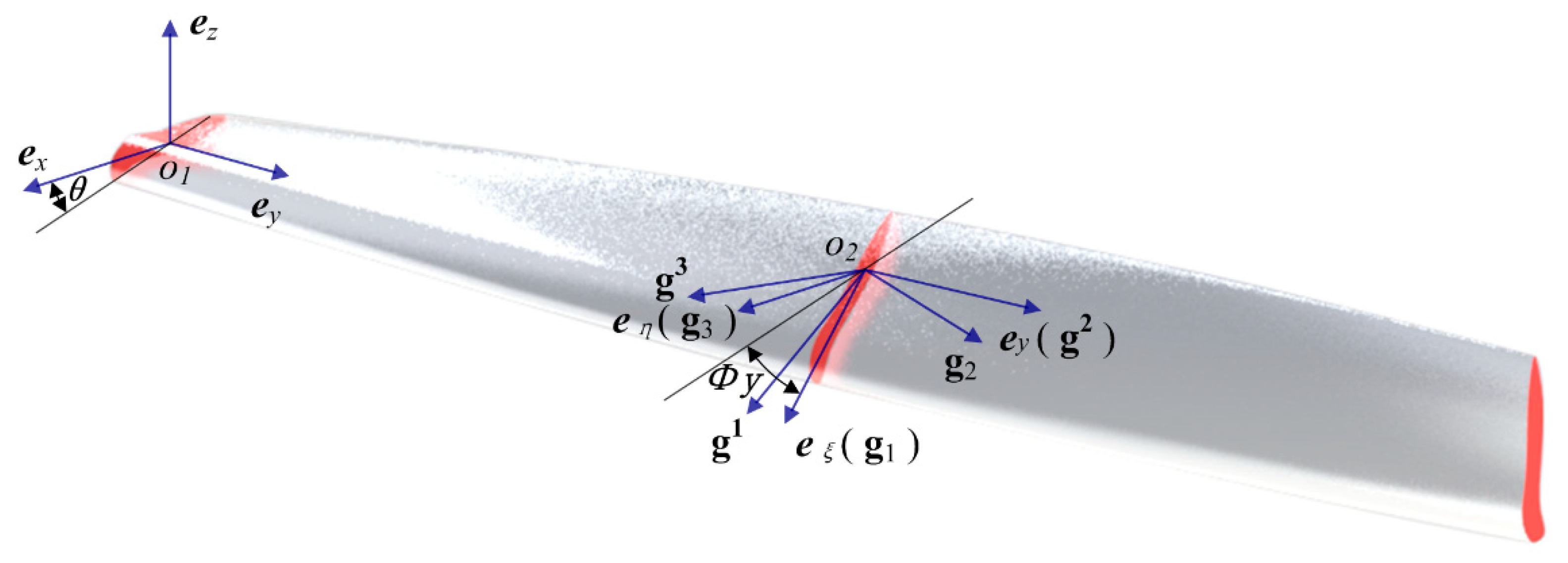
2. Kinematic Description of Pre-Twisted Structures

Figure 1 shows the geometrical description of a pre-twisted structure defined in four different coordinate systems. They are the Cartesian orthonormal basis (e_x, e_y, e_z) located at one end of the pre-twisted structure, the twisted orthonormal basis (e_ξ, e_y, e_η) translating and rotating along the longitudinal direction to trace the structural twist, and the covariant basis (g₁, g₂, g₃) and contravariant basis (g¹, g², g³) describing the deformation gradient in the twisted basis.

The twisted base vectors are related to the Cartesian coordinate system by the transformation matrix T as follows:

$$\left[\begin{array}{c}{\mathbf{e}}_{\xi }\\ {\mathbf{e}}_y\\ {\mathbf{e}}_{\eta }\end{array}\right]=\mathbf{T}\left[\begin{array}{c}{\mathbf{e}}_x\\ {\mathbf{e}}_y\\ {\mathbf{e}}_z\end{array}\right]$$

(1)

where the transformation matrix is expressed as

$$\mathbf{T}=\left[\begin{array}{ccc}\cos \left(\varphi y+\theta \right)& 0& \sin \left(\varphi y+\theta \right)\\ 0& 1& 0\\ -\sin \left(\varphi y+\theta \right)& 0& \cos \left(\varphi y+\theta \right)\end{array}\right]$$

(2)

with ϕ being the twist angle per unit length and θ as the phase angle in the y = 0 plane. For the sake of simplification, the notations c = cos(ϕy + θ) and s = sin(ϕy + θ) are introduced in the following analysis.

The position vector of any point of the structure in the twisted basis is defined as

$$\mathbf{X}(x,y,z)=\xi {\mathbf{e}}_{\xi }\left(y\right)+y{\mathbf{e}}_y+\eta {\mathbf{e}}_{\eta }\left(y\right)$$

(3)

To derive the differential operators in the twisted basis, the local covariant basis is introduced as follows:

$$\left({\mathbf{g}}_1,{\mathbf{g}}_2,{\mathbf{g}}_3\right)=\left(\partial \mathbf{X}/\partial \xi ,\partial \mathbf{X}/\partial y,\partial \mathbf{X}/\partial \eta \right)$$

(4)

From Equations (5)–(7), the relationship between the covariant basis and the twisted basis can be written as

$$\begin{array}{ccc}{\mathbf{g}}_1={\mathbf{e}}_{\xi }\left(y\right),& {\mathbf{g}}_2=-\varphi \eta {\mathbf{e}}_{\xi }\left(y\right)+{\mathbf{e}}_y+\varphi \xi {\mathbf{e}}_{\eta }\left(y\right),& {\mathbf{g}}_3=\end{array}{\mathbf{e}}_{\eta }\left(y\right)$$

(5)

and in matrix form as

$$\left\{\begin{array}{c}{\mathbf{g}}_1\\ {\mathbf{g}}_2\\ {\mathbf{g}}_3\end{array}\right\}={\left[J\right]}^{\mathrm{T}}\left\{\begin{array}{c}{\mathbf{e}}_{\xi }\\ {\mathbf{e}}_y\\ {\mathbf{e}}_{\eta }\end{array}\right\},{\left[J\right]}^{\mathrm{T}}=\left[\begin{array}{ccc}1& 0& 0\\ -\varphi \eta & 1& \varphi \xi \\ 0& 0& 1\end{array}\right]$$

(6)

The underlined covariant basis (g₁, g₂, g₃) is a local basis and varies with the material point considered. This is an obvious consequence of the curvedness of the coordinate system. This is the result of Equation (4), where the vectors of the covariant basis at a point are tangent to the three coordinate curves passing through it.

It is worth noting that in the covariant basis, the components of the vectors and the tensors are defined locally. For instance, the covariant metric tensor, defined by $g_{mn}={\mathbf{g}}_m\cdot {\mathbf{g}}_n$, is given by

$$\left(g_{mn}\right)=\left[\begin{array}{ccc}1& -\varphi \eta & 0\\ -\varphi \eta & {\varphi }^2\left({\eta }^2+{\xi }^2\right)+1& \varphi \xi \\ 0& \varphi \xi & 1\end{array}\right]$$

(7)

By introducing $\begin{array}{cc}{\mathbf{g}}_m\cdot {\mathbf{g}}^n={\delta }_m^n,& \forall m,n=1,2,3.\end{array}$, the contravariant basis (g¹, g², g³) is defined. The contravariant metric tensor components relate the covariant counterparts by the following expression:

$$\left(g_{ik}\right)\left(g^{kj}\right)=\mathbf{I}$$

(8)

Using Equations (7) and (8), the contravariant components of the metric tensor is derived as follows:

$$\left(g^{mn}\right)=\left[\begin{array}{ccc}{\varphi }^2{\eta }^2+1& \varphi \eta & -{\varphi }^2\xi \eta \\ \varphi \eta & 1& -\varphi \xi \\ -{\varphi }^2\xi \eta & -\varphi \xi & {\varphi }^2{\xi }^2+1\end{array}\right]$$

(9)

Then, we can define the local contravariant basis by the following:

$${\mathbf{g}}^m=\left({\mathbf{g}}^m·{\mathbf{g}}^n\right){\mathbf{g}}_n=g^{mn}{\mathbf{g}}_n$$

(10)

The components of the base vectors are specifically written as

$$\begin{array}{ccc}{\mathbf{g}}^1={\mathbf{e}}_{\xi }\left(y\right)+\varphi \eta {\mathbf{e}}_y,& {\mathbf{g}}^2={\mathbf{e}}_y,& {\mathbf{g}}^3=-\varphi \xi {\mathbf{e}}_y+{\mathbf{e}}_{\eta }\left(y\right)\end{array}$$

(11)

and in the matrix form as

$$\left\{\begin{array}{c}{\mathbf{g}}^1\\ {\mathbf{g}}^2\\ {\mathbf{g}}^3\end{array}\right\}=\left[K\right]\left\{\begin{array}{c}{\mathbf{e}}_{\xi }\\ {\mathbf{e}}_y\\ {\mathbf{e}}_{\eta }\end{array}\right\},\left[K\right]={\left[J\right]}^{-1}=\left[\begin{array}{ccc}1& \varphi \eta & 0\\ 0& 1& 0\\ 0& -\varphi \xi & 1\end{array}\right]$$

(12)

The Christoffel symbols of the second kind ${\mathsf{\Gamma }}_{ij}^k$, i, j, k = 1, 2, 3, associated with the covariant and contravariant bases by ${\mathsf{\Gamma }}_{ij}^k={\mathbf{g}}_{i,j}·{\mathbf{g}}^k$, are given by

$${\mathsf{\Gamma }}_{nm}^1=\left[\begin{array}{ccc}0& 0& 0\\ 0& -{\varphi }^2\xi & -\varphi \\ 0& -\varphi & 0\end{array}\right],{\mathsf{\Gamma }}_{nm}^2=\left[\begin{array}{ccc}0& 0& 0\\ 0& 0& 0\\ 0& 0& 0\end{array}\right],{\mathsf{\Gamma }}_{nm}^3=\left[\begin{array}{ccc}0& \varphi & 0\\ \varphi & -{\varphi }^2\eta & 0\\ 0& 0& 0\end{array}\right]$$

(13)

3. Nonlinear Green Lagrange Strain

The deformation components of an arbitrary point in the twisted basis can be described as

$$\left[\begin{array}{c}{u}_{\xi }\\ u_y\\ u_{\eta }\end{array}\right]=\left[\begin{array}{ccc}c& 0& s\\ 0& 1& 0\\ -s& 0& c\end{array}\right]\left[\begin{array}{c}{u}_x\\ u_y\\ u_z\end{array}\right]$$

(14)

For the displacement vector $\left\{u_{\xi },u_y,u_{\eta }\right\}$ of a specific point, the covariant and contravariant components are specified by the following expressions:

$$\begin{array}{l}{u}_i=\mathbf{u}\cdot {\mathbf{g}}_i,u^i=\mathbf{u}\cdot {\mathbf{g}}^i\\ \begin{array}{cc}\left[\begin{array}{c}{u}_1\\ u_2\\ u_3\end{array}\right]=\left[\begin{array}{c}{u}_{\xi }\\ -\varphi \eta u_{\xi }+u_y+\varphi \xi u_{\eta }\\ u_{\eta }\end{array}\right],& \left[\begin{array}{c}{u}^1\\ u^2\\ u^3\end{array}\right]=\left[\begin{array}{c}{u}_{\xi }+\varphi \eta u_y\\ u_y\\ -\varphi \xi u_y+u_{\eta }\end{array}\right]\end{array}\end{array}$$

(15)

The 3D Green–Lagrange strain tensor is given by half the increment in the 3D metric tensor. When written in the covariant basis of the curvilinear coordinate system, the strain–displacement relationship is given by

$$\begin{array}{cc}\mathsf{\epsilon }={\epsilon }_{ij}{\mathbf{g}}^i\otimes {\mathbf{g}}^j,& {\epsilon }_{ij}=\frac{1}{2}\left(u_{i|j}+u_{j|i}+u_{k|i}{u}^k{}_{|j}\right)\end{array}$$

(16)

where

$$\begin{array}{l}{u}_{i|j}=u_{i,j}-{\mathsf{\Gamma }}_{ij}^k{u}_k\\ u^i{}_{|j}=u^i{}_{,j}+{\mathsf{\Gamma }}_{kj}^i{u}^k\end{array}$$

(17)

Substituting Equations (13) and (15) into Equation (17), the first-order covariant derivatives of the covariant and contravariant displacement components are obtained as follows:

$${\left\{\begin{array}{c}{u}_{1|1}\\ u_{2|2}\\ u_{3|3}\\ u_{1|3}\\ u_{3|1}\\ u_{2|3}\\ u_{3|2}\\ u_{1|2}\\ u_{2|1}\end{array}\right\}}_l=\left[\begin{array}{ccc}{\partial }_{\xi }& 0& 0\\ {\varphi }^2\xi -\varphi \eta {\partial }_y& {\partial }_y& {\varphi }^2\eta +\varphi \xi {\partial }_y\\ 0& 0& {\partial }_{\eta }\\ {\partial }_{\eta }& 0& 0\\ 0& 0& {\partial }_{\xi }\\ -\varphi \eta {\partial }_{\eta }& {\partial }_{\eta }& \varphi \xi {\partial }_{\eta }\\ \varphi & 0& {\partial }_y\\ {\partial }_y& 0& -\varphi \\ -\varphi \eta {\partial }_{\xi }& {\partial }_{\xi }& \varphi \xi {\partial }_{\xi }\end{array}\right]\left\{\begin{array}{c}{u}_{\xi }\\ u_y\\ u_{\eta }\end{array}\right\},{\left\{\begin{array}{c}{u}^1{}_{|1}\\ u^2{}_{|2}\\ u^3{}_{|3}\\ u^1{}_{|3}\\ u^3{}_{|1}\\ u^2{}_{|3}\\ u^3{}_{|2}\\ u^1{}_{|2}\\ u^2{}_{|1}\end{array}\right\}}_l=\left[\begin{array}{ccc}{\partial }_{\xi }& \varphi \eta {\partial }_{\xi }& 0\\ 0& {\partial }_y& 0\\ 0& -\varphi \xi {\partial }_{\eta }& {\partial }_{\eta }\\ {\partial }_{\eta }& \varphi \eta {\partial }_{\eta }& 0\\ 0& -\varphi \xi {\partial }_{\xi }& {\partial }_{\xi }\\ 0& {\partial }_{\eta }& 0\\ \varphi & -\varphi \xi {\partial }_y& {\partial }_y\\ {\partial }_y& \varphi \eta {\partial }_y& -\varphi \\ 0& {\partial }_{\xi }& 0\end{array}\right]\left\{\begin{array}{c}{u}_{\xi }\\ u_y\\ u_{\eta }\end{array}\right\}$$

(18)

From Equations (16) and (18), the Green–Lagrange strain vector can be written in the contravariant basis as follows:

$${\left\{\begin{array}{c}{\epsilon }_{11}\\ {\epsilon }_{22}\\ {\epsilon }_{33}\\ 2{\epsilon }_{13}\\ 2{\epsilon }_{23}\\ 2{\epsilon }_{12}\end{array}\right\}}_l={\mathbf{b}}_{\mathrm{cov},l}\left\{\begin{array}{c}{u}_{\xi }\\ u_y\\ u_{\eta }\end{array}\right\}+{\mathbf{b}}_{\mathrm{cov},nl}\left\{\begin{array}{c}{u}_{\xi }^2\\ u_y^2\\ u_{\eta }^2\\ u_{\xi }{u}_{\eta }\\ u_{\eta }{u}_{\xi }\end{array}\right\}$$

(19)

where the expressions of b_cov,l and b_cov,nl are given in Equations (A1) and (A2), respectively.

To derive the components of the strain vectors in the twisted basis, the relationship between the deformation gradients in the twisted basis and the covariant basis is established as follows:

$$u_{\alpha ,\beta }=u_{i,j}{\left(K\right)}_{\alpha i}^{\mathrm{T}}{\left(K\right)}_{\beta j}^{\mathrm{T}}$$

(20)

where Greek subscripts α and β denote components ξ, y, and η in the twisted basis. Accordingly,

$${{\epsilon }}_{\alpha \beta }={{\epsilon }}_{ij}{\left(K\right)}_{\alpha i}^{\mathrm{T}}{\left(K\right)}_{\beta j}^{\mathrm{T}}$$

(21)

Therefore, the Green–Lagrange strain tensor can be expressed in the twisted basis as

$$\left\{\begin{array}{c}{{\epsilon }}_{\xi \xi }\\ {{\epsilon }}_{yy}\\ {{\epsilon }}_{\eta \eta }\\ 2{{\epsilon }}_{\xi \eta }\\ 2{{\epsilon }}_{y\eta }\\ 2{{\epsilon }}_{\xi y}\end{array}\right\}={\mathbf{b}}_l\left\{\begin{array}{c}{u}_{\xi }\\ u_y\\ u_{\eta }\end{array}\right\}+{\mathbf{b}}_{nl}\left\{\begin{array}{c}{u}_{\xi }^2\\ u_y^2\\ u_{\eta }^2\\ u_{\xi }{u}_{\eta }\\ u_{\eta }{u}_{\xi }\end{array}\right\}$$

(22)

where the expressions of b_l and b_nl are given in Equations (A3) and (A4), respectively.

Here, the coefficients of the differential operators used in the twisted basis (i.e., ∂ξ, ∂η, Λ) are independent of the axial coordinate. For initially twisted helical structures, the translational invariance of the differential operator coefficients is essential to assume that the beam mechanical properties do not vary along the axial direction in the twisted basis [28].

4. Constitutive Law

A constitutive law of linearly elastic material establishes a linear relationship between the second Piola–Kirchhoff stress tensor σ and the Green–Lagrange strain tensor ε by

$$\begin{array}{cc}\mathsf{\sigma }={\sigma }^{ij}{\mathbf{g}}_i\otimes {\mathbf{g}}_j,& {\sigma }^{ij}=C^{ijkl}{\epsilon }_{kl}\end{array}$$

(23)

Since these tensors are second order, the elasticity tensor is given in the covariant basis by the following fourth-order tensor:

$$\begin{array}{l}\begin{array}{cc}\mathbf{C}=C^{ijkl}{\mathbf{g}}_i\otimes {\mathbf{g}}_j\otimes {\mathbf{g}}_k\otimes {\mathbf{g}}_l,& C^{ijkl}=\lambda g^{ij}{g}^{kl}+G\left(g^{ik}{g}^{jl}+g^{il}{g}^{jk}\right)\end{array}\\ \begin{array}{cc}\lambda =\frac{\nu E}{\left(1+\nu \right)\left(1-2\nu \right)},& G=\frac{E}{2\left(1+\nu \right)}\end{array}\end{array}$$

(24)

In the twisted basis, the elasticity tensor can be defined as

$$C=C^{\alpha \beta \omega \gamma }{\mathbf{e}}_{\alpha }\otimes {\mathbf{e}}_{\beta }\otimes {\mathbf{e}}_{\omega }\otimes {\mathbf{e}}_{\gamma }$$

(25)

where the Greek subscripts α, β, δ, and γ denote the components ξ, y, and η in the twisted basis.

By introducing the Kronecker δ, the tensor components in the twisted basis are obtained as

$$\begin{array}{l}{C}^{\alpha \beta \omega \gamma }=C^{ijkl}{J}_{\alpha i}{J}_{\beta j}{J}_{\omega k}{J}_{\gamma l}=\left[\lambda g^{ij}{g}^{kl}+G\left(g^{ik}{g}^{jl}+g^{il}{g}^{jk}\right)\right]J_{\alpha i}{J}_{\beta j}{J}_{\omega k}{J}_{\gamma l}\\ =\lambda {\delta }_{\alpha \beta }{\delta }_{\omega \gamma }+G\left({\delta }_{\alpha \omega }{\delta }_{\beta \gamma }+{\delta }_{\alpha \gamma }{\delta }_{\beta \omega }\right)\end{array}$$

(26)

Finally, the elasticity coefficients that relate the stress vector to the strain vector in the twisted basis can be given by

$$C=\left[\begin{array}{cccccc}\lambda +2G& \lambda & \lambda & 0& 0& 0\\ \lambda & \lambda +2G& \lambda & 0& 0& 0\\ \lambda & \lambda & \lambda +2G& 0& 0& 0\\ 0& 0& 0& G& 0& 0\\ 0& 0& 0& 0& G& 0\\ 0& 0& 0& 0& 0& G\end{array}\right]$$

(27)

The above expression coincides with the one obtained in the Cartesian basis, as the twisted basis is orthonormal.

5. Carrera Unified Formulation

To include geometrical nonlinearity of thin structures, the displacement field is enriched with the higher order terms in the framework of the Carrera unified formulation (CUF). Herein, the displacement vector u at any point is approximated by the following expression:

$$\begin{array}{cc}\mathbf{u}\left(\xi ,y,\eta ,t\right)=F_s\left(\xi ,\eta \right)N_j\left(y\right){\mathbf{q}}_{sj}\left(t\right),& s=1,2,\cdots ,M_u\end{array}$$

(28)

where q_sj is the generalized displacement vector, N_j represents the shape functions along the axial direction, and F_s denotes the expansion functions of the beam cross section, with M_u as the order of F_s. Here, we use Einstein’s summation convention—i.e., summation signs are not written for all indices that repeat once as a subscript and once as a superscript in an expression. Additionally, subscripts and superscripts s and j are called dummy indices, since they can be replaced by any other letters—i.e., τ and i.

Several different types of polynomials could be used to construct the expansion functions describing the cross-sectional geometry, including Taylor expansions (TE), Lagrange expansions (LE), and Hierarchical Legendre expansions (HLE). The TE expands the polynomial globally over the cross section from the beam axis, while the LE beam theories discretize the cross section physical surface into a number of local expansion sub-domains, whose polynomial degree depends on the type of Lagrange expansion employed. Three-node linear L3, four-node bilinear L4, nine-node quadratic L9, and sixteen-node cubic L16 polynomials have been developed in the framework of CUF. HLE models combine the main features of the previous beam theories, including the hierarchy of the high-order terms of TE and the geometric discretization of the beam section surface of LE. For the sake of brevity, their expressions are not included here, but they can be found in the literature [29].

In the framework of CUF, the strain vector in the twisted basis is calculated as follows:

$$\mathsf{\epsilon }=\left({\mathbf{B}}_l^{sj}+{\mathbf{B}}_{nl\_1}^{sj}+{\mathbf{B}}_{nl\_2}^{sj}\right){\mathbf{q}}_{sj}$$

(29)

where the expressions of $B_l^{sj}$, $B_{nl\_1}^{sj}$, and $B_{nl\_2}^{sj}$ are given in Equations (A5)–(A7), respectively.

The stress vector and the virtual variation of the strain vector are derived in terms of the generalized displacement vector as

$$\begin{array}{l}\mathsf{\sigma }=\mathbf{C}\left(B_l^{sj}+B_{nl}^{sj}\right)q_{sj}\\ \delta \mathsf{\epsilon }=\delta \left(\left(B_l^{\tau i}+B_{nl}^{\tau i}\right){\mathbf{q}}_{\tau i}\right)=\left(B_l^{\tau i}+2B_{nl}^{\tau i}\right)\delta q_{\tau i}\end{array}$$

(30)

6. Equations of Motion

Substituting the stress and strain vectors, the variation of the elastic potential energy δU is given by

$$\delta U={\displaystyle {\int }_V\delta {\mathsf{\epsilon }}^{\mathrm{T}}\mathsf{\sigma }dV}=\delta {\mathbf{q}}_{\tau i}^{\mathrm{T}}{\displaystyle {\int }_V{\left(B_l^{\tau i}+2B_{nl}^{\tau i}\right)}^{\mathrm{T}}C\left(B_l^{sj}+B_{nl}^{sj}\right)dV}{\mathbf{q}}_{sj}$$

(31)

According to the definition, the secant stiffness matrix $K_s^{ij\tau s}$ relates to the strain energy by

$$\begin{array}{cc}\delta U=\delta {\mathbf{q}}_{\tau i}^{\mathrm{T}}{\mathbf{K}}_s^{ij\tau s}{\mathbf{q}}_{sj},& {\mathbf{K}}_s^{ij\tau s}={\mathbf{K}}_l^{ij\tau s}+{\mathbf{K}}_{lnl}^{ij\tau s}+{\mathbf{K}}_{nll}^{ij\tau s}+{\mathbf{K}}_{nlnl}^{ij\tau s}\end{array}$$

(32)

where $K_l^{ij\tau s}$ represents the linear component, $K_{lnl}^{ij\tau s}$ and $K_{nll}^{ij\tau s}$ are the first-order nonlinear contributions, and $K_{n\ln l}^{ij\tau s}$ contains the second-order nonlinearities. They are expressed as

$$\begin{array}{cc}{\mathbf{K}}_l^{ij\tau s}={\displaystyle {\int }_V{\left(B_l^{\tau i}\right)}^{\mathrm{T}}C{B}_l^{sj}dV},& {\mathbf{K}}_{lnl}^{ij\tau s}={\displaystyle {\int }_V{\left(B_l^{\tau i}\right)}^{\mathrm{T}}C{B}_{nl}^{sj}dV}\\ {\mathbf{K}}_{nll}^{ij\tau s}=2{\displaystyle {\int }_V{\left(B_{nl}^{\tau i}\right)}^{\mathrm{T}}C{B}_l^{sj}dV},& {\mathbf{K}}_{nlnl}^{ij\tau s}=2{\displaystyle {\int }_V{\left(B_{nl}^{\tau i}\right)}^{\mathrm{T}}C{B}_{nl}^{sj}dV}\end{array}$$

(33)

Since the secant stiffness matrix is generally not symmetrical, the numerical results are merely with low orders of convergence. A symmetrical tangent stiffness matrix can be derived by linearizing the virtual variation of the strain energy as follows:

$$\delta \left(\delta U\right)=\delta {\displaystyle {\int }_V\delta {\mathsf{\epsilon }}^{\mathrm{T}}\mathsf{\sigma }dV}={\displaystyle {\int }_V\delta \left(\delta {\mathsf{\epsilon }}^{\mathrm{T}}\right)\mathsf{\sigma }+\delta {\mathsf{\epsilon }}^{\mathrm{T}}\delta \mathsf{\sigma }dV}=\delta {\mathbf{q}}_{\tau i}^{\mathrm{T}}{K}_{\mathrm{T}}^{ij\tau s}{\mathbf{q}}_{sj}$$

(34)

From Equation (29), the linearization of the virtual variation of the strain is calculated as

$$\delta \left(\delta {\mathsf{\epsilon }}^{\mathrm{T}}\right)={\left[\begin{array}{l}\delta q_{\xi \tau i}\delta q_{\xi sj}\hfill \\ \delta q_{y\tau i}\delta q_{ysj}\hfill \\ \delta q_{\eta \tau i}\delta q_{\eta sj}\hfill \\ \delta q_{\xi \tau i}\delta q_{\eta sj}\hfill \\ \delta q_{\eta \tau i}\delta q_{\xi sj}\hfill \end{array}\right]}^{\mathrm{T}}{\left(B_{nl}^{*}\right)}^{\mathrm{T}}={\left[\begin{array}{c}\delta q_{\xi \tau i}\delta q_{\xi sj}\\ \delta q_{y\tau i}\delta q_{ysj}\\ \delta q_{\eta \tau i}\delta q_{\eta sj}\end{array}\right]}^{\mathrm{T}}{\left(B_{nl\_1}^{*}\right)}^{\mathrm{T}}+{\left[\begin{array}{c}\delta q_{\xi \tau i}\delta q_{\eta sj}\\ \delta q_{\eta \tau i}\delta q_{\xi sj}\end{array}\right]}^{\mathrm{T}}{\left(B_{nl\_2}^{*}\right)}^{\mathrm{T}}$$

(35)

where $B_{nl\_1}^{*}$ and $B_{nl\_2}^{*}$ are given in Equations (A9) and (A10), respectively.

Then, the first contribution of the virtual variation of the strain energy δ(δU) is derived as

$${\displaystyle {\int }_V\delta \left(\delta {\mathsf{\epsilon }}^{\mathrm{T}}\right)\mathsf{\sigma }dV}={\displaystyle {\int }_V\left\{{\left[\begin{array}{c}\delta q_{\xi \tau i}\delta q_{\xi sj}\\ \delta q_{y\tau i}\delta q_{ysj}\\ \delta q_{\eta \tau i}\delta q_{\eta sj}\end{array}\right]}^{\mathrm{T}}{\left(B_{nl\_1}^{*}\right)}^{\mathrm{T}}+{\left[\begin{array}{c}\delta q_{\xi \tau i}\delta q_{\eta sj}\\ \delta q_{\eta \tau i}\delta q_{\xi sj}\end{array}\right]}^{\mathrm{T}}{\left(B_{nl\_2}^{*}\right)}^{\mathrm{T}}\right\}\mathsf{\sigma }dV}=\delta {\mathbf{q}}_{\tau i}^{\mathrm{T}}{K}_{\sigma }^{ij\tau s}\delta {\mathbf{q}}_{sj}$$

(36)

where the expression of $K_{\sigma }^{ij\tau s}$ is given in Equation (A11).

The second term of the virtual variation of the strain energy δ(δU) is defined as

$${\displaystyle {\int }_V\delta {\mathsf{\epsilon }}^{\mathrm{T}}\delta \mathsf{\sigma }dV}=\delta {\mathbf{q}}_{\tau i}^{\mathrm{T}}{\displaystyle {\int }_V{\left(B_l^{\tau i}+2B_{nl}^{\tau i}\right)}^{\mathrm{T}}C\left(B_l^{sj}+2B_{nl}^{sj}\right)dV}{\mathbf{q}}_{sj}=\delta {\mathbf{q}}_{\tau i}^{\mathrm{T}}\left(K_l^{ij\tau s}+K_{\mathrm{T}1}^{ij\tau s}\right){\mathbf{q}}_{sj}$$

(37)

where

$$K_{\mathrm{T}\_1}^{ij\tau s}=2K_{lnl}^{ij\tau s}+K_{nll}^{ij\tau s}+2K_{nlnl}^{ij\tau s}$$

(38)

Combining Equations (34), (36) and (37), the tangent stiffness matrix is given by

$$K_{\mathrm{T}}^{ij\tau s}=K_l^{ij\tau s}+K_{\mathrm{T}1}^{ij\tau s}+K_{\sigma }^{ij\tau s}$$

(39)

where $K_l^{ij\tau s}$, $K_{\mathrm{T}1}^{ij\tau s}$, and $K_{\sigma }^{ij\tau s}$ are the linear stiffness matrix, the nonlinear stiffness matrix, and the geometrically stiffening stiffness matrix, respectively. Unlike Ks, all the contributions of the tangent stiffness matrix are symmetrical.

When the pre-twist contributions are not included, the secant and tangent stiffness matrices have the same expression as those given by [30]. If the pre-twist terms are included, the strong coupling of nonlinear axial and cross-sectional deformations is reflected.

As for the external work, the contributions from volume forces g, surface forces p, line forces q, and concentrated force P at point Q are considered. The variation of the external work is written as

$$\begin{array}{l}\delta L_{ext}={\displaystyle {\int }_V\delta {\mathbf{u}}^{\mathrm{T}}\mathbf{g}dV}+{\displaystyle {\int }_S\delta {\mathbf{u}}^{\mathrm{T}}pdS}+{\displaystyle {\int }_L\delta {\mathbf{u}}^{\mathrm{T}}\mathbf{q}dy}+{\delta {\mathbf{u}}^{\mathrm{T}}|}_{Q}P\\ =\delta q_{\tau i}^{\mathrm{T}}\left({\displaystyle {\int }_V{F}_{\tau }{N}_i\mathbf{g}dV}+N_i{\displaystyle {\int }_S{F}_{\tau }pdS}+F_{\tau }{\displaystyle {\int }_{L}qdy}+F_{\tau }{N}_{i}P\right)\end{array}$$

(40)

From Equation (32), the nonlinear governing equation is formulated as follows:

$$K_s^{ij\tau s}{\mathbf{q}}_{sj}=F_{\tau i}$$

(41)

where the generalized force vector F_τi is expressed as

$$F_{\tau i}={\displaystyle {\int }_V{F}_{\tau }{N}_{i}gdV}+N_i{\displaystyle {\int }_S{F}_{\tau }pdS}+F_{\tau }{\displaystyle {\int }_{L}qdy}+F_{\tau }{N}_{i}P$$

(42)

7. Arc-Length Method

Using Crisfield’s arc-length method, Equation (41) is rewritten as

$$R_{\tau i}=\lambda F_{\tau i}-K_s^{ij\tau s}{\mathbf{q}}_{sj}$$

(43)

where R_τi represents the generalized out-of-balance force vector, and λ is the scalar load parameter.

Along the response curve of the nonlinear deformation, the incremental expression of the governing equation becomes

$$\Delta \lambda F_{\tau i}-K_{\mathrm{T}}^{ij\tau s}\Delta {\mathbf{q}}_{sj}=0$$

(44)

At any incremental step of the converged solution, the iteration direction is orthogonal to the tangent of the response curve. By fixing the length of the incremental step, the constraint equation with a constant arc length is formulated as

$$\Delta {\mathbf{q}}_{sj}^{\mathrm{T}}\Delta {\mathbf{q}}_{sj}+{\left(\Delta \lambda \right)}^2={\left(\Delta S\right)}^2$$

(45)

where ∆S is the finite increment of the arc length.

The generalized displacement increment at iteration m from step p to p + 1 can be expressed as

$${\mathbf{q}}_{sj}^{p,m+1}={\mathbf{q}}_{sj}^m-{\mathbf{q}}_{sj}^p+\Delta {\mathbf{q}}_{sj}^{R,m}+\Delta {\lambda }^m\Delta {\mathbf{q}}_{sj}^{F,m}$$

(46)

where

$$\begin{array}{l}\Delta q_{sj}^{R,m}={\left(K_{\mathrm{T},m}^{ij\tau s}\right)}^{-1}{R}_{\tau i}^m\\ \Delta q_{sj}^{F,m}={\left(K_{\mathrm{T},m}^{ij\tau s}\right)}^{-1}{F}_{\tau i}\end{array}$$

(47)

Then, the quadratic constraint equation at iteration m from step p to p + 1 is given by

$$a{\left(\Delta {\lambda }^m\right)}^2+2b\left(\Delta {\lambda }^m\right)+c=0$$

(48)

with

$$\begin{array}{l}a={\left(\Delta q_{sj}^{F,m}\right)}^{\mathrm{T}}\Delta q_{sj}^{F,m}\\ b=\Delta q_{sj}^{F,m}{p}_{sj}^m\\ c={\left(p_{sj}^m\right)}^{\mathrm{T}}{p}_{sj}^m-{\left(\Delta S\right)}^2\\ p_{sj}^m=q_{sj}^m-q_{sj}^p+\Delta q_{sj}^{R,m}\end{array}$$

(49)

The appropriate generalized displacement increment solution can be evaluated by imposing the least angle between ${\mathbf{q}}_{sj}^{p,m}$ and ${\mathbf{q}}_{sj}^{p,m+1}$.

8. Results

The nonlinear deformation simulation of three kinds of pre-twisted structures are presented in this section. Figure 2, Figure 3 and Figure 4 show the simplified geometries of pre0twisted structures with rectangular, arc profile, and airfoil profile cross sections, respectively. All those structures are assumed to be uniformly pre-twisted and the dimensions are listed in

Table 1. Physical properties of pre-twisted structures.

Properties	Rectangular Cross-Sectional Structure	Arc profile Cross-Sectional Structures	Airfoil Profile Cross-Sectional Structure
Length Ɩ	152.4 mm	710 mm	500 mm
Width b	25.4 mm	305 mm	100 mm
Thickness h	1.7272 mm	3.05 mm	5 mm (maximum)
Arc angle α	-	30°, 60°, 90°	-
Pretwist angle k	45°	30°, 60°	45°

.

The rectangular cross section is characterized by the width b₁ and the height h₁, and the pre-twist center P₁ coincides with the geometrical center C₁. The physical properties of the arc profile cross sections are taken from widely investigated twisted cylindrical panels [31]. These dimensions give shell configurations with the same width b₂ and thickness h₂, and the pre-twist center P₂ is located at the center of the middle arc chord. The arc profile cross-sectional structures are distinguished from each other by the arc angle θ₂ and the pre-twist angle k₂. As for the airfoil profile section, the same NACA-8405 geometry is selected in accordance with the authors’ previous paper [2]. The 4 digits define the maximum camber, its position, and the maximum thickness, and the pre-twist center P₃ is located at the geometrical center C₃ of the airfoil section. The material of these structures is assumed to be aluminum alloy, with Young’s modulus of 70GPa and Poisson’s ratio of 0.3.

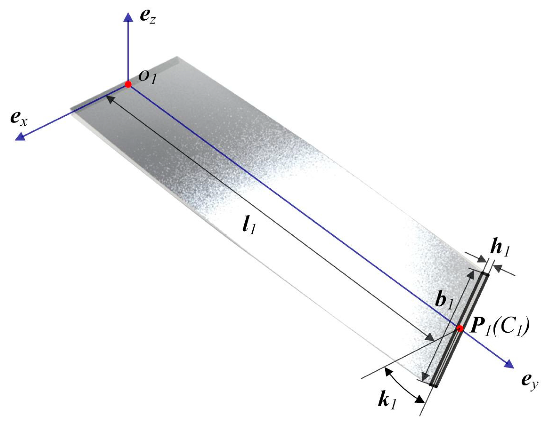
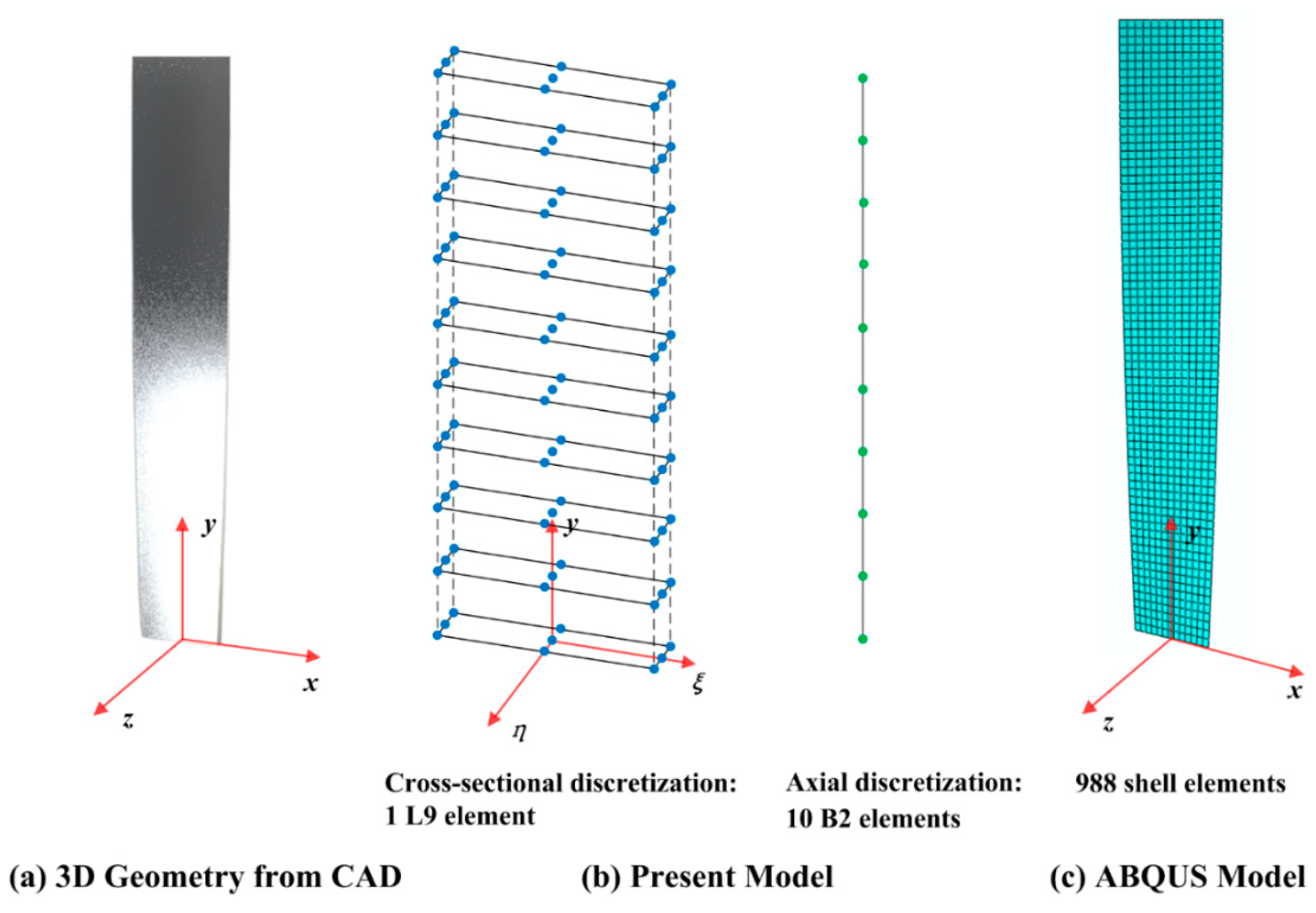
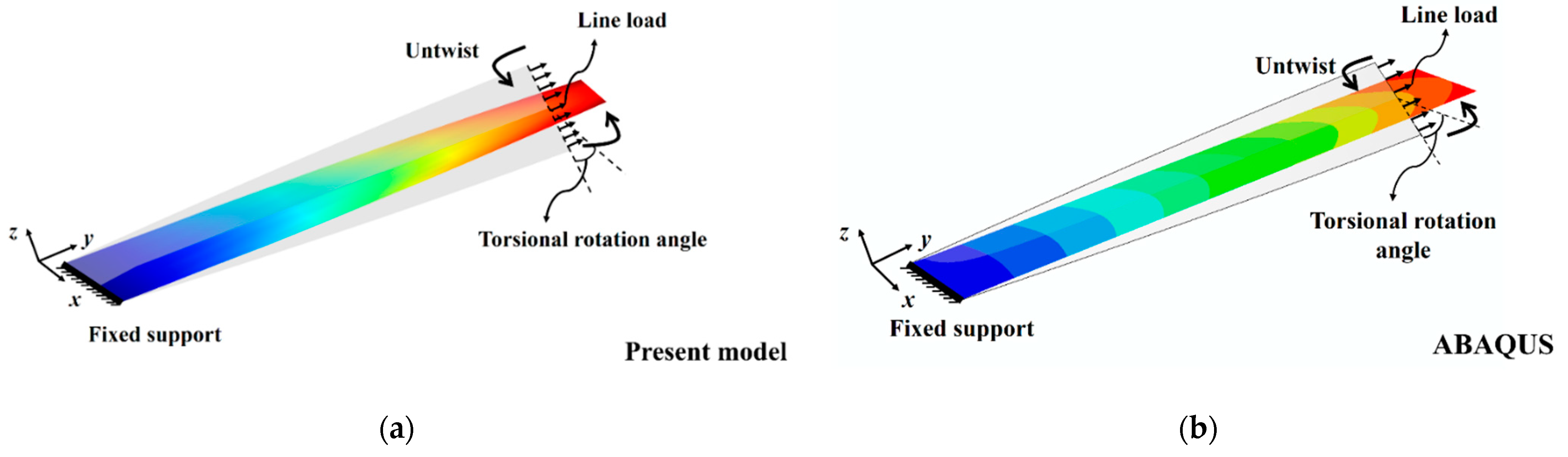
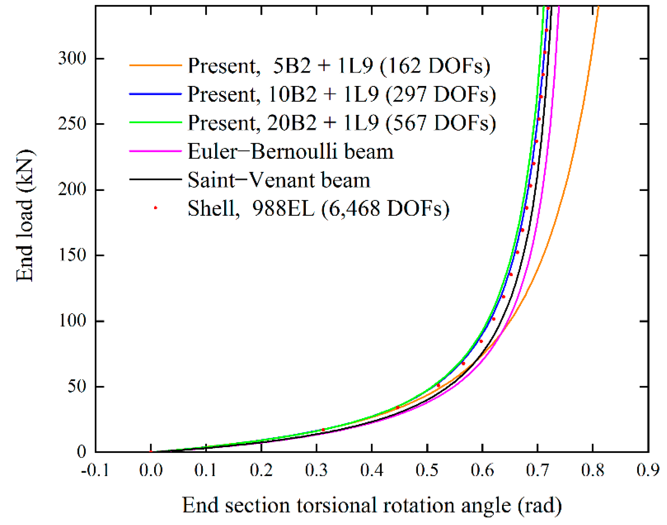
8.1. Pretwisted Cantilever with Rectangular Cross Section

A thin-walled, rectangular, cross-sectional cantilever with 45° pre-twist is first considered. A uniformly distributed longitudinal load (338 kN in total) is applied to the free-end cross section, resulting in the untwisting of the structure.

In our model, depicted in Figure 5b, one L9 Lagrange element is implemented to describe the cross-sectional displacement field. In the longitudinal direction, 5, 10, and 20 two-node (B2) beam elements are applied for discretization to study the convergence rate. The corresponding degree of freedoms (DOFs) are 162, 297, and 567. The obtained nonlinear deformation results are compared with those obtained by shell models from ABAQUS, a popular commercial software. To achieve stable convergence, the shell model consists of 988 quadrilateral elements shown in Figure 5c, with a total DOF of 6468.

Figure 6 shows the 3D structural configurations obtained from 10 B2 + 1 L9 CUF model and ABAQUS shell model, respectively. Results show that the nonlinear axial–torsional coupling of the cantilever is accurately captured. The whole structure undergoes a large untwist deformation under the applied longitudinal load. This interesting phenomenon is attributed to the coupling of torsion and extension through pre-twist. Actually, the axial stress component becomes inclined in the twisted basis and generates a net torque that twists the structure in the direction opposite to its initial torsion. The rotational center of the cross section coincides with the pre-twist center of the structure. Moreover, the free-end section keeps the rectangular profile, which reflects the mechanical property of the thin-walled structure.

Figure 7 plots the rotation of the beam free-end section obtained by the present theory, Euler–Bernoulli beam theory [32], Saint-Venant beam theory [33], and shell finite element results. For the present method, equal or more than 10 B2 elements are required to obtain results consistent with those obtained by the shell model. The maximum difference of the torsional rotational angle between the 1 L9 + 10 B2 model and ABAQUS model is 1%, indicating that the present method is more accurate than traditional beam theory. With a total end load of 338 kN, the untwisted angle is approximately 0.72rad (41.25°). Therefore, the deformed structure is nearly straight after untwisting.

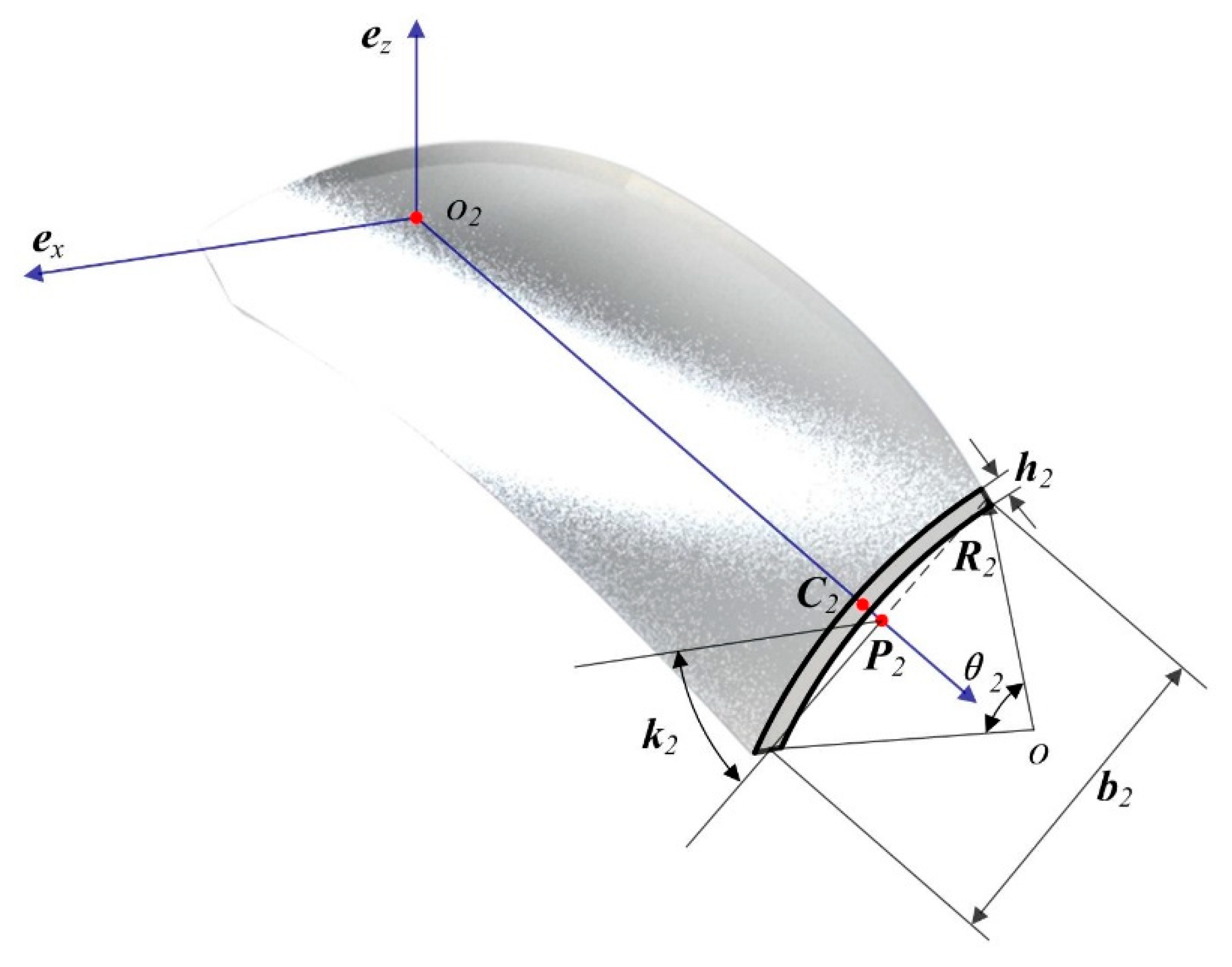
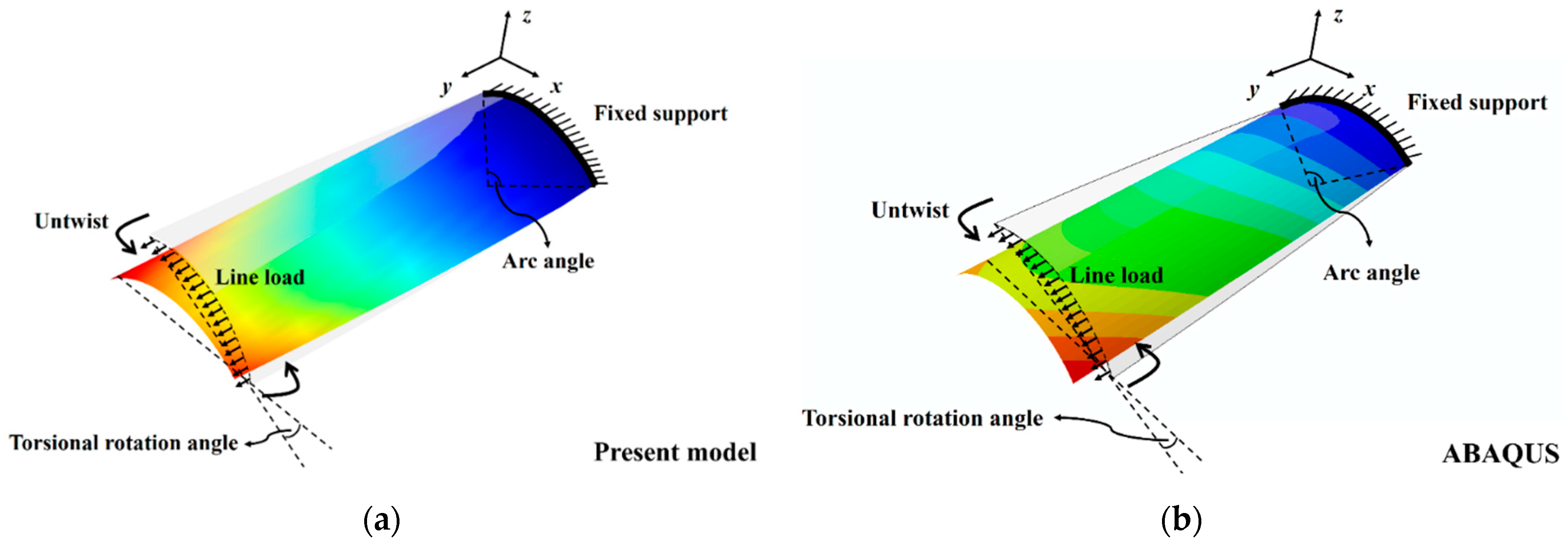
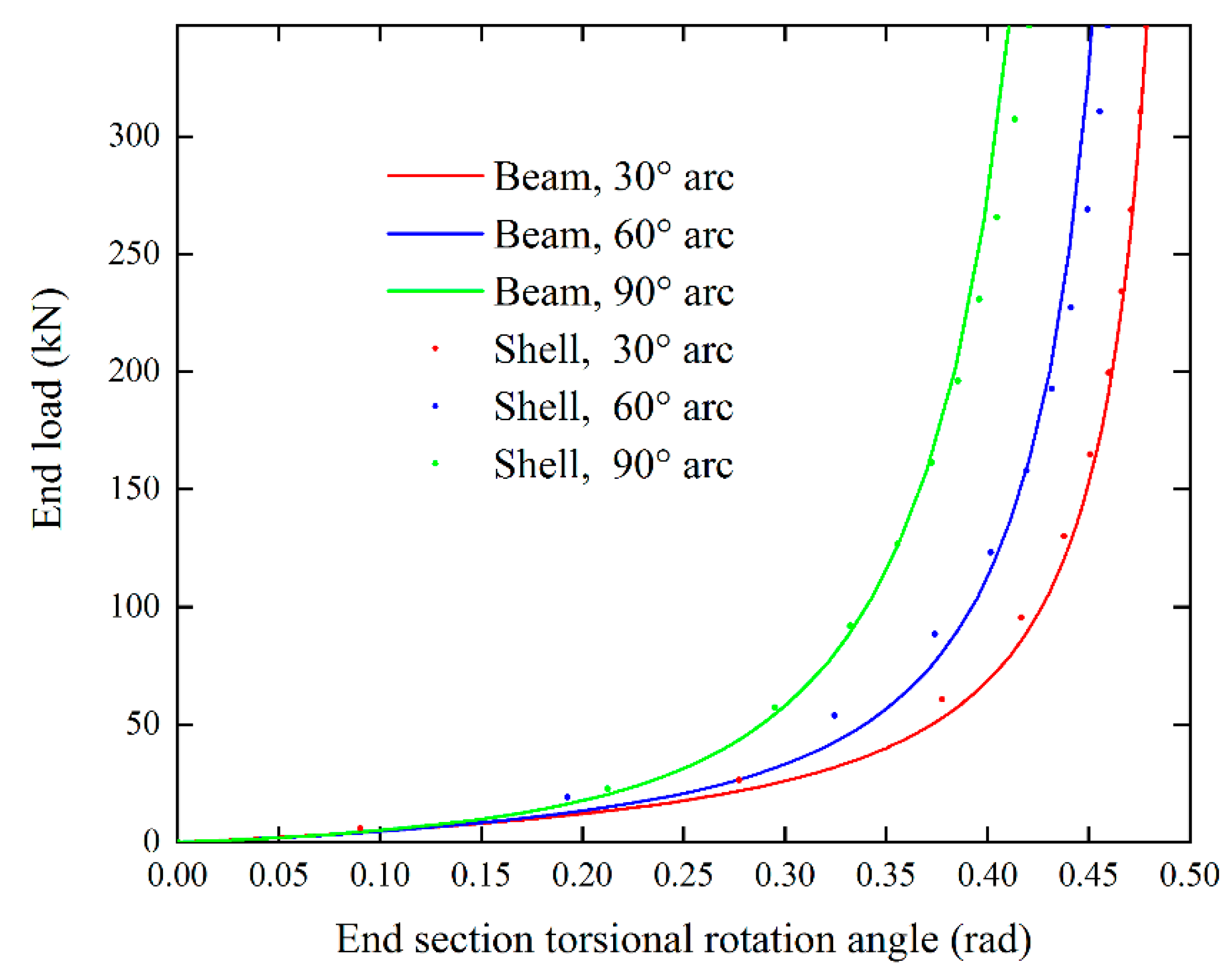
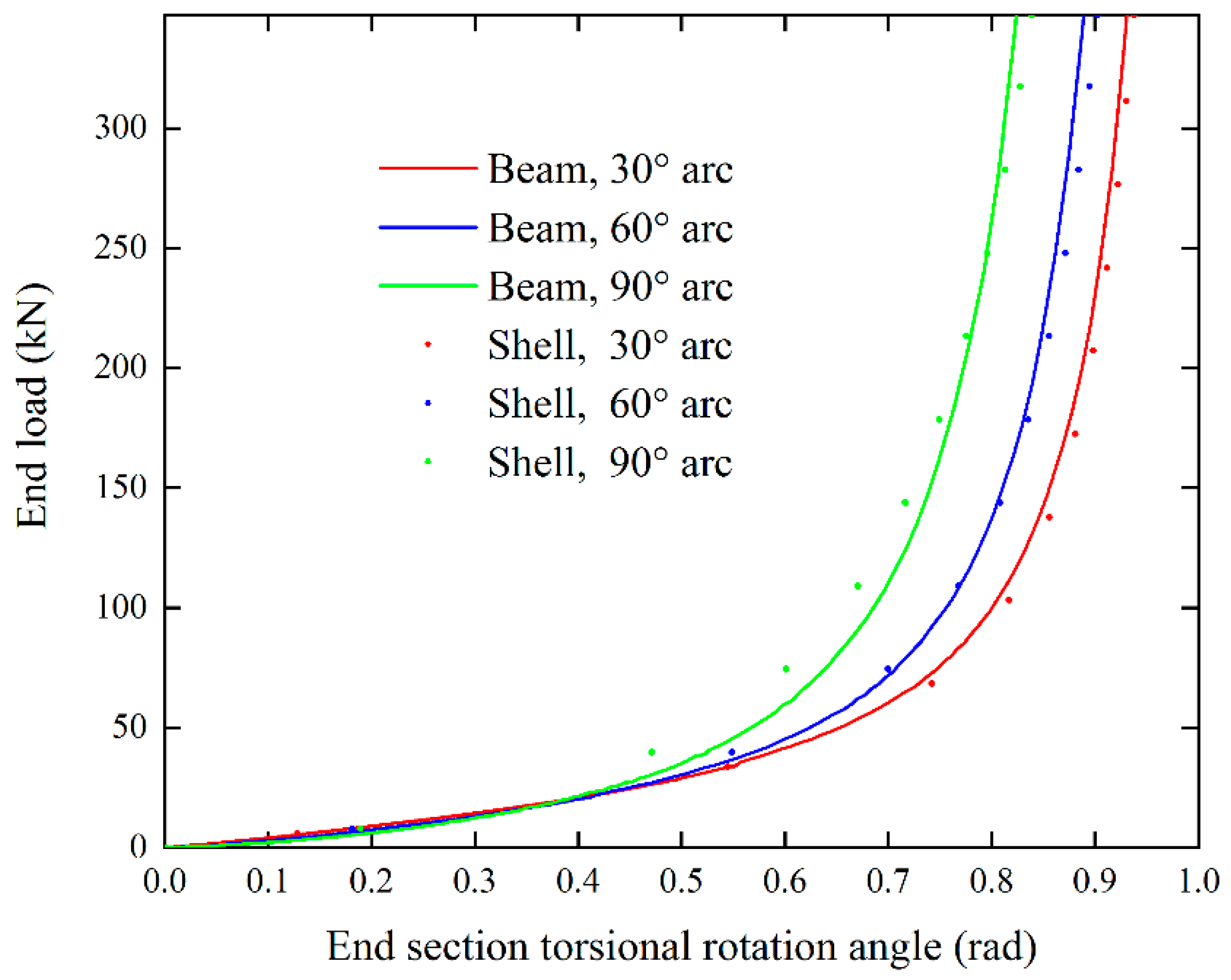
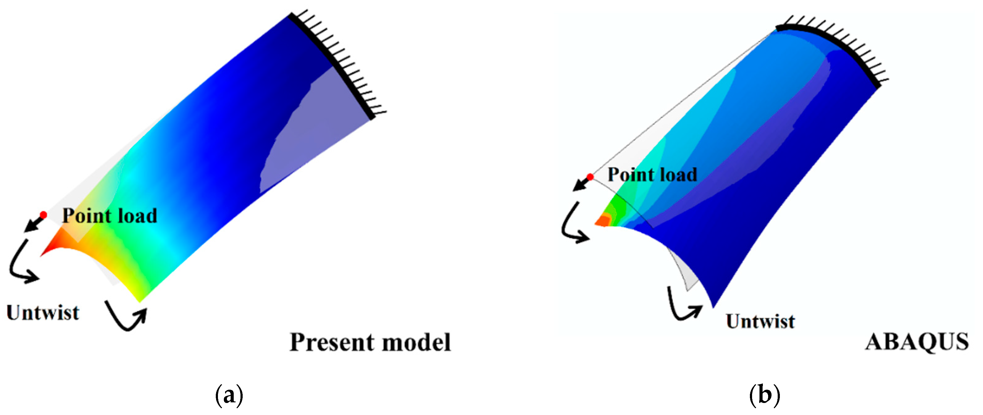
8.2. Pretwisted Cantilever with arc Profile Cross Section

Pre-twisted structures with different cross-sectional arc angles and pre-twist angles are studied. First, a uniformly distributed axial load (347 kN in total) is applied to the free-end cross section.

As shown in Figure 8b, one L9 element is implemented to construct the physical boundary and the second-order displacement field within the cross section. Since L9 set polynomials can be seen as parabolic expansions plus cubic and quartic terms, the use of these polynomials allows for an accurate description of the second-order cross-sectional field. In addition, 10 B2 elements are exploited along the longitudinal direction.

The present method formulates the governing equation using axially invariant elements with a separated structural pre-twist. Thus, we can use the same elements to discretize pre-twisted structures with any pre-twist angle, as long as their cross-sectional geometry remains the same. In other words, for pre-twisted structures with different pre-twist angles, we only need to mesh the structures once. Therefore, the complexity and cost of constructing the governing equation are greatly reduced.

The present nonlinear simulation results are compared with those obtained from commercial shell models. As shown in Figure 8c, the shell model in ABAQUS uses the same discretization of 1008 quadrilateral elements. This discretization with 6468 DOFs is found to be the proper choice for achieving stable convergence.

Figure 9 provides the 3D structural configurations of a 30° pre-twisted cantilever with a 90° arc-shaped cross section. Comparison results are given for 10 B2 + 1 L9 CUF model and ABAQUS shell model with uniform end loads. It is shown that the present model can accurately capture the nonlinear axial-torsional coupling of the cantilever, with the torsional center consistent with the pre-twist center. The deformed structure is almost straight after untwisting and the free-end section maintains the arc profile.

Then, the effect of geometric differences on the nonlinear deformation results is investigated. Figure 10 and Figure 11 show the end section torsional rotational angles of 30° and 60° pre-twisted shells with different arc angles, respectively. The rotation angles calculated by the present theory are consistent with those obtained by ABAQUS. For cantilevers with 30°, 60°, and 90° arc profile sections, the maximum differences are 3.2%, 6%, and 2.5%, respectively.

As shown in Figure 10, the torsional angle shows a maximum reduction of 23% as the arc angle increases from 30° to 90°. Correspondingly, this reflects a 30% increase in the torsional stiffness, while in Figure 11, the maximum reduction in the torsional angle is 15%, and the torsional stiffness increases by 17%. In all, a pre-twisted structure with larger cross-sectional curvature has higher stiffness and undergoes less untwisting. Therefore, structural stiffening can be achieved by increasing the structural curvature. However, this stiffening decreases when the initial twist increases.

Finally, the large deformation analysis of a pre-twisted cantilever with central and edge point loads is performed. Here, 4 L9 cross-sectional elements and 10 B2 axial elements are used to solve the problem. As shown in Figure 12, the present model can accurately capture the local deformations around the point of application of the force. In Figure 13, the present model can accurately capture coupled axial, torsional, and flexure deformations, as well as the local deformations around the point of application of the force.

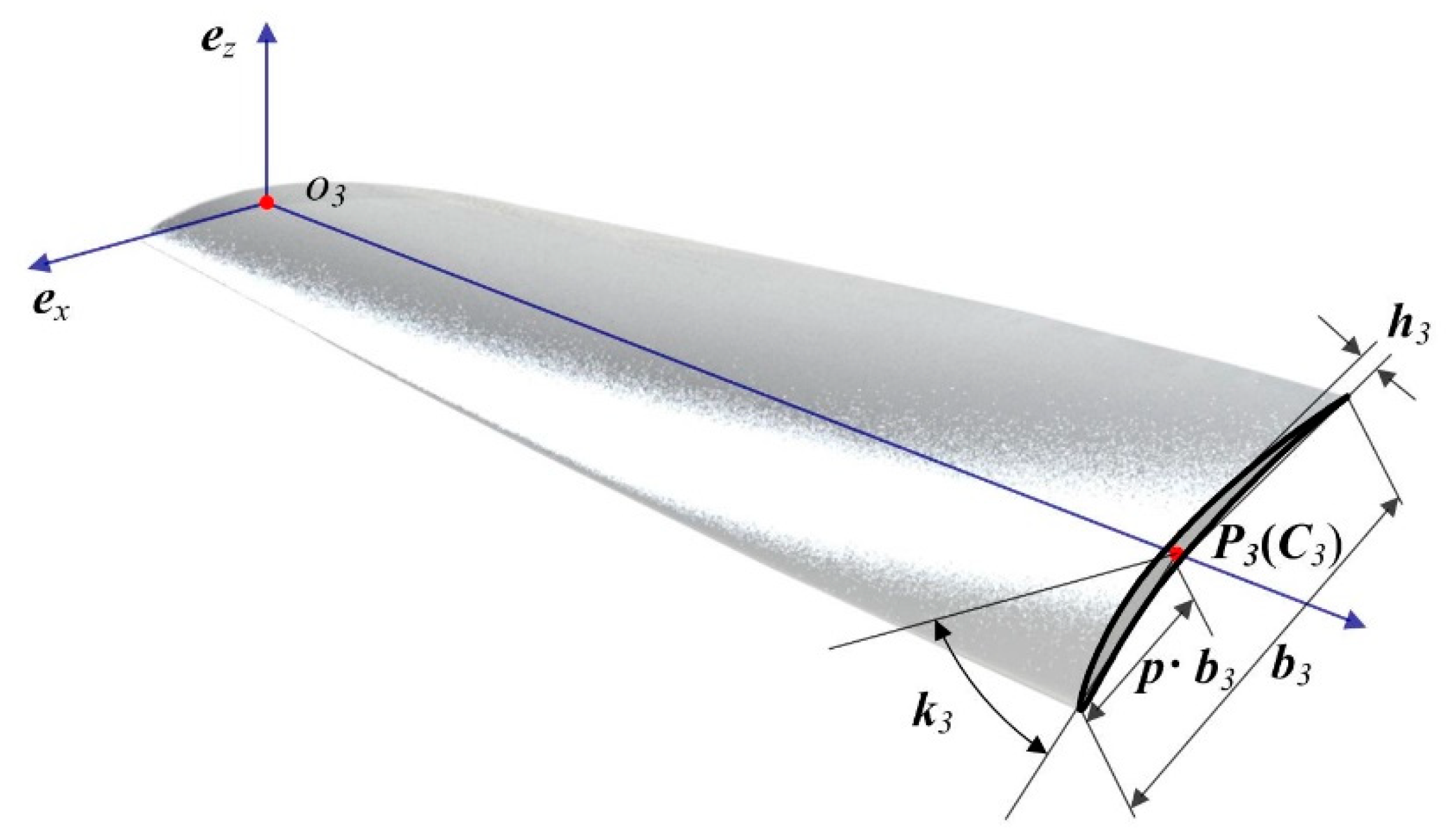
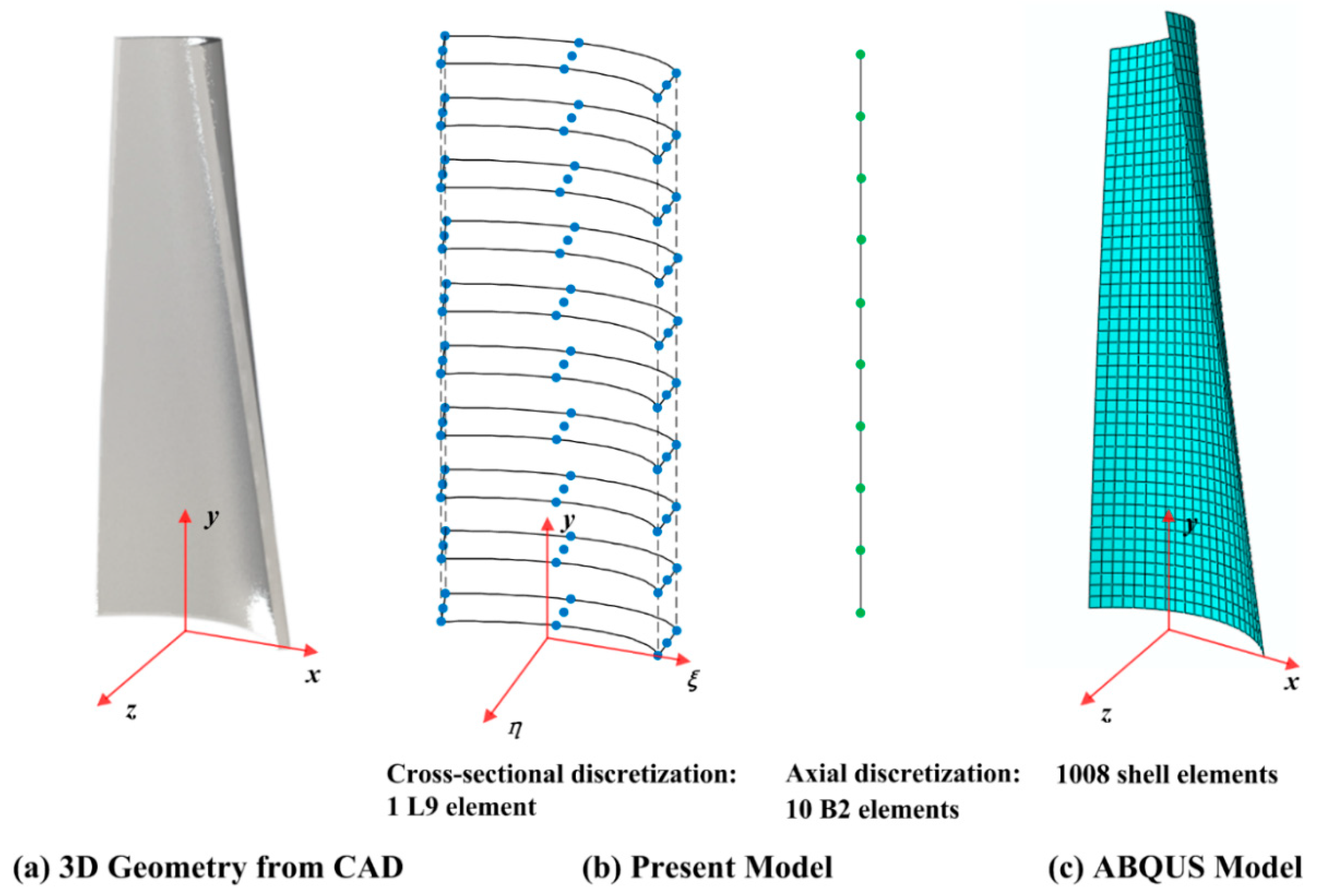
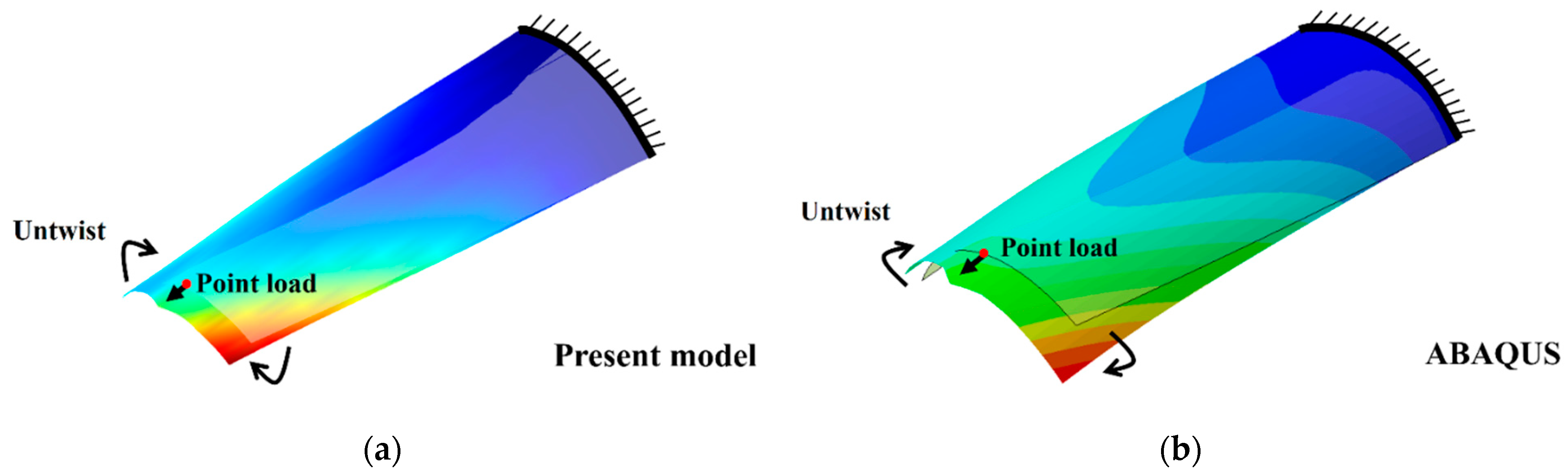
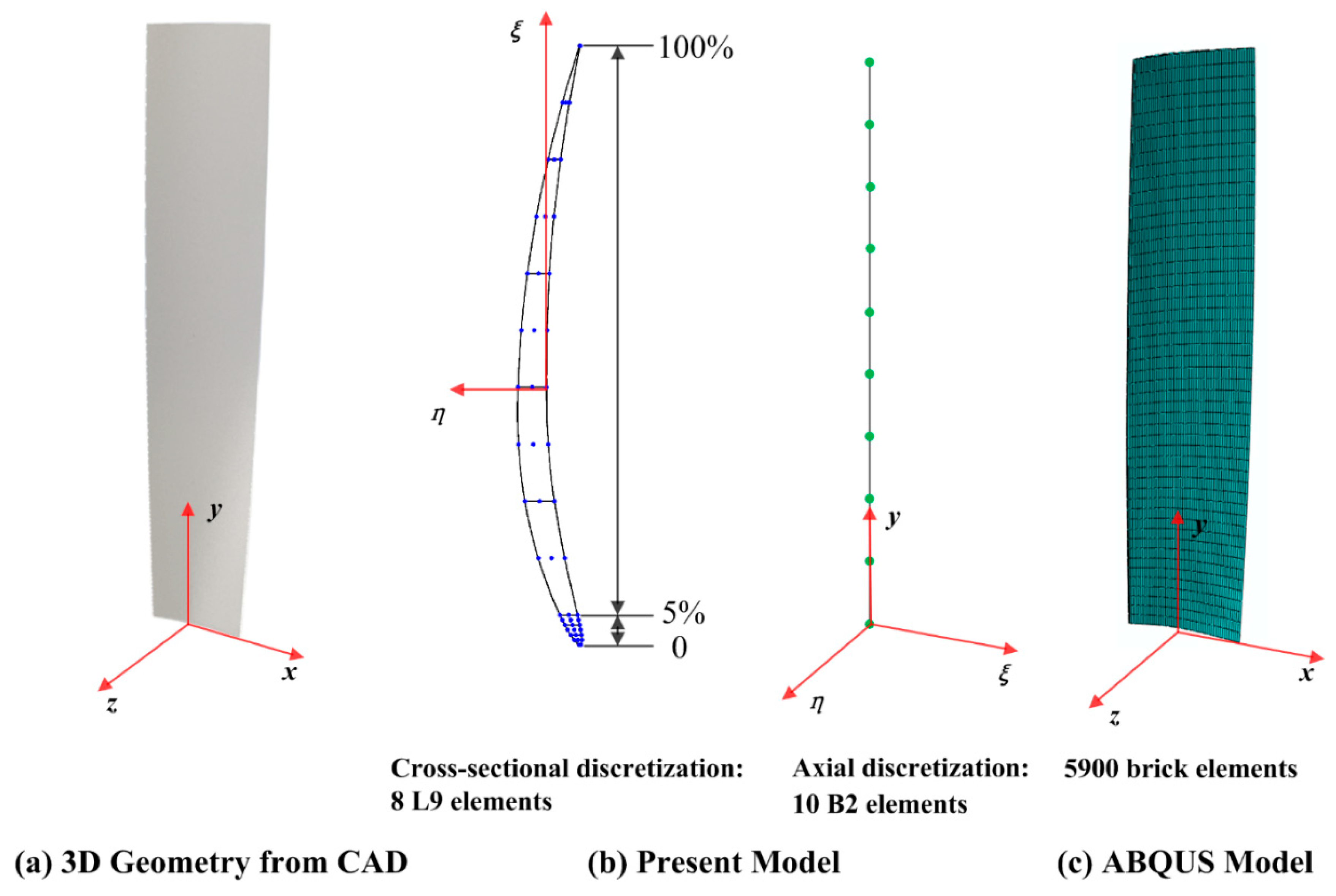
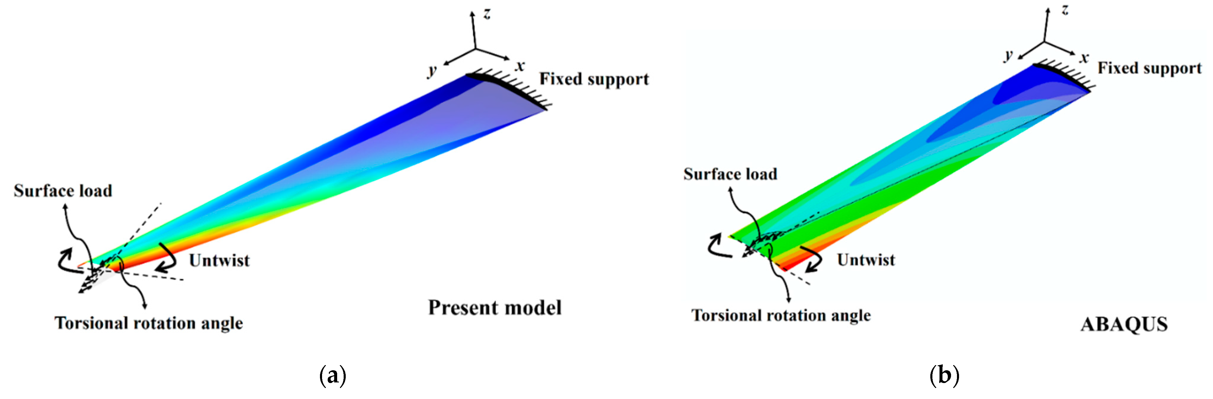
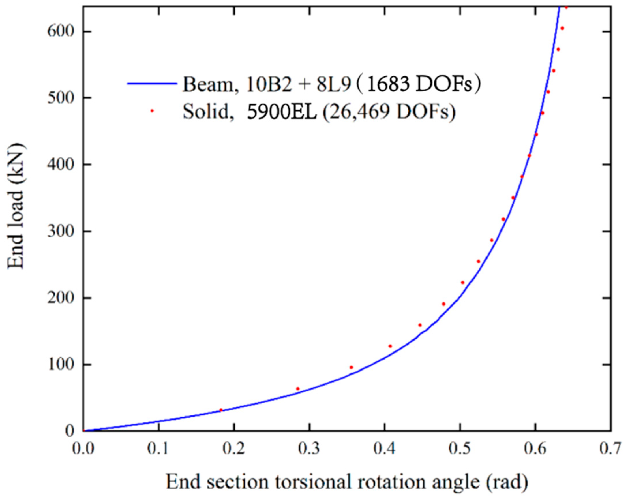
8.3. Pretwisted Cantilever with Airfoil Profile Cross Section

A pre-twisted airfoil profile cantilever with NACA 8405 dimensions is investigated. A uniformly distributed longitudinal load (636 kN in total) is applied to the free-end cross section.

Ten B2 and 8 L9 elements are found to be proper discretization choices to simulate the nonlinear deformation. Figure 14b plots the L9 element distribution in the cross section. In the 0–5% section of the camber line, the curvature of the thickness distribution changes relatively rapidly. Therefore, 3 L9 elements are implemented to construct the cross-sectional displacement field. As for the remaining 95% section, it is appropriate to select 5 L9 elements to describe the smooth camber line and thickness distribution. In the ABAQUS solid model, 5900 hexahedral elements are needed to achieve convergence. Each element contains 8 3-DOF nodes and the total number of DOFs is 26,469, as shown in Figure 14c.

Comparison results are given for the torsional rotation of the end section and the 3D deformed configuration of the whole structure. The results presented in Figure 15 and Figure 16 show good agreement. The maximum difference in the torsional rotational angle is about 4% with the same applied load. Therefore, the present model shows good accuracy in capturing the nonlinear axial–torsional coupling. The rotational center of the cross section is consistent with the pre-twist center of the structure.

9. Discussion

This paper presents a new refined beam formulation for geometrically nonlinear pre-twisted structures to accurately predict their large deformations and finite rotations. Strain–displacement and stress–strain relationships are constructed in the twisted basis to account for the effects of geometrical nonlinearity and initial twist. The secant and tangent stiffness matrices of the beam element with geometrical nonlinearities are derived in a unified way owing to the scalable characteristics of CUF. Three kinds of pre-twisted structures with different cross sections are investigated to study their large deflection responses. The specific conclusions are summarized as follows:

• L9 elements have advanced local mapping capabilities to describe pre-twisted structures with different cross-sectional geometries. One L9 element is suitable for constructing the cross-sectional displacement field of pre-twisted structures with arc profile sections, while only eight L9 elements can describe the sharp curvature change and the displacement field within the cross sections of airfoil profile pre-twisted structures. The maximum difference between the present deformation results and those from commercial simulations is 6%.
• The stiffness of a pre-twisted structure can be enhanced by increasing its cross-sectional curvature. For pre-twisted structures with arc profile cross sections, the structural stiffness can be increased by up to 30% as the arc angle increases from 30° to 90°. However, this enhancement is reduced for structures with larger pretwist.
• The untwisted center of the pre-twisted structure coincides with its pre-twisted center. Moreover, the free-end cross section of a thin-walled, pre-twisted structure keeps its original profile.

Compared with traditional beam theories and finite element models, the proposed method significantly reduces computational complexity and cost by constructing axially invariant elements with separated structural pre-twist. The same discretization can be used to solve large deformation analysis of pre-twisted structures with different pre-twist angles. In addition, the developed refined beam model can describe shell-like properties of pre-twisted, thin-walled structures, including coupled axial, torsional, and flexure deformations, as well as the local deformations around the point of application of the force.

References

1. Rosen, A. Structural and Dynamic Behavior of Pretwisted Rods and Beams. Appl. Mech. Rev. 1991, 44, 483–515. [Google Scholar] [CrossRef]
2. Roy, P.A.; Hu, Y.; Meguid, S.A. Dynamic Behaviour of Pretwisted Metal Matrix Composite Blades. Compos. Struct. 2021, 268, 113947. [Google Scholar] [CrossRef]
3. Sinha, S.K. Combined Torsional-Bending-Axial Dynamics of a Twisted Rotating Cantilever Timoshenko Beam with Contact-Impact Loads at the Free End. J. Appl. Mech. 2007, 74, 505–522. [Google Scholar] [CrossRef]
4. Giavotto, V.; Borri, M.; Mantegazza, P.; Ghiringhelli, G.; Carmaschi, V.; Maffioli, G.; Mussi, F. Anisotropic Beam Theory and Applications. Comput. Struct. 1983, 16, 403–413. [Google Scholar] [CrossRef]
5. Borri, M.; Merlini, T. A Large Displacement Formulation for Anisotropic Beam Analysis. Meccanica 1986, 21, 30–37. [Google Scholar] [CrossRef]
6. Borri, M.; Ghiringhelli, G.L.; Merlini, T. Linear Analysis of Naturally Curved and Twisted Anisotropic Beams. Compos. Eng. 1992, 2, 433–456. [Google Scholar] [CrossRef]
7. Simo, J.C.; Vu-Quoc, L. A Geometrically-Exact Rod Model Incorporating Shear and Torsion-Warping Deformation. Int. J. Solids Struct. 1991, 27, 371–393. [Google Scholar] [CrossRef]
8. Gruttmann, F.; Sauer, R.; Wagner, W. A Geometrical Nonlinear Eccentric 3D-Beam Element with Arbitrary Cross-Sections. Comput. Methods Appl. Mech. Eng. 1998, 160, 383–400. [Google Scholar] [CrossRef]
9. Atluri, S.N.; Iura, M.; Vasudevan, S. A Consistent Theory of Finite Stretches and Finite Rotations, in Space-Curved Beams of Arbitrary Cross-Section. Comput. Mech. 2001, 27, 271–281. [Google Scholar] [CrossRef]
10. Battini, J.-M.; Pacoste, C. Co-Rotational Beam Elements with Warping Effects in Instability Problems. Comput. Methods Appl. Mech. Eng. 2002, 191, 1755–1789. [Google Scholar] [CrossRef]
11. Alsafadie, R.; Hjiaj, M.; Battini, J.-M. Corotational Mixed Finite Element Formulation for Thin-Walled Beams with Generic Cross-Section. Comput. Methods Appl. Mech. Eng. 2010, 199, 3197–3212. [Google Scholar] [CrossRef]
12. Rong, J.; Wu, Z.; Liu, C.; Brüls, O. Geometrically Exact Thin-Walled Beam Including Warping Formulated on the Special Euclidean Group S E (3). Comput. Methods Appl. Mech. Eng. 2020, 369, 113062. [Google Scholar] [CrossRef]
13. Petrov, E.; Géradin, M. Finite Element Theory for Curved and Twisted Beams Based on Exact Solutions for Three-Dimensional Solids Part 1: Beam Concept and Geometrically Exact Nonlinear Formulation. Comput. Methods Appl. Mech. Eng. 1998, 165, 43–92. [Google Scholar] [CrossRef]
14. Petrov, E.; Géradin, M. Finite Element Theory for Curved and Twisted Beams Based on Exact Solutions for Three-Dimensional Solids Part 2: Anisotropic and Advanced Beam Models. Comput. Methods Appl. Mech. Eng. 1998, 165, 93–127. [Google Scholar] [CrossRef]
15. Klinkel, S.; Govindjee, S. Anisotropic Bending-Torsion Coupling for Warping in a Non-Linear Beam. Comput. Mech. 2003, 31, 78–87. [Google Scholar] [CrossRef]
16. Silvestre, N.; Camotim, D. Nonlinear Generalized Beam Theory for Cold-Formed Steel Members. Int. J. Str. Stab. Dyn. 2003, 03, 461–490. [Google Scholar] [CrossRef]
17. Basaglia, C.; Camotim, D.; Silvestre, N. Non-Linear GBT Formulation for Open-Section Thin-Walled Members with Arbitrary Support Conditions. Comput. Struct. 2011, 89, 1906–1919. [Google Scholar] [CrossRef]
18. Gonçalves, R.; Camotim, D. Geometrically Non-Linear Generalised Beam Theory for Elastoplastic Thin-Walled Metal Members. Thin-Walled Struct. 2012, 51, 121–129. [Google Scholar] [CrossRef]
19. Carrera, E.; Pagani, A.; Petrolo, M.; Zappino, E. Recent Developments on Refined Theories for Beams with Applications. Mech. Eng. Rev. 2015, 2, 14–00298. [Google Scholar] [CrossRef] [Green Version]
20. Hu, Y.; Zhao, Y.; Wang, N.; Chen, X. Dynamic Analysis of Varying Speed Rotating Pretwisted Structures Using Refined Beam Theories. Int. J. Solids Struct. 2020, 185, 292–310. [Google Scholar] [CrossRef]
21. Pagani, A.; Carrera, E. Unified Formulation of Geometrically Nonlinear Refined Beam Theories. Mech. Adv. Mater. Struct. 2018, 25, 15–31. [Google Scholar] [CrossRef] [Green Version]
22. Pagani, A.; Carrera, E. Large-Deflection and Post-Buckling Analyses of Laminated Composite Beams by Carrera Unified Formulation. Compos. Struct. 2017, 170, 40–52. [Google Scholar] [CrossRef] [Green Version]
23. Carrera, E.; Pagani, A.; Augello, R. Evaluation of Geometrically Nonlinear Effects Due to Large Cross-Sectional Deformations of Compact and Shell-like Structures. Mech. Adv. Mater. Struct. 2020, 27, 1269–1277. [Google Scholar] [CrossRef]
24. Farsadi, T.; Rahmanian, M.; Kayran, A. Geometrically Nonlinear Aeroelastic Behavior of Pretwisted Composite Wings Modeled as Thin Walled Beams. J. Fluids Struct. 2018, 83, 259–292. [Google Scholar] [CrossRef]
25. Ghorbani Shenas, A.; Ziaee, S.; Malekzadeh, P. Nonlinear Vibration Analysis of Pre-Twisted Functionally Graded Microbeams in Thermal Environment. Thin-Walled Struct. 2017, 118, 87–104. [Google Scholar] [CrossRef]
26. Pelliciari, M.; Pasca, D.P.; Aloisio, A.; Tarantino, A.M. Size Effect in Single Layer Graphene Sheets and Transition from Molecular Mechanics to Continuum Theory. Int. J. Mech. Sci. 2022, 214, 106895. [Google Scholar] [CrossRef]
27. Kloda, L.; Warminski, J. Nonlinear Longitudinal–Bending–Twisting Vibrations of Extensible Slowly Rotating Beam with Tip Mass. Int. J. Mech. Sci. 2022, 220, 107153. [Google Scholar] [CrossRef]
28. Treyssède, F. Mode Propagation in Curved Waveguides and Scattering by Inhomogeneities: Application to the Elastodynamics of Helical Structures. J. Acoust. Soc. Am. 2011, 129, 1857–1868. [Google Scholar] [CrossRef] [Green Version]
29. Carrera, E.; Cinefra, M.; Zappino, E.; Petrolo, M. Finite Element Analysis of Structures Through Unified Formulation: Carrera/Finite; John Wiley & Sons, Ltd.: Chichester, UK, 2014; ISBN 978-1-118-53664-3. [Google Scholar]
30. Wu, B.; Pagani, A.; Chen, W.Q.; Carrera, E. Geometrically Nonlinear Refined Shell Theories by Carrera Unified Formulation. Mech. Adv. Mater. Struct. 2021, 28, 1721–1741. [Google Scholar] [CrossRef]
31. Hu, X.X.; Tsuiji, T. Free Vibration Analysis of Curved and Twisted Cylindrical Thin Panels. J. Sound Vib. 1999, 219, 63–88. [Google Scholar] [CrossRef]
32. Boubolt, J.C.; Brooks, W. Differential Equations of Motion of Combined Flapwise Bending, Chordwise Bending, and Torsion of Twisted, Nonuniform Rotor Blades; NACA Technical Note 3905; National Advisory Committee For Aeronautics: Washington, DC, USA, 1957.
33. Hodges, D.H. Torsion of Pretwisted Beams Due to Axial Loading. J. Appl. Mech. 1980, 47, 393–397. [Google Scholar] [CrossRef]
Figure 1. Geometrical description of a pre-twisted structure in the reference configuration with the Cartesian basis (ex, ey, ez), the twisted basis (eξ, ey, eη), the covariant basis (g1, g2, g3), and the contravariant basis (g1, g2, g3).
Aerospace 09 00360 g001
Figure 2. Geometries of a pre-twisted structure with rectangular cross section.
Aerospace 09 00360 g002
Figure 3. Geometries of a pre-twisted structure with arc profile cross section.
Aerospace 09 00360 g003
Figure 4. Geometries of a pre-twisted structure with airfoil profile cross section.
Aerospace 09 00360 g004
Figure 5. Geometries of a pre-twisted cantilever with rectangular cross section and remarkable difference in discretization between the present model and ABAQUS model: (a) 3D geometries from CAD in (ex, ey, ez), (b) 1 L9 element for cross-sectional discretization and 10 2-node beam (B2) elements for axial discretization based on current formulations in (eξ, ey, eη), and (c) converged 988 shell elements from ABAQUS in (ex, ey, ez).
Aerospace 09 00360 g005
Figure 6. 3D structural configurations of a pre-twisted cantilever with rectangular cross section: (a) Present results; (b) ABAQUS results.
Aerospace 09 00360 g006
Figure 7. End section torsional rotation of a pre-twisted cantilever with rectangular cross section.
Aerospace 09 00360 g007
Figure 8. Geometries of a pre-twisted cantilever with arc profile cross section and remarkable difference in discretization between the present model and ABAQUS model: (a) 3D geometries from CAD in (ex, ey, ez), (b) 1 L9 element for cross-sectional discretization and 10 B2 elements for axial discretization based on current formulations in (eξ, ey, eη), and (c) converged 1008 shell elements from ABAQUS in (ex, ey, ez).
Aerospace 09 00360 g008
Figure 9. 3D structural configurations of a 30° pre-twisted cantilever with 90° arc profile cross sections and line load: (a) Present results; (b) ABAQUS results.
Aerospace 09 00360 g009
Figure 10. End section torsional rotation of 30° pre-twisted cantilevers with different arc profile cross sections.
Aerospace 09 00360 g010
Figure 11. End-section torsional rotation of 60° pre-twisted cantilevers with different arc profile cross sections.
Aerospace 09 00360 g011
Figure 12. 3D structural configurations of a 30° pre-twisted cantilever with 90° arc profile cross sections and central point load: (a) present results; (b) ABAQUS results.
Aerospace 09 00360 g012
Figure 13. 3D structural configurations of a 30° pre-twisted cantilever with 90° arc profile cross sections and edge point load: (a) present results; (b) ABAQUS results.
Aerospace 09 00360 g013
Figure 14. Geometries of a pre-twisted cantilever with airfoil profile cross section and remarkable difference in discretization between the present model and ABAQUS model: (a) 3D geometries from CAD in (ex, ey, ez), (b) 8 L9 elements for cross-sectional discretization and 10 2-node beam (B2) elements for axial discretization based on current formulations in (eξ, ey, eη), and (c) converged 5900 brick elements from ABAQUS in (ex, ey, ez).
Aerospace 09 00360 g014
Figure 15. 3D structural configurations of a pre-twisted cantilever with airfoil profile cross section: (a) present results; (b) ABAQUS results.
Aerospace 09 00360 g015
Figure 16. End-section torsional rotation of a pre-twisted cantilever with airfoil profile cross section.
Aerospace 09 00360 g016