1. Introduction
In aerospace applications, surface coatings have been widely applied for various purposes. One typical example is the use of thermal barrier coating (TBC) applied on anisotropic substrate for enhancing the heat resistance of the substrate under severe operational environments. The conventional 3D TBC system usually comprises four major components [
1]: namely, the main substrate, a layer of metallic bond-coat, another layer of thermally grown oxide, and the top layer of partially stabilized zirconia (PSZ), as depicted in
Figure 1 for its front view only.
A Ni-/Co-based anisotropic superalloy is often selected to serve as the substrate material, characterized to sustain its mechanical strength under very high operational temperatures. The metallic bond-coat comes with different compositions, varying with different processes of spraying or depositing, for example, NiCrAlY for air plasma sprayed TBC. In the system, the TGO layer (predominantly aluminum oxide, Al
2O
3) forms during the process of heat treatment or service period. On the very top of the system is a thin layer of PSZ with a typical composition of zirconia, ZrO
2. Although thicker coatings may provide better heat-resistance for the substrate, the downside is a greater chance of spalling. This explains why the analysis of heat conduction across thin coatings appears so crucial in designing proper thicknesses of coating layers. In this regard, significant amounts of research have been reported in the past (e.g., [
2,
3,
4]).
Generally, typical thicknesses of the coating layers, denoted respectively by t
P, t
T, and t
B for the PSZ, TGO, and the bond-coat layer, are far smaller than the characteristic dimensions of substrate, denoted by L
w/L
h/L
d for its width/height/depth, by several orders (i.e., t
P, t
T, t
B<<L
w, L
h, L
d). For modeling of very thin layers by the conventional domain solution techniques, such as the finite element method and the finite difference method, extremely dense domain cells are needed that may lead to overloaded computations, especially for 3D cases. This is because reasonable aspect ratios of the cells (usually greater than 1:20) are necessary for the domain modeling to yield reliable results. For overcoming this modeling difficulty, the boundary element method (BEM), is an ideal candidate for the analysis, since only surface meshes are required. However, another numerical difficulty arises for modeling very thin media, due to different causes, which is the problem of nearly singular integration. This happens in modeling very thin media when the source point on one side approaches the integration element on its opposite side. For treating the numerical issue for 2D cases, Shiah et al. [
5] employed the scheme of integration by parts to analyze the thermoelastic interfacial stresses of multiply bonded composites. However, this scheme cannot be efficiently applied for 3D analysis. For that, Shiah et al. [
6] applied a conformal mapping technique, to reduce the singular strength of the kernel functions, to study the heat conduction in anisotropic composites with thin adhesive/interstitial media. There are too many pertinent works in this regard to mention for a thorough review and, thus, only a few of them are reviewed here as examples. For treating this issue, other schemes include the approach of element-subdivision [
7,
8], semi-analytical integration [
9,
10], and nonlinear transformation [
11,
12]. Also, the conventional distance transformation technique was applied by Quin et al. [
13], with the aid of element-subdivision, to deal with this problem. All the mentioned techniques have acquired success for treating this issue to a certain degree; however, another concern of computational efficiency is raised due to the involvement of complicated mathematical formulations. For example, the element subdivision eventually does not gain much efficiency over the original single-element approach when more Gauss-points are employed by the Gauss quadrature rule. The works concerning nonlinear transformation or semi-analytical integration reported in the past were simply for treating isotropic elasticity or simple potential problems. For treating problems with mathematically complicated kernels (e.g., 3D anisotropic elasticity), the approaches reported in the literature are mathematically involved, and no obvious gain in computational efficiency can be acquired after all.
The present work targets resolution of the numerical issue of computing nearly singular integrals in the boundary integral equation for analyzing 3D heat conduction, governed by the Fourier law. In this article, the surface integrals in the boundary integral equation for treating 3D potential problems are weakened by using Green’s Second Identity, where an auxiliary function satisfying a Poisson’s equation is introduced. Instead of analytically determining it, the auxiliary function is numerically determined by solving the Poisson’s equation with the finite volume technique. For performing Gauss integration of the transformed integrals, functional values at the abscissas of Gauss points are interpolated by the solutions at their nearby grids. To demonstrate the validity and computational efficiency of the proposed approach, two typical numerical examples are investigated.
2. Boundary Integrals of 3D Anisotropic Potential
As can be referred to in the open literature (e.g., [
5,
6,
7]), the boundary integral equation, relating the temperature change
and the normal gradient
, denoted here by
, between
p (the source point) and
q (the field point) on boundary
is expressed as
where the fundamental solutions,
and
, for isotropic media are expressed as
In Equation (2),
r represents the geodesic distance between
p and
q;
are components of the outward normal vector of the field point. By using shape functions
to interpolate coordinates and parameters under the local coordinates
, the discretised form of Equation (1) is expressed as
where
is the Jacobian and
are its components,
represents coordinates of the element’s
c-th node,
are coordinates of the source point
p, and
/
are nodal values of
/
of the
i-th node of element
m. In practice, quadratic elements are commonly applied for general modeling and, thus,
k = 8 or 6 are used for quadrilateral or triangular elementsin our analysis. For brevity, the double-integrals in Equation (3) are represented by the following notations:
where the function
for quadratic isoparametric elements is given by
Obviously, the problem of nearly singular integration arises in modeling very thin media when the source point on one side is very close to the integration element on its opposite side. Under this circumference,
approaches null at the projection
of the source point, i.e.,
, and any conventional numerical scheme fails to yield proper integration values (see
Figure 2 for integrand variations in Equations (4) and (5) of a typical case). From
Figure 2, it can be obviously seen that the singularity of
is stronger than that of
.
It should be noted that the general boundary integrals for other types of 3D problems, such as elastostatic elasticity, always bear similar forms of integrands but with far more complicated numerators in mathematics, namely
In Equation (7), the functions in numerator, namely
and
, differ for different problems of application, yet the denominator always remains the same. For generality, the present approach targets treating the general forms in Equation (7). For the present problem of heat conduction, the corresponding
and
are defined by
where
In Equation (10), and denote the derivatives of the shape function, taken with respect to ξ and η, respectively.
For anisotropic media with conductivity coefficients
, the temperature change is governed by
. For solving this equation, an expedient approach is to treat it as an equivalent “isotropic” domain, but distorted by transformed coordinates
. The obvious merit of such treatment is that the original boundary integral equation of Equation (3) can still be applied, albeit for the distorted domain. As presented in [
6], the transformation takes the following form:
where the coefficients
γ and
are defined by
It is worth noting that when the sub-regioning technique is applied for treating dissimilarly layered media, the following compatibility and equilibrium conditions [
6] on the interface between the adjoined medium (1) and medium (2) should be enforced:
where the superscript “(i)” is used to denote the adjoined material (i). It should be noted that when the corresponding conductivities are reduced to those of isotropic media, all the associated equations will be degenerated to those for isotropy. Now, by the linear transformation of coordinates, the anisotropic heat conduction across the dissimilarly adjoined media can be analyzed via the usual BEM collocation process using the discretised integral equation, i.e., Equation (3). The remaining task is to properly evaluate the integrals for modeling very thin layers by coarse mesh. Next, the process for such evaluation will be elaborated.
3. Evaluation of Nearly Singular Integrals
As described above, one faces numerical difficulties in computing the double-integrals in Equation (3) when the source point on one side of a thin medium is very close to the integration element on its opposite. The easiest way to properly compute the integrals is to employ clustered Gauss points over a single integration element. The number of Gauss points needed for proper computation eventually depends on how the source is close to the element. The cost of CPU-time for such computations will increase drastically for cases when the models are geometrically complicated, or the associated fundamental solutions are mathematically involved, such as the problem of anisotropic elasticity. Although such treatment can still be applied to the present problem with simple fundamental solutions, the goal of this work is to propose another more efficient approach for treating either geometrically complicated, or fundamentally involved, problems.
Suppose the radial distance between the source point
P and the field point
Q is represented by
r and a known function
is defined by taking the Laplacian operation of an unknown function
F in the polar coordinate system
, i.e.,
This relationship reveals that when
F is non-singular,
should be characterized by a singularity order
O(1/
r2). From Equation (3), it is clear that the two double-integrals,
and
, are characterized by the singularity orders
O(1/
r) and
O(1/
r2), respectively. This relation has inspired the application of the Green’s Second Identity to regularize the two double-integrals, namely
where
is the integration path and
n is the unit outward normal vector on the boundaries. In Equation (16),
is a new auxiliary function introduced to regularize the nearly singular integrals. For computing the integral in Equation (4), one may let the auxiliary function
satisfy the following Poisson’s equation:
Apparently, analytical determination of its explicit expression of
is unlikely to be feasible; however, it can be determined numerically. For calculating the auxiliary function, the following boundary conditions can be assumed:
For calculating
, one may let
As a result of applying Green’s Second Theorem and the use of Equation (17), one obtains
where the subscripts (
ξ,
η) are used to denote the parameters for taking partial derivative and
is defined by
It should be noted that all the above integrals can be properly integrated without any difficulties. For further expediting the computation, one may introduce another auxiliary function
, satisfying
subjected to the boundary conditions,
As a result of applying Green’s Theorem and using the identity
for quadratic interpolations, one obtains
It should be noted that numerically solving for in Equation (19) will not cause too much extra computational burden when the numerical solution of has been acquired by solving Equation (17). It is because the numerical values of the heat source, i.e., the right-hand side function in Equation (22), are already known everywhere on all meshing grids. Also, another merit worth mentioning is that numerically solving the associated Poisson’s equations is performed only one time for each case, even though there are multiple shape functions involved.
For treating the other integral
in Equation (5), the process described above can be followed, making the following substitutions:
Obviously, the singular strength of the source term is reduced since its numerator approaches null under the circumstance when
P is close to
Q. In fact, the source term is marked by the singular order
O(1/
r2) and, thus, the auxiliary function
should indeed be non-singular. For numerically solving the Poisson’s equation, the same boundary conditions as specified before are applied. By following the same procedure as before, one may calculate
by
In Equation (26), the auxiliary function
is introduced, satisfying
with the following boundary conditions,
Apparently, all single integrals in Equation (26) are regular, which can be accurately computed by the Gauss quadrature rule only using a few points, for example, 8-point. Indeed, this treatment is ideal especially for the case when the source point falls inside the domain because the integrands of all transformed line-integrals are very smooth.
Now, the task remains to solve the associated Poisson’s equations with the specified boundary conditions. Indeed, analytical determination of the auxiliary functions does not appear so feasible. Instead, a much more efficient way is to solve the equations by a numerical approach that will be elaborated next.
4. Numerical Scheme to Solve the Poisson’s Equations
As described previously in detail, the key to successfully transforming the surface integrals to boundary lies in the determination of all auxiliary functions with the prescribed boundary conditions. However, an analytical approach is very unlikely to be feasible, especially when the source-function of the Poisson’s equation is mathematically complicated. For solving a general Poisson’s equation:
The method of finite volume, based on non-uniform grids, is employed. For this approach, a non-uniform collocated grid system is used to discretize the governing equation. In this method, the solution domain is subdivided into small control volumes (CVs) by a grid, which defines the
CV boundaries. By performing volume integration of Equation (29) and applying the divergence theorem, one may convert the volume integral into a surface integral as below:
The above term is evaluated as numerical fluxes at surfaces of each
CV. Since the entering fluxes, or a given
CV, are identical to those leaving one of its adjacent CVs, this method is conservative. Thus, global conservation is assured because all surface fluxes of inner CVs will eventually cancel out. All variables stored at each
CV center are computed by interpolation of the second-order approximation on non-uniform grids [
14]. Sequentially, the system of discretized algebraic equations is solved by Strongly Implicit Procedure (SIP), which approximates the exact LU decomposition, to get an iterative solution to the problem [
15]. The system of algebraic equations can be expressed in the following form:
where the subscript
P denotes the node where the governing equation is approximated and the index
l runs over its neighbor nodes involved in the finite-volume approximations. The above equations can be written in matrix notation as follows:
where
A is a sparse matrix of known coefficients,
Φ is a column matrix containing the variable values at the
CV centers, and
Q is the vector containing the source terms. In the SIP method, an approximate LU factorization of
A is used as the iterative matrix
M, i.e.,
where
L and
U are both sparse and
N is small to cause
NΦ ≈ 0. Thus, one obtains
If
Φn is the approximate solution of Equation (32) but does not satisfy the equation exactly after
n iterations, then a residue will appear, namely
where
ρn is a non-zero residual. By subtracting Equation (35) from Equation (32), we can obtain
where
εn denotes an iteration error. If the correction defined by
δn =
Φn+1 −
Φn is taken as an approximation to the iteration error, one may employ an iterative scheme as shown below:
From Equations (33)–(37), one obtains
By Equation (38), one may solve for the correction and update the solution iteratively. Consequentially, convergence arrives when one obtains Φn+1 = Φn= Φ with both δn and ρn equal to null.A non-uniform grid with grid lines clustered towards the near-singular projection was arranged for high-temperature gradients. In all tested cases, the smallest grid size 1.25 × 10⁻⁴ next to the projection was employed.
Despite the great computational efficiency for the case when the projection falls inside the domain, another issue in implementation arises. This regards the treatment of the case when the source projection (
ξ0,
η0) is located right on the boundaries for modeling very thin media. Numerical evaluation of the line integrals, including the projection, still presents difficulty. This happens to the line integrals when the projection is on the boundary for
. This is because the normal gradients near the projection rapidly rise, despite their peak values being much less than that of the original integrand. For example, if the source point is projected onto the second node of element, then relatively large error will occur for computing
; otherwise, all the other
components for
i ≠ 2 can be computed accurately.
Figure 3 shows the fluctuations of the normal gradients of the auxiliary functions of an example with distance ratio = 10
−4 when (
ξ0,
η0) is at (0, −1). This difficulty can be easily overcome by breaking the line integral into several separate parts. To acquire good accuracy for this example, the line integrals can be broken into 4 sub-parts, as indicated in the figure, namely
Likewise, if (
ξ0,
η0) is at corners, only two sub-regions are needed for the two-line integrations near the projection. For applying the Gauss quadrature rule to perform the integrations, all gradient values at the Gauss points can be readily interpolated from the numerical solutions to the governing Poisson’s equations. In general, clustered grids are needed for accurately computing the gradients near the projection point, which will cause a heavy computational burden. To avoid that, one may make use of the governing Poisson’s equation to calculate the gradients. Taking an example for the boundary
, one has the following conditions:
Consequentially, the Poisson’s equation along the boundary is expressed as
Using the boundary condition
and applying the scheme of second-ordered central difference for Equation (38) with a step size
, one obtains
From Equation (43), one obtains
The gradients are computed by
At last, by substituting Equation (44) into Equation (45), the (outward) normal gradients
at the Gauss point
are given by
where
is obtained by interpolation of the solutions computed at grids. Likewise, all gradients on the other boundaries can be computed in a similar manner. To increase the accuracy, one may also prescribe a closed (
) square sub-domain containing the Gauss point, i.e.,
and
, whose boundary values are
and take interpolated
-values obtained by solving the original Poisson’s equation for the whole domain. As long as the boundaries are not too close to the projection at (ξ
0, −1), the computed
-values at the sub-domain boundaries will be very accurate. In general,
= 0.1~0.2 will be good enough for this process. Eventually, one may repeat the aforementioned procedure to solve the Poisson’s equation again to provide very accurate
-values near the required Gauss point. By substituting the refined values of
into Equation (42), one may accurately compute the
-values at all required Gauss points near the projection. The above descriptions are simply illustrations of the process to accurately compute the gradients at all required Gauss points. For other gradient values at required Gauss points along the other boundaries, the same principal can be applied. As for determination of (ξ
0, η
0) for general cases when the projection is not located at element nodes, the approach proposed by Shiah et al. [
6] can be employed.
5. Numerical Examples
The presented formulations were implemented in an existing stand-alone code, developed for analyzing 3D heat conduction problems with arbitrary mixed-type boundary conditions. For validating the approach and testing its accuracy, the first case considered a quadrilateral element with 8 nodes, whose spherical coordinates (
r,
θ,
φ), as depicted in
Figure 4, were (1, π/6, π/3), (1, π/4, π/3), (1, π/3, π/3), (1, π/3, π/4), (1, π/3, π/6), (1, π/4, π/6), (1, π/6, π/6), and (1, π/6, π/4). The characteristic dimension
D, defined by the ratio of the element’s arc length, was π/6 for the present case. Consider a source point approaching the element at (1 − ε, π/6, π/4, π/4) with ε = 10
−4 ~ 10
−6, where ε is the distance ratio, defined by the distance of the source to the projection divided by the characteristic dimension.
Only for a test of accuracy, 100 × 100 and 200 × 200 non-uniform grids for computing
and
were respectively employed with the convergence criteria set to be 10
−8. Using a PC with Intel i7-3770 CPU @3.4GHz for the test, computations of all
-values at required Gauss points to calculate Equation (22) cost only 0.14 s.
Table 1 lists the computational results of three respective approaches, namely the adaptive integration by the software MathCAD, the original Gauss integration of Equation (4), and the Gauss integration of Equation (22). All Gauss integrations were carried out simply by the 8-point Gauss quadrature rule. The computed results for
are listed in
Table 2. It can be observed that no matter how close the source point was to the element, the percentages of discrepancies were stably below 1%. It should be emphasized that the accuracy can be easily improved by simply increasing grid-points, yet accompanied with a sacrifice of more CPU-time.
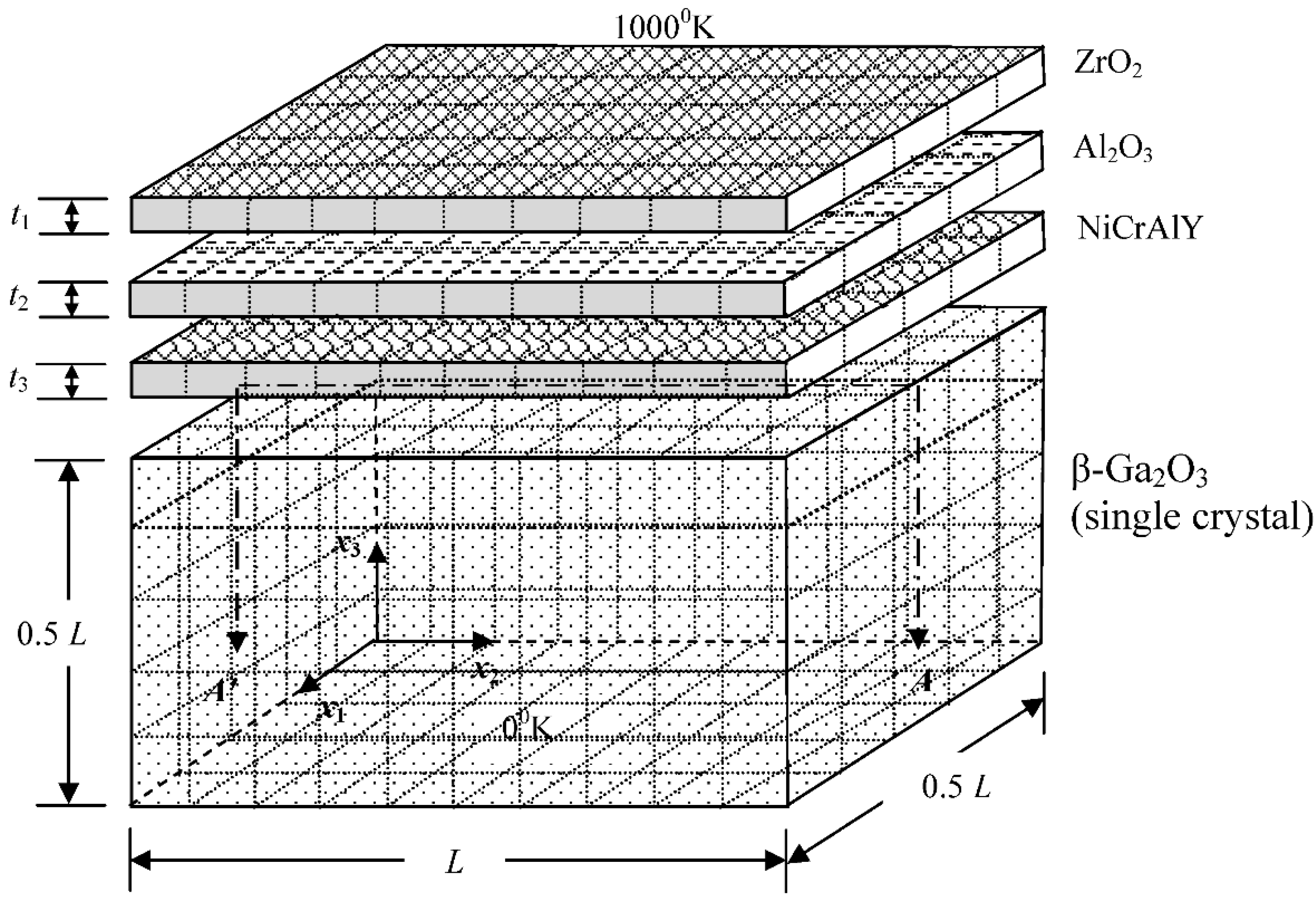
For verifying the approach of our implemented code, the next example treated a typical coated system, as shown in
Figure 5, where the dimensions of all layers are schematically depicted. This system consisted of three layers on a substrate, namely a thin coating layer ZrO
2 on top, a TGO layer of Al
2O
3, a bond-coat layer of NiCrAlY, plus a single crystal substrate made of β-Ga
2O
3, extensively applied in high power electronics. Distance ratios of the three coating layers were arbitrarily assumed to be:
t1/
L = 10
−3~10
−5,
t2/
L = 10
−2,
t3/
L = 10
−2. The system was subjected to a temperature difference
= 1000 °K with the Dirichlet boundary conditions of 1000 °K and 0 °K prescribed respectively on the top and bottom surface, while the rest of the other surfaces were thermally insulated. As shown in
Figure 5, the analysis was to investigate how the thickness of the top coating layer affected the settled temperature across the mid-section
A-A′ (
x1 = 0.25
L) of the top surface of the substrate.
In practice, the coating layers are extremely thin, such that their properties are usually taken to be isotropic, even though our proposed analysis is applicable to treat 3D general anisotropy. The substrate was considered to have generally anisotropic properties. Conductivity coefficients of the coating layers used for the analysis were as follows: ZrO
2 = 1.7 (W/m °K), Al
2O
3 = 12.2 (W/m °K), NiCrAlY = 22.5 (W/m °K). The substrate β-Ga
2O
3 had the following anisotropic conductivities, defined in its principal axes (denoted by an asterisk in the superscript):
Principal axes of the substrate were successively rotated around the
x3-
x1-
x2 axis by 30°–45°–60° clockwise, yielding the following conductivities in the global Cartesian coordinate system:
Also shown in
Figure 5 is the complete BEM mesh-modeling of the whole system, taking only 640 isoparametric quadratic elements with 2288 nodes (for all three
t1 values), The modeling of ANSYS employed 92,800 Solid226 elements with 391,539 nodes (for
t1/
L = 10
−6). Due to the clustering of elements, the modeling of ANSYS is not shown here. Only three different thicknesses of the top coating layer, that is
t1/
L = 10
−4, 10
−5, 10
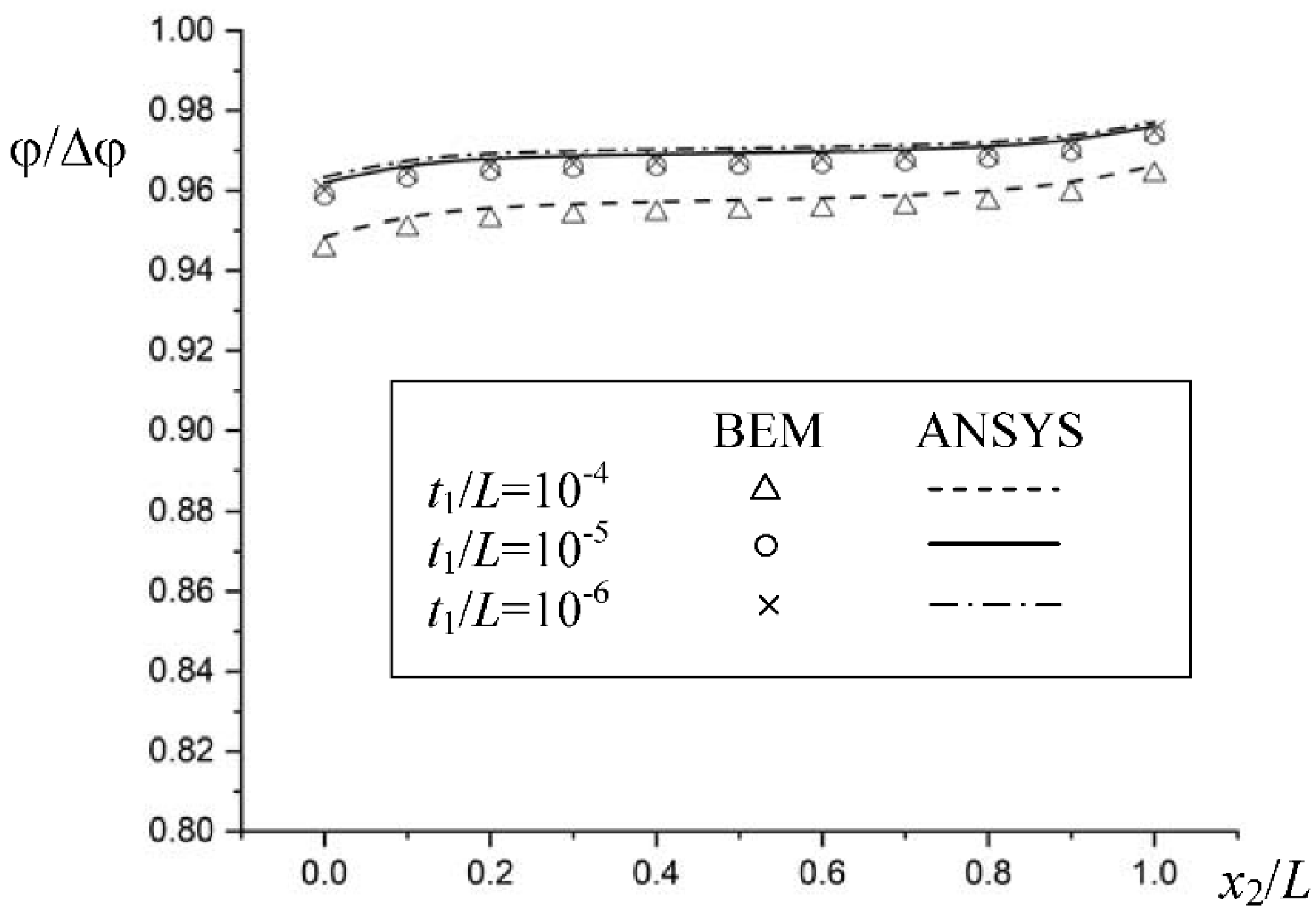
−6, were investigated, although smaller thicknesses could still be modeled by the BEM. The analysis was not carried out for much smaller thicknesses, because the finite element modeling would fail to model the problem, due to the constraint of the elements’ aspect ratio. For comparison of the present analyses, distributions of the settled temperature along
A-
A′ by both analyses were plotted in
Figure 6.
As can be observed from the comparison in
Figure 6, fairly satisfactory agreement between both analyses was present. It should be noted that this study was only to show the veracity of our BEM analysis. The temperature drop across the coating layers was not significant because all side surfaces were insulated and all heat fluxes were allowed to transfer only downward to the substrate. After all, having validated our BEM modeling, the proposed approach is indeed an appealing modeling technique for analyzing the heat conduction problem across thin-coating layers.


