Study on the Characteristics of Boundary Layer Flow under the Influence of Surface Microstructure

Abstract

The energy consumption of a vehicle is closely related to the resistance it receives, and it is of great significance to study the drag reduction of a vehicle to promote energy conservation and emissions reductions. Boundary layer control drag reduction is mainly achieved by controlling the coherent structure in turbulence and reducing its burst intensity and frequency. It can be divided into an active control drag reduction and passive control drag reduction. In passive drag reduction, the advantages of the surface groove drag reduction are relatively obvious. In this paper, the large eddy simulation method is used to study the boundary layer flow with triangular groove and rectangular groove plates along the flow direction under subsonic flow, and to explore the influence of a surface micro-groove structure on the boundary layer flow. The simulation results show that the fluid inside the groove can be blocked by the triangular groove which can keep the low-velocity fluid at the bottom of the groove, and that it can increase the thickness of the viscous bottom layer as well as reduce the velocity gradient at the wall. The spanwise stress component of the Reynolds stress in the triangular groove boundary layer and the burst of turbulence on the wall are inhibited, and the spanwise flow in the boundary layer is blocked. In the subsonic range, about 10% shear force can be reduced because there are secondary vortices induced by the upper flow vortices at the top of the groove wall, and these secondary vortices can restrain the rising of the low-speed strip in the groove and reduce the burst of turbulence. The rectangular groove creates a weak blocking effect on the fluid inside the groove, which can only inhibit spanwise pulsation under subsonic speed. The wall shear stress cannot be reduced when the flow velocity is low, and it even increases.

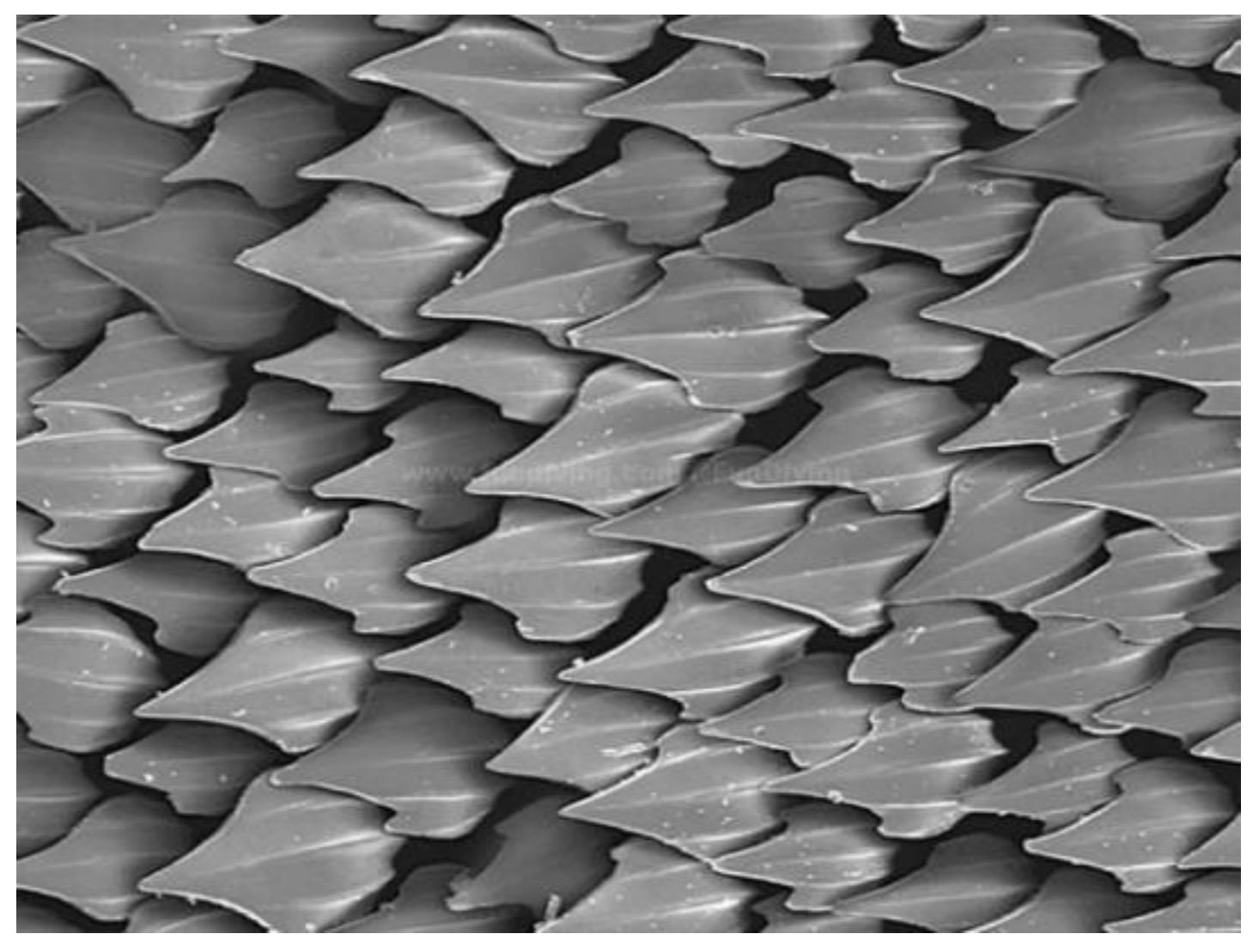
1. Introduction

From the submarine in the water to the ship on the water, and then to the aircraft in the air, resistance has a great impact on the energy consumption of a vehicle. Therefore, in the ship, automobile, aerospace and other fields, vehicle drag reduction is always a very important research direction. In the aerospace field, a large part of the resistance encountered by an aircraft during flight is friction resistance. More than 50% of the total resistance of modern large commercial aircraft is caused by friction [1], and the existence of friction resistance greatly reduces the energy efficiency of aircraft. Using appropriate drag control technology to reduce the flight resistance of aircraft is a key technical approach to improve the ratio of the flight fuel consumption of aircraft under the condition of a limited fuel capacity.

The burst of coherent structures in wall turbulence is the root cause of wall friction resistance, and controlling the coherent structures in turbulence (bands, streamwise vortices, turbulent laminar fluidization, etc.) [2] is a necessary means of drag reduction. The control of turbulent coherent structures can be divided into passive control (wall groove, flexible wall, etc.) and active control (vibrating wall, microbubble method, etc.) according to whether additional energy, momentum, or mass input is needed [3,4].

As far as passive drag reduction is concerned, the surface groove method has more obvious advantages in drag reduction. It is easy to realize, and a groove thin film can be pasted on the surface of the object or a groove structure can be processed on the surface. The drag reduction of surface grooves is derived from the imitation of organisms, and among them the surface microstructure represented by the shark is the most representative. In the 1970s, the Langley Research Center in the United States found that the shark skin surface was not smooth, but was composed of many fine placoid scale structures arranged according to certain rules, forming a groove structure along the flow direction, as shown in Figure 1 (1 cm in the picture corresponds to the actual 100 $\mathsf{\mu }\mathrm{m}$). Because of the existence of these micro-grooves, the frictional drag of sharks when swimming is greatly reduced [5].

With the development of surface micro-structure drag reduction technology, the groove micro-structure has been applied to various fields. Airbus once deployed a micro-grooved structure on Airbus A320 aircraft, which covered 66% of the total area of the aircraft. The test results showed that when the cruising speed of the aircraft was 0.7 Ma, the resistance of the aircraft was reduced by 4.85%, and it achieved the effect of saving 1~2% of fuel. [6]; however, wall grooves usually have a fixed geometry and can only be effective within a limited range of parameters. Outside of the operating range, they can even increase wall friction, having the opposite effect. Although the small groove structure is conducive to inhibiting the transverse migration of streamwise vortexes in the viscous bottom, the mechanism of the groove structure impeding the translation of vortexes and the interaction between grooves is very complex and has not been clearly understood [7]. Therefore, it is necessary to study the boundary layer flow characteristics under the influence of microstructures such as wall grooves as it will provide fundamental data support for the aircraft boundary layer control drag reduction technology.

Surface micro-groove drag reduction is a passive drag reduction method that does not require additional equipment and energy consumption and does not require the addition of other substances to change the composition of the fluid. This method only achieves the purpose of drag reduction by changing the geometric shape of the surface, and the method is simple and effective. As people change the perception that smooth surfaces can reduce friction resistance, more research is being completed on the drag reduction of surface micro-grooves.

Walsh et al. [8,9,10,11] studied the micro-groove extending in the direction of flow and found that micro-grooves can effectively reduce the surfaces of friction resistance, when the groove cross-section shape for the triangle and the groove width of dimensionless s⁺ and the groove equals the dimensionless height h⁺, and that this groove structure was best to reduce the friction resistance effect by 8%. Bacher and Smith [12] calculated a net drag reduction rate of 25% for grooved structures by using the boundary layer momentum integral formula. Gallagher and Thomas [13] studied the drag reduction problem of groove and according to the calculation results of the momentum integral formula of the boundary layer, they found that the total resistance of the groove plate was unchanged, but the resistance of the latter half of the groove plate was reduced. D.W. Bechert [14] conducted wind tunnel experiments and oil channel experiments on three-dimensional groove structures, and the experimental results showed that the turbulent shear stress decreased by about 7.3%, a slightly less than 10% drag reduction for two-dimensional lateral trenches. Park and Wallance [15] measured the velocity distribution in the groove with a hot-wire anemometer and calculated the drag was reduced by 4%. Gaudet [16] studied the turbulent boundary layer of a groove structure at Ma = 1.2 and obtained the drag reduction rate of 7%. Coustols and Cousteix [17] arranged micro-grooves on the suction surface of the LC100D airfoil and measured when the airfoil angle of attack was 0° and 2°, where the total resistance decreased by about 2%, while the viscous friction resistance decreased by 7%. As the angle of attack continued to increase, the results showed no drag reduction effect. Sundaram et al. [18,19] arranged the micro-groove structure on the suction surface and pressure surface of NACA0012 and GAW-2, respectively, and conducted experiments with the wake measurement method, finding that the drag reduction rate was up to 10%. Launder [20] studied channel flows with knife-shaped, triangular, and U-shaped grooves through numerical calculation. By comparing the flow parameters of different grooves, he found that the triangular grooves had the best drag reduction effect, and the drag reduction effect at the dimensionless height of grooves h⁺ > 15 was better than the experimental observation results. Caram and Ahmed [21] arranged the groove structure on the NACA0012 airfoil and measured the flow in the wake area of the airfoil at a zero angle of attack. When the groove height was 0.152 mm, the drag was reduced by 13.3%; when the groove height was 0.076 mm and 0.023 mm, the drag was reduced by 2.7% and 7.3%, respectively. McLean [22] arranged grooves on T-33 wings, and the experimental results showed that when the Mach number was between 0.45 and 0.7, the drag was reduced by 6%. Debisschop and Nieuwstadt [23] studied the flow of groove plates under the influence of an adverse pressure gradient, and found that the drag reduction effect of the groove plate increased due to the influence of the adverse pressure gradient, and its drag reduction rate reached 13%. The study of Djenidi and Antonia [24] found that the drag reduction effect of grooves was closely related to the distance between grooves. Bhushan [25] conducted an experimental study on the complex shark skin surface and found that the sharkskin surface structure could effectively reduce resistance. Douglas and George [26] found that the resistance of the transition zone and turbulence zone was significantly reduced in the numerical simulation of the groove structure in the pipeline. Yulia and Pierre [27] conducted a large eddy simulation of the trench structure arranged along the sinusoidal curve and found that the drag reduction effect of the arrangement was better than that of the arrangement along the straight line.

Compared with foreign countries, the research on the drag reduction of surface micro-grooves in China started late, but some achievements have been made. Shi Xiu-hua and Fu Hui-ping et al. [28] from Northwestern Polytechnical University studied the drag reduction performance of surface micro-grooves by combining a numerical simulation with a flume experiment and found when the apex angle of triangular grooves was 60°, their drag would be reduced by about 11%. Du Jian [29] used the method of combining a numerical simulation and wind tunnel experiment verification to study the drag reduction of surface microscopic grooves, and the results showed that the frictional resistance was reduced in areas other than the tip of the groove, which was analyzed to be because the existence of grooves affected the turbulent flow of the incoming flow and blocked the instantaneous transverse movement of the turbulent flow. Wang Jin-jun [30] studied the turbulent ordered structure of grooves, studied the drag reduction mechanism of surface micro-grooves, and carried out experimental verification by a wind tunnel. Cong Qian et al. [31,32] numerically simulated the flow field of triangular, fan-shaped, and knife-shaped grooves by using the finite volume method, and carried out experimental verification in a wind tunnel, which showed that triangular, fan-shaped, and knife-shaped grooves could reduce friction resistance by 3%, 9%, and 10%, respectively. Zhang Xiao-ci et al. [33] theoretically analyzed the possibility of transverse microscopic grooves reducing frictional resistance according to the Karman vortex street resistance formula and analyzed the geometric shape of a vortex street traveling wave. Li Yu-bin et al. [34] arranged micro-groove structures on the surface of the yun7 model and measured that aircraft resistance decreased by about 5~8%. Song Bao-wei et al. [35] concluded that the effect of traveling wave resistance would decrease with the increase of flow velocity by studying the surface of micro-grooves. Hu Hai et al. [36] carried out a wind tunnel experiment and water tunnel experiment, respectively, on a cyclotron with groove structures. It was found that the groove structures had a stable drag reduction effect when the angle of attack was not large, and the drag reduction rate was up to 6%. Zhang bin and Chang Yue-feng et al. [37,38] used an IFA300 constant temperature hot-wire anemometer to measure the instantaneous velocity of a turbulent boundary layer on smooth plate and triangular groove surfaces under different incoming flow velocities and zero pressure gradients in low-speed wind tunnel experiments. The analysis showed that the triangular grooves reduced the friction resistance by changing the flow structures of different scales in the turbulent boundary layer. Huang Zhi-ping [39] and Sun Peng-xiang [40] conducted water tunnel experiments on a shark skin surface structure and found that the drag reduction effect of the shark skin surface could reach 18.6%. Zhao Zhi-yong et al. [41] found that the drag reduction effect of grooves was related to the curvature of the groove tip, while the research results of Liu Zhan-yi et al. [42] showed that the ratio of groove spacing to groove height has a great influence on the drag reduction effect.

Based on the large eddy simulation (LES) technique, the numerical simulation method was used to study the influence of surface grooves with different cross-section shapes on the characteristic parameters of the boundary layer at different incoming flow velocities.

2. Physical Model and Numerical Method

2.1. LES Method

Large eddy simulation (LES) is a turbulence simulation method between direct numerical simulation (DNS) and Reynolds-averaged Navier–Stokes (RANS). LES directly simulates the mass, momentum, and energy of the large-scale eddies, while the effect of the small-scale eddies on the large-scale eddies is simulated through modeling.

There are two key processes in LES. The first is the filtration process. The function of filtration is to filter out the small-scale vortices below the filtration scale and directly solve the vortices above the filtration scale. For the small-scale vortex below the filter scale, a mathematical model is established to simulate it. After filtering, an additional stress term will appear in the governing equation, which is called subgrid stress, which reflects the effect of the small-scale vortex on the large-scale vortex. The simulation of the small-scale vortex is to establish an appropriate subgrid stress model.

The filtering of LES is to decompose the physical quantity into the quantity that can be solved directly and the scale quantity that cannot be solved directly. The mathematical expression is as follows:

$$\varphi \left(x,t\right)=\overline{\varphi }\left(x,t\right)+{\varphi }^{\prime }\left(x,t\right)$$

(1)

The solvable scale quantity is defined by the convolution integral of the flow variable $\varphi \left(x,t\right)$:

$$\overline{\varphi }\left(x,t\right)={\iiint }_{\Omega }G\left(x-x^{\prime },\Delta \right)\varphi \left(x,t\right)d{x}^{\prime }d{y}^{\prime }d{z}^{\prime }$$

(2)

In Equation (2) $\varphi \left(x,t\right)$ is an arbitrary physical quantity in a flow fild, $\overline{\varphi }\left(x,t\right)$ is a solvable scale quantity, and ${\varphi }^{\prime }\left(x,t\right)$ is an unsolvable scale quantity. $G\left(x-x^{\prime },\Delta \right)$is a spatial filter function, which determines the size and structure of the small-scale vortex, and δ is the filter scale. Equation (2) is the filtering operation. Vortices above $\Delta$are regarded as large vortices and solved directly, while vortices below $\Delta$ are not solved directly but simulated by a sub-lattice model. The filter scale $\Delta$ is not necessarily related to the grid size at the time of calculation, but it is generally regarded as a function of grid resolution.

$$\Delta ={(\Delta x\Delta y\Delta z)}^{\frac{1}{3}}$$

(3)

In Equation (3), $\Delta x$, $\Delta y$ and $\Delta z$ are grid dimensions in x, y and z directions, respectively.

For incompressible fluid, the governing equation after filtration operation is as follows:

Continuity equation

$$\frac{\partial {\overline{u}}_j}{\partial x_j}=0$$

(4)

Momentum equation:

$$\frac{\partial {\overline{u}}_i}{\partial t}+{\overline{u}}_j\frac{\partial {\overline{u}}_i}{\partial x_j}=\overline{f}-\frac{1}{\rho }\frac{\partial \overline{p}}{\partial x_i}+\frac{1}{\rho }\frac{\partial }{\partial x_i}\left({\overline{\tau }}_{ji}+{\tau }_{jiSGS}\right)$$

(5)

In Equation (5):

$$\overline{{\tau }_{ji}}=\mu \left(\frac{\partial {\overline{u}}_i}{\partial x_j}+\frac{\partial {\overline{u}}_j}{\partial x_i}\right)$$

(6)

$${\tau }_{jiSGS}=-\rho \left(\overline{u_i{u}_j}-\overline{u_i}\overline{u_j}\right)$$

(7)

Energy equation:

$$\frac{\partial \overline{T}}{\partial t}+{\overline{u}}_j\frac{\partial \overline{T}}{\partial x_j}=\frac{1}{\rho c_p}\frac{\partial }{\partial x_j}\left(-{\overline{q}}_j+q_{j,SGS}\right)$$

(8)

In Equation (8):

$${\overline{q}}_j=-k\frac{\partial \overline{T}}{\partial x_j}$$

(9)

$$q_{j,SGS}=-\rho \left(\overline{u_{j}T}-{\overline{u}}_j\overline{T}\right)$$

(10)

where ${\tau }_{jiSGS}$ is the subgrid turbulent stress; $q_{j,SGS}$ is the heat flux of subgrid.

Another part of the subgrid stress model is based on the assumption of eddy viscosity to calculate the eddy viscosity coefficient. The eddy-viscous model of the subgrid turbulent stress is:

$${\tau }_{jiSGS}-\frac{1}{3}{\tau }_{kk,SGS}{\delta }_{ij}=2{\mu }_{SGS}{\overline{s}}_{ij}$$

(11)

where ${\mu }_{SGS}$ is the subgrid eddy viscosity coefficient. It can be calculated using the Smagorinsky model with fixed model coefficients.

The Smagorinsky model was proposed by J. Smagorinsky in 1963, and its model is:

$${\mu }_{SGS}=\rho {(C_s\Delta )}^2\left|\overline{s}\right|$$

(12)

In Equation (12):

$$\overline{s}=\sqrt{2{\overline{s}}_{ij}{\overline{s}}_{ij}}$$

(13)

$${\overline{s}}_{ij}=\frac{1}{2}\left(\frac{\partial {\overline{u}}_i}{\partial x_j}+\frac{\partial {\overline{u}}_j}{\partial x_i}\right)$$

(14)

where $C_s$ is the Smagorinsky constant, and its value range is usually 0.1~0.2.

The anisotropy of turbulent flow needs to be considered in the near-wall region ${\mu }_{SGS}$, and the most widely used method is to use the damping function $D_s$ to correct the Smagorinsky constant $C_s$, namely:

$${\mu }_{SGS}=\rho {(C_s{D}_s\Delta )}^2\left|\overline{s}\right|$$

(15)

The damping function $D_s$ is:

$$D_s=1-e^{-\left(y^{+}/A^{+}\right)}$$

(16)

where y⁺ is the dimensionless distance from the wall; A⁺ is an empirical constant.

The selection of Smagorinsky constant $C_s$ has a great influence on the calculation results of the large eddy simulation. A larger $C_s$ can obtain a smooth changing spatial structure in turbulent simulation, but too large a $C_s$ will cause the motion of large-scale eddies to be attenuated and cause calculation errors. Smaller $C_s$ can obtain excellent results in turbulent flow with heat conduction and the turbulent boundary layer, but because $C_s$ has a great influence on the pulsation speed, too small a $C_s$ can cause pulsation in the simulation results.

The subgrid heat flux $q_{j,SGS}$ adopts the gradient diffusion model:

$$q_{j,SGS}=-\rho c_p\left(\overline{u_{j}T}-{\overline{u}}_j\overline{T}\right)=k_{SGS}\frac{\partial \overline{T}}{\partial x_j}=\frac{{\mu }_{SGS}{c}_p}{P{r}_{SGS}}\frac{\partial \overline{T}}{\partial x_j}$$

(17)

where $P{r}_{SGS}$ is the subgrid Prandtl number, and its value is about 0.9; $k_{SGS}$ is the subgrid thermal conductivity.

For compressible fluids, many unknown terms will be generated in the governing equations due to density fluctuations. To avoid this problem, Favre filtering is used when filtering the governing equations of compressible fluids.

The governing equation after Favre filtering operation is as follows:

Continuity equation:

$$\frac{\partial \overline{\rho }}{\partial t}+\frac{\partial \overline{\rho }{\tilde{u}}_j}{\partial x_j}=0$$

(18)

Momentum equation:

$$\frac{\partial \overline{\rho }{\tilde{u}}_i}{\partial t}+\frac{\partial \overline{\rho }{\tilde{u}}_j{\tilde{u}}_i}{\partial x_j}=\overline{\rho }{\overline{f}}_t-\frac{\partial \overline{p}}{\partial x_i}+\frac{\partial {\overline{\tau }}_{ij}}{\partial x_j}+\frac{\partial }{\partial x_j}\left[-\overline{\rho }\left(\widetilde{u_j{u}_i}-{\tilde{u}}_j{\tilde{u}}_i\right)\right]+\frac{\partial }{\partial x_i}\left({\overline{\tau }}_{ji}-{\tilde{\tau }}_{ji}\right)$$

(19)

In Equation (12):

$${\tilde{\tau }}_{ji}=-\frac{2}{3}\mu \left(\tilde{T}\right)\frac{\partial {\tilde{u}}_k}{\partial x_k}+2\mu \left(\tilde{T}\right)\left(\frac{\partial {\tilde{u}}_i}{\partial x_j}+\frac{\partial {\tilde{u}}_j}{\partial x_i}\right)$$

(20)

$${\tau }_{ij,SGS}=-\overline{\rho }\left(\widetilde{u_j{u}_i}-{\tilde{u}}_j{\tilde{u}}_i\right)$$

(21)

where $\frac{\partial {\tau }_{ij,SGS}}{\partial x_j}$ is the subgrid turbulence stress, $\frac{\partial }{\partial x_i}\left({\overline{\tau }}_{ji}-{\tilde{\tau }}_{ji}\right)$ is the subgrid viscous stress, and this is caused by the nonlinear viscous stress.

Energy equation:

$$\begin{gathered} \frac{\partial \overline{\rho }\tilde{E}}{\partial t}+\frac{\partial \overline{\rho }{\tilde{u}}_j\tilde{E}}{\partial x_j}=\overline{\rho }{\overline{f}}_j{\tilde{u}}_j-\frac{\partial \overline{p}{\tilde{u}}_j}{\partial x_j}+\frac{\partial {\overline{\tau }}_{ji}{\tilde{u}}_i}{\partial x_j}+\frac{\partial \left(-{\tilde{q}}_j\right)}{\partial x_j}+S\left(\tilde{T}\right)+ \\ \frac{\partial }{\partial x_i}\left(-\overline{\rho u_{j}E}+\overline{\rho }{\tilde{u}}_j\tilde{E}-\overline{p{u}_j}+\overline{p}{\tilde{u}}_j+\overline{{\tau }_{ji}{u}_i}-{\overline{\tau }}_{ji}{\tilde{u}}_j-{\overline{q}}_j+{\tilde{q}}_j\right) \end{gathered}$$

(22)

In Equation (15):

$${\tilde{q}}_j=-k\left(\tilde{T}\right)\frac{\partial \tilde{T}}{\partial x_j}$$

(23)

The non-closed term of the momentum equation after Favre filtering is mainly the subgrid model turbulent stress. In order to solve this term, a subgrid model needs to be introduced. Here, the Smagorinsky model with fixed coefficients is used, but different from the compressible flow, the subgrid ${\tau }_{kk,SGS}$ needs to be input separately into the model:

$${\tau }_{ji,SGS}-\frac{1}{3}{\tau }_{kk,SGS}{\delta }_{ij}=2C_s^2\overline{\rho }{\Delta }^2\left|\tilde{S}\right|\left({\tilde{S}}_{ij}-\frac{1}{3}{\tilde{S}}_{kk}{\delta }_{ij}\right)=C_s^2{\alpha }_{ij}$$

(24)

$${\tau }_{kk,SGS}=2C_I\overline{\rho }{\Delta }^2{\left|\tilde{S}\right|}^2=C_I\alpha$$

(25)

In the above Equation, $C_s$ = 0.16, $C_I$ = 0.09, $\left|\tilde{s}\right|=\sqrt{2{\tilde{s}}_{ij}{\tilde{s}}_{ij}}$, ${\tilde{s}}_{ij}=\frac{1}{2}\left(\frac{\partial {\tilde{u}}_i}{\partial x_j}+\frac{\partial {\tilde{u}}_j}{\partial x_i}\right)$.

The subgrid heat flux density in the compressible flow also adopts the gradient diffusion model, and the specific form is as follows:

$$Q_j=-C_s^2\frac{{\Delta }^2\overline{\rho }\left|\tilde{S}\right|}{{\mathit{Pr}}_T}\frac{\partial \tilde{T}}{\partial x_i}$$

(26)

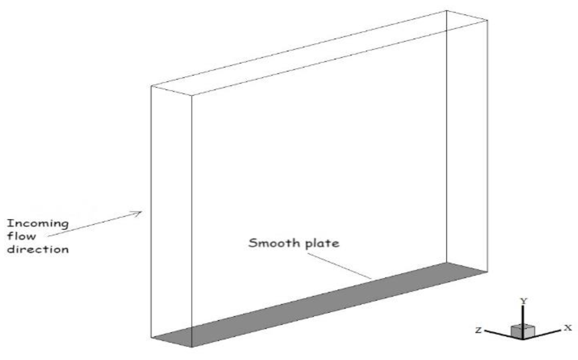
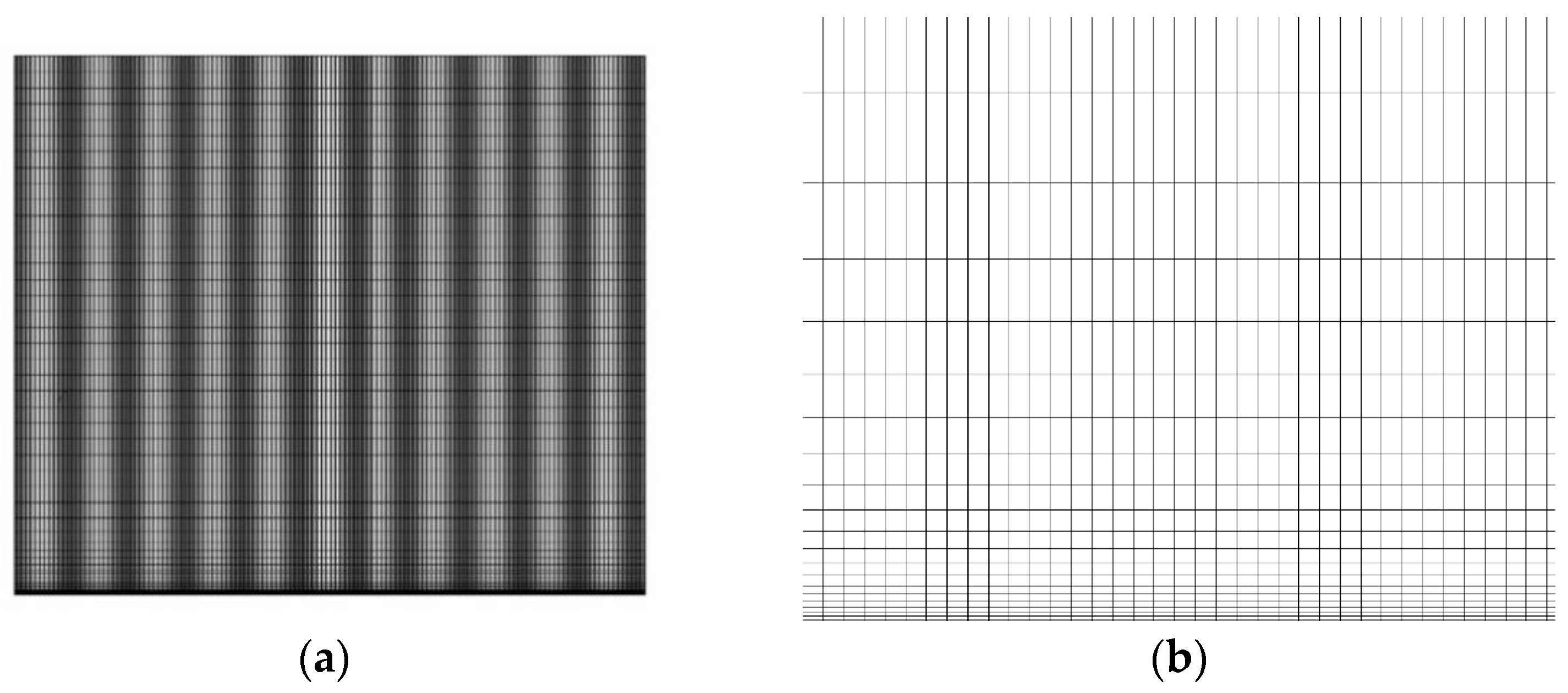
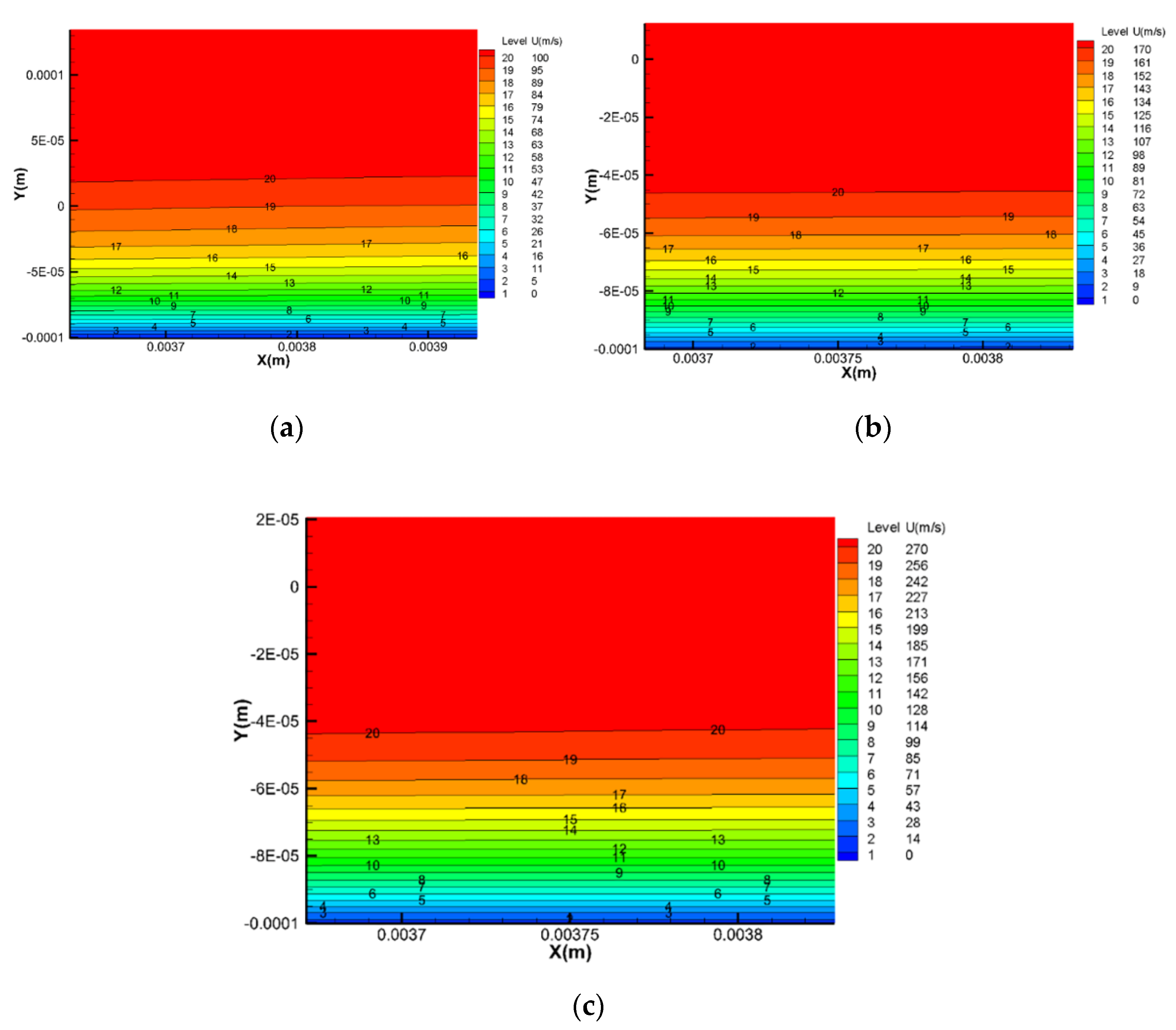
2.2. Smooth Plate Model and Meshing

The span length of the smooth plate is 0.001 m. According to the calculation formula of the boundary layer thickness Equation (27), the maximum thickness of the boundary layer at 0.3 Ma is 0.0003167 m. The wall-normal height of the computing domain is more than 20 times that of the boundary layer, and the normal height of the computing domain is 0.007 m. To ensure the full development of the flow, the spanwise length of the computational domain is also more than 20 times that of the boundary layer, and the streamwise length is 0.0075 m. The computational domain model of the smooth plate is shown in Figure 2.

$$\delta \left(x\right)=0.37x{(\frac{\rho U_{\infty }x}{\mu })}^{-\frac{1}{5}}$$

(27)

For the simulation of turbulent flow in the near-wall region, a sufficiently fine mesh is used to divide the near wall surface, the first layer nodes of the mesh are arranged inside the viscous bottom layer, y⁺ is less than 1, and then LES is used to solve the near wall area in detail. The smooth plate mesh of the flow direction angle is shown in Figure 3.

This paper uses Fluent to perform the numerical simulation calculations, which is a computational fluid dynamics software based on the finite volume method. For the physical characteristics of each flow problem, a numerical solution suitable for it was used to achieve the optimal calculation speed, stability and accuracy.

For the smooth and flat surface flow numerical simulation, the speed range of calculation conditions was from low speed to high subsonic speed. The ambient static temperature was 288.3 k, the air density was ρ = 1.225 kg/m³, and the air viscosity coefficient was μ = 1.78 × 10⁻⁵ Pa·s. The specific parameters are shown in

Table 1. Smooth plate calculation conditions.

Ma	$\mathit{D}\mathit{e}\mathit{n}\mathit{s}\mathit{i}\mathit{t}\mathit{y}$ $\mathit{\rho }$$(\mathbf{k}\mathbf{g}/{\mathbf{m}}^3)$	$\mathit{V}\mathit{i}\mathit{s}\mathit{c}\mathit{o}\mathit{s}\mathit{i}\mathit{t}\mathit{y} \mathit{C}\mathit{o}\mathit{e}\mathit{f}\mathit{f}\mathit{i}\mathit{c}\mathit{i}\mathit{e}\mathit{n}\mathit{t}$ $\mathit{\mu }$$(\mathbf{P}\mathbf{a}\cdot \mathbf{s})$	Static Temperature T (K)	Characteristic Length L (m)
0.1	1.225	1.78 × 10−5	288.3	0.0075
0.3
0.5
0.8

.

The turbulence model required for the calculation selects the LES, and the subgrid model of LES selects the Smagorinsky model regarding the boundary conditions, since the flow is periodic in the flow direction and the span direction, the periodic boundary conditions are adopted in the flow direction and the span direction, the normal boundary of the computational model is physically the surface of the plate, and, therefore, the adiabatic no-slip wall boundary condition is used on the normal boundary. Since the calculation conditions are from low speed to high subsonic speed, considering the convergence problem, the solver chooses the pressure-based couple algorithm. For the selection of the discrete format, considering that the second-order upwind format introduces more upstream nodes, the calculation accuracy is higher, and it has the characteristics of convective transport. Therefore, the second-order upwind format was selected as the discrete format for the convection term.

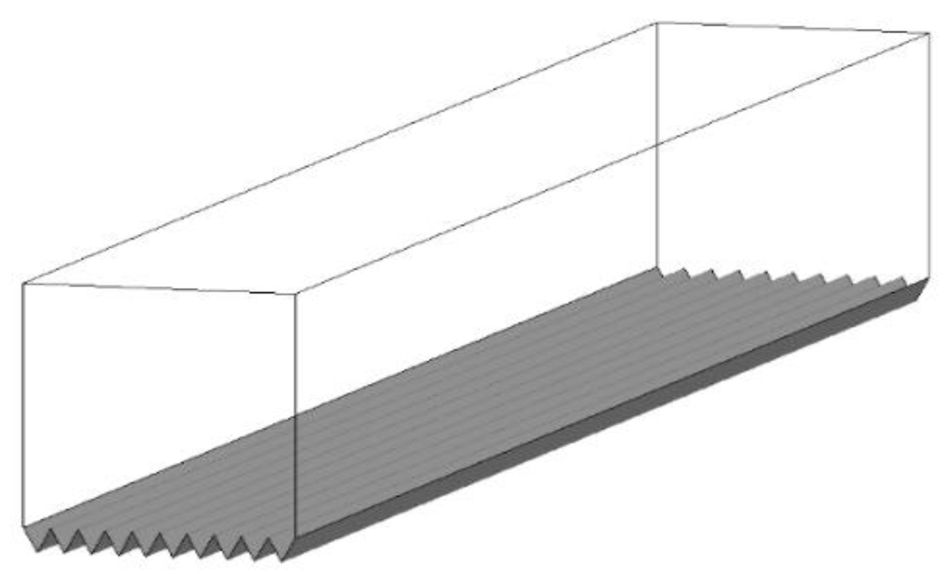
2.3. Surface Microstructure Calculation Model and Meshing

The flow direction length of the plate with grooves was 0.0075 m, the span length was 0.001 m, and the grooves were triangular and rectangular, respectively. The width and depth of triangular grooves were equal and 0.0001 m, so the number of grooves arranged in the span was 10. For rectangular grooves, according to the dimension parameters of triangular grooves, the width of rectangular grooves was 0.00012 m, the height was 0.0001 m, and the number of rectangular grooves arranged in the span was 7. Considering the number of grids and calculation accuracy, the normal height of the plate was 0.001 m.

In order to meet the accuracy requirements of LES on the calculation grid, the number of grids of the calculation model needs to be large enough, but considering the limited performance of the computing equipment, the grids required for the calculation cannot be increased indefinitely. In order to solve the contradiction between the computing power and the number of meshes, while controlling the size of the calculation model as much as possible, a relatively sparse mesh was used far away from the wall surface. However, in order to capture the flow characteristics in the groove and the boundary layer, the near-wall mesh and the inner mesh of the groove were properly refined. LES requires y⁺ < 1 for the nodes of the first layer of the grid, and the y⁺ of the first layer of the grid was set to 0.7, then the height of the first layer of the grid was 0.0017597 mm. Since there are two directions in the normal direction of the wall of the rectangular groove, perpendicular to the plate and along the span direction, therefore the walls in both directions should be set to a first-layer grid height of 0.0017597 mm. Grids of triangular and rectangular grooved surface plates are shown in Figure 4, Figure 5, Figure 6 and Figure 7.

In the setting of boundary conditions, the boundary surface of the flow direction and span direction was set as the periodic boundary condition, and the boundary surface of the groove wall and the upper boundary surface of the computational domain were set as the adiabatic non-slip wall boundary condition.

Because the working condition was at subsonic speed, the pressure-based couple algorithm was chosen to solve the problem. In terms of discrete format, the second-order upwind format was used to solve all equations, and the calculation time step was 0.0001s.

3. Calculation Results and Analysis

3.1. Numerical Method Validation

In order to verify the accuracy of the boundary layer flow, the calculation was based on the large eddy simulation (LES) method in this paper. In the standard atmospheric environment, LES is used to calculate the smooth plate boundary layer flow when the flow velocity is 0.1 Ma and compared with the literature data of Roidl [43]. Considering that the calculation conditions in the following calculation were quite different from those in the literature, it was necessary to further verify the LES. The Reynolds-averaged Navier–Stokes (RANS) and LES method were used to simulate the flow field of the smooth plate at different speeds. The comparison between the results and the theoretical calculation results was carried out to verify the applicability of the method in this paper under different working conditions.

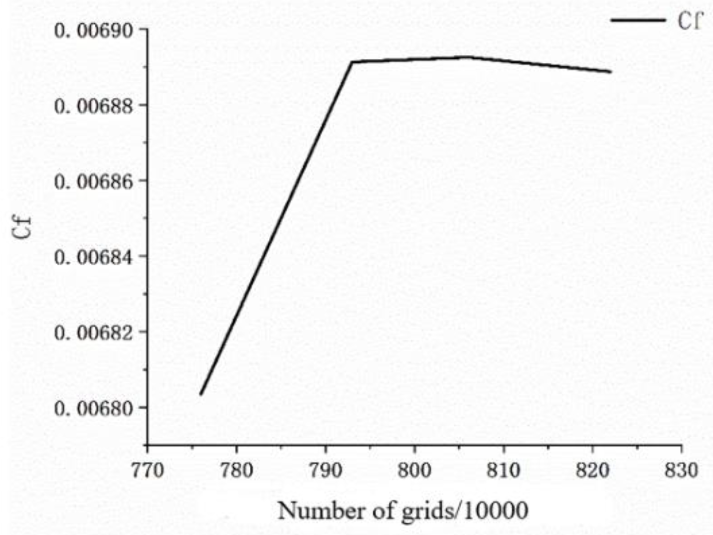
3.1.1. Grid Independence Verification of Smooth Plate

LES has a high requirement for computational grids. To meet the requirements of computational accuracy and reduce the number of grids as much as possible, it is necessary to verify the independence of grids. For the smooth plate, four mesh numbers of 2.99 million, 3.44 million, 3.83 million, and 4.26 million were selected to calculate the frictional drag coefficient of the smooth plate at 0.1 Ma.

Figure 8 can be found when the number of grids was above 3.83 million, and the friction drag coefficient basically did not change. It can be confirmed that the calculation accuracy could only be satisfied when the calculation grid of the smooth plate model in this paper was at least 3.83 million. Therefore, the number of grids of the smooth plate was 3.83 million.

3.1.2. Comparative Analysis of Literature Results

Figure 9 shows the comparison between the calculated results in this paper and the results in the literature at 0.1 Ma. The comparison parameter is the friction drag coefficient, and the calculation result was taken from the straight line along the flow direction at the half span of the smooth plate. It can be seen from the figure that the calculation results of the LES in this paper were between the results of the RANS and LES provided in the literature. There was an error between the calculation results of this paper and the LES results of the literature, and the main analysis error is due to the precision of the discrete format of the terms.

Figure 10 is the comparison between the calculated results of the velocity profile of the smooth plate and the results of the literature at 0.1 Ma.

The above comparison shows that the gap between the simulation results and the literature results was small, so the LES method was suitable for the calculation in this paper.

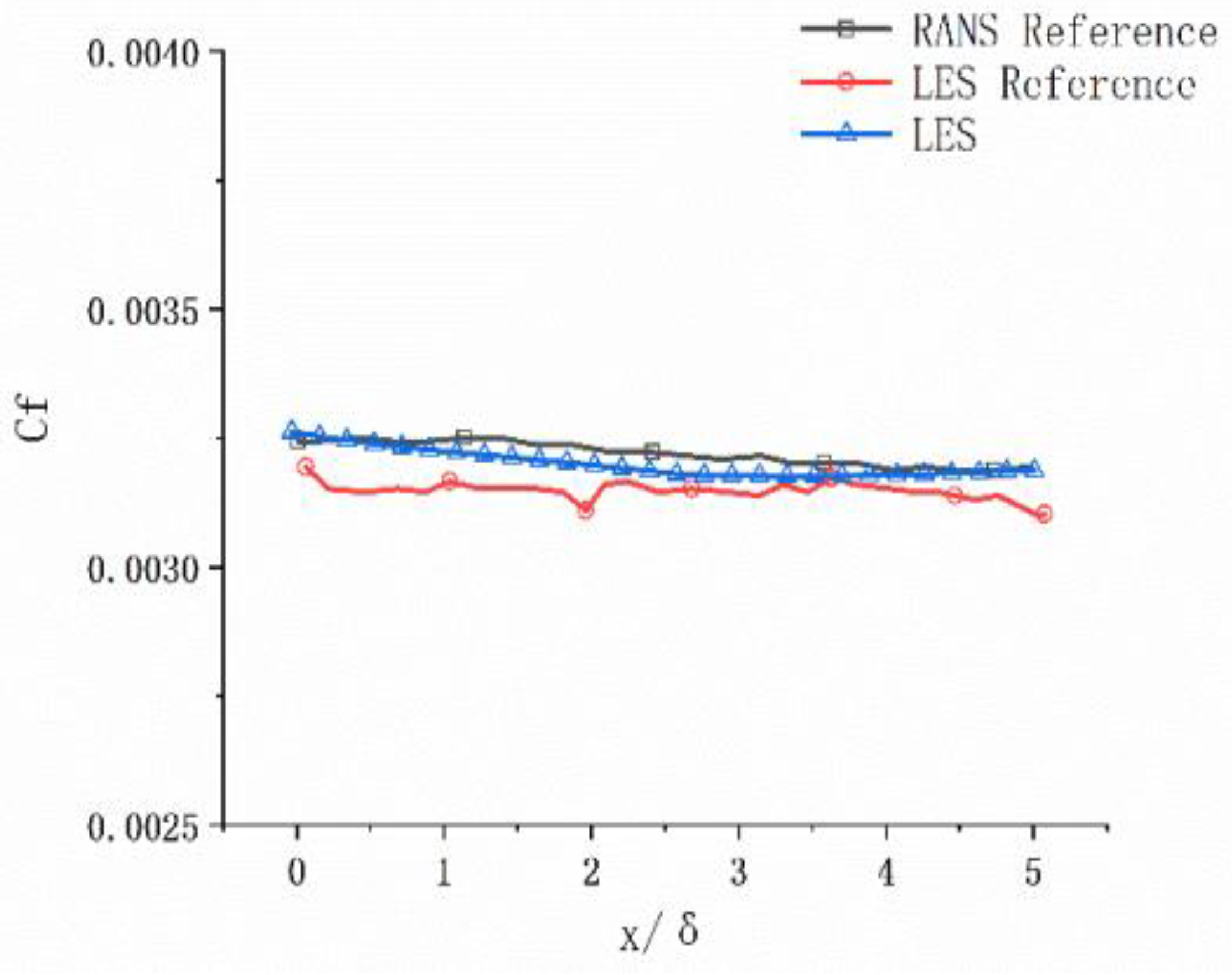
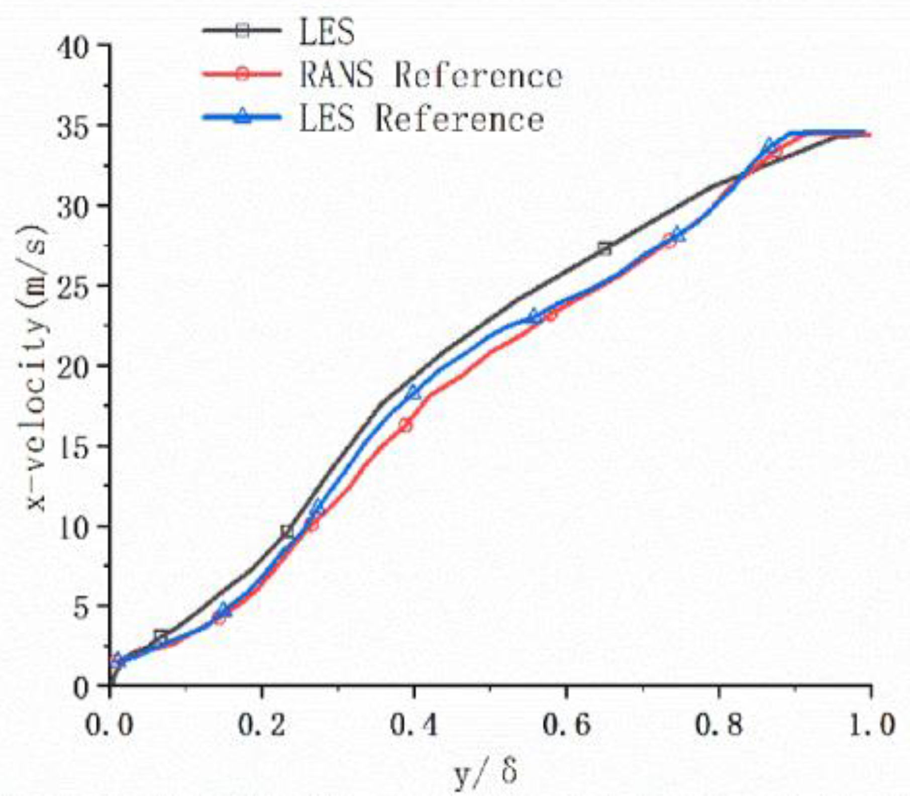
3.1.3. Comparison of the Results of LES and RANS

Considering that the calculation conditions in the following calculation were quite different from those in the literature, it was necessary to further verify the LES. RANS and LES were used to simulate the flow field of the smooth plate at different speeds. The comparison between the results and the theoretical calculation results was carried out to verify the applicability of the method in this paper under different working conditions.

Figure 11a–c, respectively, show the distribution of frictional drag coefficient in the flow direction calculated by the LES and RANS at the spanwise z = 0.0005 m of the smooth plate at different speeds. The horizontal axis adopts dimensionless units, and δ is the thickness of the boundary layer calculated according to Equation (27). It can be seen from the figures that the frictional drag coefficient distributions calculated by the LES and RANS were well fitted.

Table 2. Frictional drag coefficient of smooth plate.

Ma	Re	Cf-Les	Cf-Rans	Cf-Theory
0.3	52647.47	0.00799	0.00906	0.00845
0.5	87745.79	0.00727	0.00807	0.0076
0.8	140393.3	0.00665	0.00655	0.00691

shows the frictional drag coefficients of the smooth plate at different Reynolds numbers, which was calculated by LES, RANS and the theoretical formula, respectively. It can be seen that the calculation results by LES were closer to the theoretical value. The above calculation results further illustrate the accuracy of the LES method.

3.2. Large Eddy Simulation of Plate Boundary Layer under Subsonic Flow

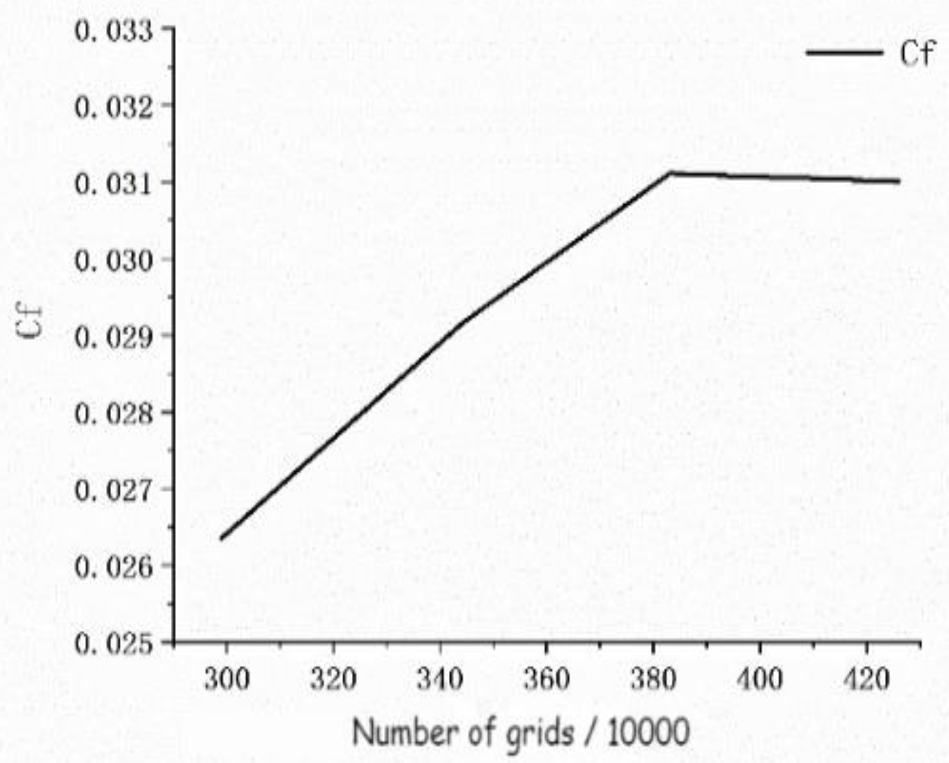
3.2.1. Grid Independence Verification

Considering that the grooved plate was similar in structure, the triangular groove plate was taken for grid independence verification. The meshes of the triangular groove plate were 7.76 million, 7.93 million, 8.06 million, and 8.22 million, respectively, and were calculated in the standard atmospheric environment with a Mach number Ma = 0.8.

Figure 12 shows the variation of the frictional drag coefficient of the triangular groove plate with the number of meshes in the computational domain at 0.8 Ma. It can be seen from the figure that after the number of grids reached 7.93 million, the frictional drag coefficient tended to be stable with the increase of the number of grids, so it can be determined that the calculation requirements were met when the number of grids was 7.93 million.

For the triangular groove plate, the nodes were arranged in the form of 512 nodes in the flow direction, 42 nodes in the normal direction excluding the grooves, and 30 nodes on each triangular hypotenuse inside the grooves in the spanwise direction. A similar arrangement was used for the rectangular groove plate, resulting in a final mesh count of 7.97 million.

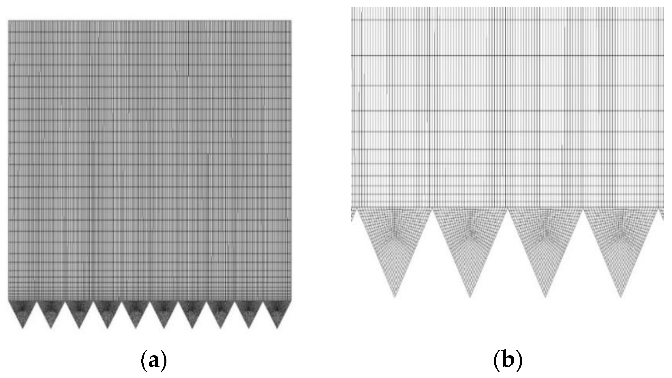
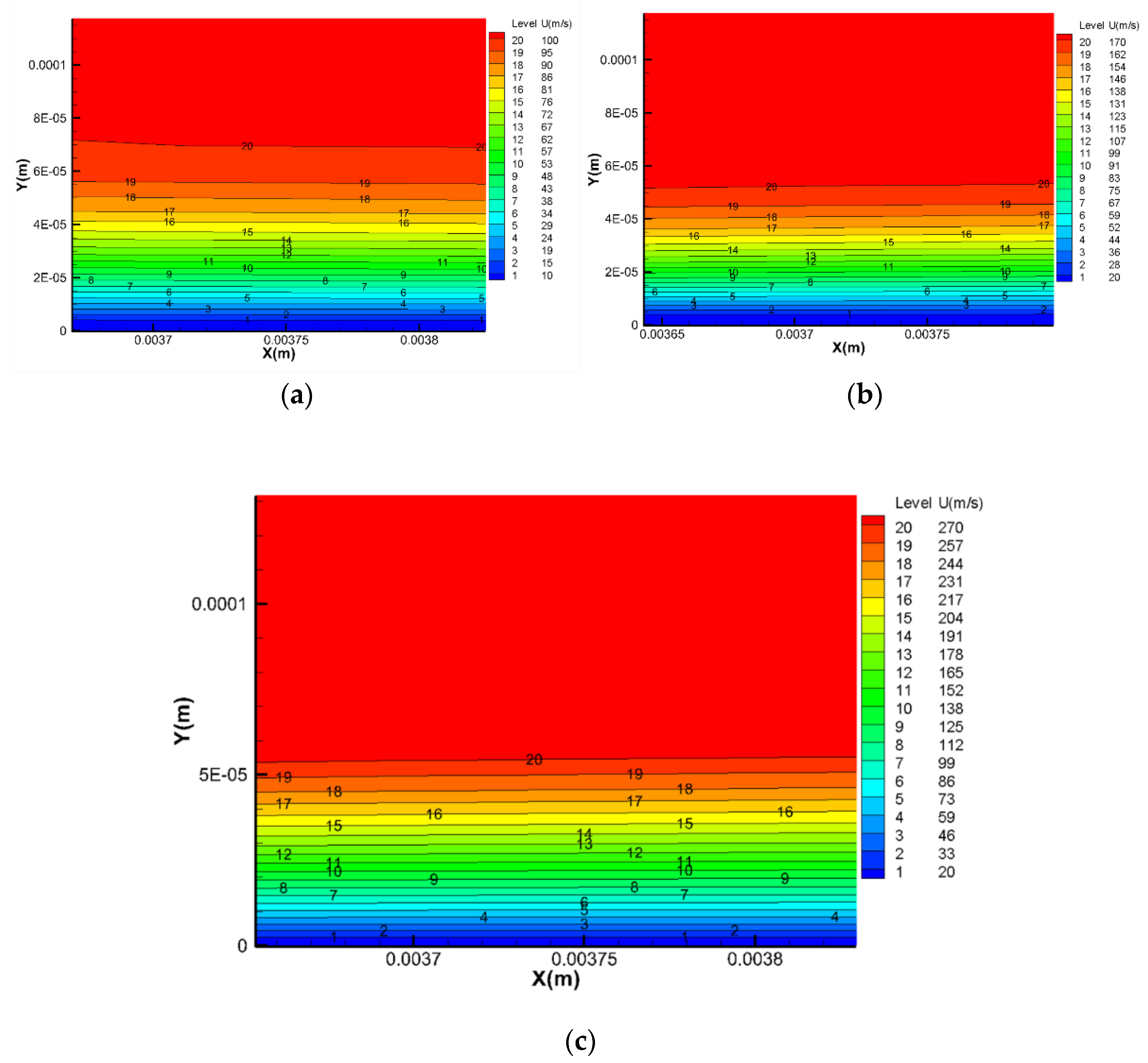
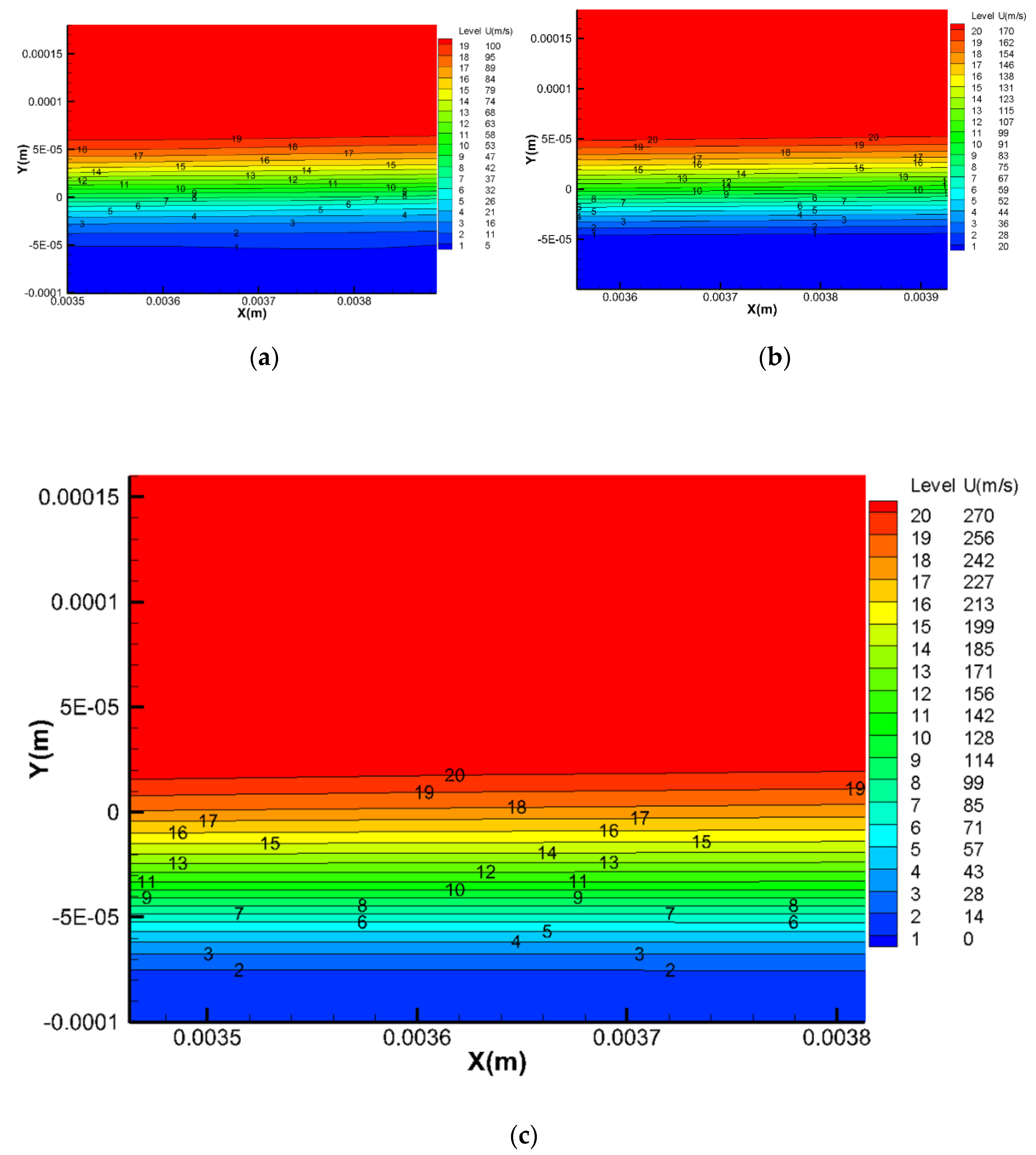
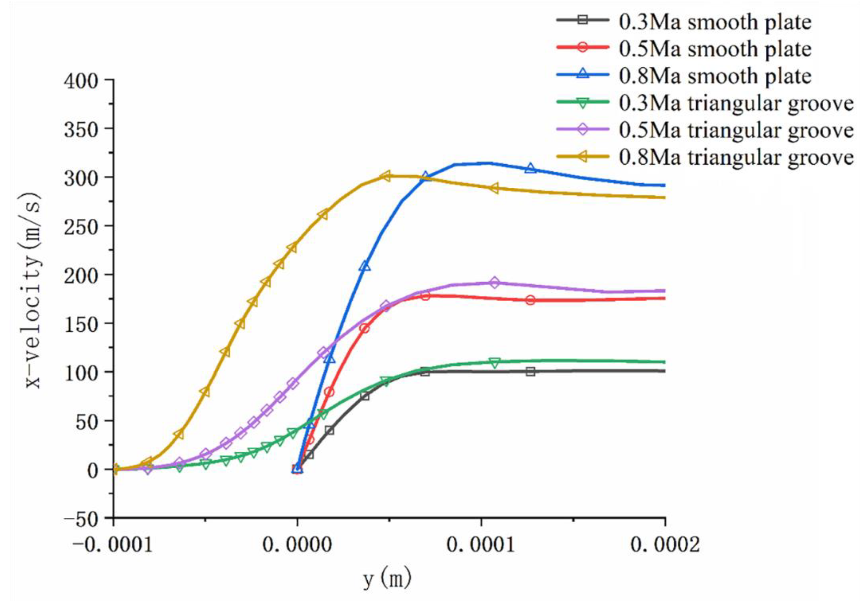
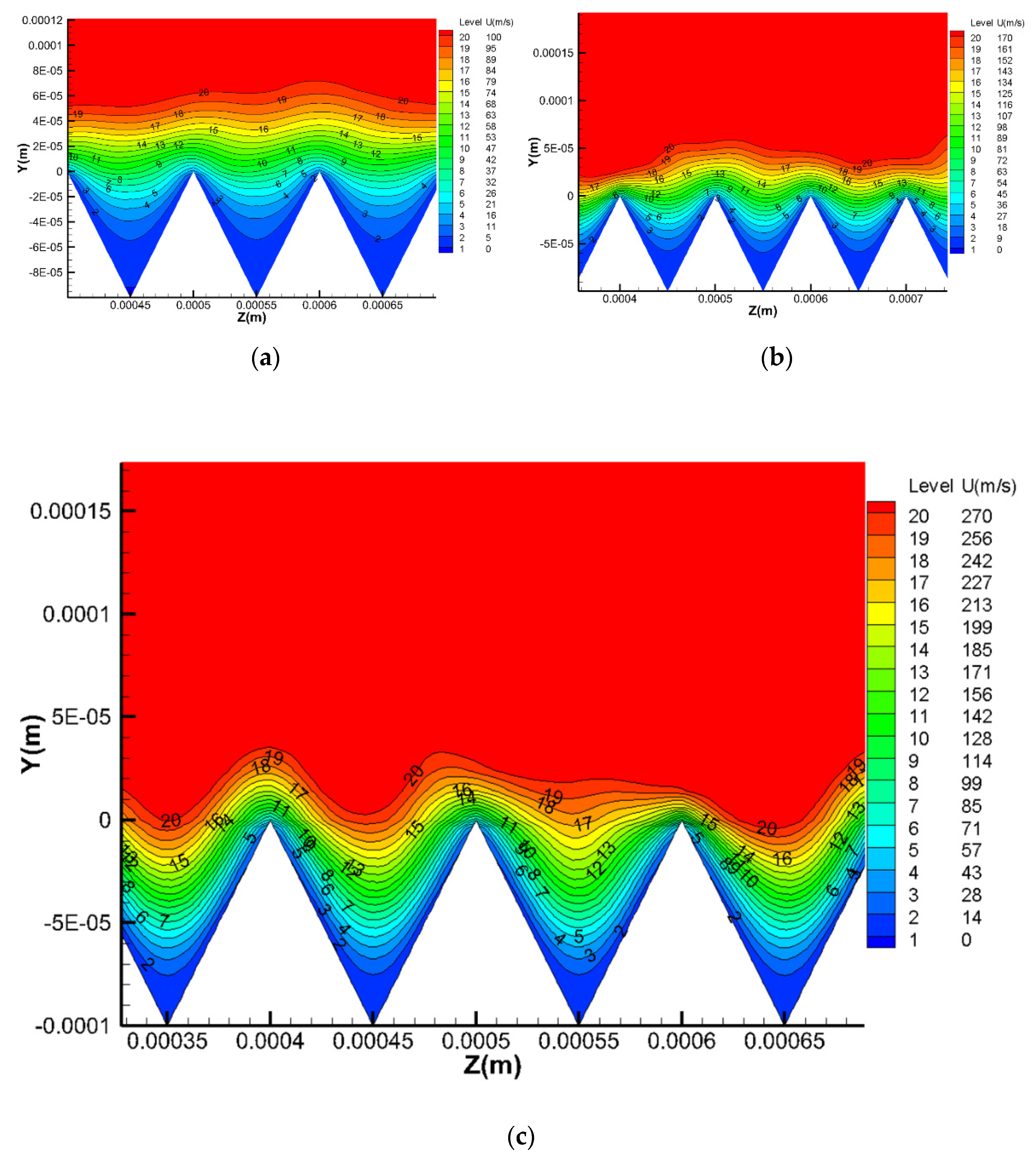
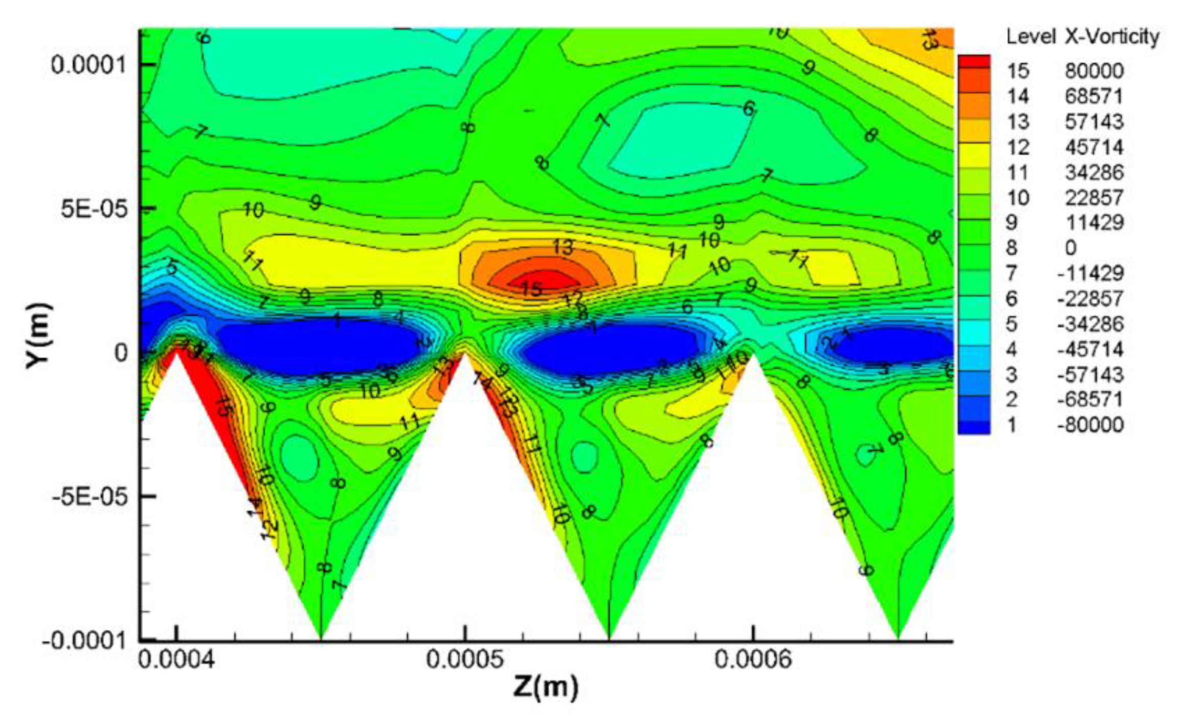
3.2.2. Triangular Groove Plate

The calculation conditions were the same as in the smooth plate model.

(1)

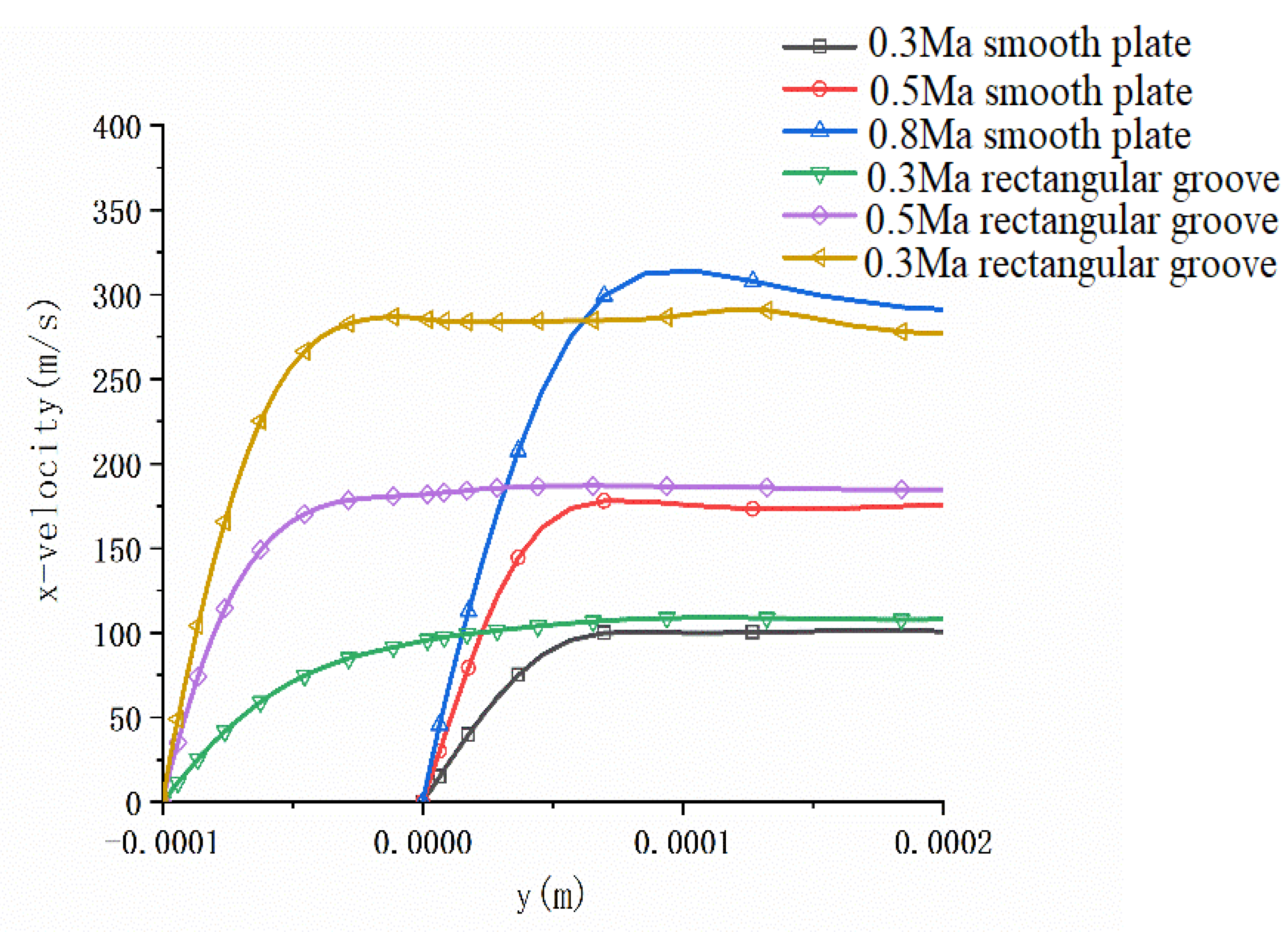
Velocity distribution

To facilitate the comparison of the influence of triangular grooves on the boundary layer velocity of the plate under subsonic flow, the flow velocity distribution of the smooth plate is presented in Figure 13. The data extraction plane is the vertical surface parallel to the flow direction located at the span z = 0.00055 m.

Figure 14 shows the velocity distribution of the triangular groove plate under subsonic flow. The data extraction plane is located in the vertical plane of the flow direction at z = 0.00055 m. The bottom of the plane reaches the bottom of the groove, which can reflect the flow field information inside the groove.

As the velocity increased, it could be found that the thickness of the boundary layer decreased gradually. When the velocity increased from 0.3 Ma to 0.5 Ma, the thickness of the boundary layer decreased by 0.00001 m at the flow direction x = 0.0037 m. When the velocity increased from 0.5 Ma to 0.8 Ma, the thickness of the boundary layer at the same position decreased by 0.00003 m. In other words, within the subsonic range, the boundary layer thickness decreased with the increase of velocity, and the faster the speed, the more the thickness of the boundary layer was reduced. By comparing the triangular groove plate and smooth plate, it can be clearly seen that the thickness of the bottom low-velocity fluid in the boundary layer of the groove plate was much larger than that of the smooth plate boundary layer, which means the velocity gradient on the wall of triangular grooves was relatively small.

As shown in Figure 15, it can be further observed that the velocity distribution curve on the normal vertical line at the flow direction was x = 0.00375 m and z = 0.00055 m. It can be seen that the thickness of the boundary layer of the triangular grooved plate was significantly larger than that of the smooth plate, and the boundary layer at the bottom of the triangle groove plate near-wall flow changed with height more gently than the smooth plate. This shows that in the boundary layer at the bottom of the triangle groove plate, the velocity gradient in the boundary layer was less than that of the smooth plate boundary layer.

Since the triangular grooves were longitudinally arranged in the spanwise direction and extended along the flow direction, there was a height difference of the wall in the span, and the velocity distribution could not be fully understood from the spanwise plane alone. Therefore, the spanwise plane at flow direction x = 0.00375 m was selected to make the velocity distribution cloud picture, as shown in Figure 16. As the velocity increased, the thickness of the boundary layer decreased in the spanwise direction; however, the variation of the thickness of the boundary layer in the spanwise direction was not the same at each point but fluctuated with the position. Under the above simulated velocity conditions, the boundary layer at the top of the groove was relatively the thinnest. At the bottom of the groove, the boundary layer thickness was the largest, and the change of boundary layer thickness with velocity was also the largest. At 0.8 Ma, the shape of the spanwise section of the boundary layer began to be close to that of the groove. It can be judged that as the velocity continued to increase, the boundary layer would further fit the groove, and the thickness difference of the boundary layer in the spanwise direction would decrease.

(2)

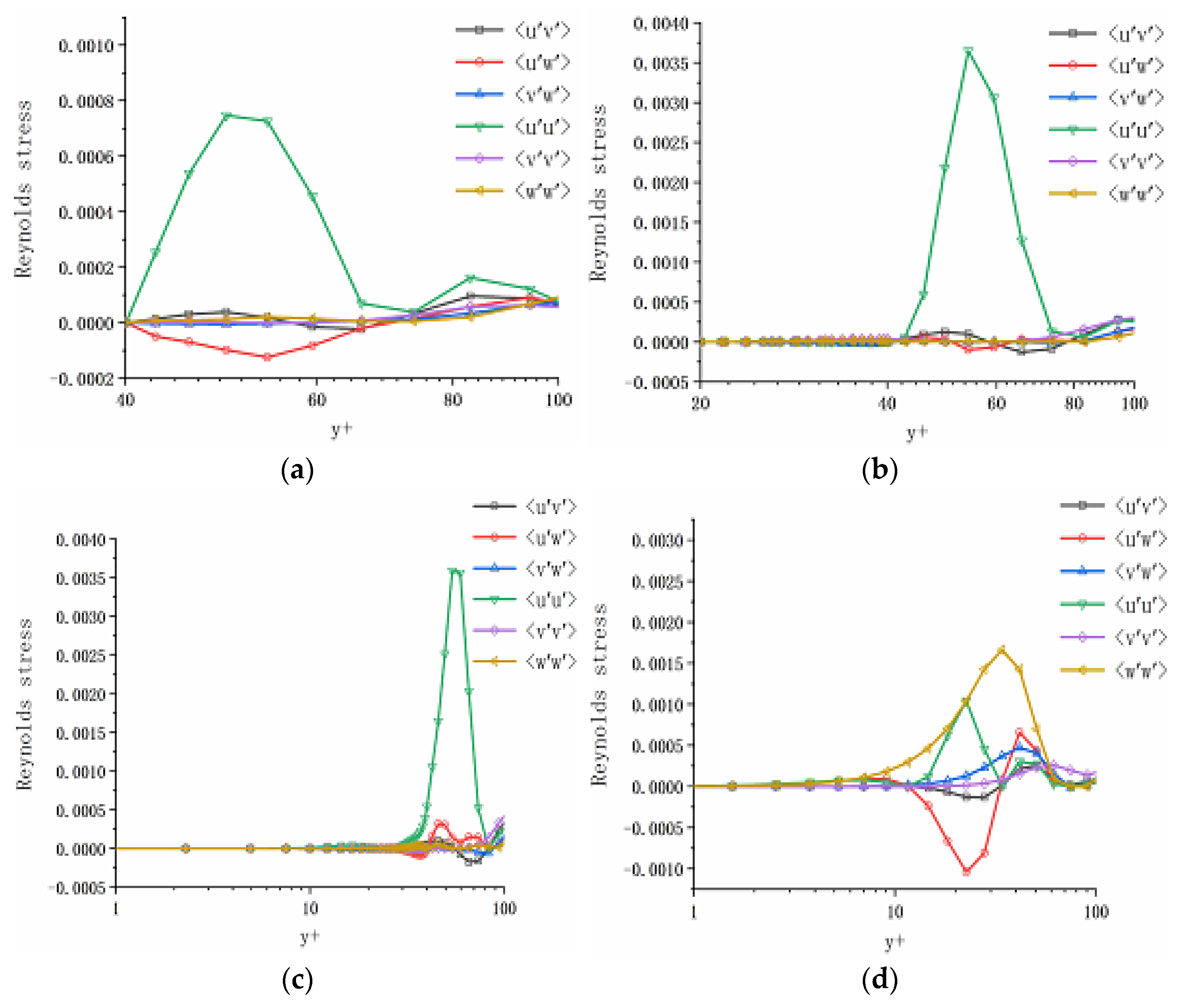
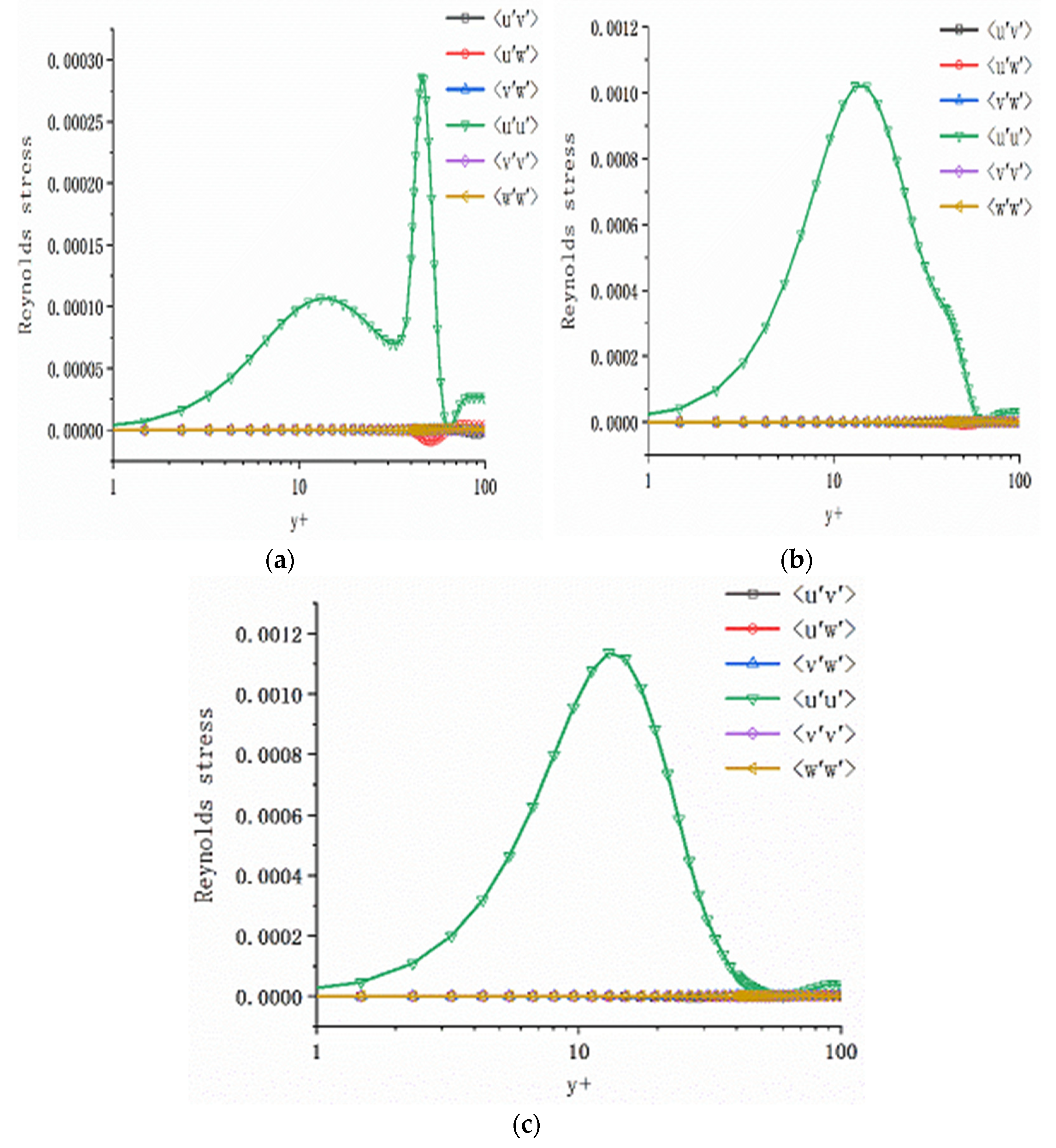
Reynolds stress

Reynolds stress is a special stress in turbulent motion, which is different from viscous stress and is an additional stress caused by the momentum exchange caused by turbulence pulsation. In the RANS equation, the Reynolds stress is expressed as $-\rho \overline{u_i^{\prime }{u}_j^{\prime }}$, where $\rho$ is the density of the fluid, the fluid is air, $u_i^{\prime }$ and $u_j^{\prime }$ is the pulsation value of the velocity component in each direction of the fluid, which can be expressed as $u^{\prime }$, $v^{\prime }$ and $w^{\prime }$, and $\overline{u_i^{\prime }{u}_j^{\prime }}$ represents the time mean of the product of the velocity pulsation. The dimensionless Reynolds stress is denoted by $\langle u_i^{\prime }{u}_j^{\prime }\rangle$ here and later.

For the convenience of comparison, data were extracted from the top, middle, and bottom of the groove wall, namely, the groove plate x = 0.00375 m, located on the three plumb lines with the span z = 0.0005 m, z = 0.000525 m, and z = 0.00055 m. For the smooth plate, a plumb line was selected at similar positions to extract the data. The distribution of Reynolds stress along the normal direction of the triangular groove plate and smooth plate is shown in Figure 17. For the triangular groove plate, the Reynolds normal stress component in the direction of flow $\langle u^{\prime }{u}^{\prime }\rangle$ is the largest among all the Reynolds normal stress components, and the maximum values of the Reynolds normal stress component in the middle and bottom of the groove are higher than those at the top of the groove. The reason for this situation is that the distance between the groove top wall and the maximum value $\langle u^{\prime }{u}^{\prime }\rangle$ is very small, and the wall has a strong blocking effect. Moreover, it is located at the bottom of the viscous layer, and the viscous force has a strong effect, which inhibits the velocity pulsation. The distance between the walls in the middle and bottom of the groove and the maximum value of $\langle u^{\prime }{u}^{\prime }\rangle$ is much larger than that at the top of the groove, because here it is the outer layer of the boundary layer, with turbulent development more fully, while at the same time, because the groove at the bottom of the central position and relative to the narrow stream flowing section, it has a strong disturbance to the coming flow. Therefore, the speed fluctuation is larger, caused here along the flow direction of the Reynolds normal stress component that is very large. By observing the Reynolds stress distribution of the smooth plate, it can be found that the maximum value of $\langle u^{\prime }{u}^{\prime }\rangle$ is equivalent to that of the top of the groove, but smaller than that of the middle and bottom of the groove, which indicates that the influence of the smooth plate on the incoming flow is the same as that of the top of the groove. In the Reynolds stress component of the smooth plate, the normal stress along the flow direction no longer plays a major role. It can be seen that the normal stress along the span $\langle w^{\prime }{w}^{\prime }\rangle$ is larger than the normal stress along the flow direction$\langle u^{\prime }{u}^{\prime }\rangle$, and the shear stress component along the span $\langle u^{\prime }{w}^{\prime }\rangle$ is equal in size $\langle u^{\prime }{u}^{\prime }\rangle$, while in the Reynolds stress component of the groove plate, the values of the normal stress $\langle w^{\prime }{w}^{\prime }\rangle$ and the shear stress along the span $\langle u^{\prime }{w}^{\prime }\rangle$ are very small. This means that grooves have an obstruction effect on the spreading flow in the boundary layer, which is consistent with the theory described in the second vortex group theory that states that grooves block disturbances between adjacent grooves and tends to influence the flows to be stable.

(3)

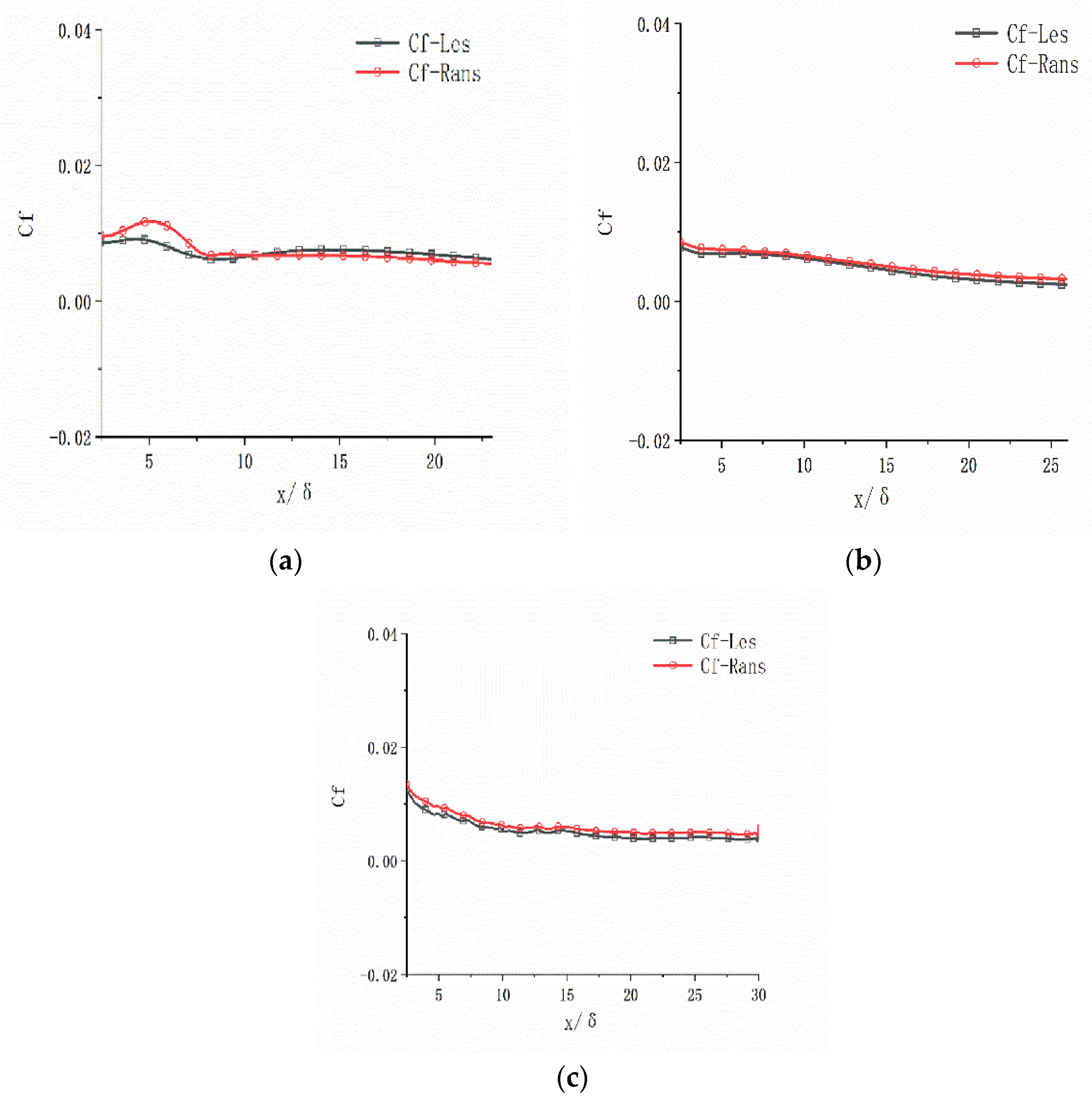
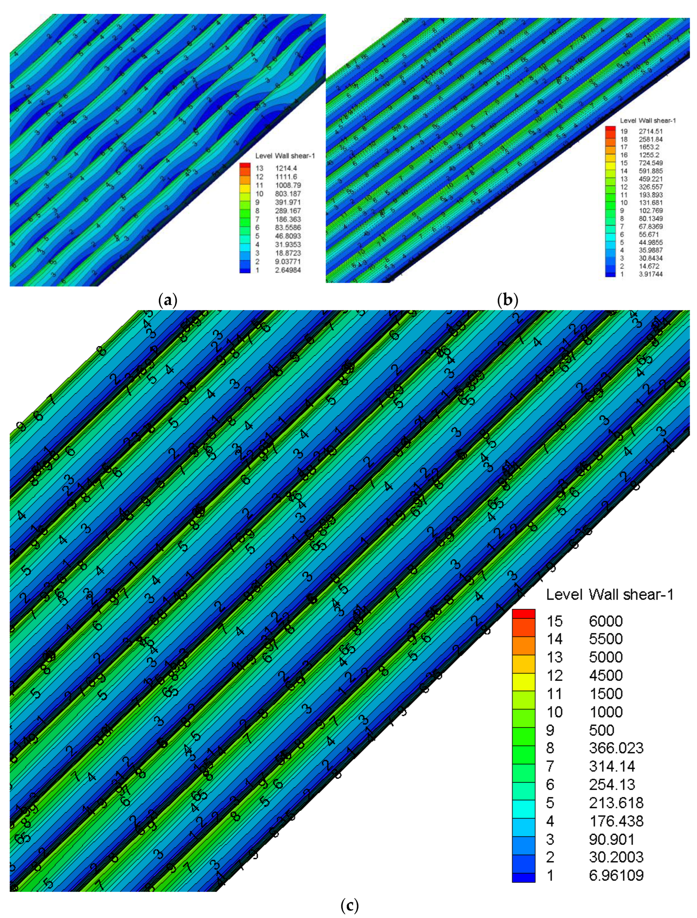
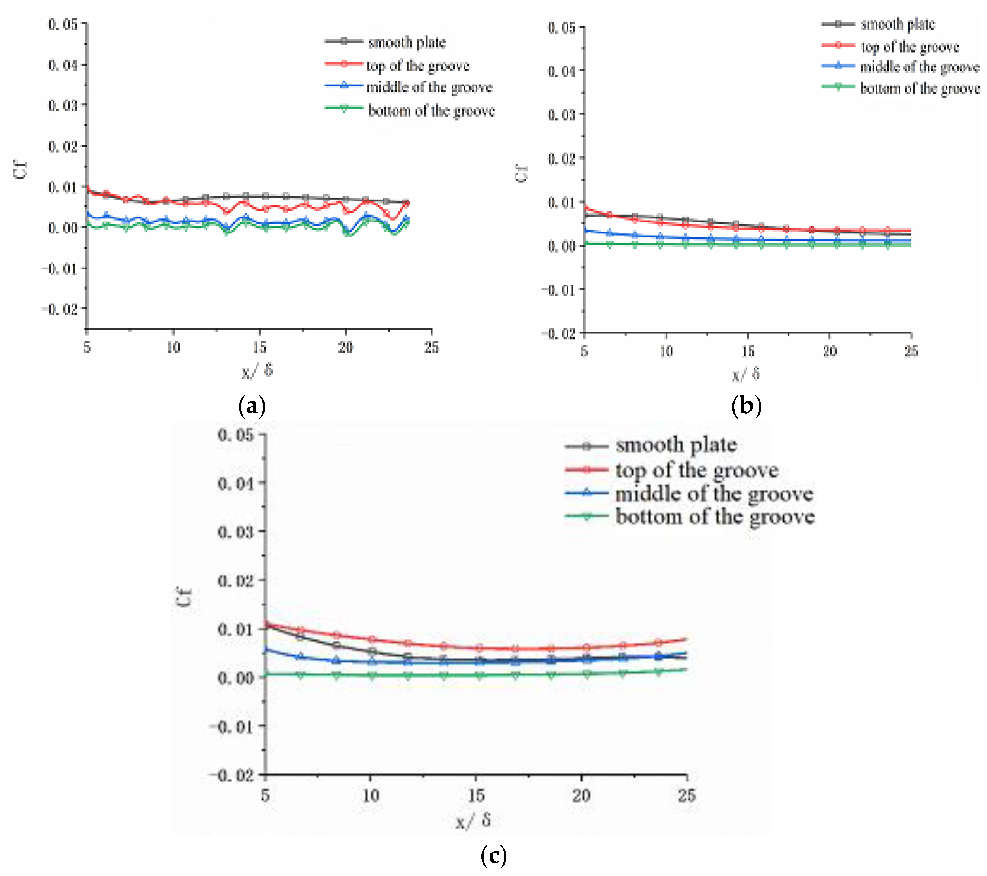
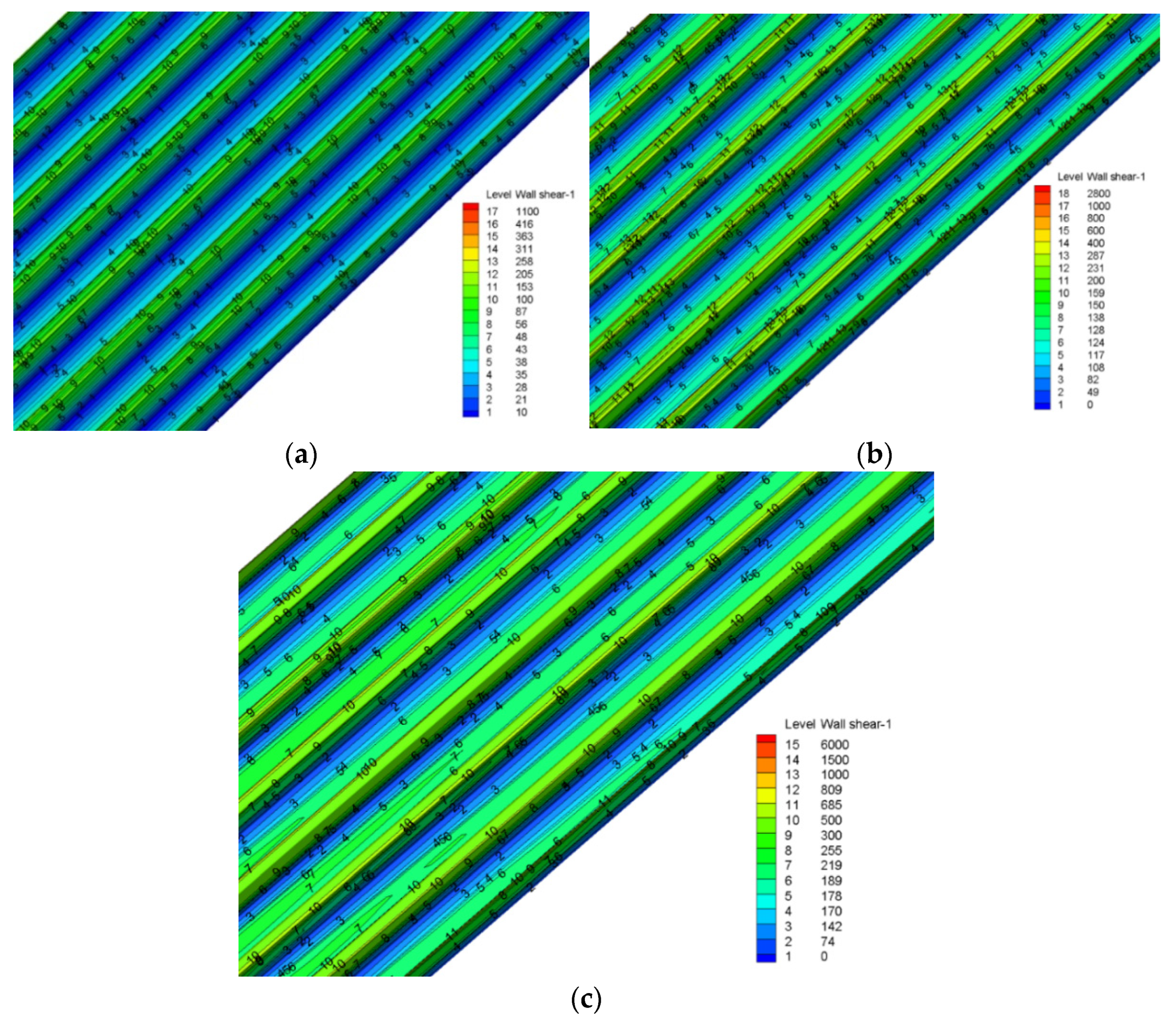
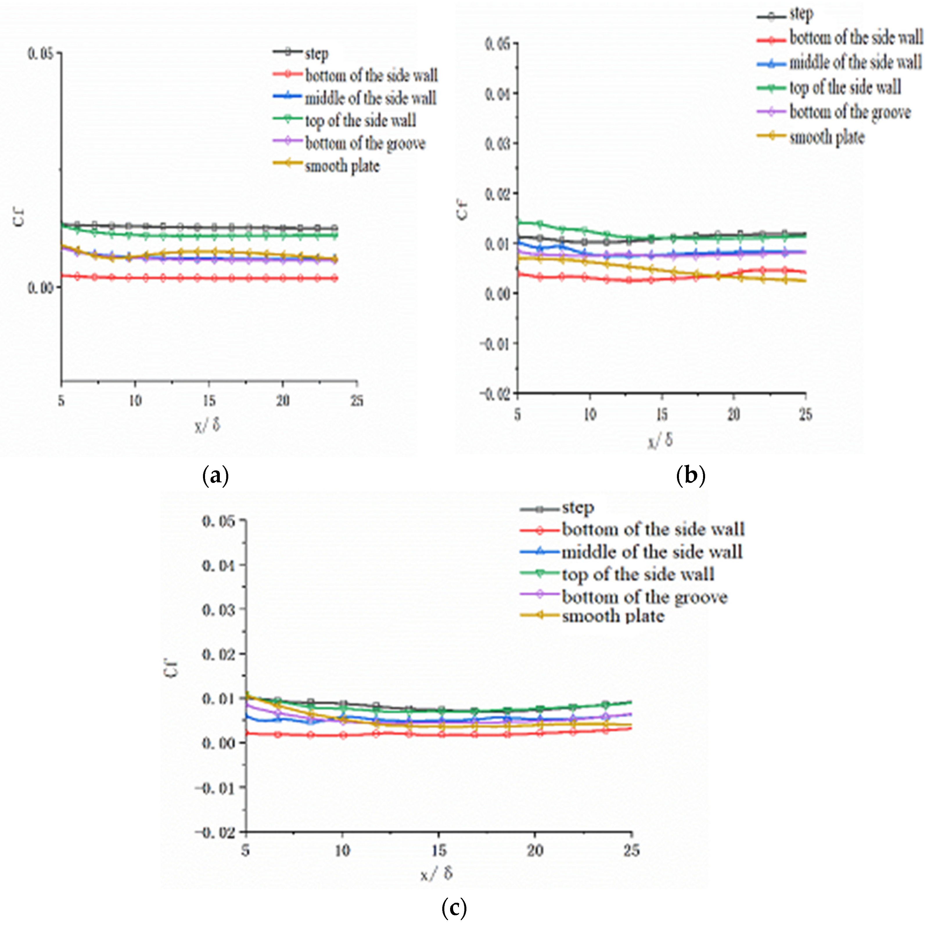
Wall shear stress

Figure 18 shows the wall shear stress distribution of the triangular groove plate. From the figure, we find with the increase in velocity, that the wall shear stress increases. The wall shear stress is periodically distributed along the spanwise of the triangular groove plate, which corresponds to the periodic arrangement of grooves along the spanwise. In the triangular groove, the shear stress on the wall surface is not uniformly distributed, but gradually decreases from the top to the bottom of the groove, while the shear stress tends to be uniformly distributed in the flow direction.

To further analyze the wall shear stress, the straight lines along the flow direction were taken at the top, middle and bottom of the wall of the triangular groove, respectively. The specific position was at the flow direction x = 0.00375 m, and the span z = 0.00050625 m, z = 0.000525 m, and z = 0.00054375 m, respectively, and the data on the straight lines were extracted. The shear stress coefficient distribution curve is shown in Figure 19.

As can be seen from the figure, at 0.3 Ma and 0.5 Ma, the wall shear stress coefficient at the top of the groove was the largest, which was close to that of the smooth plate, and the shear stress coefficient at the middle and bottom of the wall was significantly smaller than that at the top of the groove. When the velocity increased to 0.8 Ma, the shear stress coefficient at the top of the groove exceeded that of the smooth plate, and the shear stress coefficient in the middle of the groove was similar to that of the smooth plate. This shows that with the increase in incoming flow velocity, the effect of the triangular groove plate on shear stress reduction became weaker. Combined with Figure 19a–c, the thickness of the boundary layer from the top of the groove to the bottom of the groove was increased due to the presence of a hypotenuse in the triangle. As the height of the inclined wall changed, the average velocity gradient at the wall also changed spanwise. When the average velocity gradient decreased gradually from the top to the bottom of the groove, the shear stress at the wall increased gradually from the bottom to the top of the groove. When the flow velocity increased, the shear stress increased more with the groove wall near the top.

Figure 20 is the flow velocity cloud picture of triangular grooves on the λ isosurface, which reflects the three-dimensional structure of vorticity. Figure 21 is the flow vorticity distribution cloud picture, which is on the span plane. Combined with Figure 20 and Figure 21, the streamwise vortices mainly existed above the top of the groove, and as can be seen from Figure 21, there were vortices with opposite rotation directions above the groove. From the three-dimensional structure of the vortex as shown in Figure 20, the vortices in the boundary layer tended to rise upwards, this was because the flow direction vortex pulled the low-velocity fluid at the bottom of the boundary layer and carried it away from the wall. Due to the departure of the bottom fluid, the upper fluid of the boundary layer will flow downward and pour into the bottom, and the relative flow between the different flow layers will lead to the mixing of the various flow layers in the boundary layer, causing the exchange of momentum, energy and mass with additional drag. At the top of the groove wall, there are secondary vortices induced by the streamwise vortices above the groove. According to the theory of the second vortex group, these secondary vortices can suppress the rise of the low speed strip in the groove and reduce the burst of turbulence.

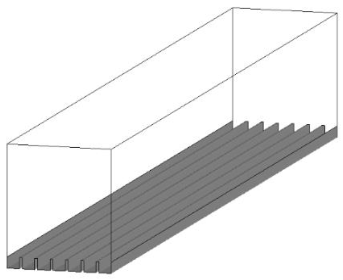
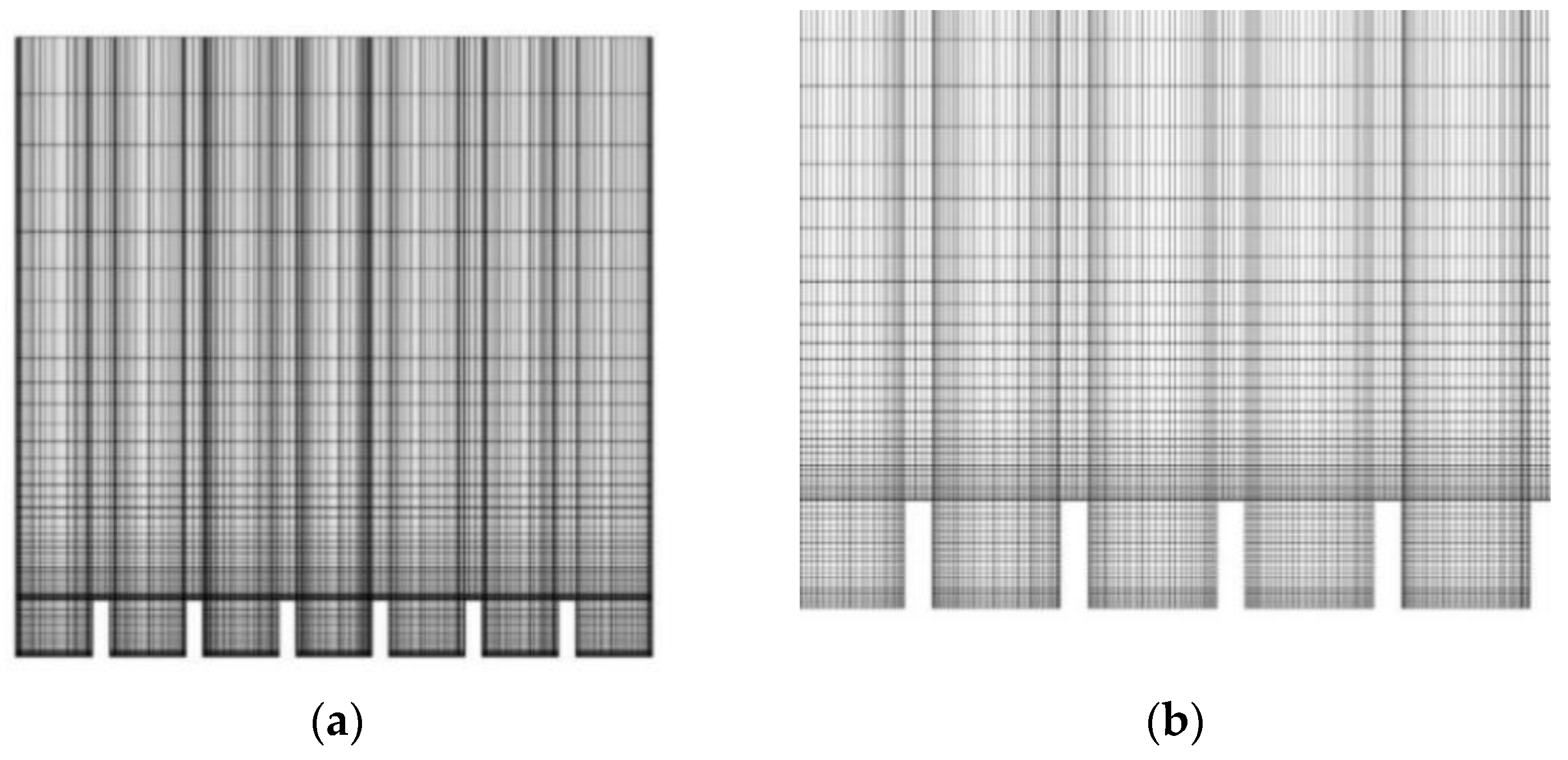
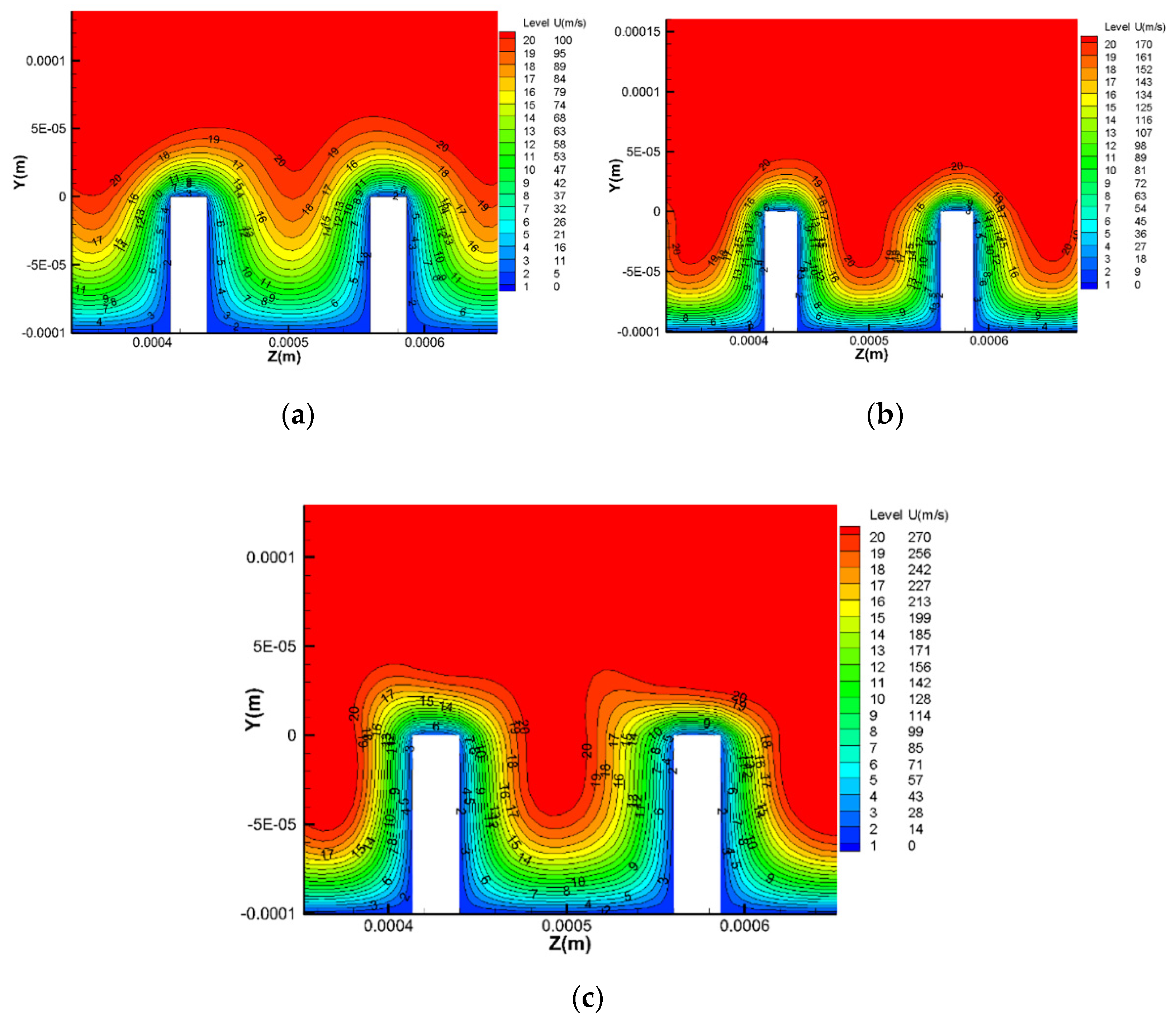
3.2.3. Rectangular Groove Plate

The calculation conditions are the same as in the smooth plate model.

(1)

Velocity distribution

Figure 22 shows the velocity cloud pictures of the rectangular groove plate with incoming velocities of 0.3 Ma, 0.5 Ma and 0.8 Ma, respectively. The data extraction plane is located at the plumb surface of the flow direction at z = 0.0005 m.

There was a great difference between the boundary layer of the rectangular groove plate and that of the triangular groove plate. On one hand, at the same speed, the boundary layer thickness of the rectangular groove plate was smaller than that of the triangular groove plate. On the other hand, there was a thick low-velocity layer at the bottom of the boundary layer of the triangular grooved plate, while the low-velocity layer at the bottom of the boundary layer of the rectangular grooved plate was very thin. With the increase in incoming flow velocity, the change of boundary layer thickness of rectangular groove plate became smaller.

Figure 23 shows the velocity profile of the rectangular groove and smooth plate at the normal perpendicular at the flow direction x = 0.00375 m and span z = 0.0005 m. The velocity profile of the rectangular groove was the same as that of the smooth plate. The boundary layer thickness of the rectangular groove was the same as that of the smooth plate, and the velocity gradient at the bottom of the boundary layer was the same as that of the smooth plate.

Considering the rectangular grooves are longitudinally arranged in the spanwise direction and extending along the flow direction, there was a height change of the wall surface in the span. The spanwise plane located at the flow direction x = 0.00375 m was taken to make the velocity distribution cloud picture, as shown in Figure 24.

As can be seen from the figure, compared with the triangular groove, the boundary layer of the rectangular groove began to fit the groove at 0.3 Ma, and this phenomenon became more obvious with the increase in the Mach number. Observing the bottom of the rectangular groove, there was a relatively thick low-velocity bottom layer at the intersection of the plumb wall and the bottom wall of the groove. This was because the flow at this point was affected by the spanwise wall and the normal wall at the same time, the blocking effect was strong, and the low-velocity fluid was retained here.

(2)

Reynolds stress

For the analysis of Reynolds stress in the boundary layer of the rectangular groove, three normal straight lines from near to far from the plumb wall were selected, which were located at x = 0.00375 m, z = 0.00044625 m, z = 0.00047 m and z = 0.0005 m, respectively. A flow speed of 0.3 Ma was taken for analysis, as shown in Figure 25.

As can be seen from the figure, normal stress along the flow direction $\langle u^{\prime }{u}^{\prime }\rangle$ played a major role in the boundary layer of the rectangular groove, but compared with the Reynolds stress inside the triangular groove, it can be found that the value of Reynolds stress inside the rectangular groove was very small. By comparing Figure 25a–c, it can be found that the Reynolds stress component $\langle u^{\prime }{u}^{\prime }\rangle$ near the plumb wall was smaller than that farther away from the plumb wall at the same height. This indicates that at 0.3 Ma, the rectangular groove plumb wall had a strong blocking effect on the incoming flow, and a strong restraining effect on the upward turbulence pulsation of convective flow, which reduced the Reynolds stress component $\langle u^{\prime }{u}^{\prime }\rangle$ in the boundary layer. In Figure 25a, the maximum value of the Reynolds stress component $\langle u^{\prime }{u}^{\prime }\rangle$ near the plumb wall appeared later than that in Figure 25b,c, indicating that the plumb wall not only reduced the Reynolds stress but also delayed the position of the Reynolds stress peak.

(3)

Wall shear stress

The wall shear stress distribution of the rectangular groove plate is shown in Figure 26. The overall distribution of the wall shear stress was similar to that of the triangular groove plate, which presented a periodic distribution along the span, and the shear stress increased with the increase in velocity. Inside the rectangular groove, the shear stress on the plumb wall increased gradually from the bottom of the wall to the top, and the shear stress was evenly distributed in the direction of flow.

For further analysis of the wall shear stress of the rectangular groove, five straight lines along the flow direction were taken on the wall. The specific positions of the straight lines were, respectively, in the top step of groove y = 0 m, z = 0.0004271 m, the top, middle and bottom parts of groove plumb wall z = 0.00044 m corresponding to y = −0.00001 m, y = −0.00005 m, y = −0.00009 m and y = −0.0001 m, z = 0.0005 m at the bottom of the groove. The data extracted on a straight line with the drawn shear stress distribution curve are shown in Figure 27.

As can be seen from Figure 27, the maximum wall shear stress of the rectangular groove plate was at the step at the top of the groove, which was higher than that on the smooth plate. The minimum shear stress coefficient of the rectangular groove was located at the bottom of the plumb wall, which was less than that of the smooth plate, while at the bottom of the rectangular groove, the magnitude of the shear stress coefficient was basically the same as that of the smooth plate.

From Figure 27a–c, we can see that the groove at the top of the step in the boundary layer thickness was small and the low speed at the bottom of the thickness was less than the other in the same position. Compared with the boundary layer of the smooth plate, the thickness of the boundary layer and the thickness of the low-velocity bottom layer at the top step of the rectangular groove were smaller than those of the smooth plate, therefore, the shear stress there was larger than that of the smooth plate. Along the plumb wall from top to bottom, the thickness of the low-speed bottom layer on the plumb wall was gradually increased. At the bottom of the groove, the thickness of the low-velocity bottom decreased gradually along the spanwise direction and reached the minimum at the middle of the bottom of the rectangular groove, where the thickness of the low-velocity bottom was equivalent to that of the smooth plate. According to the thickness variation rule of the low-speed bottom layer in the rectangular groove, it can be concluded that the shear stress of the wall at more than half the height of the groove inside the rectangular groove was greater than that of the smooth plate, and that the shear stress of the wall below half the height of the groove was smaller than that of the smooth plate.

The frictional resistance coefficients of the smooth plate, triangular groove plate and rectangular groove plate under subsonic flow are shown in

Table 3. Frictional drag coefficient of plates with different surfaces at different speeds.

Ma	Smooth Plate	Triangular Groove	Rectangular Groove
0.3	0.007312	0.006767	0.008555
0.5	0.005959	0.005472	0.009364
0.8	0.007727	0.006891	0.007451

. It can be seen from the table that compared with the smooth plate, the friction resistance coefficient of the triangular groove plate was lower than that of the smooth plate at all speeds, showing the drag reduction characteristics. At 0.3 Ma and 0.5 Ma, the frictional drag coefficient of the rectangular groove plate was higher than that of the smooth plate. At this time, the rectangular groove plate showed a drag increase; however, with the speed reaching 0.8 Ma, the frictional drag coefficient of the rectangular groove plate was lower than that of the smooth plate, showing a drag reduction characteristic.

Figure 28 shows the flow velocity cloud picture of the rectangular groove on the λ isosurface, and the three-dimensional structure of vortices on the rectangular groove. Figure 29 shows the stream-direction vortex of the flow field in the rectangular groove. The data extraction plane was the plumb plane perpendicular to the stream-direction x = 0.00375 m. From Figure 28 and Figure 29, the flow of the rectangle grooves’ flat vortex and triangular groove plate flow vortex distribution can be seen, where a flow to the vortex mainly existed in the top of the groove, and the vortex also showed a trend of rising but was different from the triangular groove. The vortex movement in the span was weaker than that of the triangular groove and this means that the spanwise pulsation of the rectangular groove was smaller. At the wall of the rectangular groove, only the wall on the top step had a secondary vortex, which had a weak influence on the spanwise wall, leading to a weak suppression of burst in the groove.

4. Conclusions

According to the current research, the frictional resistance of fluid flowing through the groove surface is smaller than that of fluid flowing through the smooth plate. To explore the influence of different surface structures on the flow inside the boundary layer at different speeds, the large eddy simulation (LES) method was adopted in this paper. Based on the computational fluid dynamics software, Fluent, the plate with a triangular groove and rectangular groove under subsonic flow were simulated, respectively. Then, the boundary layer was analyzed from the velocity distribution, Reynolds stress, wall shear stress, and streamwise vortex, and the following conclusions were drawn.

(1)

The triangular groove structure along the flow direction can reduce frictional resistance under subsonic flow, but the drag reduction effect will decrease with the increase in velocity. The rectangular groove structure has different effects on the friction resistance at different speeds. The friction increases when the speed is below 0.8 Ma and decreases when the speed is above 0.8 Ma.

(2)

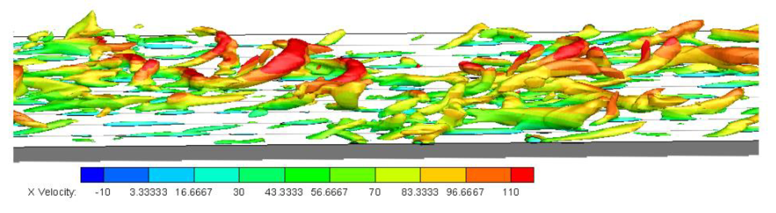
By analyzing the velocity distribution, Reynolds stress, and flow vortices of triangular grooves, it was found that triangular grooves increase the blocking effect of the wall on the fluid, which is equivalent to increasing the thickness of the viscous bottom layer, and reduces the velocity gradient near the wall, thus reducing the wall shear stress. The variation of the height of the groove structure spanwise will affect the thickness of the boundary layer, resulting in a variation of the shear stress on the wall spanwise, and also reducing the spanwise component of the Reynolds stress, indicating that the groove structure weakens the burst on the wall. In addition, the groove structure also obstructs the spanwise flow and inhibits the occurrence of spanwise disturbance.

(3)

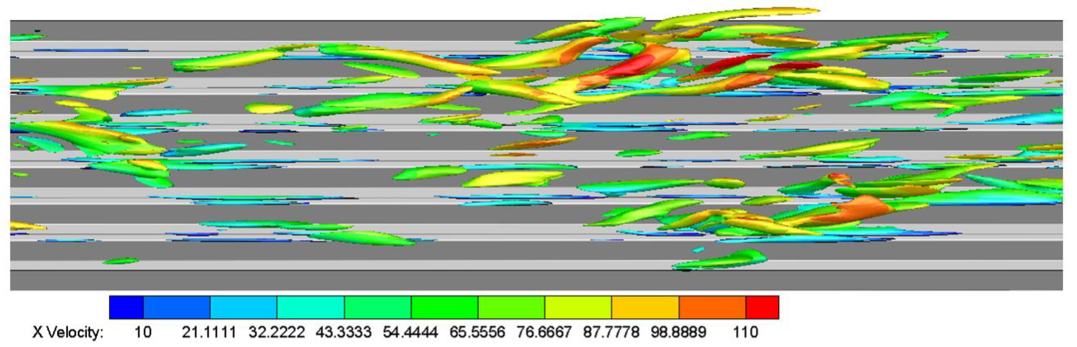
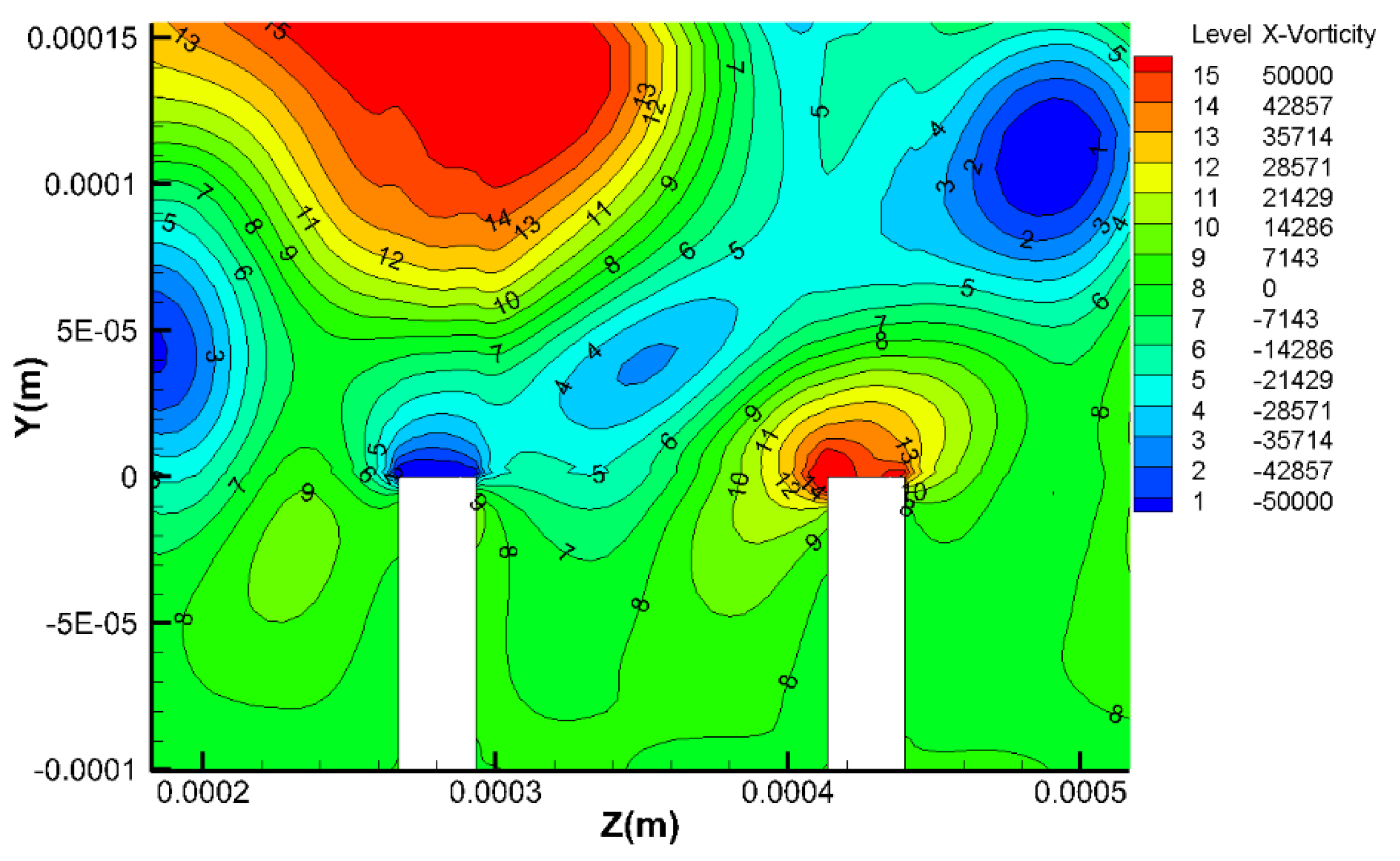
The drag reduction effect of the rectangular groove structure will appear only when the velocity is large enough that the flow vortex moves down into the groove.

According to the flow vorticity analysis, the secondary vortices in the rectangular groove can suppress the burst of turbulence, thereby reducing the wall shear stress. Therefore, the drag reduction effect of the triangular groove is better than that of the rectangular groove under subsonic conditions.

References

- Schrauf, G.; Wood, N.; Gölling, B. Key aerodynamic technologies for aircraft performance improvement. In Proceedings of the 5th Community Aeronautics Days, Vienna, Austria, 19–21 June 2006. [Google Scholar]
- Liepmann, H.W. The rise and fall of ideas in turbulence. Am. Sci. 1979, 67, 221–228. [Google Scholar]
- Perlin, M.; Dowling, D.R.; Ceccio, S.L. Freeman scholar review: Passive and active skin friction drag reduction in turbulent boundary layers. J. Fluids Eng. 2016, 138, 91–104. [Google Scholar] [CrossRef]
- Tiong, A.N.T.; Kumar, P.; Saptor, A. Reviews on drag reducing polymers. Korean J. Chem. Eng. 2015, 32, 1455–1476. [Google Scholar] [CrossRef]
- Bechert, D.W.; Hoppe, G.; Reif, W.E. On the drag reduction of the shark skin. In Proceedings of the 23rd Aerospace Sciences Meeting, Reno, NV, USA, 14–17 January 1985. [Google Scholar] [CrossRef]
- Szodruch, J. Viscous drag reduction on transport aircraft. In Proceedings of the 29th Aerospace Sciences Meeting, Reno, NV, USA, 7–10 January 1991. [Google Scholar] [CrossRef]
- Brian, D.; Bharat, B.; Yang, S.; Li, S.; Tian, H.; Li, Y. Research Progress on Drag Reduction of Sharkskin Surface Fluid in Turbulent Flow. Adv. Mech. 2012, 42, 821–836. [Google Scholar] [CrossRef]
- Walsh, M.J. Turbulence Boundary Layer Drag Reduction Using riblets. In Proceedings of the AIAA 20th Aerospace Sciences Meeting, Orlando, FL, USA, 11–14 January 1982; AIAA-82. pp. 1–9. [Google Scholar] [CrossRef]
- Walsh, M.J. Riblets as a viscous drag reduction technique. AIAA J. 1983, 21, 485–486. [Google Scholar] [CrossRef]
- Walsh, M.J.; Lindemann, A.M. Optimization and Application of Riblets for Turbulent Drag Reduction. In Proceedings of the AIAA 22nd Aerospace Sciences Meeting, Reno, NV, USA, 9–12 January 1984. AIAA-84. [Google Scholar] [CrossRef]
- Hefner, J.N.; Bushnell, D.M.; Walsh, M.J. Research on non-planar wall geometries for turbulence control and skin-friction reduction. In Proceedings of the 8th U. S. -FRG DEA Meeting, Viscous and Interacting Flow Field Effects, Gottingen, Germany, 1983. [Google Scholar]
- Bacher, E.V.; Smith, C.R. A combined visualization-anemometry study of the turbulent drag reducing mechanisms of triangular micro-groove surface modifications. In Proceedings of the Shear Flow Control Conference, Boulder, CO, USA, 12–14 March 1985. [Google Scholar] [CrossRef]
- Gallagher, J.A.; Thomas, A.S.W. Turbulent boundary layer characteristics over streamwise grooves. In Proceedings of the 2nd Applied Aerodynamics Conference, Seattle, WA, USA, 21–23 August 1984. AIAA-84-2185. [Google Scholar] [CrossRef]
- Bechert, D.W.; Bruse, M.; Hage, W. Experiments with three-dimensional riblets as an idealized model of shark skin. Exp. Fluids 2000, 28, 403–412. [Google Scholar] [CrossRef]
- Park, S.R.; Wallace, J.M. Flow alteration and drag reduction by riblets in a turbulent boundary layer. AIAA J. 1994, 32, 31–38. [Google Scholar] [CrossRef]
- Gaudet, L. Properties of riblets at supersonic speed. Appl. Sci. Res. 1989, 46, 245–254. [Google Scholar] [CrossRef]
- Coustols, E.; Cousteix, J. Experimental Investigation of Turbulent Boundary Layers Manipulated with Internal Devices: Riblets. In Structure of Turbulence and Drag Reduction. International Union of Theoretical and Applied Mechanics; Gyr, A., Ed.; Springer: Berlin/Heidelberg, Germany, 1990. [Google Scholar] [CrossRef]
- Sundaram, S.; Viswanath, P.R.; Rudrakumar, S. Viscous drag reduction using riblets on NACA 0012 airfoil to moderate incidence. AIAA J. 1996, 34, 676–682. [Google Scholar] [CrossRef]
- Subashchandar, N.; Rajeev, K.; Sundaram, S. Drag Reduction Due to Riblets on NACA0012 Airfoil at Higher Angles of Attack. In National Aerospace Laboratories; Rept. PD EA 9504; National Aerospace Laboratories: Bangalore, India, 1995. [Google Scholar]
- Launder, B.E.; Li, S.P. On the Prediction of Riblet Performance with Engineering Turbulence Models. Appl. Sci. Res. 1993, 50, 283–298. [Google Scholar] [CrossRef]
- Caram, J.M.; Ahmed, A. Effect of riblets on turbulence in the wake of an airfoil. AIAA J. 1991, 29, 1769–1770. [Google Scholar] [CrossRef]
- McLean, J.D.; George-Falvy, D.N.; Sullivan, P.P. Flight-test of turbulent skin-friction reduction by riblets. In International Conference on Turbulent Drag Reduction by Passive Means; OpenSky: London, UK, 1987; pp. 408–428. [Google Scholar]
- Debisschop, J.R.; Nieuwstadt, F.T.M. Turbulent boundary layer in an adverse pressure gradient—Effectiveness of riblets. AIAA J. 1996, 34, 932–937. [Google Scholar] [CrossRef]
- Djenidi, L.; Antonia, R.A. Laser Doppler anemometer measurements of turbulent boundary layer over a riblet surface. AIAA J. 1996, 34, 1007–1012. [Google Scholar] [CrossRef]
- Dean, B.; Bhushan, B. Shark-skin surfaces for fluid-drag reduction in turbulent flow: A review. Philos. Trans. R. Soc. A Math. Phys. Eng. Sci. 2012, 42, 821–836. [Google Scholar] [CrossRef]
- Chu, D.C.; Karniadakis, G.E. A direct numerical simulation of laminar and turbulent flow over riblet-mounted surfaces. J. Fluid. Mech. 1993, 250, 1–42. [Google Scholar] [CrossRef] [Green Version]
- Peet, Y.; Sagaut, P.; Charron, Y. Turbulent drag reduction using sinusoidal riblets with triangular cross-section. In Proceedings of the 38th AIAA Fluid Dynamics Conference and Exhibit, Seattle, WA, USA, 23–26 June 2008; AIAA: Seattle, WA, USA, 2008; pp. 1–9. [Google Scholar] [CrossRef] [Green Version]
- Fu, H.; Shi, X.; Qiao, Z. Numerical analysis of drag Reduction characteristics of fringe films. J. Northwestern Polytech. Univ. 1999, 11, 25–30. [Google Scholar]
- Du, J.; Gong, M.; Tian, A.; Gao, N.; Li, Z. Research on Drag Reduction of High-speed Train Based on Bionic Non-Smooth Groove. J. Railw. Sci. Eng. 2014, 11, 70–76. [Google Scholar] [CrossRef]
- Wang, J.; Chen, G. Experimental Study on Quasi-ordered Structures in The Near Wall Region of Turbulent Boundary Layer on Groove Surface. J. Aviat. 2001, 022, 400–405. [Google Scholar] [CrossRef]
- Feng, Y.; Cong, Q.; Jin, J.; Zhang, H.; Ren, L. Numerical Analysis of Flow Field on Non-smooth Surface of Groove. J. Jilin Univ. (Eng. Sci.) 2006, 36, 103–107. [Google Scholar] [CrossRef]
- Cong, Q.; Feng, Y. Numerical Simulation of Flow Field on Triangular Groove Surface. Ship Mech. 2006, 10, 11–16. [Google Scholar] [CrossRef]
- Huang, W.; Wang, B.; Lu, M.; Chen, G.; Zhang, X. Numerical Simulation of Geometrical Shape of Trailing Wave Biomimetic Drag Reduction Material. Ship Mech. 2005, 9, 14–17. [Google Scholar] [CrossRef]
- Li, Y.; Qiao, Z.; Wang, Z. Experimental Study on Drag Reduction of Furrow Film on Outer Surface of Yun-7 Aircraft. Pneum. Exp. Meas. Control. 1995, 21–26. [Google Scholar]
- Hu, H.; Song, B.; Mao, Z.; Chen, S. Research on Drag and Noise Reduction Mechanism of Traveling Wave Surface. Fire Control. Command. Control. 2007, 32, 28–30. [Google Scholar] [CrossRef]
- Hu, H.; Song, B.; Pan, G.; Mao, Z.; Chen, S. Experimental Study on Drag Reduction of Water Tunnel with Stripe Grooves on Rotary Surface. Q. Mech. 2006, 27, 267–272. [Google Scholar] [CrossRef]
- Zhang, B. Experimental Study on Drag Reduction Mechanism of Turbulent Boundary Layer on Groove Wall. Master’s Thesis, Tianjin University, Tianjin, China, 2007. [Google Scholar]
- Chang, Y. Experimental Study on Drag Reduction Mechanism of Groove Wall in Turbulent Boundary Layer. Ph.D. Thesis, Tianjin University, Tianjin, China, 2009. [Google Scholar]
- Huang, Z. Basic Research on Shark Skin Microgroove Replication Technology Based on Structural Bionics. Master’s Thesis, Dalian University of Technology, Dalian, China, 2012. [Google Scholar]
- Sun, P. Basic Research on Drag Reduction Mechanism and Replication Technology of Shark Skin Microgrooves. Master’s Thesis, Dalian University of Technology, Dalian, China, 2010. [Google Scholar]
- Li, X.; Dong, S.; Zhao, Z. Experimental Study on Drag Reduction effect of Small Scale Trench Surface. Min. Mach. 2006, 34, 91–93. [Google Scholar]
- Liu, Z.; Hu, H.; Song, B. Numerical Simulation of Drag Reduction on Ridged Surfaces with Different Intervals. J. Syst. Simul. 2009, 21, 6025–6028. [Google Scholar]
- Roidl, B.; Meinke, M.; Schröder, W. A reformulated synthetic turbulence generation method for a zonal RANS–LES method and its application to zero-pressure gradient boundary layers. Int. J. Heat Fluid Flow 2013, 44, 28–40. [Google Scholar] [CrossRef]