Long-Term Orbit Prediction and Deorbit Disposal Investigation of MEO Navigation Satellites

Abstract

With the increase in satellites in the medium Earth orbit (MEO) region, there should be a focus on orbit safety in the MEO region. A safe orbit disposal strategy is necessary to maintain the sustainability of the MEO region. This paper focuses on long-term evolution modeling, safety analysis of MEO objects, and different disposal techniques for end-of-life BDS-2 MEO satellites. On the one hand, a long-term numerical evolution model is established, and mean equinoctial elements are adopted to propagate a long-term orbit. Long-term evolution for the MEO region over 100 years is carried out, including the Galileo, BDS, GPS, and GLONASS constellations. The earliest orbit intersection time with other global navigation satellite system (GNSS) constellations is put forward. On the other hand, a dynamic model and an optimization model for disposal orbit are established, which minimize the eccentricity growth within 200 years and the fuel consumption for maneuvering to the disposal orbit. The bounds for the disposal region of BDS MEO satellites are also proposed, which consider the measurement and control error of BDS MEO satellites and the eccentricity bounds for end-of-life BDS MEO satellites. A genetic algorithm is adopted to optimize the orbital elements for end-of-life BDS MEO satellites. In addition, two disposal cases, namely, upraising and reducing the orbit, for end-of-life BDS MEO satellites are simulated. The long-term evolutions for the disposal of orbital elements within 200 years are implemented, and the fuel consumption is calculated. The results show that the current MEO region is relatively safe and that the eccentricity is the most important factor that influences the long-term evolution of safety analysis for BDS MEO disposal orbits. Upraising the orbit is safe for end-of-life BDS MEO satellites. This investigation provides the theoretical foundation for investigating the long-term evolutionary mechanisms of the MEO region and references disposal strategy analysis for decommissioned navigation satellites, and the spent upper stages for other GNSS constellations.

1. Introduction

Medium Earth orbit (MEO) is mainly used for satellite navigation nowadays. With the modernization of GPS and GLONASS and the construction of BDS and Galileo, an increasing number of satellites are launched into the MEO region. In the meantime, decommissioned navigation satellites and spent upper stages are left in the MEO region. The MEO region will be considerably congested. For the orbit of space debris, including decommissioned navigation satellites and spent upper stages in the MEO region, changes over hundreds of years under perturbation forces may lead to many orbit intersections with the global navigation satellite system (GNSS) orbit region. This may raise the collision probability of the MEO region.

Based on up-to-date data(as of 1 May 2022) [1], 32 GPS satellites are in orbit, including seven GPS II-R satellites, eight GPS IIR-M satellites, 12 GPS II-F satellites, and five GPS III-A satellites, of which 28 satellites are healthy. Twenty-five GLONASS satellites are in orbit, including 23 satellites that are operational and two satellites that are flight testing. Forty-nine BDS satellites are in orbit, of which 44 satellites are in operation. Twenty-six Galileo satellites are in orbit. The nominal orbital altitudes of GPS, GLONASS, BDS, and Galileo are approximately 20,196, 19,129, 21,528, and 23,200 km, respectively.

Three approaches, namely, numerical, analytical, and semi-analytical methods [2], are usually adopted to propagate a satellite orbit. Once the initial orbital elements are given, numerical methods, such as the Euler integral, Runge–Kutta integral, and Adams–Cowell method, can be used to update the orbital elements. For analytical methods, quasi mean orbital elements or mean orbital elements can be used. The quasi mean orbital element method excludes the short periodical term, and the mean orbital elements exclude the long and short periodical terms [3]. The key to semi-analytical methods is to obtain the average perturbation acceleration [4,5]. Two methods can be used: one is analytical averaging, and the other is numerical averaging. As to the analytical averaging method, two formats can be used: one is a non-Hamiltonian format, and the other is a Hamiltonian format [6,7].

BDS, GLONASS, Galileo, and two GPS satellites are equipped with Satellite Laser Ranging (SLR) retroreflectors. ESA uses laser ranging, passive optical methods, and radar to determine the spin parameters of inactive satellites [8]. Kucharski et al. investigated the influence of solar radiation pressure on satellite rotation through satellite laser ranging measurements, and the prediction accuracy will be improved if realistic surface force modeling is incorporated into orbit propagation algorithms [9].

The MEO region is not only the area where navigation satellites are located but is also an area where considerable carrier rocket debris and upper stage stagnation occur. Owing to the low space density and collision risk, it is currently a nonprotected area in space. The Inter-Agency Space Debris Coordination Committee provided guidelines for the disposal of spacecraft in the GEO and LEO regions [10]. Nevertheless, the guideline for the deorbit of spacecraft in the MEO region is currently unclear. The orbit life of decommissioned spacecraft and spent upper stages should be reduced through orbital maneuvers. The International Organization for Standardization and the European Cooperation for Space Standardization proposed that a disposal orbit should not intersect with the GEO region for at least 100 years or forever if possible.

Chobotov examined the stability of a supersynchronous disposal orbit, and the results of the study showed that lifting end-of-life satellites to a height of 300 km to 600 km higher than the GEO to reduce the risk of collision is an economical and effective disposal measure [11]. In view of this idea, the navigation satellites in the MEO region are basically stored in disposal orbits higher than their orbits after their lifespan. Chao and Gick analyzed the long-term evolution of disposed GPS satellite orbits and found that the eccentricity of the disposed GPS satellites has a long-term increase; that is, the disposal orbits of GPS satellites are unstable [12]. Considering that the increase in eccentricity will cause GNSS satellites to cross into the orbiting area, which may lead to collisions, Rossi proposed that this long-term increase in eccentricity is due to the resonance conditions caused by the gravity of the third-body and nonspherical perturbations [13]. In 2001, Chao discovered that the growth in the eccentricity of a disposal orbit depends on the initial orbit parameters and began to carry out a numerical analysis of the initial orbit parameters for long-term orbit prediction. Chao and Gick obtained a simplified formula of the third-body perturbation to the change rate of the disposal orbital eccentricity with time through an analytical method. Through a long-term evolution numerical study of the decommissioned GPS Block-I satellite, they concluded that the eccentricity of the GPS abandoned satellite is increasing. The long-term evolution of retired GLONASS satellites was also analyzed, and the authors concluded that they would cross into GPS orbital altitude within 40 years [14].

A decommissioned satellite can be disposed to a stable graveyard orbit or deorbit to enter the atmosphere [15]. The graveyard disposal orbit should be kept as stable as possible [16,17], and the re-entering atmosphere orbit should be disposed of as rapidly as possible [18]. The variations in the eccentricity of the stable disposal orbit should be small, while the eccentricity of the re-entering atmosphere orbit should be increased. Armellin proposed a re-entering atmosphere disposal strategy by using orbital perturbations [19]. Mistry proposed a disposal orbit optimization method based on the particle swarm algorithm [20]. Hu proposed a stable disposal orbit optimization method based on hybrid particle swarm and sequential quadratic programming algorithms [21,22].

Despoina conducted a numerical exploration of the long-term dynamics of MEO with the aim of revealing a set of reentry orbits and graveyard orbits solutions [23]. Raúl investigated the long-term impact of different disposal strategies for the space debris environment [24]. Jonas et al. analyzed the impact of eccentric accumulation and graveyard disposal strategies on MEO navigation constellations, and a disposal method for end-of-life spacecraft in MEO to achieve rapid reentry with minimal propellant was proposed [18,19]. David investigated the predictability and robustness of abandoned orbits [25], but their main focus was on the Galileo constellation. Based on previous efforts, this paper is dedicated to investigating the long-term evolution modeling, safety analysis of MEO objects, and different disposal approaches for end-of-life BDS-2 MEO satellites.

The rest of this paper is organized as follows. Section 2 investigates the long-term evolution and safety of space objects in the MEO region. In Section 3, the distribution status of space objects in the MEO region os analyzed, a dynamic model and an optimization model for disposal orbit are established, the bounds for the disposal region of BDS MEO satellites are proposed, and simulations are carried out to validate the proposed method. Lastly, the conclusion is provided in Section 4.

2. Long-Term Evolution Modeling and Safety Analysis for MEO Region

2.1. Perturbations Analysis

The satellite is affected by various forces in its motion around the Earth, and the perturbation force equation is:

$${\mathit{a}}_{sd}={\mathit{a}}_0+{\mathit{a}}_{ns}+{\mathit{a}}_{dg}+{\mathit{a}}_S+{\mathit{a}}_M+{\mathit{a}}_{sr}+{\mathit{a}}_{nb}+{\mathit{a}}_{td}+{\mathit{a}}_{rl}+{\mathit{a}}_{th}$$

(1)

where, ${\mathit{a}}_{sd}$ is the perturbation acceleration of the satellites, ${\mathit{a}}_0$ is the Earth central gravity acceleration, ${\mathit{a}}_{ns}$ is the Earth’s nonspherical perturbations, ${\mathit{a}}_{dg}$ is the atmospheric drag perturbation, ${\mathit{a}}_S$ is the solar perturbation, ${\mathit{a}}_M$ is the lunar perturbation, ${\mathit{a}}_{sr}$ is the solar radiation pressure perturbation, ${\mathit{a}}_{nb}$ is the gravitational perturbations of other planets other than the Moon, Sun and Earth, ${\mathit{a}}_{td}$ is the Earth’s tidal perturbation, ${\mathit{a}}_{rl}$ is the perturbation of relativistic effect, ${\mathit{a}}_{th}$ is the other perturbations acting on satellites.

The long-term evolution status of space objects is determined by perturbation forces. With the increase in orbital altitude, the Earth’s zonal perturbation and drag perturbation decrease as the luni-solar perturbations increase. In this paper, the orbital altitudes of MEO satellites usually range from 19,000 km to 24,000 km. From the relevant references, MEO satellites may also be affected by other minor perturbation forces, but their order is much less than that of the perturbations mentioned above, which can be omitted for long-term evolution. The main perturbations include nonspherical, luni-solar, and solar radiation pressure perturbations [2].

Therefore, the perturbation acceleration of MEO satellites is provided as follows:

$${\mathit{a}}_{sd}={\mathit{a}}_0+{\mathit{a}}_{ns}+{\mathit{a}}_S+{\mathit{a}}_M+{\mathit{a}}_{sr}$$

(2)

Figure 1 shows the magnitude changes of perturbation acceleration with the increase in orbital altitude.

As shown in Figure 1, the Earth’s central gravity acceleration and J2 perturbation are the main perturbations, and the luni-solar perturbations increase gradually as the orbital altitude increase. The Earth’s nonspherical perturbations and luni-solar perturbations are conservative forces that do not decrease the orbital altitude of MEO satellites; however, they influence the orbital inclination and eccentricity. The solar radiation pressure perturbation can affect the orbit of MEO satellites periodically; their impacts could not be ignored as in an MEO satellite with a large area-to-mass ratio.

2.1.1. Analysis of the Earth Nonspherical Perturbations

The Earth’s nonspherical perturbations are the main perturbations of the MEO satellites, especially the J₂ perturbation, which can affect the orbit of the space objects periodically. The potential function of the Earth’s nonspherical perturbations usually can be expanded as a spheric-harmonics function [26]. As shown in Equation (3), $m=0$ denotes the zonal perturbation, $m\ne 0$ denotes the tesseral perturbation.

$$U=\frac{{\mu }_E}{r}{\displaystyle \sum _{n=2}^{\infty }{\displaystyle \sum _{m=0}^n{\left(\frac{R_E}{r}\right)}^n{P}_{nm}(\sin \varphi )\left[C_{nm}\cos (m\phi )+S_{nm}\sin (m\phi )\right]}}$$

(3)

where ${\mu }_E$ is the gravitational constant of the Earth and ${\mu }_E{=\mathrm{Gm}}_E=3.986\times {10}^{14}\left({\mathrm{m}}^3{\mathrm{s}}^{-2}\right)$, n and m are the order and time of the Earth gravity model, respectively, $(r,\phi ,\varphi )$ are the geocentric range, geographic longitude, and geographic latitude of the space objects on an Earth fixed coordinate, $R_E$ is the Earth’s radius, $P_{nm}(\cdot )$ is the Legendre polynomial, $C_{nm}$ and $S_{nm}$ are the Earth’s gravitational coefficient, which are determined by the mass distribution of the Earth.

2.1.2. Analysis of the Luni-Solar Perturbations

The lower the orbital altitude is, the smaller the luni-solar perturbations will be. The accelerations of luni-solar perturbations can be calculated as

$$\begin{array}{l}{\mathit{a}}_S=-{\mu }_S\left(\frac{\mathit{r}-{\mathit{r}}_S}{{\left|\mathit{r}-{\mathit{r}}_S\right|}^3}+\frac{{\mathit{r}}_S}{{\left|{\mathit{r}}_S\right|}^3}\right)\\ {\mathit{a}}_M=-{\mu }_M\left(\frac{\mathit{r}-{\mathit{r}}_M}{{\left|\mathit{r}-{\mathit{r}}_M\right|}^3}+\frac{{\mathit{r}}_M}{{\left|{\mathit{r}}_M\right|}^3}\right)\end{array}$$

(4)

where ${\mu }_S$ is the gravitational constant of the Sun, ${\mu }_M$ is the gravitational constant of the Moon, ${\mathit{r}}_S$ and ${\mathit{r}}_M$ are the position vector of the Sun and Moon in the J2000 inertial coordinate system, respectively, $\mathit{r}$ is the position vector of the space objects in the J2000 inertial coordinate system.

2.1.3. Analysis of the Solar Radiation Pressure Perturbations

The accelerations of the solar radiation pressure perturbation can be expressed as follows:

$${\mathit{a}}_{sr}=k_v{C}_R\frac{A}{m}{P}_{\odot }{\mathrm{AU}}^2\frac{\mathit{r}-{\mathit{r}}_S}{{\left|\mathit{r}-{\mathit{r}}_S\right|}^3}$$

(5)

where $C_R$ is the solar radiation pressure coefficient, $P_{\odot }$ is the Sun radiation constant, which is approximately 4.56 × 10⁻⁶ N∙m⁻², $\mathrm{AU}$ is the mean distance between the Sun and the Earth, equals 1.495979 × 10¹¹ m, $k_v$ is the shadow factor, while the space objects are in the Earth’s umbra, $k_v=0$; while the space objects are under the Sun, $k_v=1$; while the space objects are in the penumbra area, $0<k_v<1$.

The force model settings were as follows [27]:

(1)

Earth’s gravitational field model: EGM-96 (70 × 70).

(2)

The positions of the Sun and the Moon are obtained using the ephemeris data released by the Jet Propulsion Laboratory.

(3)

The calculation of light pressure perturbation needs to judge whether the satellite is outside the shadow of the Earth and the Moon; use the conical shadow; perform boundary mitigation when the satellite enters and exits the shadow.

(4)

Numerical integration model: RKF 7 (8).

2.2. Perturbations Models

The orbital status of space objects can be decomposed into short periodical, long periodical, and long-term variations [28]. Figure 2 shows the variations in orbital elements.

The motion of the space objects can be described by the semimajor axis $a$, the eccentricity $e$, the orbital inclination $i$, the right ascension of the ascending node $\Omega$, the argument of perigee $\omega$, and the mean argument of latitude $M$. The short periodical variation mainly reflected by $M$, which is caused by the Earth central gravity. The long periodical variation and the long-term variation are reflected by $a,e,i,\Omega ,\omega$, which are caused by the Earth’s nonspherical perturbations and luni-solar perturbations.

In the long-term orbit prediction of spacecraft, only the long period and the long-term changes of the orbit are generally considered, that is, the change of average orbital elements. The short periodical variation can be separated by averaging the orbital status in one orbital period. Therefore, the mean orbit status can be obtained. Moreover, a large integration step can be used, such as 1 day, which can greatly enhance the evolution computation efficiency while guaranteeing the precision of the evolution.

Equinoctial elements were adopted to avoid singularity while the eccentricity or the orbital inclination approaches zero. The equinoctial elements can be expressed as $(a,h,k,p,q,\lambda )$, and the relationships among the Keplerian orbital elements are expressed as follows:

$$\{\begin{array}{l}a=a\\ h=e\sin (\omega +I\Omega )\\ k=e\cos (\omega +I\Omega )\\ p={\left[\tan (i/2)\right]}^I\sin \Omega \\ q={\left[\tan (i/2)\right]}^I\cos \Omega \\ \lambda =M+\omega +I\Omega \end{array}$$

(6)

where $h$ and $k$ are related to the eccentricity vector, $p$ and $q$ are related to the radius vector of the right ascension node, $\lambda$ is the mean longitude. $I$ is the reversing factor of the orbit when the orbit is a direct one, $I=1$; otherwise, $I=-1$.

The equinoctial coordinate system is defined. The direction vectors of three axes are $\widehat{\mathit{f}}$, $\widehat{\mathit{g}}$ and $\widehat{\mathit{w}}$. The $\widehat{\mathit{f}}$ axis is in the orbital plane; the angle between the $\widehat{\mathit{f}}$ axis and the radius vector of the right ascension node is $\Omega$; $\widehat{\mathit{w}}$ is in parallel with the orbital angular momentum, which directed to the orbital angular momentum; $\widehat{\mathit{g}}$ is in the orbital plane, and complete the right-handed coordinate system with $\widehat{\mathit{f}}$ and $\widehat{\mathit{w}}$. $O_E-XYZ$ denotes the J2000 inertial coordination system. Figure 3 shows the equinoctial coordinate system with respect to one direct orbit.

In the J2000 inertial coordination system, the motion equation of the space object can be expressed as follows:

$$\ddot{\mathit{r}}=-\frac{\mu \mathit{r}}{r^3}+{\mathit{f}}_{\mathrm{non}}+\nabla \Re$$

(7)

where $\mathit{r}$ is the Earth vector of the space objects, ${\mathit{f}}_{\mathrm{non}}$ is the acceleration of the non-conservative perturbation forces, $\Re$ is the potential function of the conservative perturbation forces. To facilitate analysing the variation law of the perturbation forces, Equation (7) can be rewritten as the motion function of the orbital element, so-called the parameterized motion equation, which can be expressed as follows [29]:

$${\dot{a}}_i=n{\delta }_{i6}+\frac{\partial a_i}{\partial \dot{\mathit{r}}}{\mathit{f}}_{\mathrm{non}}-{\displaystyle \sum _{j=1}^6(a_i,a_j)\frac{\partial \Re }{\partial a_j}},\hspace{1em}i=1,2,3,4,5,6$$

(8)

where $a_1,\cdots ,a_6$ are the Kronecker function of $a,h,k,p,q,\lambda$, respectively. When $i=6$, ${\delta }_{i6}=1$; otherwise, ${\delta }_{i6}=0$. $(a_i,a_j)$ denotes the Poisson bracket of the equinoctial elements, which is expressed as follows:

$$(a_i,a_j)=\frac{\partial a_i}{\partial \mathit{r}}\frac{\partial a_j}{\partial \dot{\mathit{r}}}-\frac{\partial a_i}{\partial \dot{\mathit{r}}}\frac{\partial a_j}{\partial \mathit{r}}$$

(9)

2.3. Safety Analysis for MEO Region

This study analyzes the long-term evolution of space objects in the MEO region over 100 years, and the orbit intersection time with other GNSS constellations is also put forward. The TLEs of space objects in the MEO region are obtained from Reference [30].

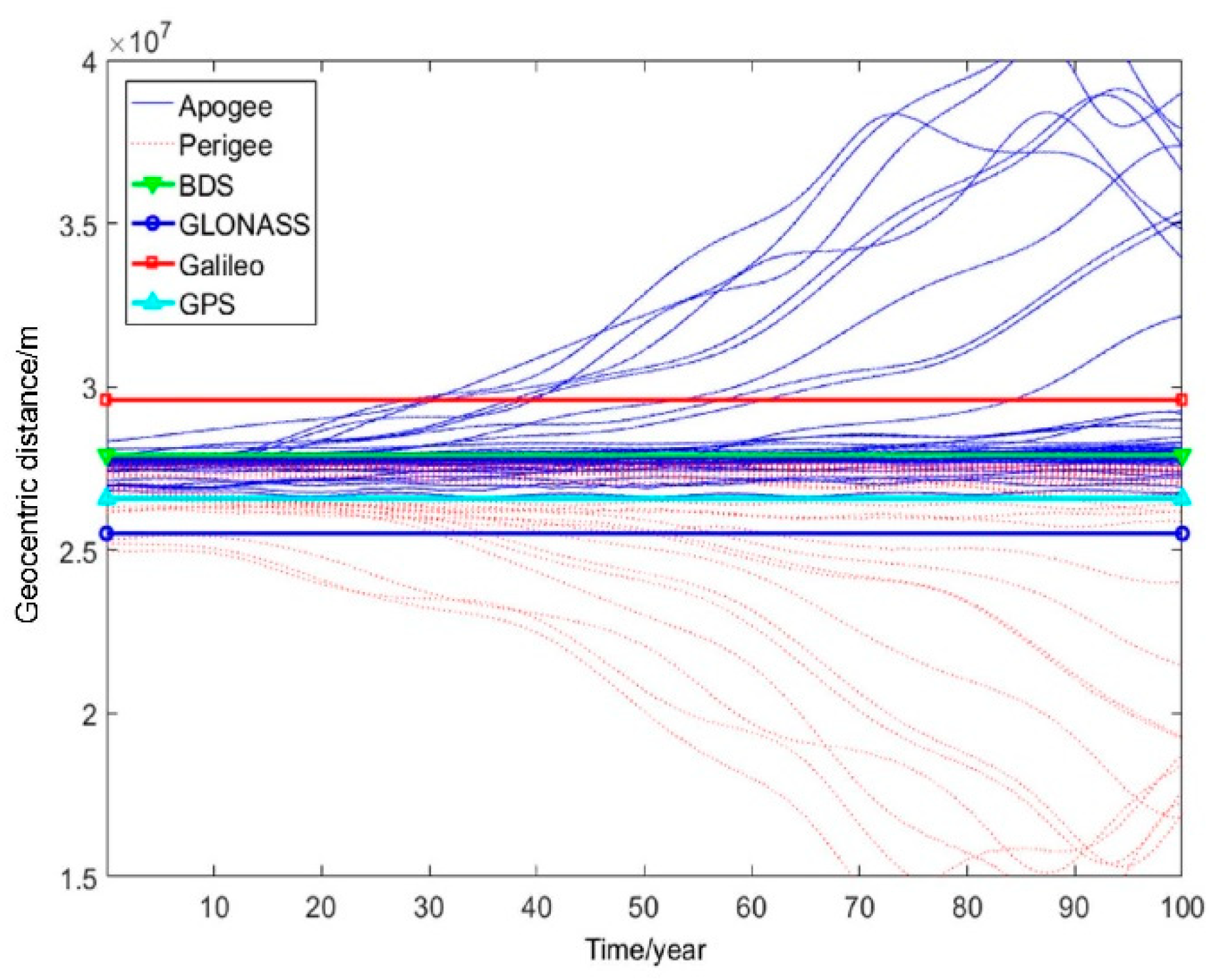
2.3.1. Galileo Constellation

Twenty-six satellites have been launched into orbit. The two satellites launched in the early stage have already deviated from the operational plane and have already crossed the Galileo, BDS, GPS, and GLONASS constellations.

Table 1. Orbital parameters of two Galileo satellites launched in the early stage [22].

NOARD	Apogee Altitude/km	Perigee Altitude/km
40128	26,255	16,944
40129	26,251	16,947

shows the orbital parameters of the two Galileo satellites launched in the early stage.

The long-term evolutions of 24 other Galileo satellites are propagated. Figure 4 shows the orbital variations over 100 years.

From the above graph we can see that the orbits of the 24 Galileo satellites are relatively safe; they will not intersect with other GNSS constellations over the next 100 years.

The spent upper stages of the Galileo system mainly include FREGAT R/B and ARIANE 5 R/B. In the early stage, the upper stages were usually disposed of by raising the orbital altitude. In the year after 2016, the upper stages have typically been disposed of by reducing the orbital altitude. The orbit of the upper stage numbered 40130 has already crossed over into the Galileo, BDS, GPS, and GLONASS constellations.

Table 2. Orbital parameters of the upper stage numbered 40130 [22].

NOARD	Apogee Altitude/km	Perigee Altitude/km
40130	26,090	13,500

shows the orbital parameters of the upper stage numbered 40130.

The long-term evolutions of other spent upper stages are propagated. Figure 5 shows the orbital variations over 100 years.

The initial eccentricity of Galileo is small, and the abandoned orbit of the upper stages is stable and rarely crosses the orbit region of Galileo and other navigation constellations. As shown in Figure 5, the orbits of Galileo spent upper stages are relatively safe; they will not intersect with the Galileo operational orbit, as well as the other GNSS constellations, over the next 100 years.

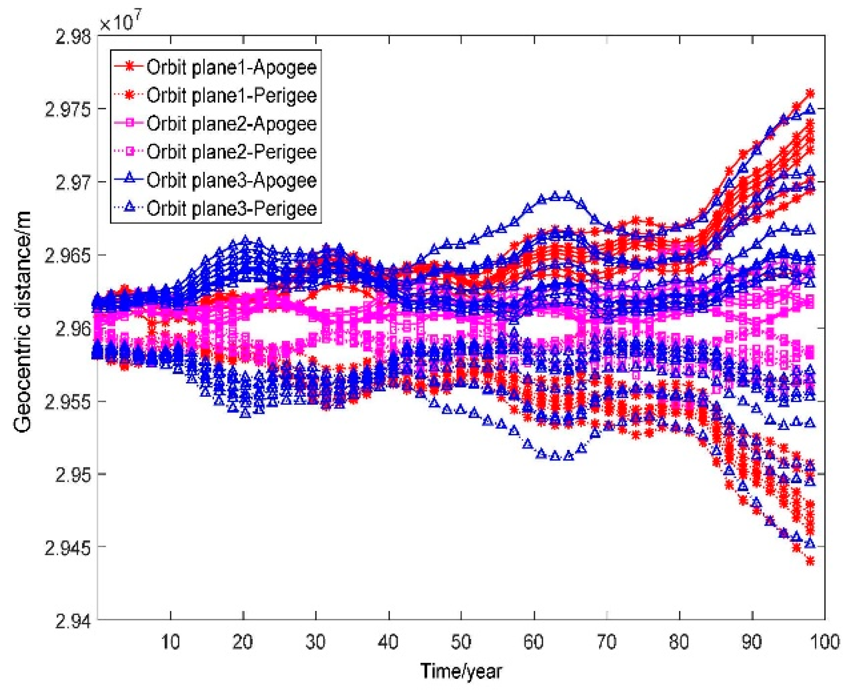
2.3.2. BDS Constellation

Of the twenty-eight MEO satellites that have been launched into orbit, one satellite has already deviated from the operational plane. The long-term evolutions of other twenty-seven satellites are investigated; Figure 6 shows the orbital variations of BDS satellites over the next 100 years.

As shown in Figure 6, the orbits of the 27 BDS satellites are relatively safe. The initial eccentricity of one satellite is relatively large, and it grows to 0.025 after 100 years. However, it still does not intersect with other GNSS constellations over the next 100 years. Therefore, BDS MEO satellites have good stability over the next 100 years.

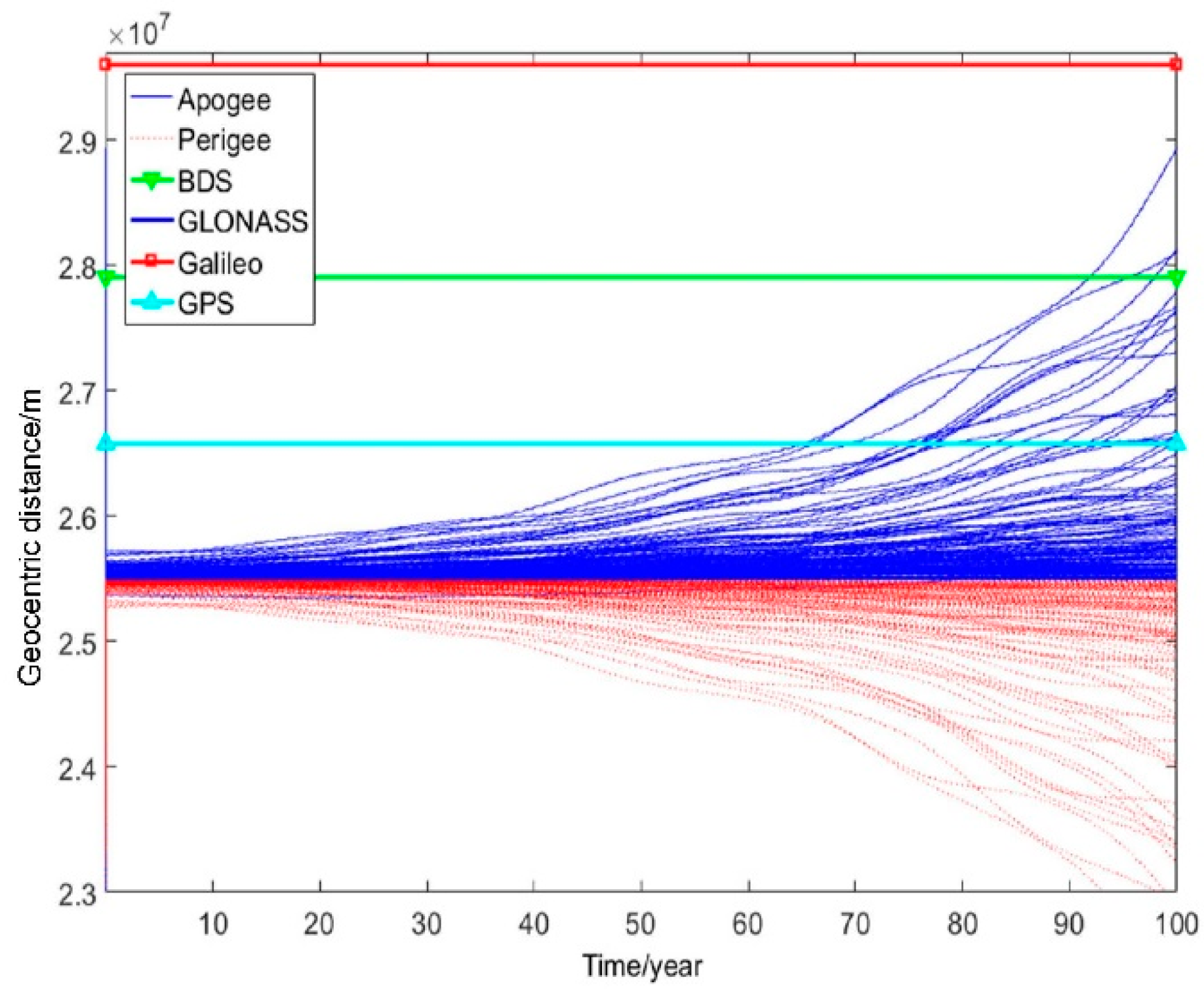
2.3.3. GPS Constellation

Seventy-five GPS satellites have been launched into orbit, of which 31 are in operation. The long-term evolutions of the 31 operational satellites were propagated. Figure 7 shows the orbital variations over the next 100 years.

As shown in Figure 7, due to a slightly large initial eccentricity, the perigees of several operational satellites will intersect with the GLONASS constellation after approximately 25 years, with the BDS constellation after approximately 40 years, and with the Galileo constellation after approximately 80 years. Thus, GPS satellites will be less stable during the next 100 years.

Figure 8 shows the orbital variations of disposed GPS satellites over the next 100 years.

As depicted in Figure 8, the perigees of several disposed satellites have already intersected with the GLONASS and BDS constellations and will intersect with the Galileo constellation after approximately 40 years.

The spent upper stages of GPS mainly include DELTA 4 R/B and ATLAS 5 CENTAUR R/B. The orbit of several spent upper stages is raised. The long-term evolutions of other spent upper stages were propagated. Figure 9 shows the orbital variations over the next 100 years.

As shown in Figure 9, many of the spent GPS upper stages have already intersected with the BDS constellation and will intersect with the GLONASS and Galileo constellations after approximately 45 years.

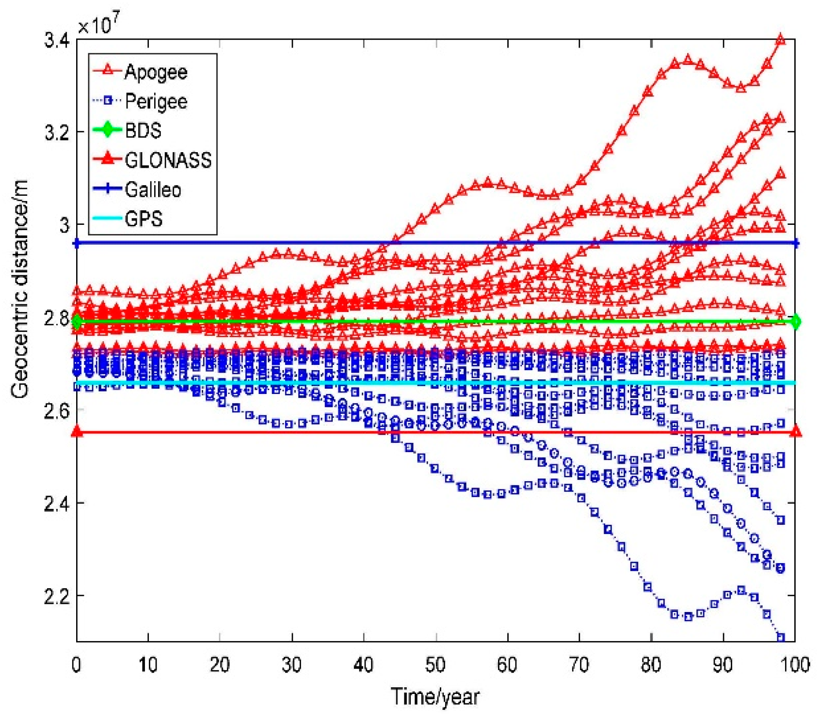
2.3.4. GLONASS Constellation

One hundred and thirty-four GLONASS satellites have been launched into orbit, of which 23 satellites are in operation. The long-term evolutions of the 23 operational satellites were propagated. Figure 10 shows the orbital variations over the next 100 years.

As shown in Figure 10, due to the small initial eccentricity, the eccentricity grows slowly over the next 100 years. The orbit of the operational satellites will intersect with the GPS constellation after approximately 95 years.

Figure 11 shows the orbital variations of the disposed GLONASS satellites over the next 100 years.

As illustrated in Figure 11, the orbit of several disposed satellites will intersect with the GPS constellation after approximately 65 years and with the BDS constellation after approximately 95 years but will not intersect with the Galileo constellation over the next 100 years.

The spent upper stages of GLONASS mainly include SL-12 R/B(2) and FREGAT R/B. The spent upper stages were left in orbit in the early stage. In the years after 2011, the upper stages have usually been disposed of by raising the orbital altitude. The orbital evolution of the GLONASS spent upper stages over the next 100 years was carried out, and the evolution results of its apogee and perigee geocentric distances are shown in Figure 12.

As shown in Figure 12, GLONASS spent upper stages will intersect with the GPS constellation after approximately 40 years and with the BDS constellation after approximately 80 years.

3. End-of-Life Disposal Analysis for BDS MEO Satellites

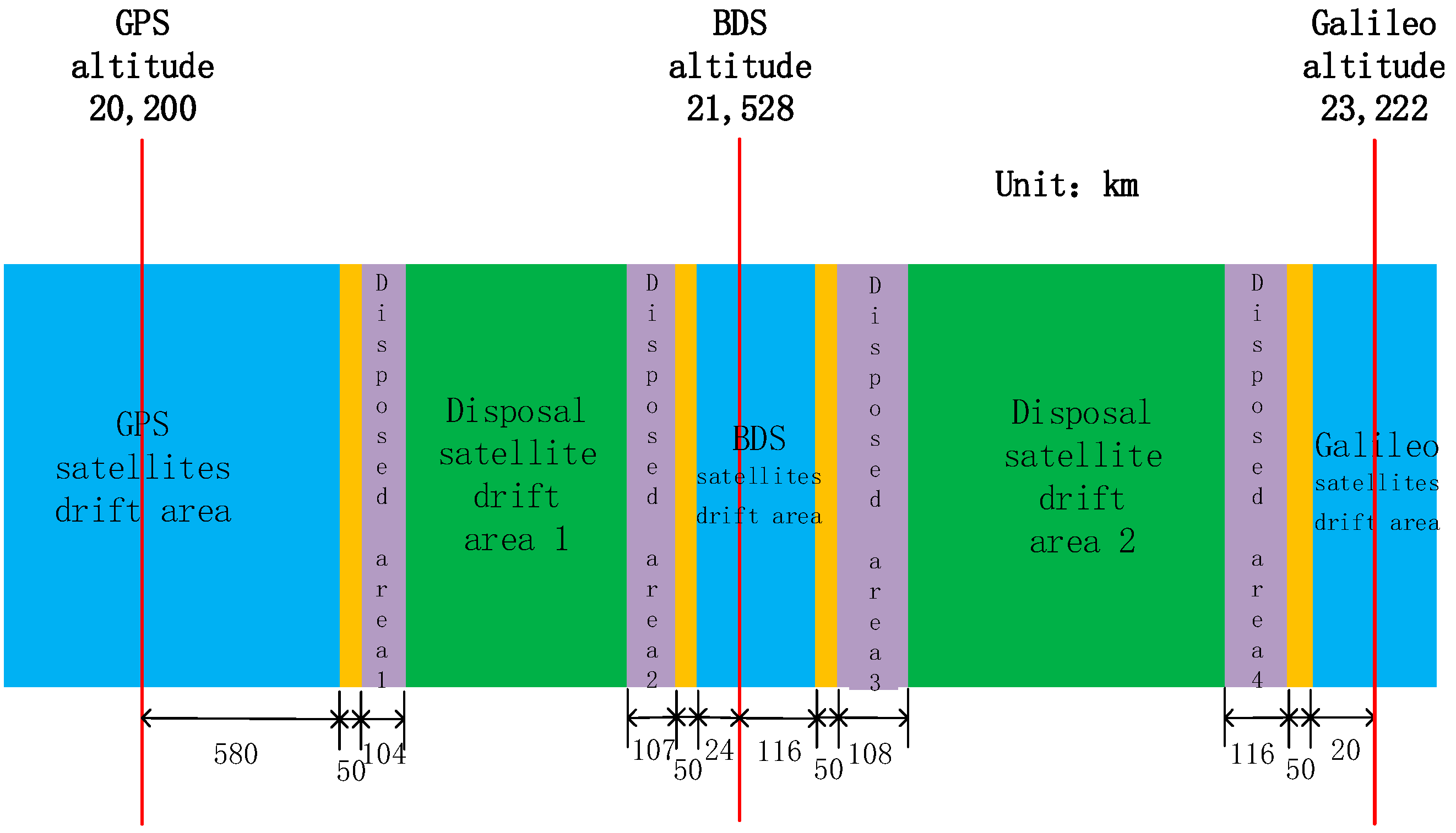
3.1. Distribution Status of the Space Objects in MEO Region

Based on the TLEs obtained from Reference [22], the distributions of navigation satellites and spent upper stages in the MEO region were analyzed. Figure 13 shows the distributions of the navigation satellites.

As shown in Figure 13, several disposed GPS satellites have already crossed into the BDS and GLONASS regions and have a peak value of space object density near the BDS operational orbit. Most of the disposed GLONASS are left in the operational orbit; the space object density near the GLONASS operational orbit is relatively large.

Figure 14 shows the distributions of spent upper stages.

As demonstrated in Figure 14, most of the spent upper stages of GPS, BDS, and Galileo are abandoned above their operational orbit. Meanwhile, most of the spent upper stages of GLONASS are left near its operational orbit.

Table 3. Deorbit statuses of the retired navigation satellites and the spent upper stages [22].

Constellation	Deorbit Navigation		Deorbit Upper Stages
	Number	Apogee/km	Number	Apogee/km
GPS	>30	+350~1700	12	+600~1900
GLONASS	—	—	20	0~+00
Galileo	2	+120~+600	8	+350~+2900
BDS	1	+300	7	+200~+6000

shows the deorbit statuses of the retired navigation satellites and the spent upper stages.

3.2. Orbit Manoeuvre Model

The changes in the right ascension of the ascending node and orbital inclination usually consume large amounts of fuel. Therefore, the disposal orbit and the operational orbit are usually in the same orbital plane, and dual-impulse transfer is convenient. Dual-impulse apsidal rotation is the best control pattern for coplanar elliptical maneuvers. The simplified dual-impulse symmetrical control was adopted. Figure 15 shows its schematic.

The total $\Delta \upsilon$ is expressed as follows:

$$\begin{array}{l}\Delta \upsilon =\Delta {\upsilon }_1+\Delta {\upsilon }_2={\{{[{(v_r)}_{T1}-{(v_r)}_{1T}]}^2+{[{(v_t)}_{1T}-{(v_t)}_{T1}]}^2\}}^{\frac{1}{2}}\\ +{\{{[{(v_r)}_{2T}-{(v_r)}_{T2}]}^2+{[{(v_t)}_{2T}-{(v_t)}_{T2}]}^2\}}^{\frac{1}{2}}\end{array}$$

(10)

where $\Delta {\upsilon }_1$ is the first velocity increment, $\Delta {\upsilon }_2$ is the second velocity increment.

The orbit velocity of the initial orbit, transfer orbit and target orbit should satisfy the following restrictions:

$$\{\begin{array}{l}{\nu }_r=\dot{r}=\sqrt{\frac{\mu }{p}}e\sin f\\ {\nu }_t=r\dot{f}=\sqrt{\frac{\mu }{p}}\left(1+e\cos f\right)\end{array}$$

(11)

where ${\nu }_r$, ${\nu }_t$ are the radial velocity and the circumferential velocity, respectively, which can be divided as radial velocity and along-track velocity. $\mu$ is the Earth gravity constant, $p$ is the semi-latus rectum, $e$ is the orbital eccentricity, and $f$ is the true anomaly.

Equation (11) is a quadratic function of $f_{1T}$ and $f_{T1}$:

$$\Delta v=F(f_{T1},f_{1T})$$

(12)

where $f_{1T}$ is the true anomaly of the first maneuver point, $f_{T1}$ is the selected orbital parameters.

The optimal index is $\underset{f1\mathrm{T}}{\min }\left[\underset{f\mathrm{T}1}{\min }(\Delta \upsilon )\right]$, which can be used to select the optimal maneuvre point and minimize the velocity increment.

3.3. Disposal Orbit Optimization Models

3.3.1. Object Function

The disposal orbit should be kept stable for as long as possible, and the eccentricity should grow slowly in a long-time evolution. Fuels are limited for MEO satellites; hence, the fuel used for maneuvering should be minimized to prolong the working time of the satellites. The optimization model is expressed as follows:

$$\{\begin{array}{l}F=C_1\Delta R_a+C_2\Delta R_p+C_3\Delta V+C_4\Delta e\\ R_a=a\times (1+e)\\ R_p=a\times (1-e)\\ \Delta R_a=h_{\max }-R_a{}_{\max }\\ \Delta R_p=R_{p\min }-h_{\min }\\ \Delta e=e_{\max }-e_{\mathrm{init}}\end{array}$$

(13)

where $C_1$, $C_2$, $C_3$, and $C_4$ are weight coefficients, respectively. $R_a{}_{\max }$ is the maximum apogee of the disposal orbit in 200 years, $h_{\max }$ is the upper bound of the disposal orbit, $R_{p\min }$ is the minimum perigee of the disposal orbit in 200 years, $h_{\min }$ is the lower bound of the disposal orbit, $\Delta V$ is the velocity increment, and $\Delta e$ is the difference between the maximum eccentricity in 200 years and the initial eccentricity.

The orders of $\Delta R_a$, $\Delta R_p$, $\Delta V$, and $\Delta e$ have big differences, therefore, they are normalized as $\Delta R_a{}_{\mathrm{norm}}$, $\Delta R_p{}_{\mathrm{norm}}$, $\Delta V_{\mathrm{norm}}$, and $\Delta e_{\mathrm{norm}}$, respectively.

The final object function is expressed as follows:

$$F=C_1\Delta R_a{}_{\mathrm{norm}}+C_2\Delta R_p{}_{\mathrm{norm}}+C_3\Delta V_{\mathrm{norm}}+C_4\Delta e_{\mathrm{norm}}$$

(14)

3.3.2. Bounds for Disposal Region of BDS MEO Satellites

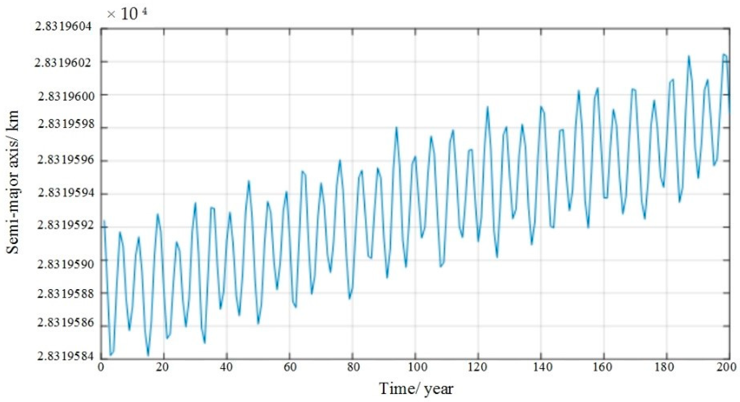
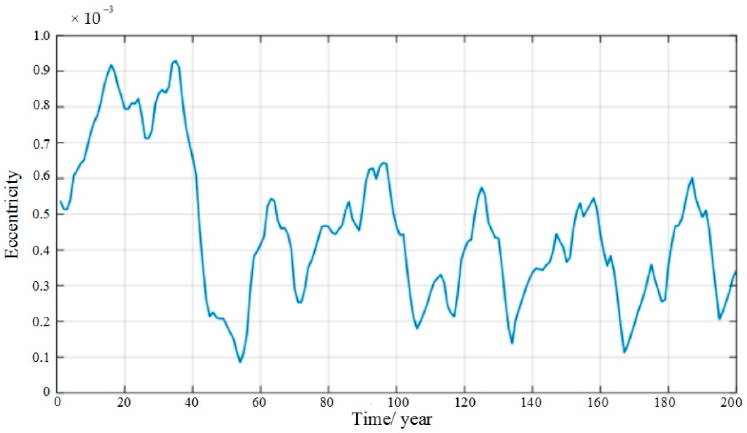
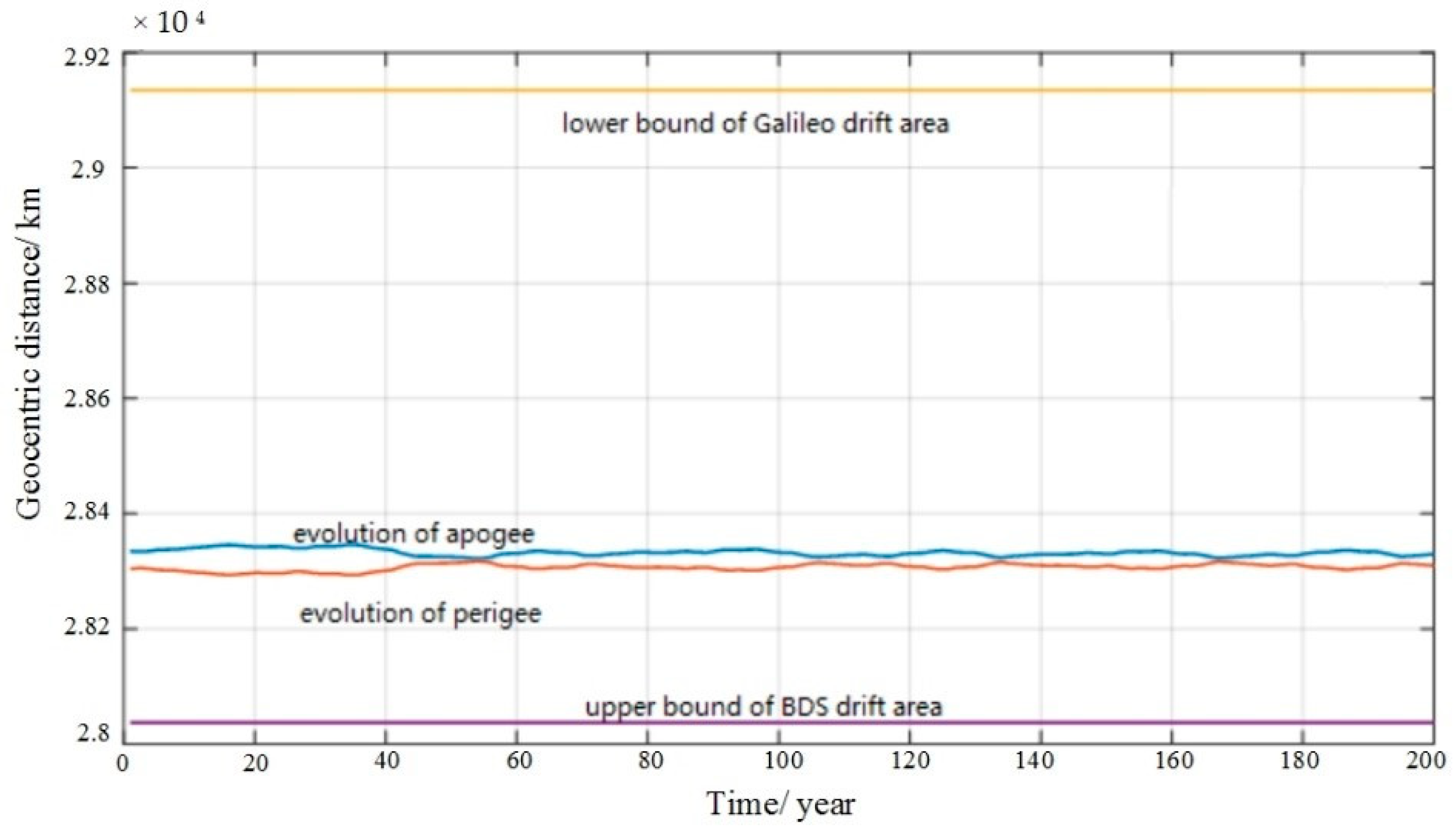
The right ascension of the ascending node and the orbital inclination are usually not changed during the disposal process. Therefore, the initial semimajor axis, eccentricity, and the argument of perigee are analyzed.

The GPS constellation has the closest range relative to the BDS constellation, which has a lower altitude of 1326 km. The Galileo constellation has the second closest range relative to the BDS constellation, which has a higher altitude of 1694 km. The orbital altitude of the end-of-life BDS MEO satellites can be increased or reduced, which has a relatively large range.

The altitude bounds of GPS, Galileo, and BDS were analyzed on the basis of up-to-date orbit observation data. The drift regions of the GPS, Galileo, and BDS satellites in the MEO, the allowed drift regions of the disposal satellites, and the band regions suitable for the selection of the graveyard orbits were formulated with the data, and the relationship between them is shown in Figure 16.

The satellite drift areas are restricted by the following equations:

$$\begin{array}{l}{R}_{\max }=R{a}_{\max }+50\mathrm{km}\\ R_{\min }=R{p}_{\min }-50\mathrm{km}\end{array}$$

(15)

where $R_{\max }$ is the upper bound of the drift area, $R_{\min }$ is the lower bound of the drift area, $R{a}_{\max }$ is the maximum apogee of all the satellites in the constellation, $R{p}_{\min }$ is the minimum perigee of all the satellites in the constellation, 50 km is proposed considering the measurement and control error of the BDS MEO satellites. The upper bound of the GPS constellation is 27,120 km, the lower bound of the BDS MEO constellation is 27,773 km and the upper bound of the BDS MEO constellation is 28,037 km, and the lower bound of the Galileo MEO constellation is 29,135 km.

3.4. Simulations

3.4.1. Raising Orbit Scenario

The BDS M3 satellite is regarded as an example. Its orbit is raised after retirement. Figure 17 shows the variations in the semimajor axis of the optimal disposal orbit.

Figure 18 depicts the variations in the eccentricity of the optimal disposal orbit.

Figure 19 shows the variations in the minimum perigee and the maximum apogee of the optimal disposal orbit.

As shown in Figure 17, the semimajor axis of the optimal disposal orbit varies from 28,319.583 km to 28,319.604 km over 200 years. From Figure 18, the eccentricity of the optimal disposal orbit varies from 0.000002 to 0.001029 over 200 years. From Figure 19, the perigee of the optimal disposal orbit varies from 28,290.446 km to 28,319.537 km over 200 years, and the apogee of the optimal disposal orbit varies from 28,319.646 km to 28,348.729 km over 200 years. The closest range relative to the upper bound of the BDS satellite drift area is 253.446 km, and the closest range relative to the lower bound of the Galileo satellite drift area is 786.271 km.

3.4.2. Reducing Orbit Scenario

The BDS M3 satellite is regarded as an example. Its orbit is reduced after retirement. Figure 20 shows the variations in the semimajor axis of the optimal disposal orbit.

Figure 21 demonstrates the variations in the eccentricity of the optimal disposal orbit.

Figure 22 shows the variations in the minimum perigee and the maximum apogee of the optimal disposal orbit.

As shown in Figure 20, the semimajor axis of the optimal disposal orbit varies from 27,345.444 km to 27,345.468 km over 200 years. From Figure 21, the eccentricity of the optimal disposal orbit varies from 0.000001 to 0.000976 over 200 years. From Figure 22, the perigee of the optimal disposal orbit varies from 27,318.756 km to 27,345.430 km over 200 years, and the apogee of the optimal disposal orbit varies from 27,345.479 km to 27,372.136 km over 200 years. The closest range relative to the lower bound of the BDS satellite drift area is 400.86 km, and the closest range relative to the upper bound of the GPS satellite drift area is 198.756 km.

Figure 19 and Figure 22 depict that raising the orbit has a larger safe distance relative to reducing the orbit. The optimal orbit altitude rises by 413.591 km. The orbit transfer $\Delta v$ required is 21.208 m/s.

4. Conclusions

In this study, the perturbation forces, including the Earth’s nonspherical perturbations, luni-solar perturbations, and solar radiation pressure perturbations, of space objects in the MEO region were analyzed. Perturbation models of the long-term evolution were established by adopting equinoctial elements, which avoided the singularity and greatly enhanced the computation efficiency.

On the basis of the analysis, the orbits of the operational satellites, disposed satellites, and spent upper stages over the next 100 years were simulated, and their orbit intersection time was put forward. The simulation results showed that the evolution orbit intersection with the other GNSS constellations of operational GPS satellites, disposed satellites, and spent upper stages was relatively evident and that other GNSS constellations are relatively stable. The intersection of the orbits does not necessarily mean that the satellites will collide, but this relatively increases the collision probability. To sustain the safety of the MEO region, there should be a focus on the orbit altitude and eccentricity. The appropriate disposal of decommissioned satellites and spent upper stages may reduce the collision risk of space objects in the MEO region. The decommissioned satellites and spent upper stages can be kept in the stable orbits of the MEO region or re-enter the atmosphere, which makes the MEO region safe and sustainable.

Furthermore, the distribution status of navigation satellites and spent upper stages in the MEO region was analyzed, a dynamic model and the orbital maneuver for disposal orbits were established, an optimization model for disposal orbits was proposed, and the bounds for the disposal region for BDS MEO satellites were put forward. Lastly, two disposal cases for end-of-life BDS MEO satellites, namely, upraising and reducing the orbit, are simulated. Furthermore, the results showed that the two disposal orbits would be stable in 200 years, but raising the orbit at the end of life has a relatively larger safe distance.

References

1. Global Navigation Satellite Systems. Available online: https://www.glonass-iac.ru/index.php (accessed on 9 March 2022).
2. Scala, F.; Colombo, C.; Gkolias, I. Design of disposal orbits for high altitude spacecraft with a semi-analytical model. In Proceedings of the 18th Australian Aerospace Congress, Melbourne, Australia, 24–28 February 2019; pp. 1–21. [Google Scholar]
3. Zhang, B. Research on Space Debris Environment Long-Term Evolution Modeling and Its Safety Problem. Ph.D. Thesis, National University of Defense Technology, Changsha, China, 2017. [Google Scholar]
4. Métris, G.; Exertier, P. Semi-analytical theory of the mean orbital motion. Astron. Astrophys. 1995, 294, 278–286. [Google Scholar]
5. Valk, S.; Lemaître, A.; Deleflie, F. Semi-analytical theory of mean orbital motion for geosynchronous space debris under gravitational influence. Adv. Space Res. 2009, 43, 1070–1082. [Google Scholar] [CrossRef]
6. Lara, M.; San-Juan, J.F.; López-Ochoa, L.M.; Cefola, P. Long-term evolution of Galileo operational orbits by canonical perturbation theory. Acta Astronaut. 2014, 94, 646–655. [Google Scholar] [CrossRef]
7. Valk, S.; Lemaître, A.; Anselmo, L. Analytical and semi-analytical investigations of geosynchronous space debris with high area-to-mass ratios. Adv. Space Res. 2008, 41, 1077–1090. [Google Scholar] [CrossRef]
8. Kirchner, G.; Steindorfer, M.; Wang, P.; Koidl, F.; Kucharski, D.; Silha, J.; Schildknecht, T.; Krag, H.; Flohrer, T. Determination of attitude and attitude motion of space debris, using laser ranging and single-photon light curve data. In Proceedings of the 7th European Conference on Space Debris, Darmstadt, Germany, 18–21 April 2017; pp. 18–21. [Google Scholar]
9. Kucharski, D.; Kirchner, G.; Bennett, J.; Lachut, M.; Sośnica, K.; Koshkin, N.; Shakun, L.; Koidl, F.; Steindorfer, M.; Wang, P. Photon pressure force on space debris TOPEX/Poseidon measured by satellite laser ranging. Earth Space Sci. 2017, 4, 661–668. [Google Scholar] [CrossRef]
10. Yakovlev, M. The “IADC Space Debris Mitigation Guidelines” and supporting documents. In Proceedings of the 4th European Conference on Space Debris, Darmstadt, Germany, 18–20 April 2005; pp. 591–597. [Google Scholar]
11. Chobotov, V. Disposal of spacecraft at end of life in geosynchronous orbit. J. Spacecr. Rockets 1990, 27, 433–437. [Google Scholar] [CrossRef]
12. Chao, C. MEO disposal orbit stability and direct reentry strategy. In Proceedings of the AAS/AIAA Spaceflight Mechanics Meeting, Clearwater, FL, USA, 23–26 January 2000. [Google Scholar]
13. Rossi, A. Resonant dynamics of Medium Earth Orbits: Space debris issues. Celest. Mech. Dyn. Astron. 2008, 100, 267–286. [Google Scholar] [CrossRef]
14. Chao, C.; Gick, R.A. Long-term evolution of navigation satellite orbits: GPS/GLONASS/GALILEO. Adv. Space Res. 2004, 34, 1221–1226. [Google Scholar] [CrossRef]
15. Domınguez-González, R.; Sánchez-Ortiz, N.; Cacciatore, F.; Radtke, J.; Flegel, S. Disposal strategies analysis for MEO orbits. In Proceedings of the 64th International Astronautical Congress, Beijing, China, 23–27 September 2013. [Google Scholar]
16. Alessi, E.M.; Rossi, A.; Valsecchi, G.; Anselmo, L.; Pardini, C.; Colombo, C.; Lewis, H.; Daquin, J.; Deleflie, F.; Vasile, M. Effectiveness of GNSS disposal strategies. Acta Astronaut. 2014, 99, 292–302. [Google Scholar] [CrossRef] [Green Version]
17. Radtke, J.; Domínguez-González, R.; Flegel, S.K.; Sánchez-Ortiz, N.; Merz, K. Impact of eccentricity build-up and graveyard disposal strategies on MEO navigation constellations. Adv. Space Res. 2015, 56, 2626–2644. [Google Scholar] [CrossRef]
18. Armellin, R.; San-Juan, J.F. Optimal Earth’s reentry disposal of the Galileo constellation. Adv. Space Res. 2018, 61, 1097–1120. [Google Scholar] [CrossRef]
19. Armellin, R.; San-Juan, J.F.; Lara, M. End-of-life disposal of high elliptical orbit missions: The case of INTEGRAL. Adv. Space Res. 2015, 56, 479–493. [Google Scholar] [CrossRef] [Green Version]
20. Mistry, D.; Armellin, R. The design and optimisation of end-of-life disposal manoeuvres for GNSS spacecraft: The case of Galileo. In Proceedings of the 66th International Astronautical Congress, Jerusalem International Convention Cente, Jerusalem, Israel, 12–16 October 2015. [Google Scholar]
21. Hu, M.; Fan, L.; Yang, M. Optimal disposal orbit design for MEO navigation constellations. In Proceedings of the 67th International Astronautical Congress, Guadalajara, Mexico, 26–30 September 2016. [Google Scholar]
22. Hu, M.; Xu, J.; Li, J.; Wang, X. Long-term evolution safety analysis and disposal orbit design method of BDS MEO satellite orbits. In Proceedings of the 69th International Astronautical Congress, Bremen, Germany, 1–5 October 2018. [Google Scholar]
23. Skoulidou, D.K.; Rosengren, A.J.; Tsiganis, K.; Voyatzis, G. Medium Earth Orbit dynamical survey and its use in passive debris removal. Adv. Space Res. 2019, 63, 3646–3674. [Google Scholar] [CrossRef] [Green Version]
24. Dominguez-Gonzalez, R. Long-Term Implications of GNSS Disposal Strategies for the Space Debris Environment. In Proceedings of the 7th European Conference on Space Debris, Darmstadt, Germany, 18–21 April 2017. [Google Scholar]
25. Gondelach, D.J.; Armellin, R.; Wittig, A. On the predictability and robustness of Galileo disposal orbits. Celest. Mech. Dyn. Astron. 2019, 131, 60. [Google Scholar] [CrossRef] [Green Version]
26. Liu, H. The Analytical Theory of Space-Based Gravity Measurements and Its Realization Method by Satellite Formation. Ph.D. Thesis, National University of Defense Technology, Changsha, China, 2015. [Google Scholar]
27. Jenkin, A.B.; McVey, J.P.; Sorgeb, M.E. Assessment of time spent in the LEO, GEO, and semi-synchronous zones by spacecraft on long-term reentering disposal orbits. Acta Astronaut. 2021, 193, 579–594. [Google Scholar] [CrossRef]
28. Bordovitsyna, T.; Tomilova, I.; Chuvashov, I. The effect of secular resonances on the long-term orbital evolution of uncontrollable objects on satellite radio navigation systems in the MEO region. Sol. Syst. Res. 2012, 46, 329–340. [Google Scholar] [CrossRef]
29. Cefola, P.; Folcik, Z.; Di-Costanzo, R.; Bernard, N.; Setty, S.; Juan, J. Revisiting the DSST standalone orbit propagator. In Proceedings of the 24th AAS/AIAA Space Flight Mechanics Meeting, Santa Fe, NM, USA, 26–30 January 2014. [Google Scholar]
30. MEO tle. Available online: http://www.space-track.org (accessed on 10 December 2021).
Figure 1. Magnitude of acceleration vs. orbital altitude.
Aerospace 09 00266 g001
Figure 2. Variations of the orbital elements.
Aerospace 09 00266 g002
Figure 3. Equinoctial coordinate system with respect to one direct orbit.
Aerospace 09 00266 g003
Figure 4. Orbital variations of Galileo satellites over 100 years.
Aerospace 09 00266 g004
Figure 5. Orbital variations of Galileo spent upper stages over 100 years.
Aerospace 09 00266 g005
Figure 6. Orbital variations of BDS satellites over 100 years.
Aerospace 09 00266 g006
Figure 7. Orbital variations of GPS operational satellites over 100 years.
Aerospace 09 00266 g007
Figure 8. Orbital variations of GPS disposed satellites over 100 years.
Aerospace 09 00266 g008
Figure 9. Orbital variations of GPS spent upper stages over 100 years.
Aerospace 09 00266 g009
Figure 10. Orbital variations of GLONASS operational satellites over 100 years.
Aerospace 09 00266 g010
Figure 11. Orbital variations of GLONASS disposed satellites over 100 years.
Aerospace 09 00266 g011
Figure 12. Orbital variations of GLONASS spent upper stages over 100 years.
Aerospace 09 00266 g012
Figure 13. Distributions of navigation satellites in the MEO region.
Aerospace 09 00266 g013
Figure 14. Distributions of spent upper stages in the MEO region.
Aerospace 09 00266 g014
Figure 15. Schematic diagram of dual-impulse symmetrical control.
Aerospace 09 00266 g015
Figure 16. Altitude bounds for disposal region of BDS MEO satellites.
Aerospace 09 00266 g016
Figure 17. Variations in the semimajor axis of the optimal disposal orbit.
Aerospace 09 00266 g017
Figure 18. Variations in the eccentricity of the optimal disposal orbit.
Aerospace 09 00266 g018
Figure 19. Variations in the minimum perigee and the maximum apogee of the optimal disposal orbit.
Aerospace 09 00266 g019
Figure 20. Variations in the semimajor axis of the optimal disposal orbit.
Aerospace 09 00266 g020
Figure 21. Variations in the eccentricity of the optimal disposal orbit.
Aerospace 09 00266 g021
Figure 22. Variations in the minimum perigee and the maximum apogee of the optimal disposal orbit.
Aerospace 09 00266 g022