1. Introduction
Regarding air traffic management research, there have been three main objectives of interest: reduce air flight delay, solve air traffic conflicts efficiently and mitigate air space congestion. This work proposes a method to assess the latter.
The operational capacity of a control sector is measured by the maximum number of flights that may cross the sector in a given period. This measurement does not consider the direction of the traffic, treating geometrically structured and disordered traffic in the same way. Thus, in certain situations, a controller may continue to accept traffic even if operational capacity has been reached (structured traffic situation). In other cases, a controller may need to refuse airplanes even though the operational capacity has not been reached (disordered traffic situation). Thus, modeling airspace congestion using the number of airplanes per unit of time is insufficient to reflect the levels of difficulty involved in a traffic situation.
Air traffic control organizes air flows to ensure flight safety and increase the route network’s capacity. In 2019, before COVID-19, about 8500 flights were registered every day over France, which is a crossroad for the whole European airspace. This traffic generates a huge amount of control workload, and the airspace is then divided into elementary sectors which air navigation controllers manage. For several years, a constant increase in air traffic has induced more and more congestion in the control sectors. Two strategies can then be applied to reduce such congestion. The first one consists of adapting the demand to the existing capacity (slot-route allocation, collaborative decision-making, etc.). The second one adapts the capacity to the demand (modification of the air network, new design of the sectorization, new airports, etc.). For the two preceding approaches, the capacity of a sector is measured by the number of aircraft flying across the sector during a given period of time.
This study aims to synthesize a traffic complexity indicator to better quantify the congestion in the air sector, which will be more relevant than a simple number of aircraft independent of the traffic configuration. More precisely, our objective is to build a metric of the intrinsic complexity of the traffic distribution in the airspace, which relates to controller workload. Such metrics must capture the level of disorder (or organization) of any traffic distribution. Usually, metrics are focused on the speed vector distribution, and the associated disorder metric captures only some features of the traffic complexity. The real objective of our work is to build a metric that measures the disorder or organization of trajectories in 4D space (3D for space and 1D for time).
Such complexity metrics are relevant for many applications in the air traffic management area. For instance, when a sectorization is designed [
1], the sectors have to be balanced from the congestion point of view; nowadays, only the number of aircraft is used to reach this objective. Another example where a congestion metric is needed is the traffic assignment [
2,
3] for which an optimal time of departure and a route are searched for each aircraft in order to reduce the congestion in the airspace. The complexity metric may also be used to design new air networks, for dynamic sectoring concepts, defining future ATM concepts (Free Flight), etc. Complexity metrics enable one to qualify and quantify the performance of the air traffic service providers and enable a more objective consultation between airlines and providers.
The work presented in this paper is based on a dynamical systems modeling of air traffic. A dynamical system describes the evolution of a given state vector. If such a vector is given by the position of aircraft , a dynamical system associates a speed vector to each point in the airspace. The key idea is to find a dynamical system that models the observed aircraft trajectories. A trajectory disorder metric can be computed based on this dynamical system modeling. The metric is targeted to measure the intrinsic traffic complexity related to a set of 4D trajectories related to the control workload. Such a control workload encompasses other factors (airspace structure, etc.) that are not considered in the metric computation.
In the first section, this paper will summarize the previous related works. The second section will present a linear dynamical system modeling for which the complexity metric can be represented into a complex coordinate system. It is very easy to identify any speed vector organization pattern in this system. The third section illustrates the computation of such a metric in several traffic situations.
2. Previous Related Works
The airspace complexity is related to the traffic structure and the airspace geometry. Different efforts are underway to measure the whole complexity of the airspace.
Wyndemere Inc. [
4] proposed a measure of the perceived complexity of an air traffic situation. This measure is related to the controller’s cognitive workload with or without knowing the aircraft’s intents. The metric is human-oriented and is therefore very subjective.
Laudeman et al. from NASA [
5] have developed a metric called “Dynamic Density”, which is more quantitative than the previous ones and is based on the flow characteristics of the airspace. The “Dynamic Density” is a weighted sum of the traffic density (number of aircraft), the number of heading changes (>15 degrees), the number of speed changes (>0.02 Mach), the number of altitude changes (>750 ft), the number of aircraft with 3D Euclidean distance between 0–25 nautical miles and the number of conflicts predicted in 25–40 nautical miles. The parameters of the sums have been adjusted by showing different traffic situations to several controllers. B. Sridhar from NASA [
6] has developed a model to predict the evolution of such a metric in the near future. Efforts to define “Dynamic Density” have identified the importance of many potential complexity factors, including structural considerations.
Airspace complexity depends on both structural and flow characteristics of the airspace [
6]. The structural characteristics are fixed for a sector and depend on the spatial and physical attributes of the sector, such as terrain, number of airways, airway crossings and navigation aids. The flow characteristics vary as a function of time and depend on the number of aircraft, the mix of aircraft, weather, the separation between aircraft, etc. A combination of these structural and flow parameters influences the controller workload.
The traffic itself is not enough to describe the complexity associated with an airspace. A few previous studies have attempted to include structural consideration in complexity metrics but have done so only to a restricted degree. For example, the Wyndemere Corporation proposed a metric that included a term based on the relationship between aircraft headings and dominant geometric axis in a sector [
4]. The importance of including structural consideration has been explicitly identified in recent work at Eurocontrol. In a study to identify complexity factors using judgment analysis, “Airspace Design” was identified as the second most crucial factor behind traffic volume [
7]. The impact of the structure on the controller workload can be found in the paper [
8,
9]. These papers demonstrate how the impact of the traffic structure (airways, sectors, etc.) is related to the control workload through several traffic factors dependent on the instantaneous distribution of traffic (clustering, number of aircraft, distance between aircraft, relative speed between aircraft, etc.).
The previous models do not take into account the intrinsic traffic disorder, which is related to the complexity. The first efforts related to disorder can be found in [
10]. This paper introduces metrics based on geometrical properties that measure a traffic pattern’s disorder. Those metrics can extract features on the traffic complexity such as proximity (measures the level of aggregation of aircraft in the airspace), convergence (for close aircraft, this metric measures how strongly aircraft are closer to each other) and sensitivity (this metric measures how the relative distance between aircraft is sensible to the control maneuver). G. Aigoin has extended and refined the geometrical class by using a cluster-based analysis [
11]. Two aircraft are said to be in the same cluster if the product of their relative speed and their proximity (a function of the inverse of the relative distance) is above a threshold. For each cluster, a metric of relative dependence between the aircraft is computed, and the whole complexity of the cluster is then given by a weighted sum of the matrix norm. Those norms give an aggregated measure of the level of proximity of aircraft in clusters and the associated convergence. From the cluster matrix, it is also possible to compute the difficulty of a cluster (it measures how hard it is to solve a cluster). Multiple clusters can exist within a sector, and their interactions must also be considered. A measure of this interaction has been proposed by G. Aigoin [
11]. This technique allows multiple complexity metrics to be developed, such as average complexity, maximum and minimum cluster complexities and complexity speeds.
Another approach based on fractal dimension has been proposed by S. Mondoloni and D. Liang in [
12]. Fractal dimension is a metric comparing traffic configurations resulting from various operational concepts. It separates, in particular, the complexity due to sectorization from the complexity due to traffic flow features. The dimension of geometrical figures is well known: a line is of dimension 1, a rectangle of dimension 2, etc. The application of this concept to the air route analysis consists in computing the fractal dimension of the geometrical figure composed of existing air routes. Fractal dimension provides information on the number of degrees of freedom used in the airspace: a higher fractal dimension indicates more degrees of freedom. Therefore, the fractal dimension measures the geometrical complexity of a traffic pattern.
Some new geometrical metrics have been developed in [
13], which are able to capture the level of disorder or the level of organization for some traffic patterns. For instance, in an artificial roundabout moving, the speed vectors are very different even if the global moving is fully organized without any changes in the relative distance between aircraft. The covariance and the Koenig metrics have been developed to capture those features. The first one is able to identify the disorder or organization of translation movements. The second one identifies organized curl moving.
In [
10], another approach based on the nonlinear dynamical system modeling of the air traffic uses the topological entropy as a measure of the disorder of the traffic pattern. This approach represents the traffic’s structure more faithfully, but requires a lot of computation for establishing the metric. First, the non-linear dynamical system is adjusted to the observations in order to build the associated vector field. Then, Lyapunov exponents are computed in order to characterize the overall properties of the vector field. When an exponent has a high value, it demonstrates a high sensitivity to initial conditions, meaning the situation is difficult to predict. In this case, the traffic situation presents a high level of disorder. Unfortunately, this metric is not able to take uncertainties into account, which is the case when one wants to predict congestion in the near future.
We propose in this paper an approximation of such a metric based on the linear dynamical system, which measures the local disorder of a set of trajectories in the neighborhood of a given aircraft at a given time. This approximation is much faster to compute and can take into account uncertainties of the future position of aircraft, which is not possible with the nonlinear dynamical system framework described in [
10].
3. Metric Description (Linear Dynamical System Modeling)
The investigated indicator will be linked to the air traffic modeling by a linear dynamical system, yielding an intrinsic measure of complexity of the geometry of the traffic. This enables one to identify different structures of organization of the aircraft speed vectors such as translation, curve organizations, divergence, convergence, or a mix of them.
3.1. Model
The key idea of this metric is to model the set of aircraft trajectories by a linear dynamical system. A dynamical system models a vector field by a set of differential equations, which describes and controls the evolution of a given state vector and is defined by the following equation:
is the state vector of the system:
In this equation, we only consider the observations’
x and
y components, as air traffic controllers see two dimension speed vectors on their screens. Moreover, the metric will be computed for each flight level in a given airspace. Equation (
1) associates a speed vector
with each point in the state space
. This synthesis is a particular vector field. The average behavior of this vector field is given by the vector
and the linear mapping between the speed vector
and the position vector
is given by matrix
. Therefore, the coefficients of matrix
and vector
determine the mode of evolution of the system in relation to its dynamics.
More precisely, the eigenvalues of this matrix will determine the behavior of the system and will be used to obtain the complexity metric. The properties and relevance of these eigenvalues will be explained in
Section 3.3.
First, we focus on defining and modeling the linear dynamical system that will allow us to obtain matrix
. Our problem therefore consists of determining the dynamical model that is closest to the observations: Those observation are extracted from the radar trackers (positions and speeds of aircraft at a given time). We then consider that for each aircraft, we have set position
and speed measures
at some consecutive time stamps
i:
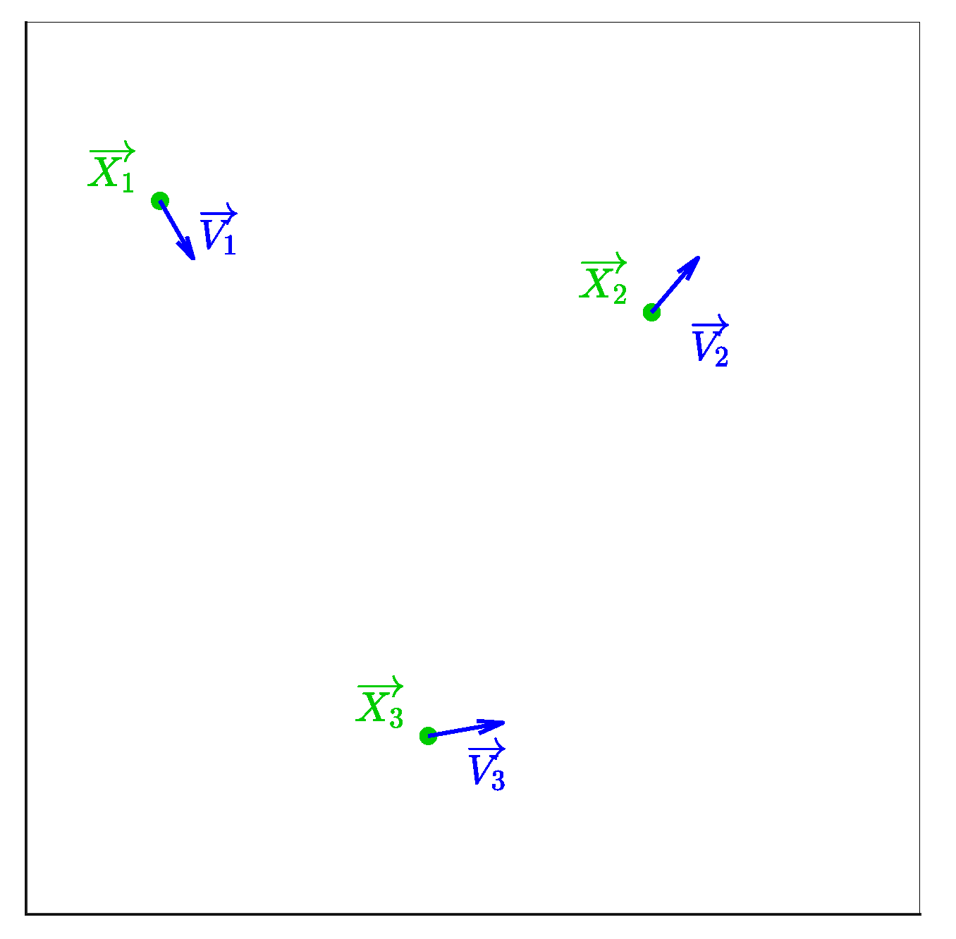
An example of such observations is given on
Figure 1, for which the aircraft observations are represented by the blue arrows.
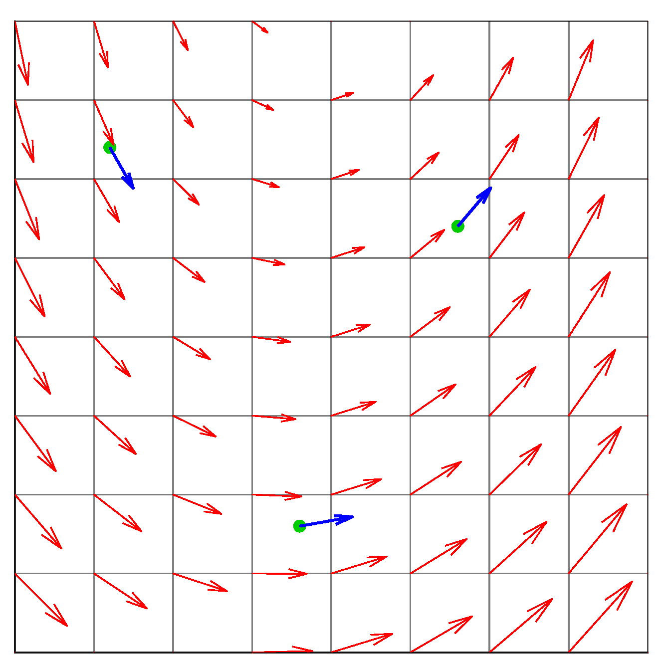
We thus wish to find the vector field described by a linear equation
that is best fitted to our observations. To illustrate this aspect, we construct a grid over the airspace (see
Figure 2) on which we carry out a regression of a vector field that minimizes the error between the model and the observations. In order to use matrix forms, we rewrite Equation (
1) as
, introducing the following matrices:
where
and
n represents the number of observations at a given instant (number of aircraft present in a sector at a given instant).
3.2. Regression
The dynamical system has to be adjusted with the minimum error based on the aircraft observations (positions and speed vectors). This fitting has been performed with a Least Mean Square minimization (LMS) method [
14]. For each considered aircraft
i, it is supposed that position
and speed vector
are given. We then construct an error criterion
E, between the dynamical system model and the observation, based on a norm (Euclidean, in our case), which should be minimized in relation to matrix
and vector
, and therefore in relation to matrix
, which represents the parameters of the model:
E minimization is the same as minimization: .
The derivative of such expression with respect to
is given by:
E is the minimum when:
⇒
then:
On the right side, we recognize the pseudo-inverse of matrix
:
In some situations,
is not invertible, and the computation of the
is not possible by using such an equation. In this case, the classical Singular Value Decomposition (SVD) trick is applied:
where
is a diagonal matrix containing the singular values (only the significant singular values are inverted in this formula in order to control the conditioning of the algorithm).
Based on
, the matrix
is extracted for which an eigenvalue decomposition is computed:
The diagonal matrix contains the eigenvalues. When such eigenvalues have positive real parts, the system is in expansion mode, and when they are negative, the system is in contraction mode.
In addition, the vector represents the global tendency of the vector field.
3.3. Properties of Eigenvalues
The eigenvalues of matrix describe and summarize the evolution of the system. These eigenvalues are complex numbers. Their real parts are related to the convergence or the divergence property of the system in the direction of the eigenvector. When such eigenvalues have positive real parts, the system is in expansion mode (produces divergence), and when they are negative, the system is in contraction mode (produces convergence). The absolute value of these real parts is proportional to the level of contraction or expansion of the system: the larger those real parts are in absolute value, the faster the evolution. Furthermore, the imaginary part of the eigenvalues is related to the level of rotation tendency of the system: the tendency of the system to organize itself following a global rotation movement associated with each of the eigen axes. Depending on those eigenvalues, a dynamical system can evolve in contraction, expansion, rotation, or a combination of those three modes.
We will refer to a fully organized traffic pattern when the relative distances between aircraft do not change with time. For such a situation, the traffic is very predictable and very comfortable to address by a controller: the trajectories do not present any difficulties. These patterns are translation, rotation, or both.
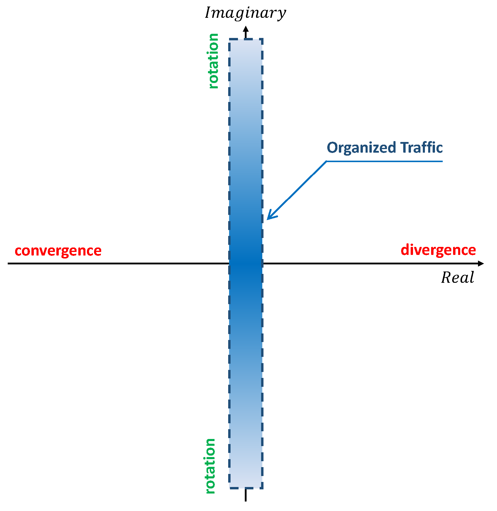
Then, the evolution properties of the system related to the position of the eigenvalues can be summarized in the complex coordinate system (see
Figure 3). In this coordinate system, it is then possible to identify the locus of the eigenvalues of matrix
associated with organized traffic situations: the vertical strip around the imaginary axis. Therefore, organized situations are located around the imaginary axis: when the relative distances between aircraft change slowly with time (this means that the relative speeds between aircraft are close to zero and the traffic has no interaction).
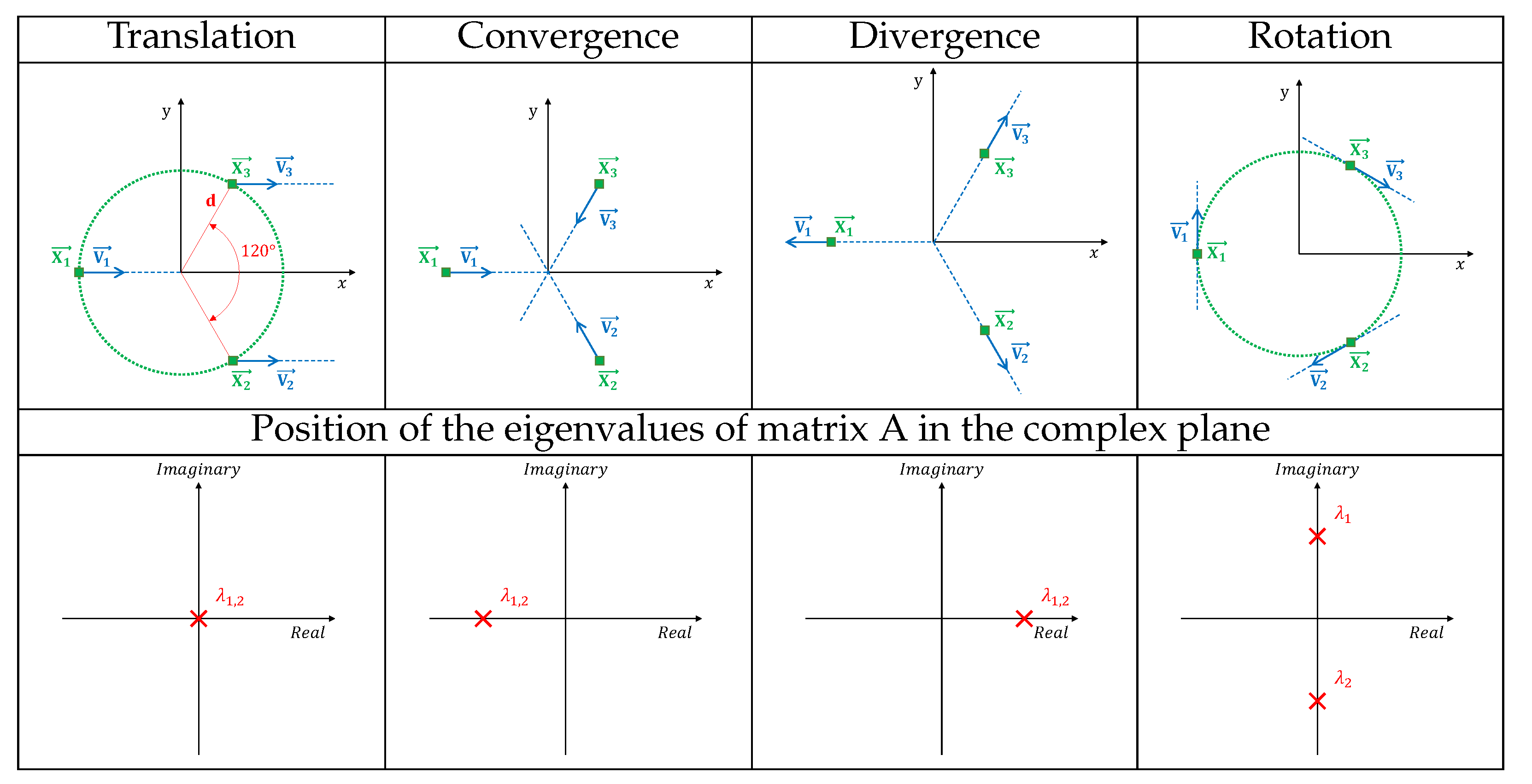
As an example (see
Figure 4), the eigenvalues of matrix
have been calculated for a situation with three aircraft located on a circumference, for which only the orientation of the speed vectors is modified in order to create four traffic situations (pure translation, convergence, divergence and pure rotation). As we can see in
Figure 4, the pure translation and pure rotation are the two organized traffic situations, as they have eigenvalues in the central band of the complex plane.
In the first case, the eigenvalues are null because the aircraft are flying in parallel, representing a translation: the distances between aircraft remain unchanged with time. In the second case, the eigenvalues are real negative; the system evolves in a contraction mode, and the four aircraft are converging: the norms of the relative distances between the aircraft diminish with time. The third situation represents an expansion evolution for which the eigenvalues are real positive, and the aircraft are diverging: the relative distances increase with time. In the two previous situations, the distance between aircraft changes with time, not being organized traffic patterns. The last situation is associated with full imaginary eigenvalues for which the aircraft stay at the same distance from each other in a curl moving. The computation of matrices , vectors and is given for these previous examples:
Looking at
Figure 4, the small squares are the initial positions of aircraft at a given time (this represents the observation given by radar, for instance, with the associated speed vector). As can be observed, the aircraft are initially located on a circumference with a diameter of
. The positions of aircraft two and three are symmetric to the
x-axis. All the speed norms are the same and have been fixed at
. The vector field associated with each one of these four situations is shown in
Figure 5.
3.4. Extension with Uncertainties
If we want to predict complexity in a given airspace, one must be able to take into account future aircraft position uncertainties that are crossing such airspace. Those uncertainties are linked to the wind and temperature encountered by the aircraft along its route. Thus, future positions of aircraft will be represented by a segment along its trajectory arc length in the future. Therefore, as we should account for these uncertainties, it has been considered that at every sample time of the analysis, each aircraft that is within the current modeled airspace area can be ahead or behind its actual position. Then, a time shift is applied to each aircraft (i.e., the reference one and the neighbors) to account for ten forward and ten backward positions. Each shift is equal to twelve seconds, so the most forward and backward positions are separated by two minutes with respect to the reference position.
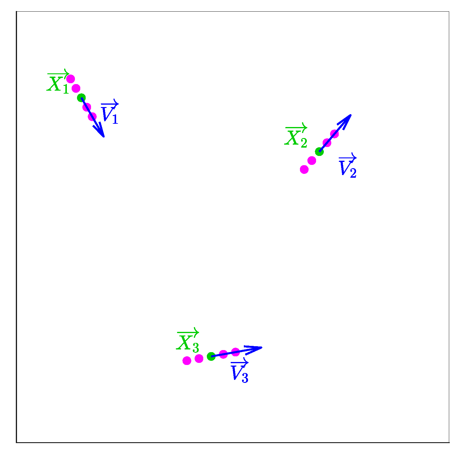
In order to simplify the following figures, we will consider only two shifts in each direction (five positions in total per aircraft) instead of ten only for the visualization of the uncertainties problem in this current section. In
Figure 6, the three aircraft from
Figure 1 are expanded with their corresponding forward and backward positions, applying a time-shift.
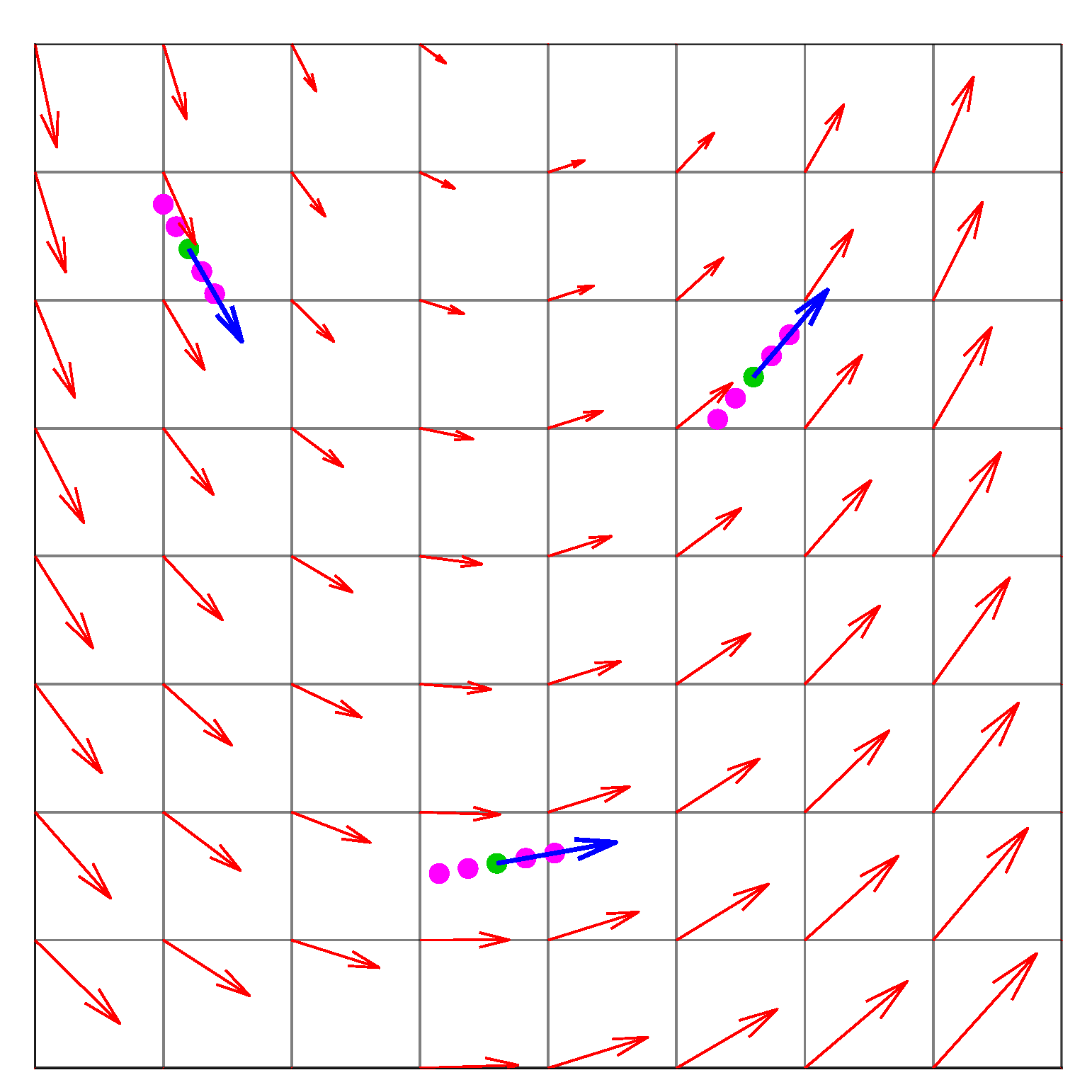
Figure 7 shows the vector field produced by the linear dynamical system corresponding to the above situation.
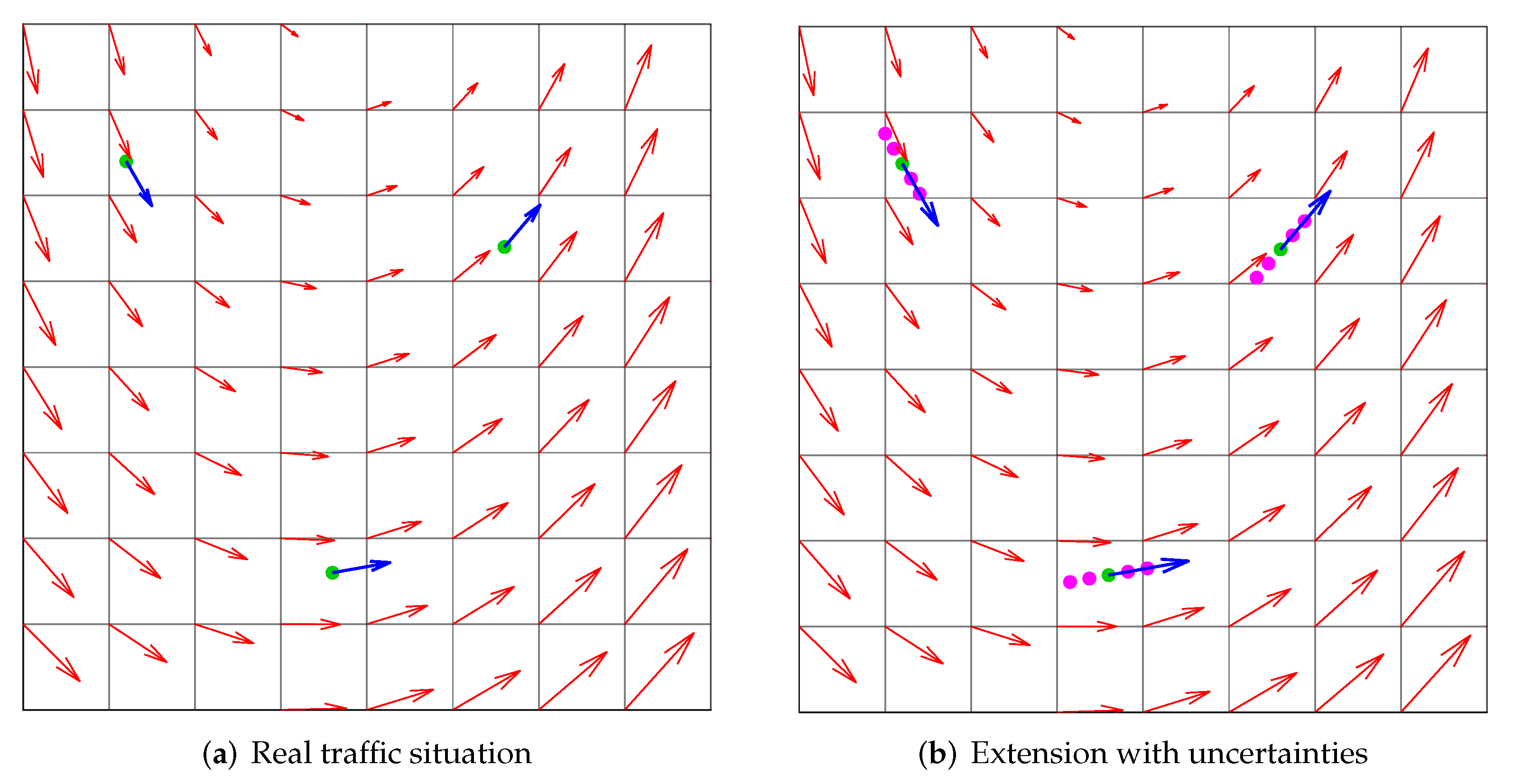
Figure 8 compares the vector field of the situation with and without the uncertainties extension.
This extension will make matrix X larger, as from here on, n would be equal to .
3.5. Metric Computation
The problem will be analyzed within a certain airspace region (e.g., France FIR), thus only the aircraft that are within its boundary are analyzed. By assessing this problem in discrete-time along one aircraft trajectory and considering an area of influence surrounding this aircraft to account for other aircraft, this metric represents the local disorder that is present in the vicinity of an aircraft along its trajectory at each time.
Having obtained matrix and its eigenvalues, the metric is built by summing the negative real part of such eigenvalues hereinafter.
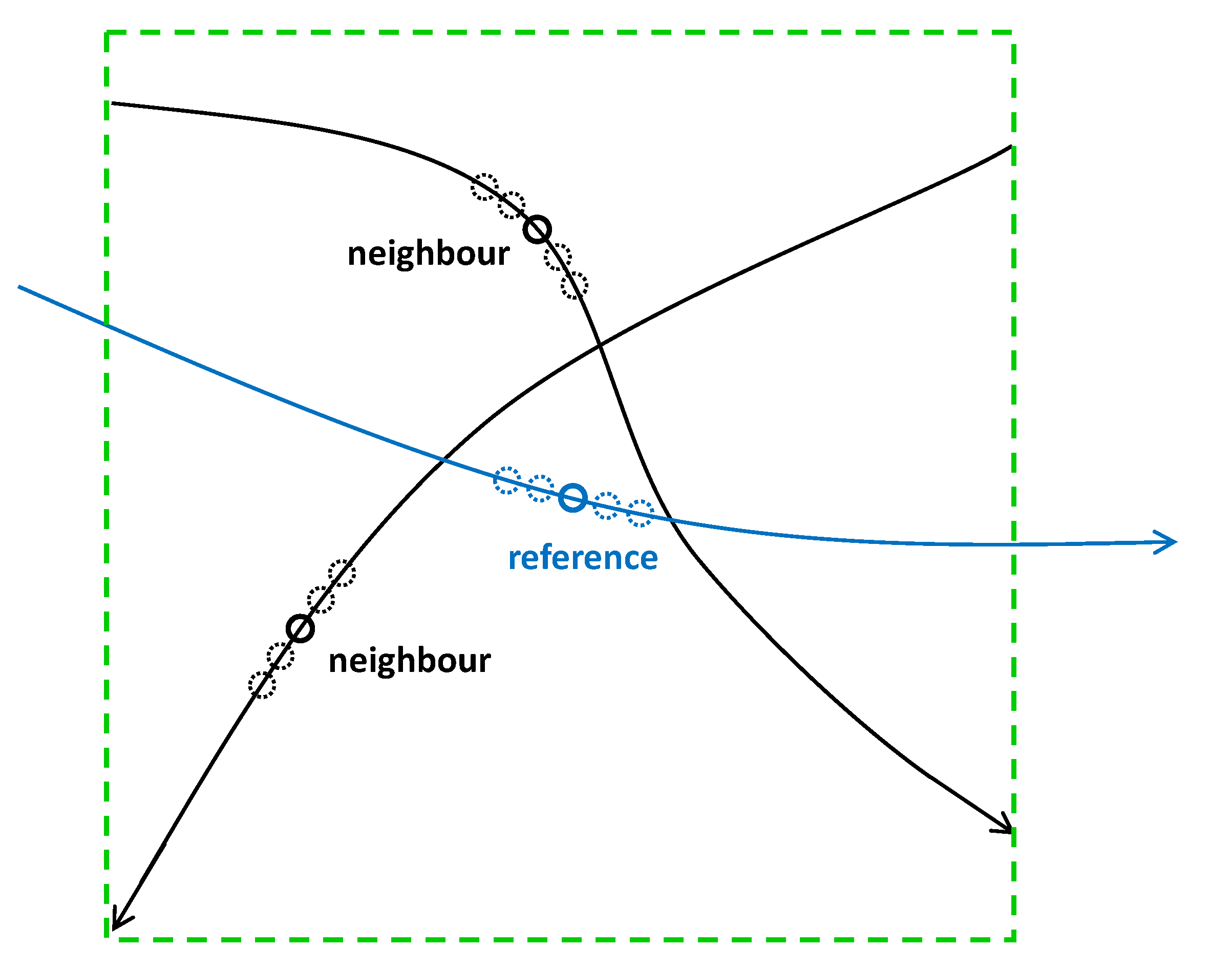
Therefore, the procedure that we apply consists of solving the method while following an aircraft along all the position observations of its trajectory. This aircraft will be referred to as the reference aircraft. As for the aircraft that are flying in its vicinity, they will be referred to as the neighbor aircraft. Every aircraft within the searching area of the reference aircraft at each time will be considered as a neighbor aircraft, and therefore, its observations will be used in the computation (at each time, the neighbor aircraft may be different). This searching area is defined as a box window (24.8 × 24.8 nm) centered at each reference aircraft position. This dimension is based on the longitudinal separation minima applicable to en-route aircraft multiplied by a scalar factor.
The uncertainty extension will be applied to both the reference and neighbor aircraft. Thus, matrix
is computed using the observations of the reference and neighbor aircraft and their uncertainties as well, at each time.
Figure 9 shows the geometry of the problem that is solved for a reference aircraft at a given time.
3.6. Neighborhood Definition
In order to reflect the operational features, the metric has been extended to the third dimension by using a three-dimensional state space. From the operational point of view, what is relevant for air traffic controllers is the horizontal speed of the aircraft and their climbing/descending rate. Thus, the model has been extended in this direction by considering only some aircraft in the neighborhood of a given aircraft.
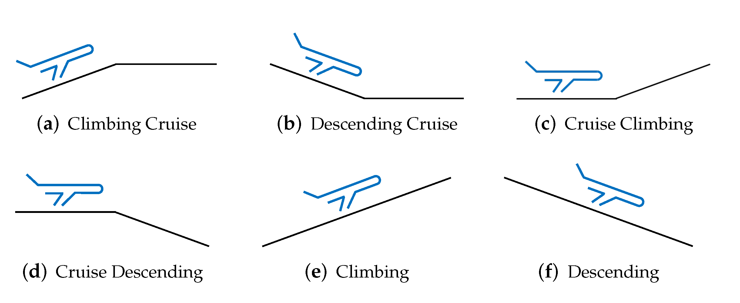
When the reference aircraft is climbing or descending, all the other aircraft in the neighborhood will be considered as neighbors. For a cruising reference aircraft, one must apply filtering to account for aircraft that are flying in the same flight level; however, an extension of this filter was necessary to account for the aircraft that were changing their altitude and then were likely to interact with other aircraft, as they would be flying at the same altitude at some point of the analysis period. The criteria applied to both the reference and neighbor aircraft to filter the possible aircraft affecting the local disorder can be observed in
Figure 10.
When the neighbor aircraft altitude (after applying the searching area principle) is close to the reference aircraft altitude, that neighbor aircraft is considered as an actual neighbor aircraft. In the (Reduced Vertical Separation Minima) airspace, the en-route aircraft vertical separation is 1000 ft between FL290 and FL410. The filter is set to look for neighbor aircraft within a vertical separation, with respect to the reference aircraft altitude, equal to 3000 ft. Therefore, aircraft flying within 30 flight levels above and below the reference aircraft will be considered for the metric. The filter allows the following situations for both the reference and neighbor aircraft: aircraft is climbing to the reference aircraft altitude, aircraft is descending to reference aircraft altitude, aircraft is about to climb from reference aircraft altitude, aircraft is about to descend from reference aircraft altitude, aircraft is climbing and will fly from a lower to a higher altitude than reference aircraft altitude, aircraft is at reference aircraft altitude and aircraft is descending and will fly from a higher to a lower altitude than the reference aircraft altitude.
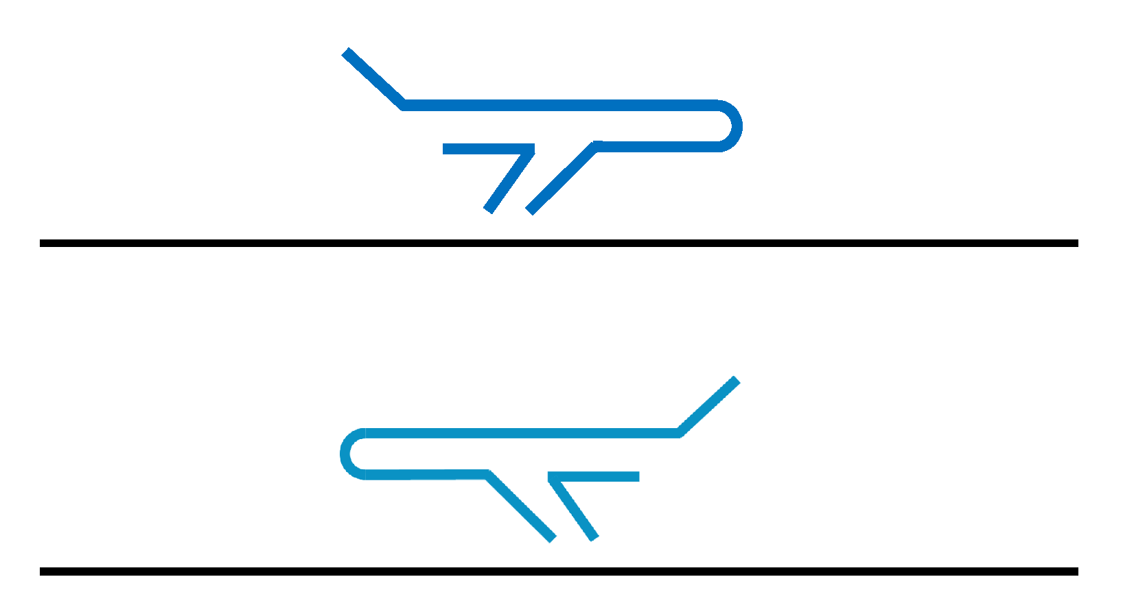
When two cruising aircraft are flying at different altitudes (see the example given in
Figure 11), such aircraft will never be considered as neighbors because they will always stay separated thanks to the vertical separation.
After filtering the neighboring aircraft associated with a reference aircraft (at a given time t), the LMS computation is applied in order to identify the matrix. The metric is then computed based on the eigenvalues of such an matrix and assigned to the reference aircraft at time t. This computation is performed for each trajectory sample along the route.
Having this complexity metric computed along the trajectory, it is possible to establish a color map that exhibits the aircraft involved in congested areas.
4. Results
4.1. Toy Examples
Different traffic samples have been created in order to compare the complexity metric previously described. For the following toy examples, no uncertainties are considered and every aircraft is flying at the same flight level. Six traffic situations will be classed according to an increasing level of difficulty (increasing order of complexity) as a function of predictability and interdependency between trajectories. The full trajectories of aircraft are shown in the following figures, where a green circle symbolizes their initial positions.
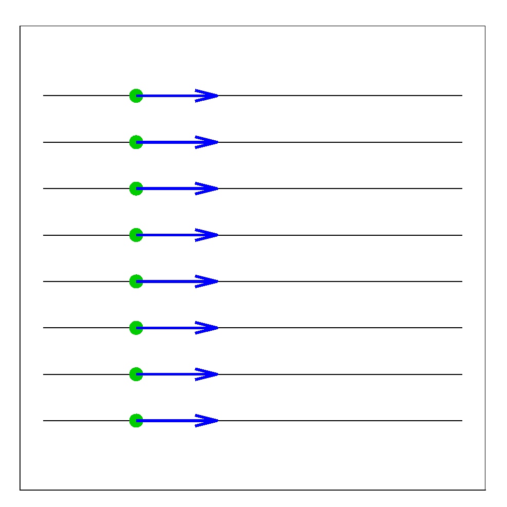
Figure 12 shows a parallel flow of aircraft. It represents an easy situation, where aircraft relative distances stay the same. This situation has no complexity (null
matrix; see Equation (7)).
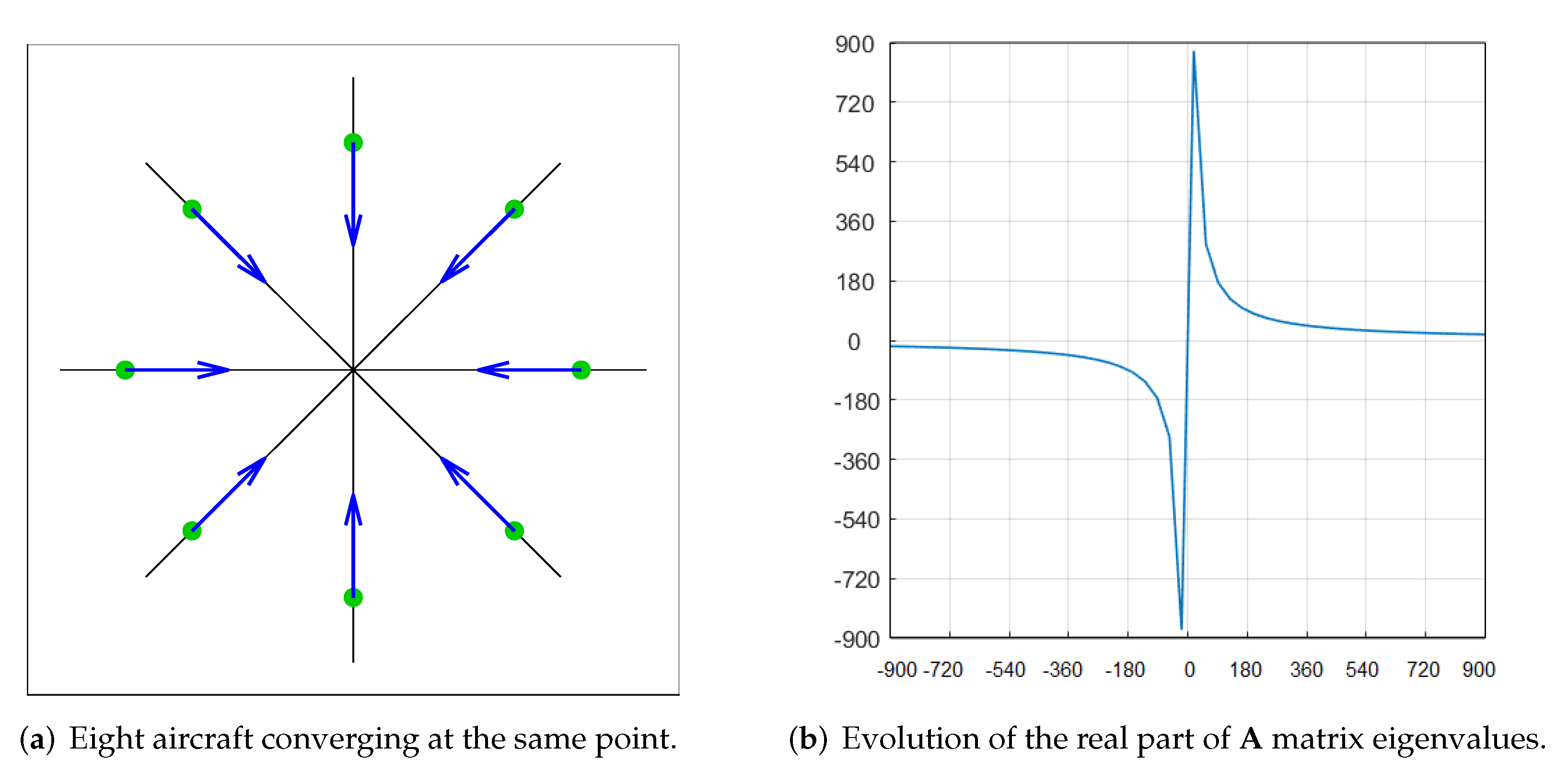
Figure 13a shows a full symmetric convergence of eight aircraft flying at the same speed. It represents an average situation with high sensitivity and conflicts with no interaction between solutions. In order to build an aggregated metric along the time dimension, we compute for each time sample the associated eigenvalues of the
matrix, for which the real parts are summed up in order to produce a scalar value (
Figure 13b). It must be noticed that the metric begins to be negative, demonstrating that the situation is globally converging. Suppose we continue evaluating that situation over time. After the crossing of the aircraft, the metric becomes positive, and the situation is globally diverging.
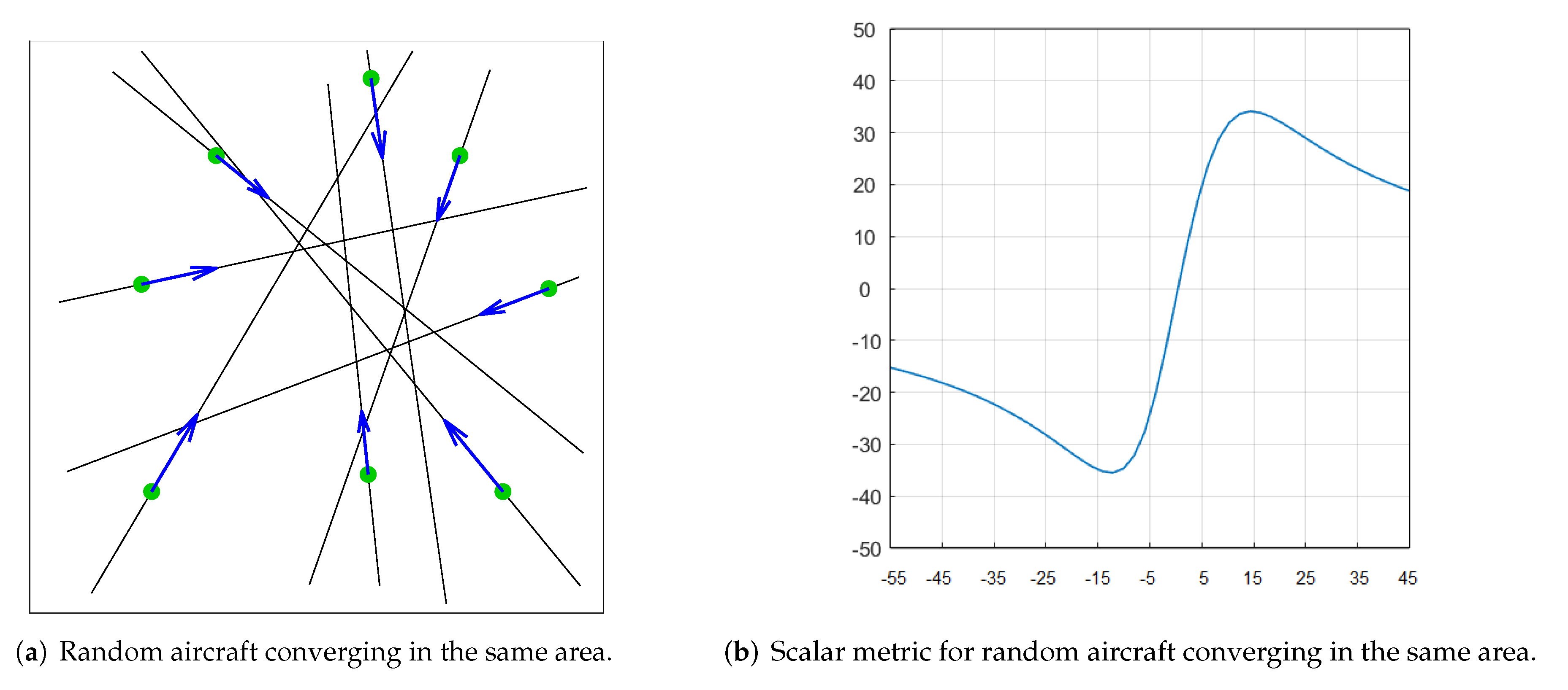
Figure 14a shows a fuzzy convergence of aircraft in the same area. Aircraft do not necessarily have the same speed.
In this case, the metric first identifies a soft converging pattern. Then, it reaches a minimum in the central area of convergence (matching the maximum convergence tendency) and begins to be positive, meaning that the aircraft are diverging at that moment (see
Figure 14b) and then reaches its maximum (matching the maximum divergence tendency).
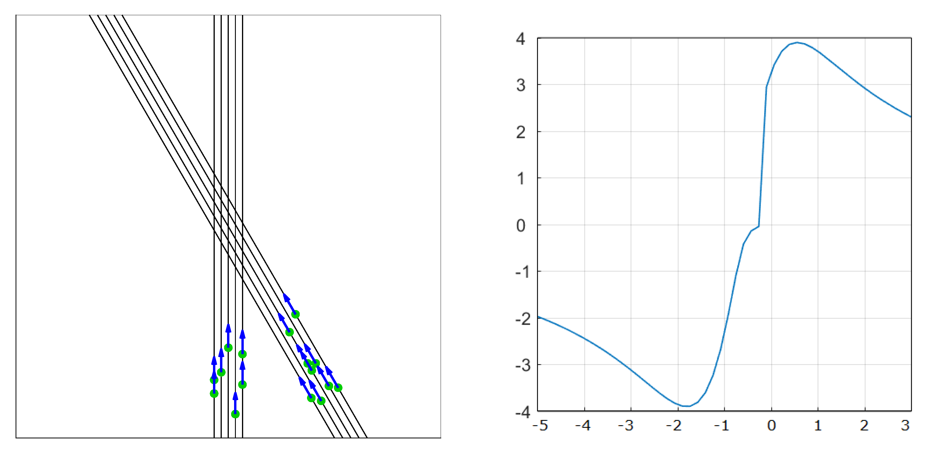
We then consider two flow crossing situations. The first situation has a crossing angle of 30 degrees (see
Figure 15), and the second one has a crossing angle of 90 degrees (see
Figure 16). The right side of both figures represents the evolution of the complexity metric with time. As expected, the metric stat is to be negative as the aircraft start first to converge and become positive (divergence) after the crossing point. The shapes of the curve are the same. Only the magnitude is higher with the 90 deg situation, which is expected, as the relative speed between aircraft is higher in this situation.
It is worth mentioning that in these two cases, each aircraft possesses a different speed. The eigenvalues are always real: the no-curl tendency is perceived, as the set of aircraft are flying only along two different trajectory directions.
4.2. Real Airspace
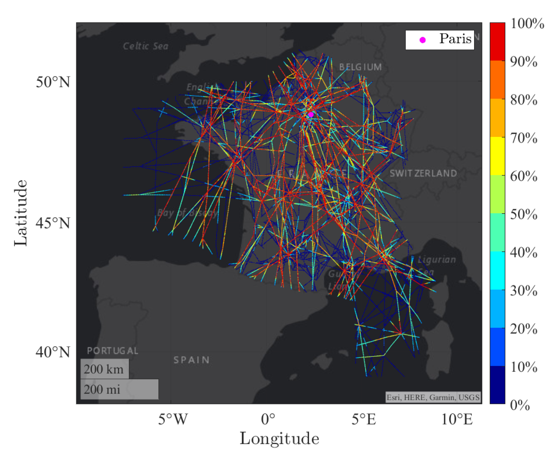
This complexity metric has been computed on traffic simulated with real flight plans of aircraft crossing the French airspace (as a matter of fact, using real traffic data, such as radar tracking records, is meaningless because such traffic has been managed by the controller and complexity has been removed). Based on such flight plans, an arithmetic simulator based on the BADA database has been used in order to create 8000 four-dimensional trajectories in the French airspace. The trajectory has then been sampled every 20 s, representing two million 4D points for the whole day. The metric has been computed for each trajectory and for each time step in a 4D cube (three spatial dimensions and one time dimension) and projected on a two-dimensional coordinate system to have a complexity map, as shown in
Figure 17. On this figure, the metric has been normalized between 0 (blue color) and 100% (maximum with red color). As expected, the highest complexity is located near the big crossings. One must remember that the map represents the accumulated complexity in altitude and time. A 2D point at (x,y) on the map represents all 4D points at those 2D coordinates (x,y).
The metric has been implemented in Java. Thanks to some algorithmic improvements, the computation time needed to compute the metric for the whole day of traffic (two million points) is less than ten milliseconds on a core i7 Laptop computer.
5. Conclusions
This paper has introduced an efficient traffic complexity metric that can identify the level of disorder of a given traffic situation. A Linear Dynamical System model is first regressed based on a least mean square approach, which is based on a set of trajectory samples. An SVD trick has been used in order to avoid conditioning issues in the LMS process. Then, the eigenvalues of the associated matrix of the linear dynamical system are extracted to quantify the disorder of the traffic situation (sum of the negative real parts). When such a metric has to be computed for a predicted traffic situation, one must be able to take into account uncertainties. This uncertainty has been taken into account by considering aircraft as segments in the time dimension in order to produce a robust metric. This metric has been successfully tested on several artificial traffic situations and on a full day of traffic over the French airspace. Based on the high performance for computing this metric (for a large number of trajectories), the next step consists of using this metric in an optimization algorithm to minimize congestion in a given airspace, which is one of the objectives of the START SESAR project.
Author Contributions
Conceptualization, D.D., A.G., S.C. and M.S.; methodology, D.D., A.G., J.L., S.C. and M.S.; software, D.D., A.G. and J.L.; validation, D.D., A.G., J.L., S.C. and M.S. All authors have read and agreed to the published version of the manuscript.
Funding
The SESAR START project has funded the research (grant number 893204).
Institutional Review Board Statement
Not applicable.
Informed Consent Statement
Not applicable.
Data Availability Statement
Not applicable.
Conflicts of Interest
The authors declare no conflict of interest.
Abbreviations
The following abbreviations are used in this manuscript:
| ATC | Air Traffic Control |
| ATM | Air Traffic Management |
| BADA | Base of Aircraft DAta |
| COVID-19 | COrona VIrus Disease-2019 |
| FIR | Flight Information Region |
| LMS | Least Mean Square |
| NASA | National Aeronautics and Space Administration |
| NM | Nautical Mile |
| RVSM | Reduced Vertical Separation Minima |
| SESAR | Single European Sky’s ATM Research |
| START | Stable and resilienT ATM by integrAting Robust airline operations into the neTwork |
| SVD | Singular Value Decomposition |
References
- Sergeeva, M.; Delahaye, D.; Mancel, C.; Vidosavljevic, A. Dynamic airspace configuration by genetic algorithm. J. Traffic Transp. Eng. 2017, 4, 300–314. [Google Scholar] [CrossRef]
- Oussedik, S.; Delahaye, D. Reduction of air traffic congestion by genetic algorithms. Lect. Notes Comput. Sci. 1998, 1498, 855–864. [Google Scholar] [CrossRef] [Green Version]
- Alam, S.; Chaimatanan, S.; Delahaye, D.; Féron, E. A Meta-Heuristic Approach for Distributed Trajectory Planning for European Functional Airspace Blocks. J. Air Transp. 2018, 26, 81–93. [Google Scholar] [CrossRef]
- Wyndemere. An Evaluation of Air Traffic Control Complexity; Technical Report, NASA 2-14284; NASA: Boulder, CO, USA, 1996.
- Laudeman, I.; Shelden, S.; Branstrom, R.; Brasil, C. Dynamic Density: An Air Traffic Management Metric; Technical Report, NASA/TM-1998-112226; NASA: Boulder, CO, USA, 1 April 1998.
- Sridhar, B.; Sheth, K.; Grabbe, S. Airspace complexity and its application in air traffic management. In Proceedings of the 2nd USA/Europe Air Traffic Management R&D Seminar, Orlando, FL, USA, 1–4 December 1998. [Google Scholar]
- Kirwan, B.; Scaife, R.; Kennedy, R. Investigating complexity factors in UK Air Traffic Management. Hum. Factors Aerosp. Saf. 2001, 1, 125–144. [Google Scholar]
- Histon, J.; Hansman, R.; Aigoin, G.; Delahaye, D.; Puechmorel, S. Introducing structural consideration into complexity metrics. In Proceedings of the 4th USA/Europe Air Traffic Management R&D Seminar, Santa Fe, NM, USA, 4–7 December 2001. [Google Scholar]
- Histon, J.; Hansman, R.; Gottlieb, B.; Kleinwaks, H.; Yenson, S.; Delahaye, D.; Puechmorel, S. Structural consideration and cognitive complexity in air traffic control. In Proceedings of the 21st Air Traffic Management for Commercial and Military Systems, Irvine, CA, USA, 27–31 October 2002. [Google Scholar]
- Delahaye, D.; Puechmorel, S. Air traffic complexity: Towards intrinsic metrics. In Proceedings of the 3rd USA/Europe Air Traffic Management R&D Seminar, Napoli, Italy, 13–16 June 2000. [Google Scholar]
- Aigoin, G. Air Traffic Complexity Modeling. Master’s Thesis, Ecole Nationale de l’Aviation Civile, Toulouse, France, 2001. [Google Scholar]
- Mondoloni, S.; Liang, D. Airspace fractal dimension and applications. In Proceedings of the 4th USA/Europe Air Traffic Management R&D Seminar, Santa Fe, NM, USA, 4–7 December 2001. [Google Scholar]
- Delahaye, D.; Paimblanc, P.; Puechmorel, S.; Histon, J.; Hansman, R. A new air traffic complexity metric based on dynamical system modelization. In Proceedings of the 21st Air Traffic Management for Commercial and Military Systems, Irvine, CA, USA, 27–31 October 2002. [Google Scholar]
- Björck, Å. Numerical Methods for Least Squares Problems; Society for Industrial & Applied Mathematics: Philadelphia, PA, USA, 1996. [Google Scholar]
Figure 1.
Radar captures associated with three aircraft. In this example only one time sample is considered.
Figure 1.
Radar captures associated with three aircraft. In this example only one time sample is considered.
Figure 2.
Vector field produced by the linear dynamic system.
Figure 2.
Vector field produced by the linear dynamic system.
Figure 3.
Impact of the eigenvalues of matrix on the dynamics of the system.
Figure 3.
Impact of the eigenvalues of matrix on the dynamics of the system.
Figure 4.
Eigenvalues loci for 4 traffic situations.
Figure 4.
Eigenvalues loci for 4 traffic situations.
Figure 5.
Vector field computed for the 4 toy examples. The red arrows represent the vector field of the associated linear dynamical system model.
Figure 5.
Vector field computed for the 4 toy examples. The red arrows represent the vector field of the associated linear dynamical system model.
Figure 6.
Uncertainties associated with three aircraft.
Figure 6.
Uncertainties associated with three aircraft.
Figure 7.
Vector field of the uncertainties extension.
Figure 7.
Vector field of the uncertainties extension.
Figure 8.
Traffic configuration with and without uncertainties.
Figure 8.
Traffic configuration with and without uncertainties.
Figure 9.
Example of local trajectory interaction at a given time.
Figure 9.
Example of local trajectory interaction at a given time.
Figure 10.
Aircraft altitude evolution that has an interaction with a certain FL.
Figure 10.
Aircraft altitude evolution that has an interaction with a certain FL.
Figure 11.
Lack of interdependency between two consecutive flight level trajectories.
Figure 11.
Lack of interdependency between two consecutive flight level trajectories.
Figure 12.
Parallel flow.
Figure 12.
Parallel flow.
Figure 13.
Scalar metric function of time for eight aircraft converging at the same point. As it is shown, there is a discontinuity when aircraft cross each other but if we consider more aircraft in the crossing, the curve will be scaled accordingly (more aircraft will induce larger negative and positive values).
Figure 14.
Complexity evolution with time associated to the fuzzy convergence situation.
Figure 14.
Complexity evolution with time associated to the fuzzy convergence situation.
Figure 15.
S-N and E-W flows, crossing at 30°. Traffic situation on the left and complexity function of time on the right.
Figure 15.
S-N and E-W flows, crossing at 30°. Traffic situation on the left and complexity function of time on the right.
Figure 16.
S-N and E-W flows, crossing at 90°. Traffic situation on the left and complexity function of time on the right.
Figure 16.
S-N and E-W flows, crossing at 90°. Traffic situation on the left and complexity function of time on the right.
Figure 17.
Traffic complexity of a traffic sample over French airspace. For each 4D point (x,y,z,t) of each trajectory, the complexity metric is computed and represented with a color map on a two dimension map (x,y).
Figure 17.
Traffic complexity of a traffic sample over French airspace. For each 4D point (x,y,z,t) of each trajectory, the complexity metric is computed and represented with a color map on a two dimension map (x,y).
| Publisher’s Note: MDPI stays neutral with regard to jurisdictional claims in published maps and institutional affiliations. |
© 2022 by the authors. Licensee MDPI, Basel, Switzerland. This article is an open access article distributed under the terms and conditions of the Creative Commons Attribution (CC BY) license (https://creativecommons.org/licenses/by/4.0/).


 ,
, 


