Geostationary Station-Keeping of Electric-Propulsion Satellite Equipped with Robotic Arms

Abstract

We propose two approaches based on feedforward control and model-predictive control, respectively, to solve the station-keeping problem of an electric-propulsion geostationary Earth orbit (GEO) satellite, whose thrusters are mounted on two robotic arms on its anti-nadir face. This novel configuration enables a wider range of thrust direction, making it possible to regard the thrust direction as control variables. To solve this control problem, we present the quick feedforward controller (QFFC) and the fuel-optimal model predictive controller (FOMPC). The QFFC is developed based on the analysis of GEO dynamics and the thruster configuration. The FOMPC applies an optimization algorithm to solve the nonlinear model predictive control (NLMPC) problem with the initial value given by the QFFC. Numerical simulations suggest that both controllers could achieve stable station-keeping over multiple objective elements with fewer thrusters and fewer maneuvers. The QFFC has higher control accuracy and lower computational requirements than the FOMPC, whereas the FOMPC could significantly save fuel consumption. The robustness assessment and other discussions of the controllers are also presented.

1. Introduction

Geostationary Earth orbit (GEO) satellites have been playing an important role in applications such as communications, Earth environment, navigation, and aircraft control for decades [1]. To help adjacent satellites avoid colliding with each other, the number of satellites that could be deployed safely around a certain longitude is limited [2]. High-accuracy station-keeping control could alleviate this problem by reducing the required minimum distance or enabling formation flying [3].

Station-keeping by using chemical propulsion is a mature technology and has been applied in plenty of missions [4,5], in which the ground-control center generates the control command by measuring the deviation of the satellite. Due to the nature of the chemical propulsion, chemical-propulsion GEO satellites execute station-keeping maneuvers every two weeks conventionally, resulting in a significant decline in the station-keeping accuracy. In order to solve the problems caused by chemical propulsion, the studies on new types of propulsion, especially electric propulsion, can be traced back to the 1950s [6]. Today, the electric-propulsion satellite has been capable of completing various kinds of space missions [7,8,9], making it possible to form an all-electric satellite platform [10]. The superiority of electric propulsion consists in the high specific impulse, which could significantly reduce the fuel consumption over a lifetime of 12–15 years of GEO satellites [11]. In the past 30 years, multiple electric propulsion systems, such as BPT-4000 [12], SPT-100 [13], and PPS-1350 [14], have been successfully deployed in missions, and the Boeing company also introduced their world’s first all-electric satellite design 702SP in 2012 [10]. During this time, researchers have been paying more attention to station-keeping by using electric propulsion. Oleson et al. investigated applying different electric propulsion systems for the north–south station-keeping [15]. Gomes and Prado used a hybrid optimal control approach to minimize the fuel consumption of the north–south station-keeping [16]. Gazzino et al. decomposed the minimum-fuel station-keeping problem into two steps: first, solve the control problem with an indirect method, and then deal with constraints [17]. They later presented further work in which a three-step decomposition method is employed to solve the same problem [18]. They also investigated solving the same problem via linear integer programming [19,20]. De Bruijn et al. linearized the relative element model in the geostationary station-keeping problem and came up with a method for determining station-keeping maneuvers by using convex optimization based on this model [21]. Min et al. discussed the influence of the configuration of electric thrusters on station-keeping and momentum-dumping [22]. Meanwhile, how to improve the autonomy of the on-board control system is also a focus. Guelmen creatively solved this problem by using a closed-loop control law, which requires the satellite’s real-time position and velocity information [23]. Because real-time GNSS determination is not always available for GEO satellites [24] and the output does not enforce constraints, deploying this method in the application would be challenging. Yang and Li studied the autonomous station-keeping control method for GEO satellites and developed the corresponding software [25]. Park et al. also proposed an autonomous station-keeping system based on the real-time determination [26].

In addition to the above studies, as a promising candidate for solving the station-keeping problem of electric-propulsion GEO satellites, the application of the model-predictive control (MPC) in this area has made significant progress in recent years. Being good at coordinating multiple inputs/outputs and handling constraints [27], the MPC is capable of optimizing the station-keeping performance while considering various constraints in the actual application. Walsh et al. studied applying the MPC for station-keeping and momentum management [28,29,30]. In their work, the controller used a prediction model based on the linearization of the orbital and attitude dynamics of GEO satellites to optimize the fuel consumption while enforcing the constraints caused by the thruster configuration. They chose the classical configuration in which four electric thrusters are fixed on the anti-nadir face of the satellite. Their result, given by the annual velocity increment, is $\Delta V_{\mathrm{AN}}=78.67\mathrm{m}/\mathrm{s}$. In another work of their team, Weiss et al. deployed a six-thruster configuration to save fuel consumption [31] and achieved a better result of $\Delta V_{\mathrm{AN}}=59.4\mathrm{m}/\mathrm{s}$. More thrusters means higher costs and lower reliability. Therefore, Caverly et al. proposed a new configuration where four thrusters are mounted on two assemblies, and they obtained $\Delta V_{\mathrm{AN}}=66.8\mathrm{m}/\mathrm{s}$ [32]. Although this result is higher than that in Ref. [28], it is still very competitive because they considered the on–off nature of the thruster. Unlike these three studies, Zou et al. considered the geostationary station-keeping problem with the MPC as an optimization problem based on the orbital elements instead of the position and velocity [33]. In their study, they combined the linearized relative element model proposed in Ref. [20] with the MPC and obtained $\Delta V_{\mathrm{AN}}=72.3\mathrm{m}/\mathrm{s}$.

In this paper, in contrast to the previous studies, we apply a new configuration where thrusters are mounted on two symmetrical robotic arms. This configuration was first proposed by the Airbus company and had been applied in a space mission with the launch of EUTELSAT 172B in June 2017 [34]. They named it the Deployable Thruster Module Assembly (DTMA) and applied it to the Airbus Eurostar E3000 communication satellite platform. More information about this platform can be found in their introduction [35]. This platform includes a versatile system that enables the thruster to point in the optimal direction, benefiting both orbital transfer and station-keeping missions. Although our study is not based on the specific platform of the Airbus Eurostar E3000, we are inspired by the forward-looking idea of introducing robotic arms into the propulsion system. Therefore, in this paper, we discuss how to design a controller that can take advantage of the wider range of the torque-free thrust direction brought by the robotic arm. The detailed configuration applied in this paper will be stated in a later section.

In the previous MPC-related works, the researchers solved the station-keeping problem within a short prediction horizon based on linear dynamics. Then they quantized the optimal solution to enforce the constraints of the propulsion system, which could avoid handling the nonlinear constraints directly. In this way, the thrust direction will not be regarded as control variables in the control system. However, we believe that changing the thrust direction is critical for saving the fuel consumption of station-keeping. This will make the thrust direction subject to the nonlinear constraints caused by the pitch angle and the yaw angle of the thruster. Therefore, we have to deal with the nonlinear model predictive control (NLMPC) problem if introducing the MPC. The general approach to solving this kind of nonlinear optimization problem is to first find an initial value, and then use the optimization algorithm to obtain the solution, which is why we have to develop an open-loop solver first.

Therefore, in our study, we consider the approach to figuring out the station-keeping problem as three steps: first, we develop a state predictor (SP) to provide the prediction of the orbital states of GEO satellites; then based on our analysis of the GEO dynamics and the thruster configuration, we propose the quick feedforward controller (QFFC) as the open-loop solver, which could work out the solution for the current control cycle. Finally, we combine the SP and the QFFC with the NLMPC problem to form the fuel-optimal model predictive controller (FOMPC). The FOMPC applies a simulated annealing (SA) algorithm to find the optimal control solution with the initial value given by the QFFC. The FOMPC achieves less fuel consumption by optimizing the velocity increment of the north–south station-keeping, considering the station-keeping objective and the thruster configuration as constraints. Simulations show that both the QFFC and the FOMPC could achieve stable station-keeping. The QFFC has minor computational requirements and high accuracy for the station-keeping, while the FOMPC could achieve much less fuel consumption.

This paper is organized as follows. First, the electric thruster configuration and the dynamics are stated in Section 2. Next, in Section 3 and Section 4, we introduce the geostationary station-keeping problem and the proposed controllers in this paper. Then, we present several numerical simulations in Section 5 to evaluate the performance and robustness of the controllers. Finally, we draw conclusions in Section 6.

2. Thruster Configuration and Dynamics

In this paper, we assume a GEO communication satellite equipped with robotic arms whose nominal longitude and latitude of the sub-satellite point are ${\lambda }_{\mathrm{T}}$ and $0^{\circ }$, and the main objective of station-keeping is to maintain the longitude and the latitude of the sub-satellite point. The thruster configuration and the nonlinear orbital dynamics we apply in this station-keeping problem will be stated in this section.

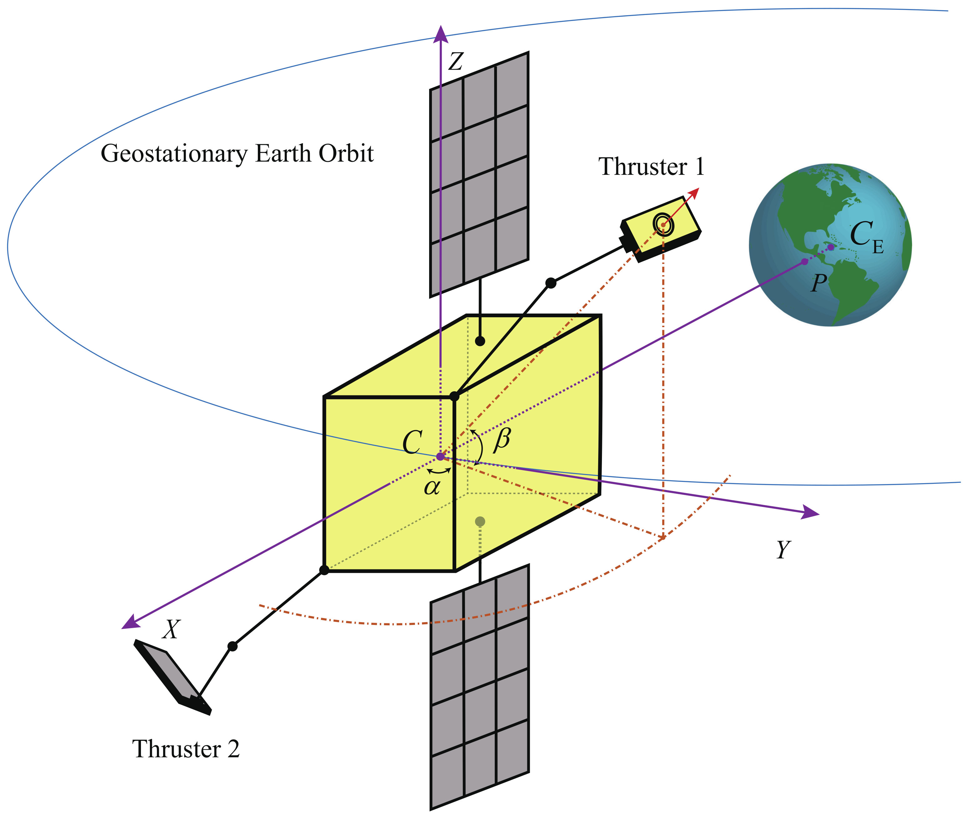
2.1. Thruster Configuration

As we have stated before, the thruster configuration in this paper is characterized by two symmetrical robotic arms placed at the anti-nadir face of the satellite. Thrusters are installed on the platform at the end of two robotic arms, providing the motorization to enable a wider range of thrust direction. Figure 1 shows the model of a GEO satellite that applies this configuration in the RSW (radial, along-track, cross-track) coordinate system, where C and $C_{\mathrm{E}}$ are the centers of mass of the satellite and the Earth, respectively. and P represents the sub-satellite point on the ground, whose longitude and latitude are supposed to be ${\lambda }_{\mathrm{T}}$ and $0^{\circ }$. The X-axis is in the orbital plane and points to the anti-nadir direction, while the Z-axis is perpendicular to the orbital plane. The robotic arms are installed on the two corners of the satellite’s anti-nadir face symmetrically. Due to the requirement of the antenna direction, the attitude of the satellite shown in Figure 1 is fixed during the working of the communication module.

With the help of the robotic arm, the thrusters are capable of flexible motion. The thrust direction in this paper is defined as the torque-free direction that passes through the center of mass of the satellite. Because momentum management is not involved in this paper, we do not consider the inside mechanics of the robotic arm. The thrust direction could be given by the yaw angle $\alpha$ and the pitch angle $\beta$, as shown in Figure 1. $\alpha$ represents the angle between the projection of the thrust direction in the X–Y plane and the +X-axis, while $\beta$ represents the angle between the thrust direction and the X–Y plane. In this paper, we generally assume that thruster 1 could only work within $(+++)$ and $(+-+)$ space, and thruster 2 could only work within $(++-)$ and $(+--)$ space. Thus, we could simplify the range of the feasible thrust direction to several inequality constraints, which could be given by

$$\begin{array}{cc}\hfill -{\alpha }_{min}\le & {\alpha }_1\le {\alpha }_{max}\hfill \\ \hfill -{\alpha }_{max}\le & {\alpha }_2\le {\alpha }_{min}\hfill \\ \hfill {\beta }_{min}\le & {\beta }_1\le {\beta }_{max}\hfill \\ \hfill -{\beta }_{max}\le & {\beta }_2\le -{\beta }_{min}\hfill \end{array}$$

(1)

where ${\alpha }_1$, ${\beta }_1$, ${\alpha }_2$, ${\beta }_2$ are corresponding to thruster 1 and thruster 2, respectively, and ${\alpha }_{max}$, ${\alpha }_{min}$, ${\beta }_{max}$, ${\beta }_{min}$ are nonnegative parameters. We will discuss the impact of these parameters in Section 5.

2.2. Dynamics

The acceleration of the GEO satellite ${\mathbf{a}}_{\mathrm{sat}}$ mainly consists of two parts, which could be written as

$${\mathbf{a}}_{\mathrm{sat}}={\mathbf{a}}_{\mathrm{thr}}+{\mathbf{a}}_{\mathrm{p}}$$

(2)

where ${\mathbf{a}}_{\mathrm{thr}}$ is the acceleration generated by the thruster, and ${\mathbf{a}}_{\mathrm{p}}$ represents the perturbation acceleration.

GEO satellites are mainly affected by the solar and lunar gravitational attraction, the non-spherical perturbation of the Earth, and the solar radiation pressure [36]. Furthermore, the solar and lunar gravitational attraction not only changes the satellite’s inclination, but its components in the orbital plane also have a considerable impact on the semi-major axis and the eccentricity vector, making it the most important item among all perturbations. For the non-spherical perturbation of the Earth, we only consider the $J_2$ perturbation and ignore the remaining higher-order terms. The solar radiation pressure depends on many factors, such as the reflection coefficient and the surface-to-mass ratio of the satellite, and it does not have much influence on the orbital elements compared to the former two perturbations. Nevertheless, the solar radiation pressure is generally considered when studying the geostationary station-keeping problem due to its impact on the attitude of the satellite. Although this paper does not involve momentum management, we take the perturbation of solar radiation pressure into account to be consistent with other studies. Thus, these perturbation accelerations could be expressed as [31]

$${\mathbf{a}}_{\mathrm{p}}={\mathbf{a}}_{\mathrm{sun}}+{\mathbf{a}}_{\mathrm{moon}}+{\mathbf{a}}_{{\mathrm{J}}_2}+{\mathbf{a}}_{\mathrm{srp}}$$

(3)

where ${\mathbf{a}}_{\mathrm{sun}}$, ${\mathbf{a}}_{\mathrm{moon}}$, ${\mathbf{a}}_{{\mathrm{J}}_2}$, and ${\mathbf{a}}_{\mathrm{srp}}$ are the perturbations of the solar and lunar gravitational attraction, the $J_2$ perturbation, and the solar radiation pressure, respectively. Their analytic expressions are [37]

$$\begin{array}{cc}\hfill {\mathbf{a}}_{\mathrm{q}}& ={\mu }_{\mathrm{q}}\left(\frac{{\mathbf{R}}_{\mathrm{q}}}{{\Delta }_{\mathrm{q}}^3}-\frac{{\mathbf{r}}_{\mathrm{q}}}{r_{\mathrm{q}}^3}\right)(\mathrm{q}\mathrm{represents}\mathrm{the}\mathrm{sun}\mathrm{or}\mathrm{the}\mathrm{moon})\hfill \\ \hfill {\mathbf{a}}_{{\mathrm{J}}_2}& =\frac{3\mu J_2{r}_{\mathrm{E}}^2}{2r^5}\left[\left(5\frac{\mathbf{r}·{\widehat{\mathbf{z}}}_{\mathrm{ECI}}}{r^2}-1\right)\mathbf{r}-2\left(\mathbf{r}·{\widehat{\mathbf{z}}}_{\mathrm{ECI}}\right){\widehat{\mathbf{z}}}_{\mathrm{ECI}}\right]\hfill \\ \hfill {\mathbf{a}}_{\mathrm{srp}}& =-{\rho }_{\mathrm{sun}}\left(1+\eta \right)\frac{S_{\mathrm{e}}}{m}\frac{r_{\mathrm{sun}}^2}{{\Delta }_{\mathrm{sun}}^2}{\widehat{\mathbf{R}}}_{\mathrm{sun}}\hfill \end{array}$$

(4)

where $\mu$, ${\mu }_{\mathrm{sun}}$, and ${\mu }_{\mathrm{moon}}$ are the gravitational constants of the Earth, the sun, and the moon, ${\mathbf{R}}_{\mathrm{q}}$ is the position vector of q relative to the satellite, ${\mathbf{r}}_{\mathrm{q}}$ is the position vector of q relative to the Earth, $\mathbf{r}$ is the position vector of the satellite, $J_2$ is a coefficient in the non-spherical perturbation model, ${\widehat{\mathbf{z}}}_{\mathrm{ECI}}$ is the unit vector of the Z-axis in the Earth-centered inertial (ECI) coordinate system, ${\rho }_{\mathrm{sun}}$ is the solar radiation pressure around the Earth, and $\eta$ and $\frac{S_{\mathrm{e}}}{m}$ are the reflection coefficient and the effective surface-to-mass ratio of the satellite. ${\mathbf{a}}_{\mathrm{sat}}$ and all its components are in the ECI coordinate system, which would be more useful if transformed into the RSW coordinate system as ${\left[a_{\mathrm{r}},a_{\mathrm{t}},a_{\mathrm{n}}\right]}^{\mathrm{T}}$.

In order to avoid singularity, we adopt the modified equinoctial elements instead of the Kepler orbital elements in our study. The modified equinoctial elements are given by [38]

$$\begin{array}{cc}\hfill & p=a\left(1-e^2\right)\hfill \\ \hfill & f=ecos\left(\omega +\mathsf{\Omega }\right)\hfill \\ \hfill & g=esin\left(\omega +\mathsf{\Omega }\right)\hfill \\ \hfill & h=tan\left(i/2\right)cos\mathsf{\Omega }\hfill \\ \hfill & k=tan\left(i/2\right)sin\mathsf{\Omega }\hfill \\ \hfill & L=\mathsf{\Omega }+\omega +\theta \hfill \end{array}$$

(5)

in which $\left\{a,e,i,\mathsf{\Omega },\omega \right\}$ belong to the Kepler orbital elements, and $\theta$ is the true anomaly. The high-precision propagation of $\left\{p,f,g,h,k,L\right\}$ is based on the Gauss variational equations [38], which could be written as

$$\begin{array}{cc}\hfill & \dot{p}=\sqrt{\frac{p}{\mu }}\frac{2p}{w}{a}_t\hfill \\ \hfill & \dot{f}=\sqrt{\frac{p}{\mu }}\left\{a_{\mathrm{r}}sinL+\left[\left(1+w\right)cosL+f\right]\frac{a_{\mathrm{t}}}{w}-\left(hsinL-kcosL\right)\frac{g·a_{\mathrm{n}}}{w}\right\}\hfill \\ \hfill & \dot{g}=\sqrt{\frac{p}{\mu }}\left\{-a_{\mathrm{r}}cosL+\left[\left(1+w\right)sinL+g\right]\frac{a_{\mathrm{t}}}{w}+\left(hsinL-kcosL\right)\frac{f·a_{\mathrm{n}}}{w}\right\}\hfill \\ \hfill & \dot{h}=\sqrt{\frac{p}{\mu }}\frac{s^2{a}_{\mathrm{n}}}{2w}cosL\hfill \\ \hfill & \dot{k}=\sqrt{\frac{p}{\mu }}\frac{s^2{a}_{\mathrm{n}}}{2w}sinL\hfill \\ \hfill & \dot{L}=\sqrt{\mu p}{\left(\frac{w}{p}\right)}^2+\frac{1}{w}\sqrt{\frac{p}{\mu }}\left(hsinL-kcosL\right)a_{\mathrm{n}}\hfill \end{array}$$

(6)

where w and $s^2$ are defined as

$$\begin{array}{cc}\hfill & w=1+fcosL+gsinL\hfill \\ \hfill & s^2=1+h^2+k^2.\hfill \end{array}$$

(7)

3. Geostationary Station-Keeping Problem

In this section, we state the objective of geostationary station-keeping first. Then, combined with the thruster configuration mentioned in the previous section, we introduce some constraints into this problem. Finally, we present the control variables of the station-keeping problem and their relationship with the control effect.

3.1. Control Objectives

The primary objective of geostationary station-keeping is to prevent the longitude and the latitude of the GEO satellite from drifting too far. However, in addition to this primary objective, it is also necessary to control the eccentricity vector ${\left[e_x,e_y\right]}^{\mathrm{T}}={[f,g]}^{\mathrm{T}}$, the inclination vector ${\left[i_x,i_y\right]}^{\mathrm{T}}={[h,k]}^{\mathrm{T}}$, and the drift speed of longitude $\dot{\lambda }$, which are important for the stability of station-keeping. Besides, some specific scenarios, such as the multi-satellite collocation, also have requirements for the eccentricity and inclination vectors [3]. Furthermore, due to the perturbations $\lambda$, $e_x$, and $e_y$ have strong short-period oscillations, which makes it inconvenient for us to analyze their deviations. Therefore, we choose the mean elements to describe the orbital state of the GEO satellite, which could be written as

$$\mathbf{x}={\left[\begin{array}{cccccc}\overline{\lambda }& \dot{\overline{\lambda }}& {\overline{e}}_x& {\overline{e}}_y& {\overline{i}}_x& {\overline{i}}_y\end{array}\right]}^{\mathrm{T}}.$$

(8)

The mean elements are obtained by the averaging operator [39]

$$\overline{\epsilon }=\frac{1}{T_{\mathrm{s}}}{\int }_0^{T_{\mathrm{s}}}\epsilon \mathrm{d}t=\frac{1}{2\pi }{\int }_0^{2\pi }\epsilon \mathrm{d}M$$

(9)

where $T_{\mathrm{s}}$ is the orbital cycle of the GEO satellite, and $\overline{\epsilon }$ donates the mean elements in Equation (8). Meanwhile, the objectives of the mean element are given by

$${\mathbf{x}}_{\mathrm{T}}={\left[\begin{array}{cccccc}{\lambda }_{\mathrm{T}}& {\dot{\lambda }}_{\mathrm{T}}& e_{x,\mathrm{T}}& e_{y,\mathrm{T}}& i_{x,\mathrm{T}}& i_{y,\mathrm{T}}\end{array}\right]}^{\mathrm{T}}.$$

(10)

Thus, the deviation $\delta \mathbf{x}$ is

$$\begin{array}{cc}\hfill \delta \mathbf{x}& ={\left[\begin{array}{cccccc}\delta \lambda & \delta \dot{\lambda }& \delta e_x& \delta e_y& \delta i_x& \delta i_y\end{array}\right]}^{\mathrm{T}}\hfill \\ \hfill & ={\left[\begin{array}{cccccc}{\lambda }_{\mathrm{T}}-\overline{\lambda }& {\dot{\lambda }}_{\mathrm{T}}-\dot{\overline{\lambda }}& e_{x,\mathrm{T}}-{\overline{e}}_x& e_{y,\mathrm{T}}-{\overline{e}}_y& i_{x,\mathrm{T}}-{\overline{i}}_x& i_{y,\mathrm{T}}-{\overline{i}}_y\end{array}\right]}^{\mathrm{T}}.\hfill \end{array}$$

(11)

The primary objective of station-keeping is to compensate for $\delta \mathbf{x}$ so as to ensure that $\mathbf{x}={\mathbf{x}}_{\mathrm{T}}$ at the end of each control cycle, thus giving the equality constraints of the station-keeping objective.

3.2. Constraints

In this paper, we consider many constraints while solving the optimization problem instead of enforcing them after obtaining the optimal solution. Some of these constraints are imposed on the satellite, while others are imposed on the station-keeping process. The satellite model equipped with robotic arms that we study in our work is a very specific model. Therefore, we expect that the constraints of the problem could also be close to those in the real application. These constraints could be summarized as follows.

• The thrust direction is limited by the robotic arms, as stated in Section 2.1.
• Although the thrust direction could be adjusted with the robotic arm, the adjustment is supposed to be completed before the maneuver. The robotic arms are locked during the working of thrusters.
• Because station-keeping is carried out at a fixed cycle, the length of each control cycle determines how far the satellite will drift during this time, making it essential to improve the control accuracy. Meanwhile, the control cycle should be the integer multiples of the orbital cycle to simplify the control problem. Therefore, the control cycle is assumed to be one orbital cycle in our work.
• Only one thruster can work at the same time due to the on-board power limitation.
• The reliable ignition times of the thruster are limited. In order to reduce the ignition times, each thruster only ignites once in one control cycle, and each ignition corresponds to one maneuver. For one control cycle, maneuver 1 is performed by thruster 1, and maneuver 2 is performed by thruster 2.
• The only exception to constraint 5 is that the satellite happens to enter the Earth’s shadow while the thruster is still working. Due to the lack of energy, the working of the thruster will be suspended until the satellite leaves the shadow region. In this case, one thruster actually carries out two maneuvers before and after entering the shadow region, but they will be regarded as one maneuver in the optimization.
• To reduce the ignition times, the minimum working time for each maneuver is 30 s.

3.3. Control Solution

Based on the above description, a complete control solution $\mathbf{S}$ for one control cycle should involve eight variables corresponding to the two maneuvers. $\mathbf{S}$ could be written as

$$\mathbf{S}={[{\alpha }_1,{\beta }_1,{\alpha }_2,{\beta }_2,l_1,l_2,V_1,V_2]}^{\mathrm{T}}$$

(12)

where ${\alpha }_1$, ${\alpha }_2$, ${\beta }_1$, and ${\beta }_2$ are the yaw angles and pitch angles of two thrusters, $l_1$ and $l_2$ are the satellite’s right ascensions when conducting the two maneuvers, and $V_1$ and $V_2$ are the velocity increments of the two maneuvers. Because the maneuver usually does not last too long, $l_1$ and $l_2$ could be regarded as the value at the middle, and $V_1$, $V_2$ could be approximate to [40]

$$V_i=\frac{F_{\mathrm{T}}}{m}{D}_i(i=1,2)$$

(13)

in which $F_{\mathrm{T}}$ is the thrust magnitude generated by the thruster, $D_i$ is the length of the i-th maneuver, and m is the mass of the satellite at the beginning of the control cycle, neglecting small mass changes during the maneuver. The relationship between $\mathbf{S}$ and the velocity increments ${\mathbf{v}}_1$, ${\mathbf{v}}_2$ in the RSW coordinate system could be written as

$${\mathbf{v}}_i=\left[\begin{array}{c}{v}_{\mathrm{r}i}\\ v_{\mathrm{t}i}\\ v_{\mathrm{n}i}\end{array}\right]=-V_i\left[\begin{array}{c}cos{\beta }_{i}cos{\alpha }_i\\ cos{\beta }_{i}sin{\alpha }_i\\ sin{\beta }_i\end{array}\right](i=1,2).$$

(14)

The changes of the mean elements caused by the two maneuvers are defined as $\Delta {\mathbf{x}}_1$ and $\Delta {\mathbf{x}}_2$, which are given by

$$\begin{array}{cc}\hfill \Delta {\mathbf{x}}_i& ={\left[\begin{array}{cccccc}\Delta {\lambda }_i& \Delta {\dot{\lambda }}_i& \Delta e_{xi}& \Delta e_{yi}& \Delta i_{xi}& \Delta i_{yi}\end{array}\right]}^{\mathrm{T}}\hfill \\ \hfill & ={\mathbf{B}}_i{\mathbf{v}}_i\hfill \end{array}(i=1,2)$$

(15)

in which ${\mathbf{B}}_i$ is derived from the approximate form of the Gaussian equations [39]

$$\begin{array}{cc}\hfill \dot{a}& =\frac{2R_{\mathrm{s}}}{V_{\mathrm{s}}}{a}_{\mathrm{t}}\hfill \end{array}$$

(16a)

$$\begin{array}{cc}\hfill \dot{\lambda }& =n-{\mathsf{\Omega }}_{\mathrm{E}}-\frac{2}{V_{\mathrm{s}}}{a}_{\mathrm{r}}\hfill \end{array}$$

(16b)

$$\begin{array}{cc}\hfill {\dot{e}}_x& =\frac{1}{V_{\mathrm{s}}}\left(a_{\mathrm{r}}sinl+2a_{\mathrm{t}}cosl\right)\hfill \end{array}$$

(16c)

$$\begin{array}{cc}\hfill {\dot{e}}_y& =\frac{1}{V_{\mathrm{s}}}\left(-a_{\mathrm{r}}cosl+2a_{\mathrm{t}}sinl\right)\hfill \end{array}$$

(16d)

$$\begin{array}{cc}\hfill {\dot{i}}_x& =\frac{cosl}{V_{\mathrm{s}}}{a}_{\mathrm{n}}\hfill \end{array}$$

(16e)

$$\begin{array}{cc}\hfill {\dot{i}}_y& =\frac{sinl}{V_{\mathrm{s}}}{a}_{\mathrm{n}}\hfill \end{array}$$

(16f)

where $R_{\mathrm{s}}$ and $V_{\mathrm{s}}$ are the nominal radius and velocity of GEO satellites, $n=\sqrt{\frac{\mu }{a^3}}$ and $l=\mathsf{\Omega }+\omega +\theta$ are the mean angular velocity and the right ascension, and ${\mathsf{\Omega }}_{\mathrm{E}}$ is the angular rotation rate of the Earth. It could be derived from Equation (16b) that

$$\Delta {\lambda }_i=-\frac{2}{V_{\mathrm{s}}}{v}_{\mathrm{r}i}+\Delta n_i·T_i$$

(17)

$$\Delta {\dot{\lambda }}_i=\Delta n_i$$

(18)

where $\Delta n_i$ is the change of n caused by the i-th maneuver, which is given by

$$\Delta n_i=\frac{\mathrm{d}n}{\mathrm{d}a}·\Delta a_i=-\frac{3}{2}\sqrt{\frac{\mu }{a^5}}·\frac{2R_{\mathrm{s}}}{V_{\mathrm{s}}}{v}_{\mathrm{t}}\approx -\frac{3}{R_{\mathrm{s}}}{v}_{\mathrm{t}}$$

(19)

and $T_{\mathrm{i}}$ is the remaining time of the current control cycle after the i-th maneuver. $T_{\mathrm{i}}$ could be approximate to

$$T_i\approx c_i{T}_{\mathrm{s}}.$$

(20)

The parameter $c_i$ is given by

$$c_i=\left\{\begin{array}{lll}\hfill & 1-\frac{\left(l_i-l_{\mathrm{start}}\right)}{2\pi },\hfill & \hfill \left(l_i\ge l_{\mathrm{start}}\right)\\ \hfill & \frac{\left(l_{\mathrm{start}}-l_i\right)}{2\pi },\hfill & \hfill \left(l_i<l_{\mathrm{start}}\right)\end{array}\right.,0\le l_i,l_{\mathrm{start}}<2\pi$$

(21)

in which $l_{\mathrm{start}}$ is the satellite’s right ascension when the current control cycle starts. In conclusion, ${\mathbf{B}}_i$ could be written as

$${\mathbf{B}}_i=\left[\begin{array}{ccc}-\frac{2}{V_{\mathrm{s}}}& -\frac{3c_i}{V_{\mathrm{s}}}& 0\\ 0& -\frac{3}{R_{\mathrm{s}}}& 0\\ \frac{sin{l}_i}{V_{\mathrm{s}}}& \frac{2cos{l}_i}{V_{\mathrm{s}}}& 0\\ -\frac{cos{l}_i}{V_{\mathrm{s}}}& \frac{2sin{l}_i}{V_{\mathrm{s}}}& 0\\ 0& 0& \frac{cos{l}_i}{2V_{\mathrm{s}}}\\ 0& 0& \frac{sin{l}_i}{2V_{\mathrm{s}}}=\end{array}\right].$$

(22)

Hence, defining the changes of mean elements caused by maneuvers in one control cycle as the control effect $\Delta {\mathbf{x}}_{\mathrm{s}}$, we could establish the relationship between $\mathbf{S}$ and $\Delta {\mathbf{x}}_{\mathrm{s}}$ as

$$\Delta {\mathbf{x}}_{\mathrm{s}}=\Delta {\mathbf{x}}_1+\Delta {\mathbf{x}}_2={\mathbf{B}}_1{\mathbf{v}}_1+{\mathbf{B}}_2{\mathbf{v}}_2=\mathbf{F}\left(\mathbf{S}\right).$$

(23)

4. Station-Keeping Controller Design

In this section, we present the controller design for the geostationary station-keeping problem in this paper, which consists of three parts: the state predictor (SP), the quick feedforward controller (QFFC), and the fuel-optimal model predictive controller (FOMPC).

4.1. State Predictor

Let us define the mean elements at the beginning of the first control cycle as the initial state ${\mathbf{x}}_0$ and the prediction at the end of the k-th control cycle as ${\mathbf{x}}_k$. This can be written as

$${\mathbf{x}}_k={\left[\begin{array}{cccccc}{\overline{\lambda }}_k& {\dot{\overline{\lambda }}}_k& {\overline{e}}_{x,k}& {\overline{e}}_{y,k}& {\overline{i}}_{x,k}& {\overline{i}}_{y,k}\end{array}\right]}^{\mathrm{T}}(k=0,1,2,...).$$

(24)

The primary function of the SP is to obtain the prediction ${\mathbf{x}}_k$, given the initial state ${\mathbf{x}}_0$ and the control solutions of former control cycles $\left\{{\mathbf{S}}_1,{\mathbf{S}}_2,...,{\mathbf{S}}_k\right\}$.

Generally, the element changes caused by station-keeping maneuvers and natural drifts are small within several control cycles, making them independent of each other. Thus, the ${\mathbf{x}}_k$ can be obtained by

$${\mathbf{x}}_k={\mathbf{x}}_{k-1}+\Delta {\mathbf{x}}_{\mathrm{s},k}+\Delta {\mathbf{x}}_{\mathrm{d},k}$$

(25)

in which $\Delta {\mathbf{x}}_{\mathrm{s},k}$ and $\Delta {\mathbf{x}}_{\mathrm{d},k}$ are the element changes caused by maneuvers and natural drifts, respectively. $\Delta {\mathbf{x}}_{\mathrm{s},k}$ can be obtained through Equation (23), while $\Delta {\mathbf{x}}_{\mathrm{d},k}$ can be written as

$$\Delta {\mathbf{x}}_{\mathrm{d},k}={\left[\begin{array}{cccccc}\Delta {\lambda }_{\mathrm{d},k}& \Delta {\dot{\lambda }}_{\mathrm{d},k}& \Delta e_{x\mathrm{d},k}& \Delta e_{y\mathrm{d},k}& \Delta i_{x\mathrm{d},k}& \Delta i_{y\mathrm{d},k}\end{array}\right]}^{\mathrm{T}}.$$

(26)

$\Delta {\mathbf{x}}_{\mathrm{d},k}$ could be easily obtained in advance through the high-precision orbit propagation. The high-precision orbit propagation is completed in the preparation of the SP and only needs to be conducted once, causing a minor computational burden. Besides, $\Delta {\lambda }_{\mathrm{d},k}$ could be approximate to

$$\Delta {\lambda }_{\mathrm{d},k}\approx {\dot{\overline{\lambda }}}_{k-1}{T}_{\mathrm{s}}.$$

(27)

4.2. Quick Feedforward Controller

With the help of the SP, we present the quick feedforward controller (QFFC). The primary function of the QFFC is to quickly work out the control solution for the current control cycle based on the prediction given by the SP. Because the control objective is to compensate for the deviation of the element, it is required that ${\mathbf{x}}_k={\mathbf{x}}_{\mathrm{T}}$. Therefore, according to Equation (25), the effect of the control solution is supposed to fulfill

$$\Delta {\mathbf{x}}_{\mathrm{s},k}={\mathbf{x}}_{\mathrm{T}}-{\mathbf{x}}_{k-1}-\Delta {\mathbf{x}}_{\mathrm{d},k}.$$

(28)

Defining $\delta {\mathbf{x}}_k={\mathbf{x}}_{\mathrm{T}}-{\mathbf{x}}_{k-1}-\Delta {\mathbf{x}}_{\mathrm{d},k}$ as the predictive deviation of the k-th control cycle, we can obtain the basic rule of the feedforward control as

$$\delta {\mathbf{x}}_k=\Delta {\mathbf{x}}_{\mathrm{s},k}={\mathbf{B}}_{1,k}{\mathbf{v}}_{1,k}+{\mathbf{B}}_{2,k}{\mathbf{v}}_{2,k}=\mathbf{F}\left({\mathbf{S}}_{\mathbf{k}}\right)$$

(29)

in which ${\mathbf{B}}_{1,k}$, ${\mathbf{B}}_{2,k}$, ${\mathbf{v}}_{1,k}$, and ${\mathbf{v}}_{2,k}$ are given by Equations (14) and (22).

For ${\mathbf{S}}_k={[{\alpha }_{1,k},{\beta }_{1,k},{\alpha }_{2,k},{\beta }_{2,k},l_{1,k},l_{2,k},V_{1,k},V_{2,k}]}^{\mathrm{T}}$, we make an important simplification first. The last two rows of Equation (29) can be written as

$$\left[\begin{array}{c}\delta i_{x,k}\\ \delta i_{y,k}\end{array}\right]=\frac{v_{\mathrm{n}1,k}}{2V_{\mathrm{s}}}\left[\begin{array}{c}cos{l}_{1k}\\ sin{l}_{1k}\end{array}\right]+\frac{v_{\mathrm{n}2,\mathrm{k}}}{2V_{\mathrm{s}}}\left[\begin{array}{c}cos{l}_{2,k}\\ sin{l}_{2,k}\end{array}\right].$$

(30)

Because the north–south station-keeping dominates the required velocity increment, it must be carried out as efficiently as possible to save fuel consumption. According to Equation (30), ${[cos{l}_{1,k},sin{l}_{1,k}]}^{\mathrm{T}}$ and ${[cos{l}_{2,k},sin{l}_{2,k}]}^{\mathrm{T}}$ have to be in the same or opposite direction as $[\delta i_{x,k},\delta i_{y,k}]$ to maximize the efficiency of north–south station-keeping, meaning that either $l_{2,k}=l_{1,k}$ or $l_{2,k}=l_{1,k}+\pi$. If $l_{2,k}=l_{1,k}$, the two maneuvers will be equivalent to one larger maneuver, contrary to our original intention of setting two maneuvers. Therefore, based on $l_{2,k}=l_{1,k}+\pi$, we could obtain that

$$l_{2,k}=l_{1,k}+\pi =arctan\left(\frac{\delta i_{y,k}}{\delta i_{x,k}}\right).$$

(31)

This simplification would reduce the number of variables in the control solution from eight to six.

Then Equation (29) could be rewritten as

$$\begin{array}{cc}\hfill V_{\mathrm{L},k}& =v_{\mathrm{r}1,k}+v_{\mathrm{r}2,k}+\frac{3}{2}(c_{1,k}{v}_{\mathrm{t}1,k}+c_{2,k}{v}_{\mathrm{t}2,k})\hfill \end{array}$$

(32a)

$$\begin{array}{cc}\hfill V_{\mathrm{DT},k}& =v_{\mathrm{t}1,k}+v_{\mathrm{t}2,k}\hfill \end{array}$$

(32b)

$$\begin{array}{cc}\hfill V_{\mathrm{R},k}& =v_{\mathrm{r}1,k}-v_{\mathrm{r}2,k}\hfill \end{array}$$

(32c)

$$\begin{array}{cc}\hfill V_{\mathrm{ET},k}& =v_{\mathrm{t}1,k}-v_{\mathrm{t}2,k}\hfill \end{array}$$

(32d)

$$\begin{array}{cc}\hfill V_{\mathrm{N},k}& =v_{\mathrm{n}1,k}+v_{\mathrm{n}2,k}\hfill \end{array}$$

(32e)

among which $V_{\mathrm{L},k}$, $V_{\mathrm{DT},k}$, $V_{\mathrm{R},k}$, $V_{\mathrm{ET},k}$, $V_{\mathrm{N},k}$ are defined as

$$\begin{array}{cc}\hfill V_{\mathrm{L},k}& =-\frac{V_{\mathrm{s}}}{2}\delta {\lambda }_k\hfill \end{array}$$

(33a)

$$\begin{array}{cc}\hfill V_{\mathrm{DT},k}& =-\frac{R_{\mathrm{s}}}{3}\delta {\dot{\lambda }}_k\hfill \end{array}$$

(33b)

$$\begin{array}{cc}\hfill V_{\mathrm{R},k}& =V_{\mathrm{s}}\left[\delta e_{x,k}sin{l}_{1,k}-\delta e_{y,k}cos{l}_{1,k}\right]\hfill \end{array}$$

(33c)

$$\begin{array}{cc}\hfill V_{\mathrm{ET},k}& =\frac{V_{\mathrm{s}}}{2}\left[\delta e_{x,k}cos{l}_{1,k}+\delta e_{y,k}sin{l}_{1,k}\right]\hfill \end{array}$$

(33d)

$$\begin{array}{cc}\hfill V_{\mathrm{N},k}& =\frac{2V_{\mathrm{s}}}{cos{l}_1}\delta i_{x,k}=\frac{2V_{\mathrm{s}}}{sin{l}_1}\delta i_{y,k}.\hfill \end{array}$$

(33e)

So far, if the control system is not subject to any constraint, it would be easy to obtain the solution by solving Equations (32a)–(32e). It is worth noting that there is usually more than one solution for Equations (32a)–(32e), among which we choose the one that minimizes $V_{1,k}+V_{2,k}$ as the control solution.

Furthermore, because the thruster cannot face the nadir direction as stated in Section 2.1, it is obvious that

$$v_{\mathrm{r}1,k}\le 0,v_{\mathrm{r}2,k}\le 0.$$

(34)

Then by combining Equation (34) with Equations (32a)–(32d), we could obtain

$$V_{\mathrm{L},k}-\frac{3}{4}\left(c_{1,k}+c_{2,k}\right)V_{\mathrm{DT},k}-\frac{3}{4}\left(c_{1,k}-c_{2,k}\right)V_{\mathrm{ET},k}+\left|V_{\mathrm{R},k}\right|\le 0.$$

(35)

Equation (35) is a necessary condition for Equations (32a)–(32e) to have a solution. If the $V_{\mathrm{L},k}$, $V_{\mathrm{DT},k}$, $V_{\mathrm{R},k}$, $V_{\mathrm{ET},k}$ are all determined, this condition may not be matched. To solve this problem, we have to change some of them to make sure the condition of Equation (35) is satisfied. Changing $V_{\mathrm{L},k}$, $V_{\mathrm{R},k}$, $V_{\mathrm{ET},k}$ means changing $\delta {\lambda }_k$, $\delta e_{x,k}$, $\delta e_{y,k}$, which will directly affect the stability of station-keeping, while changing $V_{\mathrm{DT},k}$ (i.e., changing $\delta {\dot{\lambda }}_k$) will not. Therefore, increasing $V_{\mathrm{DT},k}$ until we obtain a solution is the only option under these circumstances.

Although $V_{\mathrm{L},k}$ has been determined for the current control cycle, we can still change $V_{\mathrm{L},k+1}$ indirectly by changing $V_{\mathrm{DT},k}$, making it easier for the condition of Equation (35) to be matched in the next control cycle. The condition of Equation (35) in the next control cycle can be written as

$$\begin{array}{cc}\hfill V_{\mathrm{L},k+1}& \le \frac{3}{4}\left(c_{1,k+1}+c_{2,k+1}\right)V_{\mathrm{DT},k+1}\hfill \\ \hfill & +\frac{3}{4}\left(c_{1,k+1}-c_{2,k+1}\right)V_{\mathrm{ET},k+1}-\left|V_{\mathrm{R},k+1}\right|\hfill \end{array}$$

(36)

in which $V_{\mathrm{ET},k+1}$ and $V_{\mathrm{R},k+1}$ are determined by the prediction of ${\delta \mathbf{x}}_{k+1}$, and $V_{\mathrm{DT},k+1}$ is related to later control cycles. Thus, we assume that $V_{\mathrm{DT},k+1}=0$ and obtain the estimate of the required $V_{\mathrm{L},k+1}$ in the next control cycle as

$${\tilde{V}}_{\mathrm{L},k+1}=\frac{3}{4}\left(c_{1,k+1}-c_{2,k+1}\right)V_{\mathrm{ET},k+1}-\left|V_{\mathrm{R},k+1}\right|.$$

(37)

Because

$${\dot{\overline{\lambda }}}_k\approx \frac{\Delta {\lambda }_{\mathrm{d},k+1}}{T_{\mathrm{s}}}=\frac{{\lambda }_{\mathrm{T}}-{\overline{\lambda }}_k-\delta {\lambda }_{k+1}}{T_{\mathrm{s}}}=-\frac{\delta {\lambda }_{k+1}}{T_{\mathrm{s}}}=\frac{2}{R_{\mathrm{s}}}{\tilde{V}}_{\mathrm{L},k+1},$$

(38)

the estimate of the required $V_{\mathrm{DT},k}$ can be given by

$$\begin{array}{cc}\hfill {\tilde{V}}_{\mathrm{DT},k}& =-\frac{R_{\mathrm{s}}}{3}\delta {\dot{\lambda }}_k=-\frac{R_{\mathrm{s}}}{3}\left({\dot{\overline{\lambda }}}_k-{\dot{\overline{\lambda }}}_{k-1}-\Delta {\dot{\lambda }}_{\mathrm{d},k}\right)\hfill \\ & =-\frac{2}{3}{\tilde{V}}_{\mathrm{L},k+1}+\frac{R_{\mathrm{s}}}{3}\left({\dot{\overline{\lambda }}}_{k-1}+\Delta {\dot{\lambda }}_{\mathrm{d},k}\right).\hfill \end{array}$$

(39)

The intention of this step is not to guarantee the satisfaction of the condition of Equation (35). In fact, it would not help the situation of the current control cycle. If ${\tilde{V}}_{\mathrm{DT},k}$ cannot satisfy the condition of Equation (35), we still need to increase $V_{\mathrm{DT},k}$ based on ${\tilde{V}}_{\mathrm{DT},k}$ until we obtain a solution. Changing $V_{\mathrm{L},k+1}$ indirectly could avoid a large adjustment to $V_{\mathrm{DT},k+1}$ in the next control cycle. On the whole, this will smooth the variation of $\dot{\overline{\lambda }}$, thereby enhancing the stability of the station-keeping and slightly reducing fuel consumption.

In summary, by establishing the relationship between the control solution and the control objective, we design the QFFC based on the feedforward control. The QFFC mainly has two roles: an open-loop solver in the following FOMPC or an autonomous on-board controller. We will evaluate the performance of the QFFC in Section 5.

4.3. Fuel-Optimal Model Predictive Controller

The QFFC stated above obtains the solution by adjusting $V_{\mathrm{DT}}$. Not optimal though the $V_{\mathrm{DT}}$ is, it has little influence on the overall fuel consumption due to its small proportion of the required velocity increment. Actually, the required velocity increment is dominated by north–south station-keeping. Therefore, to effectively optimize the fuel consumption, the controller needs to adjust the $V_{\mathrm{N}}$ of each control cycle according to the prediction given by the SP. On the other hand, the analysis of the condition of Equation (35) is only concerned with the in-plane components of the velocity increment. Under extreme circumstances, the QFFC may not be able to give the solution, which has to be fixed by adjusting $V_{\mathrm{N}}$. Adjusting $V_{\mathrm{N}}$ means we just need to ensure that the deviation of the inclination vector does not exceed the threshold $\Delta i_{max}$ at the end of each control cycle instead of requiring ${\left[{\overline{i}}_x,{\overline{i}}_y\right]}^{\mathrm{T}}={\left[i_{x,\mathrm{T}},i_{y,\mathrm{T}}\right]}^{\mathrm{T}}$ strictly. Defining the value of $V_{\mathrm{N}}$ applied in the k-th control cycle as $u_k$, we could regard the process to obtain the control solution by the QFFC as a function of $u_k$, which can be written as

$${\mathbf{S}}_k=\left\{\begin{array}{ccc}\hfill & {\left.\mathbf{Q}\left(u_k\right)\right|}_{\delta \mathbf{x}=\delta {\mathbf{x}}_k},\hfill & \hfill \mathrm{if}\mathrm{solution}\mathrm{exists}\\ \hfill & \mathbf{0},\hfill & \hfill \mathrm{if}\mathrm{solution}\mathrm{does}\mathrm{not}\mathrm{exist}.\end{array}\right.$$

(40)

Therefore, the nonlinear model predictive control (NLMPC) problem can be formulated as

$$\begin{array}{cc}\hfill \underset{{\mathbf{U}}_h}{min}& \frac{1}{2}\sum _{k=1}^N(V_{1,k|h}^2+V_{2,k|h}^2)\hfill \\ \hfill \mathrm{s}.\mathrm{t}.& {\mathbf{x}}_{k|h}={\mathbf{x}}_{k-1|h}+\Delta {\mathbf{x}}_{\mathrm{s},k|h}+\Delta {\mathbf{x}}_{\mathrm{d},k|h},\hfill \\ \hfill & {\mathbf{x}}_{0|h}={\mathbf{x}}_h,\hfill \\ \hfill & {\overline{\lambda }}_{k|h}={\lambda }_{\mathrm{T}},\hfill \\ \hfill & {\overline{e}}_{x,k|h}=e_{x,\mathrm{T}},\hfill \\ \hfill & {\overline{e}}_{y,k|h}=e_{y,\mathrm{T}},\hfill \\ \hfill & \sqrt{{\left(i_{x,\mathrm{T}}-{\overline{i}}_{x,k|h}\right)}^2+{\left(i_{y,\mathrm{T}}-{\overline{i}}_{y,k|h}\right)}^2}\le \Delta i_{max},\hfill \\ \hfill & -{\alpha }_{min}\le {\alpha }_{1,k|h}\le {\alpha }_{max},\hfill \\ \hfill & -{\alpha }_{max}\le {\alpha }_{2,k|h}\le {\alpha }_{min},\hfill \\ \hfill & {\beta }_{min}\le {\beta }_{1,k|h}\le {\beta }_{max},\hfill \\ \hfill & -{\beta }_{max}\le {\beta }_{2,k|h}\le -{\beta }_{min},\hfill \\ \hfill & V_{1,k|h}\ge 0,\hfill \\ \hfill & V_{2,k|h}\ge 0\hfill \end{array}$$

(41)

where h is the number of the current control cycle, N is the prediction horizon, ${\varsigma }_{k|h}$ denotes the prediction of $\varsigma$ for k control cycles ahead of h, ${\mathbf{U}}_h={\left[u_{1|h},u_{2|h},...,u_{N|h}\right]}^{\mathrm{T}}$ is the sequence of $u_{k|h}$ within the prediction horizon, ${\mathbf{S}}_{k|h}={[{\alpha }_{1,k|h},{\beta }_{1,k|h},{\alpha }_{2,k|h},{\beta }_{2,k|h},V_{1,k|h},V_{2,k|h}]}^{\mathrm{T}}$ are given by Equation (40). The optimal solution of Equation (41) could be written as ${\mathbf{U}}_h^{*}$, among which we only apply $u_{1|h}^{*}$ to the current control cycle h following the rule of the MPC.

The prediction horizon N determines the number of control cycles involved in a single optimization. When $N=1$, Equation (41) becomes a greedy algorithm for minimizing the fuel consumption of the current cycle; when $N=\infty$, the solution of Equation (41) is the actual global optimum of the station-keeping problem. Therefore, increasing N benefits the performance of the controller in theory. Whereas with the growth of the prediction horizon, the SP cannot keep the prediction accuracy, and the computational requirement increases fast as well. Therefore, the optimal value of N exists. We will verify this in the next section.

There are several practical algorithms to solve the nonlinear optimization problem [41], among which we employ a simulated annealing (SA) algorithm in the optimization. The algorithm was first proposed to solve the combinational optimization problem by simulating the solid annealing phenomenon [42]. The SA has good robustness and parallelism, but it also turns out to be sensitive to the initial value. In our case, the SA is used to find the optimal solution sequence ${\mathbf{U}}_h^{*}$. Based on Equation (41), we define the evaluation function as

$$\begin{array}{cc}\hfill & J\left({\mathbf{U}}_{\mathbf{h}}\right) =\frac{1}{2}\sum _{k=1}^N\left\{V_{1,k|h}^2+V_{2,k|h}^2+{\xi }_k\left[\left(i_{x,\mathrm{T}}-{\overline{i}}_{x,k|h}\right){}^2+\left(i_{y,\mathrm{T}}-{\overline{i}}_{y,k|h}\right){}^2\right]\right\},\hfill \\ \hfill & {\xi }_k=\left\{\begin{array}{cc}\hfill & 0,\sqrt{{\left(i_{x,\mathrm{T}}-{\overline{i}}_{x,k|h}\right)}^2+{\left(i_{y,\mathrm{T}}-{\overline{i}}_{y,k|h}\right)}^2}\le \Delta i_{max}\hfill \\ \hfill & P,\sqrt{{\left(i_{x,\mathrm{T}}-{\overline{i}}_{x,k|h}\right)}^2+{\left(i_{y,\mathrm{T}}-{\overline{i}}_{y,k|h}\right)}^2}>\Delta i_{max}\hfill \end{array}\right.\hfill \end{array}$$

(42)

where ${\xi }_k$ and P are penalty parameters to ensure that ${\mathbf{U}}_{\mathbf{h}}$, which fails to enforce the constraint of the inclination vector, has poor performance. The initial value ${\mathbf{U}}_{\mathbf{h}}^0$ of the optimization is given by the QFFC. The algorithm explores the solution space by generating disturbances. In the end, as the temperature continues to drop, and the result of the SA converges to the optimal solution ${\mathbf{U}}_{\mathbf{h}}^{*}$. Applying $u_{1|h}^{*}$ to the current control cycle h, we obtain the fuel-optimal control solution. The performance of the FOMPC will be evaluated in Section 5.

5. Numerical Simulations

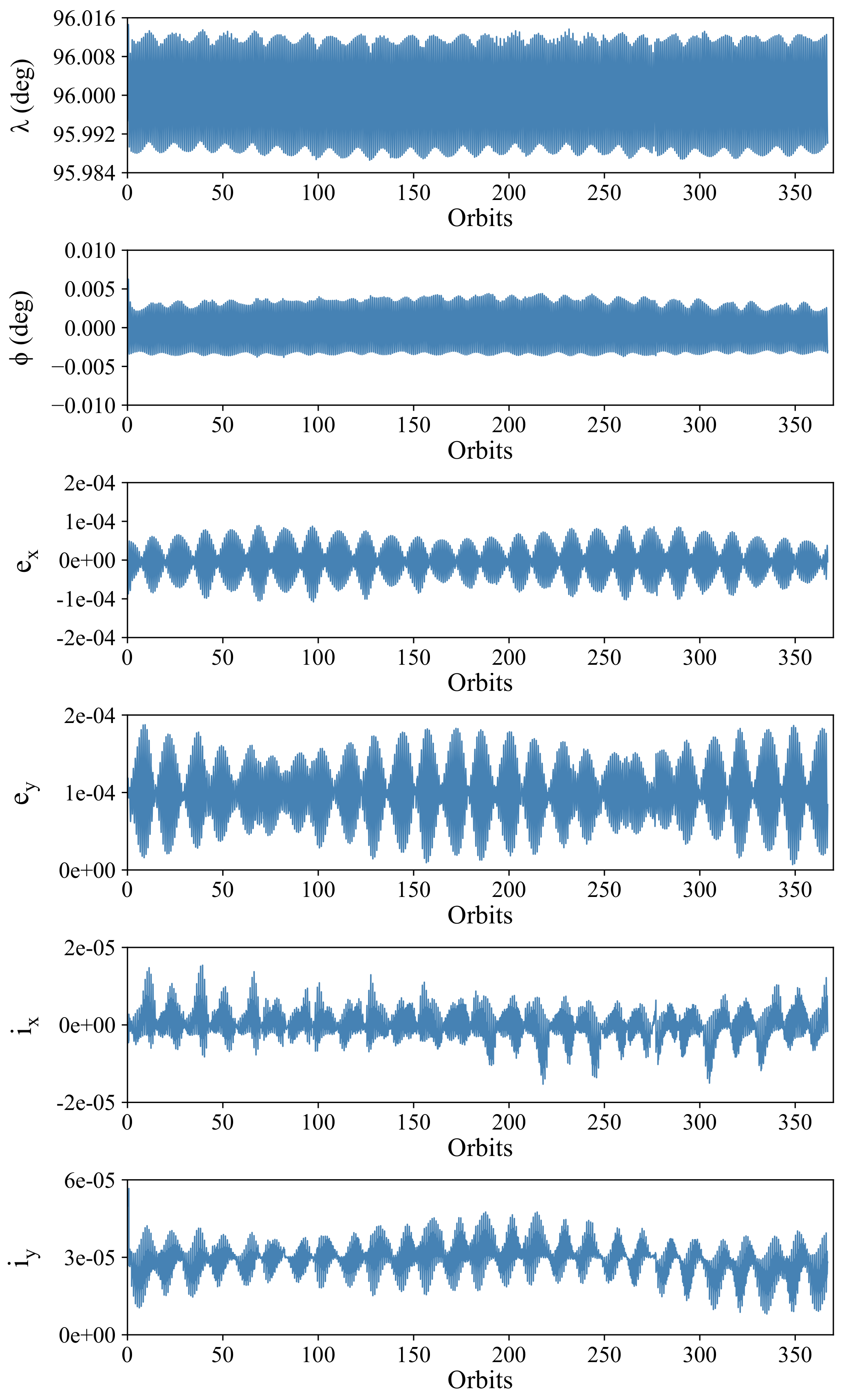
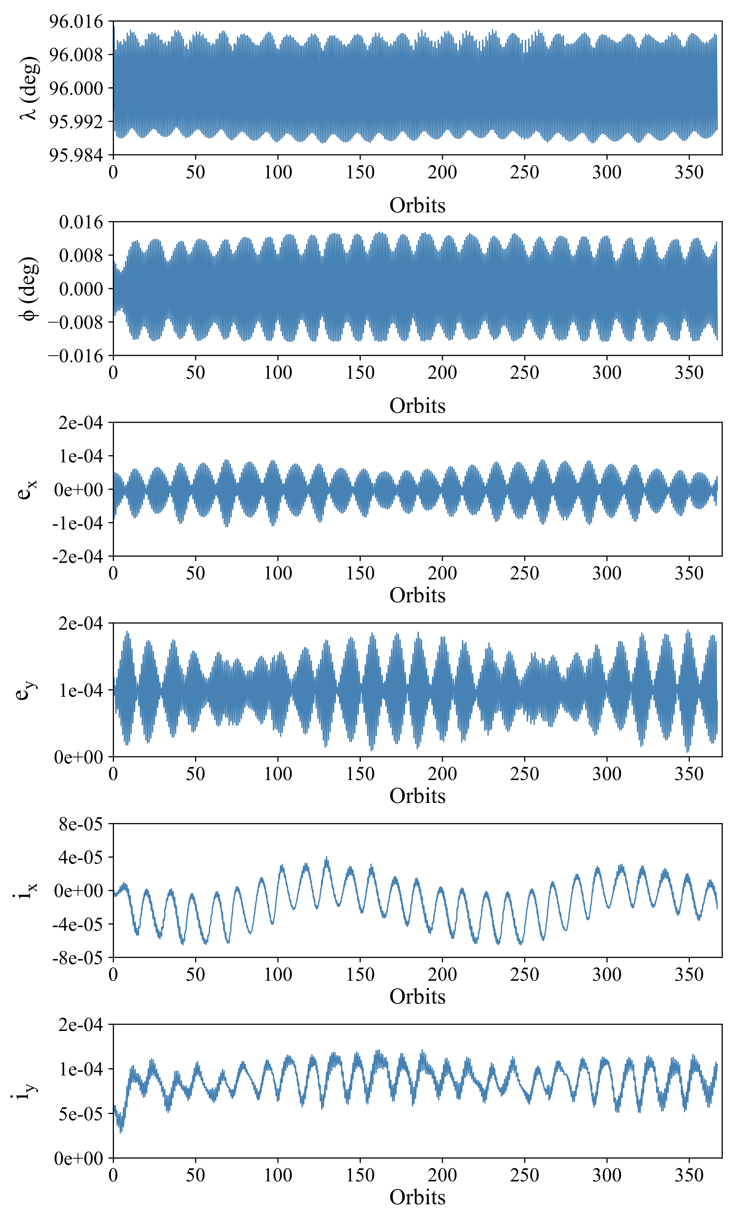
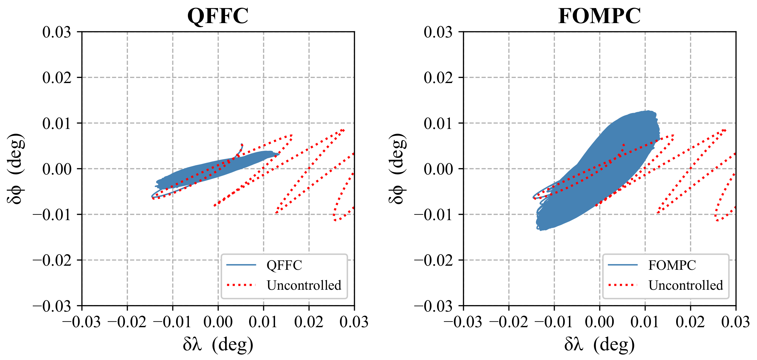
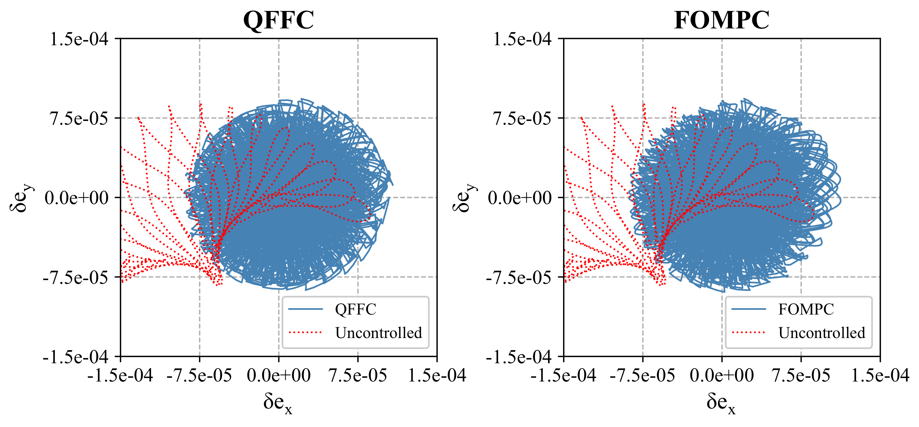
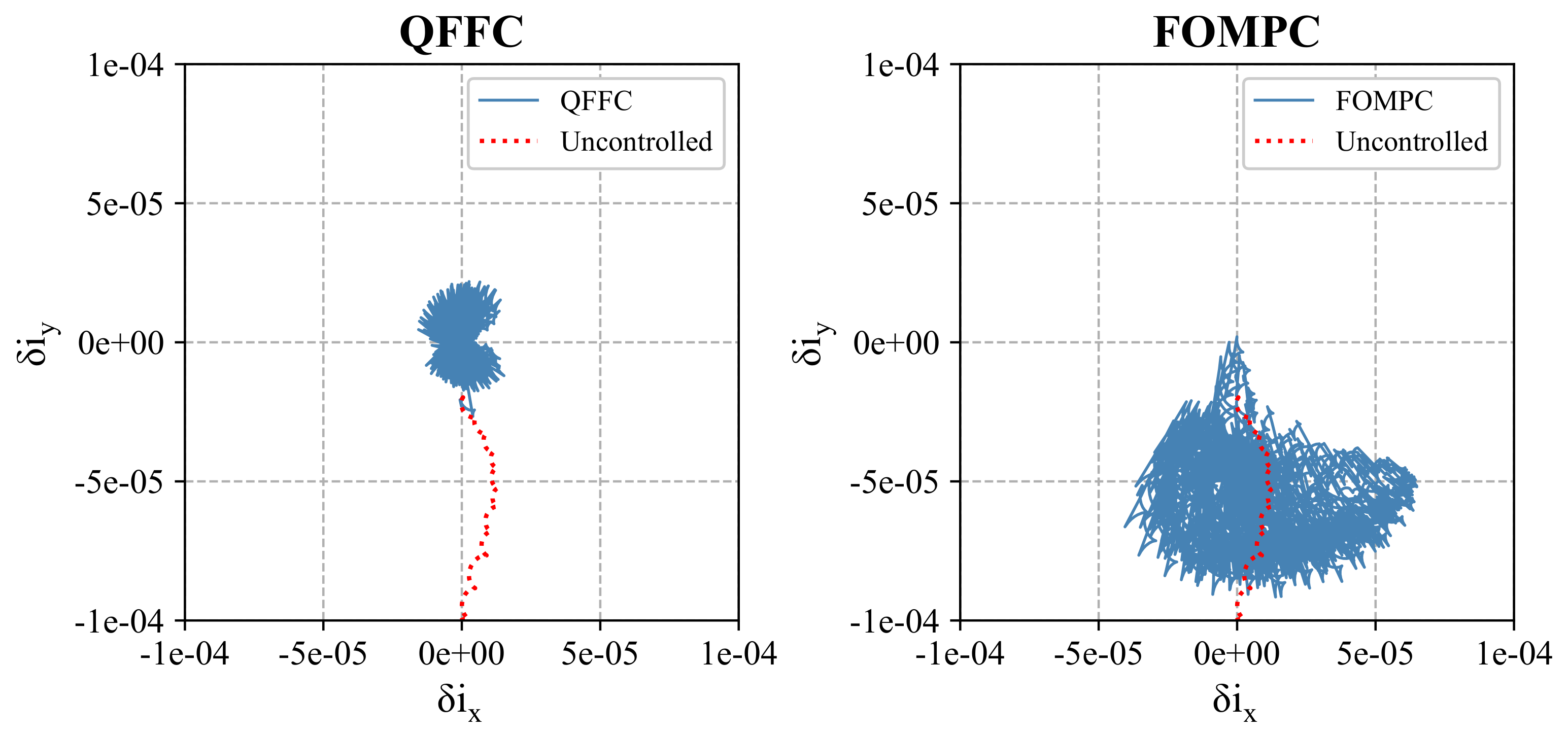
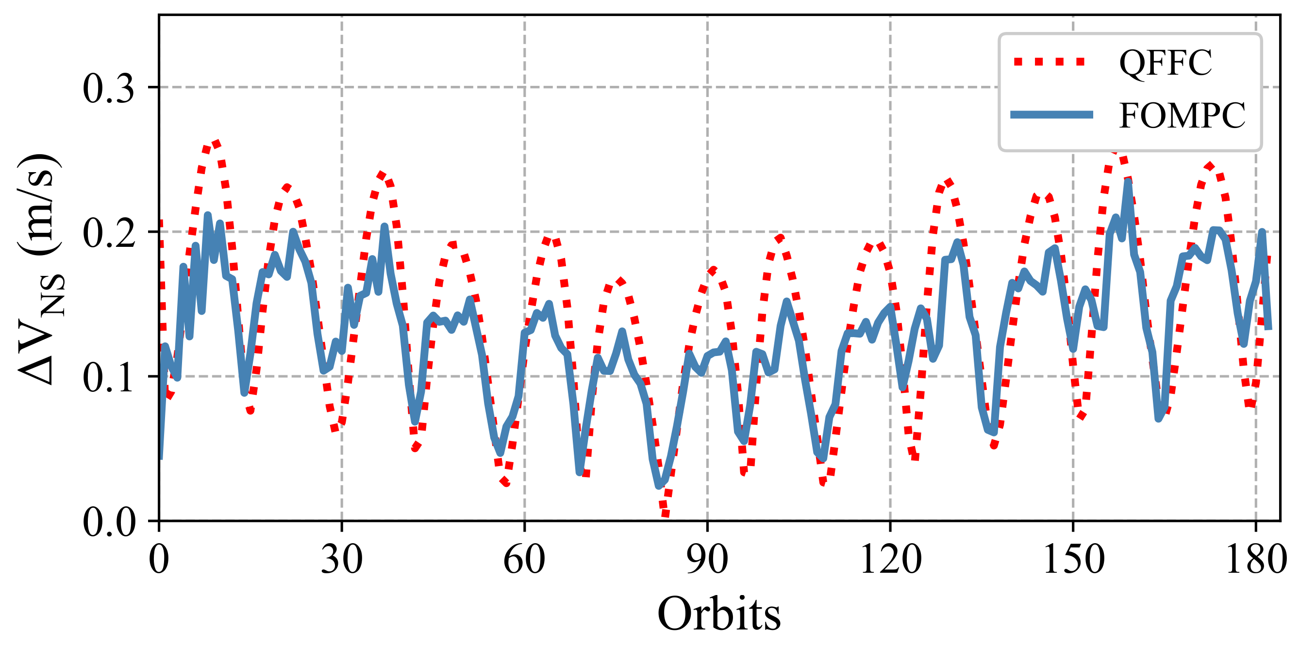
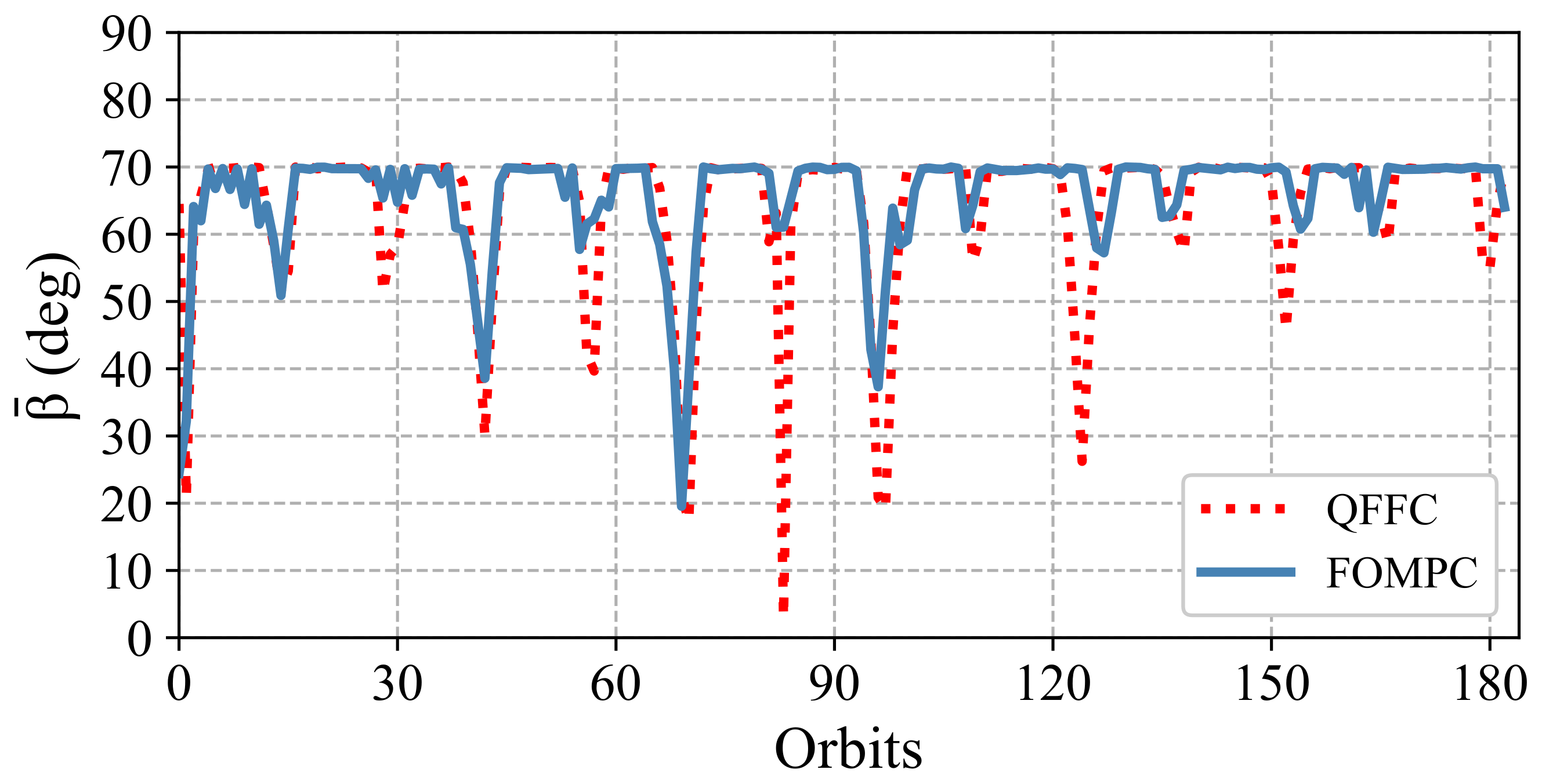
In this section, we present the results of several numerical simulations to test the QFFC and the FOMPC. Then, by setting different constraints and introducing the attitude and determination errors, we assess the robustness of the two controllers. To carry out simulations, we assume a testing environment with a GEO satellite of initial mass $m_0=5000\mathrm{kg}$. The satellite is equipped with two identical thrusters, which could generate the constant thrust of $F_{\mathrm{T}}=500\mathrm{mN}$ and have the specific impulse of $I_{\mathrm{sp}}=2250\mathrm{s}$. We will analyze the influence of different constraints and parameters in some simulations, while in other simulations, they are set to their nominal values, which are ${\beta }_{max}={70}^{\circ }$, ${\beta }_{min}=0^{\circ }$, ${\alpha }_{max}={60}^{\circ }$, ${\alpha }_{min}={30}^{\circ }$, $\Delta i_{max}=8\times {10}^{-5}$, and $N=6$. The dynamics and perturbations are stated in Section 2.2. Let the coefficients of the solar radiation pressure in Equation (4) be ${\rho }_{\mathrm{sun}}=4.5605\times {10}^{-6}\mathrm{N}/{\mathrm{m}}^2$, $\eta =0.6$, and $S=200{\mathrm{m}}^2$. The controllers are based on the mean elements, whereas the simulations are conducted by the high-precision orbit propagator with the osculating modified equinoctial elements. The start time of the mission is set to 12:00 on 1 January 2020, and the initial osculating elements of the GEO satellite are

$$\left\{p,f,g,h,k,L\right\}=\left\{42167,0,1\times {10}^{-4},0,5\times {10}^{-5},0.289893\right\}.$$

(43)

The objective elements are given by

$$\left\{{\lambda }_{\mathrm{T}},e_{x,\mathrm{T}},e_{y,\mathrm{T}},i_{x,\mathrm{T}},i_{y,\mathrm{T}}\right\}=\left\{{96}^{\circ },0,1\times {10}^{-4},0,3\times {10}^{-5}\right\}.$$

(44)

The algorithms are programmed in Fortran 90, and the testing platform is Intel^® Core™ i7-9700K 3.6 GHz. To be consistent with the previous studies, we measure the fuel consumption of station-keeping with the annual velocity increment ${\overline{V}}_{\mathrm{AN}}$.

5.1. Results

First, we carry out the one-year simulation for the two controllers. Figure 2 and Figure 3 present the time history of the osculating elements in the two simulations. Figure 4, Figure 5 and Figure 6 compare the trajectories in the $(\delta \lambda ,\delta \varphi )$, $(\delta e_x,\delta e_y)$, and $(\delta i_x,\delta i_y)$ plane, in which the red dashed line represents the trajectory in the uncontrolled situation. It’s obvious that without station-keeping, the satellite will quickly drift away from the objective. The results of the two simulations show that both the QFFC and the FOMPC could achieve long-term stable station-keeping with the ${\overline{V}}_{\mathrm{AN}}$ of $60.2\mathrm{m}/\mathrm{s}/\mathrm{year}$ and $54.2\mathrm{m}/\mathrm{s}/\mathrm{year}$, respectively. The number of maneuvers during 365 orbits of the QFFC and the FOMPC are 728 and 721, suggesting that each thruster performs approximately one maneuver per orbit. The QFFC and the FOMPC have almost the same performance in controlling the longitude and the eccentricity vector. According to Figure 4 and Figure 5, the control accuracy for the longitude and the eccentricity vector is about $\pm 0.013{}^{\circ }$ and $1.1\times {10}^{-4}$, respectively. The main difference between the two simulations is that the QFFC shows higher accuracy for controlling the inclination vector. That is because the QFFC requires the inclination vector to be fully adjusted to the objective at the end of each control cycle, while the FOMPC allows a certain deviation. Besides, Figure 3 shows that the inclination vector presents a more apparent periodic variation under the control of the FOMPC. To figure out the reason, we give Figure 7, which shows the half-year time history of the north–south velocity increment $\Delta V_{\mathrm{NS}}$ and Figure 8, which shows that of the average pitch angle $\overline{\beta }$. $\Delta V_{\mathrm{NS}}$ and $\overline{\beta }$ are given by

$$\Delta V_{\mathrm{NS}}=\left|V_{1}sin{\beta }_1\right|+\left|V_{2}sin{\beta }_2\right|$$

(45)

$$\overline{\beta }=arcsin\left(\frac{\Delta V_{\mathrm{NS}}}{V_1+V_2}\right).$$

(46)

Compared with the blue curve representing the FOMPC in Figure 7, the red one representing the QFFC shows a larger variation, reflecting the impact of the solar and lunar gravitational attraction. Meanwhile, according to Figure 8, $\overline{\beta }$ reaches its ceiling of ${70}^{\circ }$ most of the time in both simulations, indicating that the east–west velocity increment is usually forced to increase to adapt to the north–south velocity increment due to the constraint of the pitch angle. Therefore, by reducing the variation of $\Delta V_{\mathrm{NS}}$, the above situation may be avoided, thereby improving the efficiency of station-keeping, explaining how the FOMPC manages to save fuel consumption. However, this will allow the inclination vector to vary with the solar and lunar gravitational attraction, reducing the control accuracy of the inclination vector, as shown in Figure 6. The average CPU times per orbit of the QFFC and the FOMPC are 0.09 s and 57.4 s, respectively. Although the FOMPC has higher computational requirements, considering further code optimization and the upgrade of the computing system on the satellite, the on-board application of the FOMPC is possible.

Next, we conduct the following simulations concerning the impact of different parameters and constraints. Due to the characteristic of the optimization algorithm, the results of each simulation will be slightly different, even if the parameters are the same. Thus, we apply the Monte Carlo simulation method [43], in which we repeat the same simulation 20 times and take the average annual velocity increment as the ${\overline{V}}_{\mathrm{AN}}$. Figure 9, Figure 10, Figure 11 and Figure 12 present the simulations for the constraints of the yaw angle $\alpha$ and the pitch angle $\beta$. When we change one of these parameters, the others are assumed to be ${\beta }_{max}={90}^{\circ }$, ${\beta }_{min}=0^{\circ }$, ${\alpha }_{max}={90}^{\circ }$, ${\alpha }_{min}={90}^{\circ }$. The results show that the effects of ${\beta }_{max}$, ${\beta }_{min}$, ${\alpha }_{max}$, ${\alpha }_{min}$ on the QFFC and the FOMPC are almost the same. ${\beta }_{max}$ has the largest impact on the efficiency of station-keeping. As ${\beta }_{max}$ increases from ${45}^{\circ }$ to ${90}^{\circ }$, the ${\overline{V}}_{\mathrm{AN}}$ drops from $78.2\mathrm{m}/\mathrm{s}/\mathrm{year}$ to $57.5\mathrm{m}/\mathrm{s}/\mathrm{year}$ for the QFFC and $73.7\mathrm{m}/\mathrm{s}/\mathrm{year}$ to $51.4\mathrm{m}/\mathrm{s}/\mathrm{year}$ for the FOMPC. The drop is more apparent when ${\beta }_{max}$ is less than ${80}^{\circ }$, indicating that ${\beta }_{max}$ will remain a major limitation on the station-keeping efficiency until it reaches ${80}^{\circ }$. On the contrary, according to Figure 10, ${\beta }_{min}$ has almost no influence on the ${\overline{V}}_{\mathrm{AN}}$ until it reaches ${40}^{\circ }$. According to Figure 11 and Figure 12, ${\alpha }_{max}$ and ${\alpha }_{min}$ have the similar impact due to the symmetry. The restricted areas in the two figures represent the values of ${\alpha }_{max}$ and ${\alpha }_{min}$ with which the controllers could not operate stably. Outside the areas, the influences of ${\alpha }_{max}$ and ${\alpha }_{min}$ declines fast and becomes negligible after ${\alpha }_{max}$ and ${\alpha }_{min}$ reach ${45}^{\circ }$.

For the parameters N and $\Delta i_{\max }$ in the FOMPC, Figure 13 proves the existence of the optimal value of N, which are 3, 6, and 7 under weak, normal, and strong constraints. The detailed information of these three levels can be found in

Table 1. The values of ${\beta }_{max}$, ${\beta }_{min}$, ${\alpha }_{max}$, ${\alpha }_{min}$ in different levels of constraints.

Level	${\mathit{\beta }}_{max}$	${\mathit{\beta }}_{min}$	${\mathit{\alpha }}_{max}$	${\mathit{\alpha }}_{min}$
Weak	${90}^{\circ }$	$0^{\circ }$	${90}^{\circ }$	${90}^{\circ }$
Normal	${70}^{\circ }$	$0^{\circ }$	${60}^{\circ }$	${30}^{\circ }$
Strong	${60}^{\circ }$	$0^{\circ }$	${45}^{\circ }$	${25}^{\circ }$

. It is obvious that the optimal value of N goes up as the constraints get stronger, for the reason that strong constraints make the optimization more necessary. Figure 14 indicates that $\Delta i_{\max }$ significantly impacts the ${\overline{V}}_{\mathrm{AN}}$ because it determines the degree of optimization.

Finally we demonstrate the robustness of the two controllers by taking the attitude and determination errors into account. We assume that these disturbances follow the Gaussian distribution as

$$\chi \sim N\left({\chi }_{\mathrm{true}},{\sigma }_{\chi }^2\right)$$

(47)

where $\chi$ donates the yaw angle $\alpha$, the pitch angle $\beta$, the position vector $\mathbf{r}$, and the velocity vector $\mathbf{v}$, respectively, ${\chi }_{\mathrm{real}}$ is the true value, and ${\sigma }_{\chi }$ determines the error distribution range (EDR). We assume the nominal error distribution range (NEDR) of the attitude and determination as

$$\begin{array}{cc}\hfill 3{\sigma }_{\alpha ,\beta }& =0.{05}^{\circ }\hfill \\ \hfill 3{\sigma }_{\mathbf{r}}& =0.3\mathrm{m},\hfill \\ \hfill 3{\sigma }_{\mathbf{v}}& =5\times {10}^{-5}\mathrm{m}/\mathrm{s},\hfill \end{array}$$

(48)

which represents a high-accuracy level considering the present technology. Magnifying NEDR by $H_{\chi }$ times and applying them in the algorithm, we perform similar Monte Carlo simulations to investigate the influence of the errors of different types and different magnitudes. As shown in Figure 15, the attitude error has almost no effect on the two controllers. However, Figure 16 suggests that raising the EDR of the determination results in a significant increase of the ${\overline{V}}_{\mathrm{AN}}$. This is because the determination error directly affects the accuracy of the predictive model. For both the QFFC and the FOMPC, the station-keeping becomes unstable after $H_{\mathbf{r},\mathbf{v}}$ exceeds 800, indicating that the maximum EDR of the determination is $3{\sigma }_{\mathbf{r}}=240\mathrm{m},3{\sigma }_{\mathbf{v}}=0.04\mathrm{m}/\mathrm{s}$, which is closed to the accuracy of the on-board real-time GNSS determination [44]. In Figure 17, we also present the trajectories in the $(\delta \lambda ,\delta \varphi )$ plane with the maximum EDR of the determination. Compared with Figure 4, the control accuracy of the longitude has risen to $\pm 0.025{}^{\circ }$ for the QFFC and $\pm 0.030{}^{\circ }$ for the FOMPC. However, that of the latitude hardly changes, indicating that the stability of station-keeping for both the QFFC and the FOMPC is guaranteed under the condition of low determination accuracy.

5.2. Discussion

In the last part of this paper, we evaluate the performance of the QFFC and the FOMPC, considering the parameters and constraints of different values. Simulation results verify the validity of the QFFC and the FOMPC. Among all these parameters, ${\beta }_{max}$ has the most considerable influence on fuel consumption; ${\alpha }_{max}$, ${\alpha }_{min}$, and ${\beta }_{min}$ affect fuel consumption significantly only if the constraints are too strong. For the FOMPC, $\Delta i_{\max }$ determines the degree of optimization; the predictive horizon N has a certain impact, and the optimal value of N depends on how strong the constraints are. Robustness verification proves that both controllers could handle the attitude and determination errors of different magnitudes, while the rise of the determination error will cause extra fuel consumption. Here, we present

Table 2. The summary of our results and the comparison with those in the previous works.

	${\overline{\mathit{V}}}_{\mathbf{AN}}$$\left(\mathbf{m}/\mathbf{s}/\mathbf{year}\right)$	Controlling ${[{\mathit{e}}_{\mathit{x}},{\mathit{e}}_{\mathit{y}}]}^{\mathbf{T}}$ and ${[{\mathit{i}}_{\mathit{x}},{\mathit{i}}_{\mathit{y}}]}^{\mathbf{T}}$	Number of Thrusters	ON-OFF Thrusters	Number of Maneuvers Per Thruster Per Orbit
QFFC	60.2	Yes	2	Yes	0.997
FOMPC	54.2	Yes	2	Yes	0.988
[27]	78.6	No	4	Yes	-
[30]	59.4	No	6	No	-
[31]	66.8	No	4	Yes	2.98
[32]	72.3	Yes	-	Yes	-

, in which we summarize our results under normal constraints and compare them with those in the previous studies. The results prove that our approaches are effective.

6. Conclusions

Powered by advanced electric propulsion technology, the geostationary station-keeping problem using electric propulsion has attracted much attention. In this paper, we apply a novel thruster configuration involving two robotic arms. The QFFC and the FOMPC are proposed, and an NLMPC problem is solved. Both the QFFC and the FOMPC are proven to be effective in controlling multiple elements of the GEO satellite. The QFFC is capable of carrying out high-accuracy station-keeping with minor computational requirements, whereas the FOMPC could significantly reduce fuel consumption. Further investigations suggest that the parameters and constraints affect fuel consumption differently, among which the ceiling of the pitch angle of the thrust direction is the most influential parameter. The robustness assessments of the two controllers are also presented, considering the attitude and determination errors of different magnitudes. It proves that the two controllers are robust, but the rise of the determination error will cause extra fuel consumption.

Our study suggests that introducing robotic arms could benefit geostationary station-keeping significantly because it enables a wider range of the thrust direction, but its impact on the momentum management of the satellite is not involved in this paper. Next, the control problem that combines station-keeping and momentum management based on this thruster configuration will be our focus. Although the real application scenarios may be different from our assumptions, we expect our study to provide references for the control system design of GEO missions in the future.

References

1. Lemmens, M. Geo-Information: Technologies, Applications and the Environment; Springer Science & Business Media: Berlin/Heidelberg, Germany, 2011; Volume 5. [Google Scholar]
2. Finch, M.J. Limited space: Allocating the geostationary orbit. Nw. J. Int’l L. Bus. 1985, 7, 788. [Google Scholar]
3. Lee, B.S.; Lee, J.S.; Choi, K.H. Analysis of a station-keeping maneuver strategy for collocation of three geostationary satellites. Control Eng. Pract. 1999, 7, 1153–1161. [Google Scholar] [CrossRef]
4. Shrivastava, S.K. Orbital perturbations and stationkeeping of communication satellites. J. Spacecr. Rocket. 1978, 15, 67–78. [Google Scholar] [CrossRef]
5. Slavinskas, D.; Dabbaghi, H.; Benden, W.; Johnson, G. Efficient inclination control for geostationary satellites. J. Guid. Control Dyn. 1988, 11, 584–589. [Google Scholar] [CrossRef]
6. Jahn, R.G. Electric propulsion. Am. Sci. 1964, 52, 207–217. [Google Scholar]
7. Yang, G. Earth-moon trajectory optimization using solar electric propulsion. Chin. J. Aeronaut. 2007, 20, 452–463. [Google Scholar] [CrossRef] [Green Version]
8. Yang, D.; Xu, B.; Zhang, L. Optimal low-thrust spiral trajectories using Lyapunov-based guidance. Acta Astronaut. 2016, 126, 275–285. [Google Scholar] [CrossRef]
9. Takei, Y.; Saiki, T.; Yamamoto, Y.; Mimasu, Y.; Takeuchi, H.; Ikeda, H.; Ogawa, N.; Terui, F.; Ono, G.; Yoshikawa, K.; et al. Hayabusa2’s station-keeping operation in the proximity of the asteroid Ryugu. Astrodynamics 2020, 4, 349–375. [Google Scholar] [CrossRef]
10. Feuerborn, S.A.; Perkins, J.; Neary, D.A. Finding a way: Boeing’s all electric propulsion satellite. In Proceedings of the 49th AIAA/ASME/SAE/ASEE Joint Propulsion Conference, San Jose, CA, USA, 14–17 July 2013; p. 4126. [Google Scholar]
11. Jahn, R.G. Physics of Electric Propulsion; Courier Corporation: Honolulu, HI, USA, 2006. [Google Scholar]
12. Hofer, R. High-specific impulse operation of the BPT-4000 Hall thruster for NASA science missions. In Proceedings of the 46th AIAA/ASME/SAE/ASEE Joint Propulsion Conference & Exhibit, Nashville, TN, USA, 25–28 July 2010; p. 6623. [Google Scholar]
13. Sankovic, J.M.; Hamley, J.A.; Haag, T.W. Performance evaluation of the Russian SPT-100 thruster at NASA LeRC. In Proceedings of the IEPC Conference, Seattle, WA, USA, 13–14 September 1993. [Google Scholar]
14. Valentian, D.; Maslennikov, N. The PPS 1350 program. CP IEPC 1997, 97, 855–861. [Google Scholar]
15. Oleson, S.R.; Myers, R.M.; Kluever, C.A.; Riehl, J.P.; Curran, F.M. Advanced propulsion for geostationary orbit insertion and north-south station keeping. J. Spacecr. Rocket. 1997, 34, 22–28. [Google Scholar] [CrossRef] [Green Version]
16. Gomes, V.M.; Prado, A.F. Low-thrust out-of-plane orbital station-keeping maneuvers for satellites. Math. Probl. Eng. 2012, 2012, 532708. [Google Scholar] [CrossRef] [Green Version]
17. Gazzino, C.; Arzelier, D.; Losa, D.; Louembet, C.; Pittet, C.; Cerri, L. Optimal control for minimum-fuel geostationary station keeping of satellites equipped with electric propulsion. IFAC-PapersOnLine 2016, 49, 379–384. [Google Scholar] [CrossRef]
18. Gazzino, C.; Arzelier, D.; Cerri, L.; Losa, D.; Louembet, C.; Pittet, C. A three-step decomposition method for solving the minimum-fuel geostationary station keeping of satellites equipped with electric propulsion. Acta Astronaut. 2019, 158, 12–22. [Google Scholar] [CrossRef] [Green Version]
19. Gazzino, C.; Louembet, C.; Arzelier, D.; Jozefowiez, N.; Losa, D.; Pittet, C.; Cerri, L. Integer programming for optimal control of geostationary station keeping of low-thrust satellites. IFAC-PapersOnLine 2017, 50, 8169–8174. [Google Scholar] [CrossRef]
20. Gazzino, C.; Arzelier, D.; Louembet, C.; Cerri, L.; Pittet, C.; Losa, D. Long-term electric-propulsion geostationary station-keeping via integer programming. J. Guid. Control Dyn. 2019, 42, 976–991. [Google Scholar] [CrossRef]
21. De Bruijn, F.J.; Theil, S.; Choukroun, D.; Gill, E. Geostationary satellite station-keeping using convex optimization. J. Guid. Control Dyn. 2016, 39, 605–616. [Google Scholar] [CrossRef] [Green Version]
22. Min, W.; Qiang, L.; Xingang, L.; Ran, A. Electric Thrusters Configuration Strategy Study on Station-Keeping and Momentum Dumping of GEO Satellite. In Proceedings of the 2019 5th International Conference on Control Science and Systems Engineering (ICCSSE), Shanghai, China, 14–16 August 2019; pp. 115–121. [Google Scholar]
23. Guelman, M.M. Geostationary satellites autonomous closed loop station keeping. Acta Astronaut. 2014, 97, 9–15. [Google Scholar] [CrossRef]
24. Ruiz, J.L.; Frey, C.H. Geosynchronous satellite use of GPS. In Proceedings of the 18th International Technical Meeting of the Satellite Division of the Institute of Navigation (ION GNSS 2005), Long Beach, CA, USA, 13–16 September 2005; pp. 1227–1232. [Google Scholar]
25. Yang, W.; Li, S. A station-keeping control method for GEO spacecraft based on autonomous control architecture. Aerosp. Sci. Technol. 2015, 45, 462–475. [Google Scholar] [CrossRef]
26. Park, B.K.; Tahk, M.J.; Bang, H.C.; Park, C.S.; Jin, J.H. A new approach to on-board stationkeeping of geo-satellites. Aerosp. Sci. Technol. 2005, 9, 722–731. [Google Scholar] [CrossRef]
27. Garcia, C.E.; Prett, D.M.; Morari, M. Model predictive control: Theory and practice-A survey. Automatica 1989, 25, 335–348. [Google Scholar] [CrossRef]
28. Weiss, A.; Di Cairano, S. Opportunities and potential of model predictive control for low-thrust spacecraft station-keeping and momentum-management. In Proceedings of the 2015 European Control Conference (ECC), Linz, Austria, 15–17 July 2015; pp. 1370–1375. [Google Scholar]
29. Weiss, A.; Kalabić, U.; Di Cairano, S. Model predictive control for simultaneous station keeping and momentum management of low-thrust satellites. In Proceedings of the 2015 American Control Conference (ACC), Chicago, IL, USA, 1–3 July 2015; pp. 2305–2310. [Google Scholar]
30. Walsh, A.; Di Cairano, S.; Weiss, A. MPC for coupled station keeping, attitude control, and momentum management of low-thrust geostationary satellites. In Proceedings of the 2016 American Control Conference (ACC), Boston, MA, USA, 6–8 July 2016; pp. 7408–7413. [Google Scholar]
31. Weiss, A.; Kalabić, U.V.; Di Cairano, S. Station keeping and momentum management of low-thrust satellites using MPC. Aerosp. Sci. Technol. 2018, 76, 229–241. [Google Scholar] [CrossRef]
32. Caverly, R.J.; Di Cairano, S.; Weiss, A. Electric Satellite Station Keeping, Attitude Control, and Momentum Management by MPC. IEEE Trans. Control Syst. Technol. 2020, 29, 1475–1489. [Google Scholar] [CrossRef]
33. Zou, H.; Song, J.; Wang, J.; Zhang, L.; Huang, Y. Geostationary Station Keeping Using Relative Orbital Elements with Model Predictive Control. In Proceedings of the 2020 Chinese Control And Decision Conference (CCDC), Hefei, China, 22–24 August 2020; pp. 4437–4442. [Google Scholar]
34. Boniface, C.; Charbonnier, J.M.; Lefebvre, L.; Leroi, V.; Lienart, T. An overview of electric propulsion activities at CNES. In Proceedings of the 35th International Electric Propulsion Conference, Atlanta, GA, USA, 8–12 October 2017. [Google Scholar]
35. Sembély, X.; Wartelski, M.; Doubrère, P.; Deltour, B.; Cau, P.; Rochard, F. Design and Development of an Electric Propulsion Deployable Arm for Airbus Eurostar E3000 ComSat Platform. In Proceedings of the 35th International Electric Propulsion Conference, Atlanta, GA, USA, 8–12 October 2017. [Google Scholar]
36. Curtis, H. Orbital Mechanics for Engineering Students; Butterworth-Heinemann: Oxford, UK, 2013. [Google Scholar]
37. De Ruiter, A.H.; Damaren, C.; Forbes, J.R. Spacecraft Dynamics and Control: An Introduction; John Wiley & Sons: Hoboken, NJ, USA, 2012. [Google Scholar]
38. Walker, M.; Ireland, B.; Owens, J. A set modified equinoctial orbit elements. Celest. Mech. 1985, 36, 409–419. [Google Scholar] [CrossRef]
39. Li, L.; Zhang, J.; Zhao, S.; Qi, R.; Li, Y. Autonomous onboard estimation of mean orbital elements for geostationary electric-propulsion satellites. Aerosp. Sci. Technol. 2019, 94, 105369. [Google Scholar] [CrossRef]
40. Boyd, I.D. Numerical modeling of spacecraft electric propulsion thrusters. Prog. Aerosp. Sci. 2005, 41, 669–687. [Google Scholar] [CrossRef]
41. Bazaraa, M.S.; Sherali, H.D.; Shetty, C.M. Nonlinear Programming: Theory and Algorithms; John Wiley & Sons: Hoboken, NJ, USA, 2013. [Google Scholar]
42. Sahin, K.H.; Ciric, A.R. A dual temperature simulated annealing approach for solving bilevel programming problems. Comput. Chem. Eng. 1998, 23, 11–25. [Google Scholar] [CrossRef]
43. Mooney, C.Z. Monte Carlo Simulation; Sage: New York, NY, USA, 1997; Number 116. [Google Scholar]
44. Xiong, Z.; Qiao, L.; Liu, J.; Jiang, B. GEO satellite autonomous navigation using X-ray pulsar navigation and GNSS measurements. Int. J. Innov. Comp. Inform. Control 2012, 8, 2965–2977. [Google Scholar]
Figure 1. Model of a satellite in the RSW coordinate system applying the thruster configuration with robotic arms.
Aerospace 09 00182 g001
Figure 2. Time history of the osculating elements in the one-year simulation for the QFFC.
Aerospace 09 00182 g002
Figure 3. Time history of the osculating elements in the one-year simulation for the FOMPC.
Aerospace 09 00182 g003
Figure 4. The comparison of the trajectories in the ( δ λ , δ ϕ ) plane.
Aerospace 09 00182 g004
Figure 5. The comparison of the trajectories in the ( δ e x , δ e y ) plane.
Aerospace 09 00182 g005
Figure 6. The comparison of the trajectories in the ( δ i x , δ i y ) plane.
Aerospace 09 00182 g006
Figure 7. The half-year time histories of Δ V NS for the QFFC and the FOMPC.
Aerospace 09 00182 g007
Figure 8. The half-year time histories of β ¯ for the QFFC and the FOMPC.
Aerospace 09 00182 g008
Figure 9. The results of Monte Carlo simulations for β max .
Aerospace 09 00182 g009
Figure 10. The results of Monte Carlo simulations for β min .
Aerospace 09 00182 g010
Figure 11. The results of Monte Carlo simulations for α max .
Aerospace 09 00182 g011
Figure 12. The results of Monte Carlo simulations for α min .
Aerospace 09 00182 g012
Figure 13. The results of Monte Carlo simulations for the prediction horizon N under different levels of constraints.
Aerospace 09 00182 g013
Figure 14. The results of Monte Carlo simulations for Δ i max .
Aerospace 09 00182 g014
Figure 15. The results of Monte Carlo simulations for the attitude error of different magnitudes.
Aerospace 09 00182 g015
Figure 16. The results of Monte Carlo simulations for the determination error of different magnitudes.
Aerospace 09 00182 g016
Figure 17. The trajectories in the ( δ λ , δ ϕ ) plane considering the maximum EDR of the determination.
Aerospace 09 00182 g017