1. Introduction
The aviation industry estimated a steady growth across Europe over the years, mainly due to the increase in tourism and cargo demand. The base scenario forecast was 1.8 million Instrument Flight Rules (IFR) movements in Europe in 2021, 9.6% more than in 2018 [
1]. At the time of this writing, aviation exhibits an unprecedented decrease in traffic due to COVID-19. However, early recovery is expected [
2], and when the aviation industry returns to “normal” conditions, the airspace will most likely exhibit the same capacity deficit.
In the current European air transportation network, the airspace user (AU) enjoys high flexibility in the flight planning process. It is required to submit the final flight plans between 120 and 3 h before the flight, providing them the advisability to account for uncertain factors, such as aircraft availability or convective weather [
3]. Therefore, the accurate number of flights, at what time, and where, is known on the Day of Operation (D0). To ensure successful distribution of flights, Air Navigation Service Providers (ANSPs) start defining their capacities a year to six months prior to D0. Maximum capacity values are typically estimated based on historical traffic levels, geometrical characteristics of the airspace, Air Traffic Controller (ATCO) workload models, staff availability, or convective weather [
4].
This deviation between the expected number of flights (demand) and the forecasted capacity can result in demand–capacity imbalances, generating delays, flight-level constraints, or forcing re-routing. Earlier information sharing on flight intentions could help both AU and ANSPs obtain better Demand–Capacity Balancing (DCB). However, when those imbalances between demand and capacity cannot be resolved through airspace management or flow management solutions, the ANSPs, through the Flow Manager Position (FMP), and Network Manager (NM) operators, agree on Air Traffic Flow Management (ATFM) regulations [
5]. These regulations shall apply the required constraints to reduce the demand over the overloaded part of the network, ensuring the available airspace capacity meets the traffic demand, together with a safe and ordered flow of air traffic.
Most ATFM regulations are applied to specific Traffic Volumes (TVs), which can be informally defined as a portion of airspace. Formally, a TV is an environment data structure, associated to only one reference location based on geographical entities (e.g., sector, collapsed sectors, or airports), and they are used to compare the traffic load and the available capacity [
6].
Because the process of identifying possible demand–capacity imbalances and applying the required ATFM regulations is done along several months, the ATFM provision in the European Civil Aviation Conference (ECAC) region is carried out in four phases [
6]:
Strategic flow management takes place seven days or more prior to the D0. This phase focuses on continuous data collection with a review of measures directed towards the early identification of major DCBs. The output of this phase is the Network Operations Plan (NOP);
Pre-tactical flow management is applied during the six days prior to the D0. This phase studies the demand for the day of the operation, comparing it with the predicted available capacity, and makes any necessary adjustments to the NOP. The output is the ATFCM Daily Plan (ADP);
Tactical flow management takes place on the D0 and involves considering, in real-time, those events that affect the ADP and making the necessary modifications to it. This phase aims at ensuring that the measures taken during the previous ones are the minimum required;
Post operational analysis takes place following the tactical phase. During this phase, an analytical process is carried out that measures, investigates, and reports on operational processes relevant to ATFM measures. The final result of this phase is the development of best practices to improve operational processes and activities.
From the previous phases, it can be seen that the Dcb process has two steps: the
detection of demand–capacity imbalances and the
resolution of them. Examples of Atfm systems [
6] used throughout the previous phases include the Enhanced Tactical Flow Management System (ETFMS), which compares traffic demand, regulated demand, and load against capacity to assess possible imbalances in the airspace. The PREDICT system compares forecasted traffic and capacity to evaluate the load situation for the following days (up to 6 days in advance). Moreover, ATFM measures may be implemented in this system to assess their impact before being applied. Similarly, SIMulation and EXperiment (SIMEX), used in strategic, pre-tactical, and tactical phases, enables Network Operations staff to simulate ATFM measures or restrictions. The NOP portal and the Collaboration Human Machine Interface (CHMI) interface allow real-time data sharing and enable Collaborative Decision Making (CDM) between all partners. Finally, ATFM delays are imposed on flights that plan to use overloaded resources, considering a First Planned—First Served principle as defined by the Computer Assisted Slot Allocation (CASA) algorithm [
6].
Despite the huge variety of metrics, tools, and systems used during the different ATFM phases, in the past five years, en-route delay accounted for 50–60% of total ATFM delay [
2]. Furthermore, the methodology used nowadays is purely human and does not rely on automation. Decision-making on traffic surveillance, conflict detection, and conflict resolution are all processes done in the controller’s mind by building up a mental picture of the flights’ intent [
7]. Moreover, the FMPs have to consider that, in realistic operations, a certain amount of capacity overloads are usually allowed [
8]. Several reasons could explain this phenomenon: the lack of initial schedules for non-planed flights, the use of entry rate for assessing the demand without considering the occupancy, or a conservative approach for estimating the capacity and the complexity.
In this context, the introduction of new controller support tools for the
detection phase of the DCB process could reduce the amount of work, or at least the difficulty, of the FMPs tasks, and it could even result in a capacity increment. In a previous work [
9], we dealt with the development of a Recurrent Neural Network (RNN) and and a Convolutional Neural Network (CNN) capable to replicate the human decisions made to detect C-ATC Capacity ATFM regulations, for en-route traffic, at the TV level, and over the MUAC region (Maastricht Upper Area Control Centre). In this previous work, we showed how ML models can learn from past scenarios when the demand was allowed above/under the capacity and use the knowledge in future predictions.
Although the
RNN-based model achieved the maximum recall, the
CNN-based model outperformed it in terms of precision. Due to the excellent performance of both models independently, in this article we will study whether there is a hybrid model that can take advantage of the best of each individual model and increase precision while maintaining high recall. Three different hybrid architectures are studied, the
RNN-CNN cascade model (see
Figure 1) becoming the best option. This novel framework is evaluated over the MUAC and the REIMS regions. Moreover, a deep analysis of its behavior is performed to understand the reasons behind the predictions, crucial to ensure compliance with company policies, industry standards, and government regulations.
Therefore, this article address (i) the utilization of Deep Learning (DL) models to replicate the process done by the FMPs to detect demand–capacity imbalances, (ii) explores three different hybrid models for pre-tactical phase, (iii) focuses on two of the most regulated European regions, (iv) presents the obtained results, and (v) studies the utilization of Explainable Artificial Intelligence (XAI) tools to allow humans understand the predictions done by the models.
2. State of the Art
Following pioneer work done by [
10] to improve ATFM performance, previous research has focused on identifying regions with demand–capacity imbalances and required operational constrains. The literature shows three main trends: proposals without any Artificial Intelligence (AI), approaches using supervised Machine Learning (ML), or works exploring Reinforcement Learning (RL) techniques.
All three families are present in the SESAR 2020 Exploratory Research program, which is leading the investigation into the future of ATFM in Europe. For instance, the COTTON (Capacity Optimisation in TrajecTory-based OperatioNs) project [
11] focus on the DCB processes regarding airspace management without using AI. On the other hand, using (AI), the ISOBAR (Artificial Intelligence Solutions to Meteo-Based DCB Imbalances for Network Operations Planning) project [
12] aims at the integrating enhanced convective weather forecasts for predicting imbalances between capacity and demand. Additionally, the DART (Data-driven aircraft trajectory prediction research) project [
13] exploits RL techniques to solve possible demand–capacity imbalances.
In Air Traffic Management (ATM), many other approaches have been studied for the DCB problem without using AI. For instance, ref. [
14] presents a spatio-temporal model, driven by discrete events, to simulate and validate the departure-time-bounded adjustment process that preserves the scheduled slots, to reduce, or solve, demand–capacity imbalances. Ref. [
15] presents a dynamic sectorization to adjust capacity to demand. Ref. [
16] proposes both modifications of trajectories to adjust demand and opening schemes to adjust sectorizations to demand.
Similarly, several papers address mathematical models for an anticipatory, time-dependent modulation of Air Navigation Services (ANSs) charges, aiming to alleviate the demand-capacity imbalance on an airspace network at minimal cost [
17], planning to redistribute the traffic across the network so as to respect nominal airspace and airport capacities [
18], or to achieve redistribution of peak-load traffic [
19].
Related to the DCB problem, research has been undertaken on traffic complexity metrics with the aim of capturing the main features explaining the air traffic controller workload. Ref. [
20] is a recent summary of the most studied complexity indicators as a contributory factor in charge of controllers’ workload. In [
21,
22], the authors demonstrated that fairly basic metrics (such as occupancy count, entry count, vertical speed, or speed-vector interactions) have a high correlation to the sector status when having a macroscopic observation of the workload. Moreover, many of the more complex metrics turned out to be redundant with respect to the basic ones. In [
23], a dynamic approach to capture complexity was presented using time windows, rather than using a single score. Despite the four complexity indicators described that combine spatiotemporal topological information with the severity of the interdependencies, the authors manifest the need of mapping between the indicators and controller workload. They also highlight the importance of how this information is presented to the controllers.
On the other hand, little research has been conducted to improve the current DCB process using supervised ML models. In [
22], the author presents a supervised neural network that takes relevant air traffic complexity metrics as input and provides a workload indication (high, normal, or low) for any given Air Navigation Services (ANSs) sector. Then, tree search methods are used to explore all possible combinations of elementary airspace modules in order to build an optimal airspace partition where the workload is balanced as well as possible across the ATC sectors. The INTUIT project is related to ATFM regulations using ML and visual analytics. In [
24], the authors focus on analyzing the spatio-temporal patterns of ATFM delays in the European network. Also related to predicting delays, ref. [
25] face the challenge of predicting the total network delay using analytical methods, optimization approaches, and a Deep Convolutional Neural Network (DCNN).
Notice that the previous works are related to the DCB problems or ATFM regulations, but none of them focus explicitly, or exclusively, on their detection. To close this gap, in [
9], we demonstrated the potential to detect the need of ATFM regulations under the current ATM environment. We have shown that both a CNN and a RNN can be used to predict C-ATC Capacity ATFM regulations with 90% accuracy.
Last but not least, regarding the CDM process to identify and solve demand–capacity imbalances using RL, researchers have explored different approaches to incorporate mechanisms to further improving ATFM performance. Ref. [
26] presents a fairness metric to measure deviation from first-scheduled, first-served in the presence of conflicts. Similarly, ref. [
27] propose a discrete optimization model that attempts to incorporate an equitable distribution of delays among airlines by introducing a notion of fairness. Ref. [
28] simulated the involvement of ATM stakeholders in the CDM process using agent-based models.
Related to agent-based models to specifically improve ATFM, ref. [
29] developed a multi-agent system in a grid computing environment to deal with the problem of ATFM synchronization, focusing on congestion identification, conflicts resolution and agreements negotiation. Additionally, ref. [
30] formalizes the problem as a multi-agent Markov Decision Process (MDP) towards deciding flight ground delays to resolve imbalances, during the pre-tactical phase. The DART project, mentioned above, is composed of a data-driven trajectory prediction and agent-based collaborative learning [
31].
Three relevant aspects of these RL approaches are that (a) the approach used to detect the demand–capacity imbalances is very poor and unrealistic due to it is not the main goal, (b) they focus on the resolution of demand–capacity imbalances, and (c) they are introducing a new paradigm of behavior.
To work around the limitations identified in the literature, we propose to explicitly focus on the detection of ATFM regulations, trying to replicate the decisions made by the FMPs. This approach aims to create a support tool to help detect more efficiently and faster possible ATFM regulations due to demand–capacity imbalances. To do it, we propose to study different hybrid ml models, which has proved excellent performance in other fields. In [
32], a hybrid network model based on CNN and Long-Short Term Memory (LSTM), is used to forecast power demand. In [
33], a hybrid classification model, also based on CNN and LSTM, reported an accuracy of 98.37% detecting spam messages.
3. Methodology
This section aims to describe the different Neural Network (NN) architectures proposed in this work. First, we formalize the research questions we want to answer and its assumptions. Second, we describe the characteristics of the input samples and the two levels of granularity that the output of the models can offer. Third, we describe the RNN-based model, which uses scalar variables as input, and the CNN-based model, that uses artificial images. Finally, we present the architecture of three different hybrid models that result from combining the previous ones.
3.1. Research Questions and Assumptions
The main goal of this research is to provide a support tool based on DL techniques to help the operator decide if a regulation is needed on a particular TV at a given time. Based on previous results [
9], this work aims to answer several research questions. First, we want to investigate if a combination of RNN and CNN can be used to improve performance. To do this, we will evaluate three different hybrid architectures. Second, we question whether it is necessary to train a specialized model for each TV or a general model can be used for all of them. Third, we want to validate that the proposed architecture works for different regions. To this end, we have extended the study to the REIMS region, one of the most regulated areas. Finally, we want to study which input variables are the most relevant for the models and analyze the behavior of those models. For this purpose, we will use XAI tools.
An inherent assumption in supervised learning is that noise in input features and labels is low. In our case, it is assumed that the data in the AIRACs is accurate and that the decision to apply or not apply a regulation was correct. Supervised models learn patterns from historical data and use them in future predictions. In that sense, our models will not improve the decisions made in the past. However, DL models also have the ability to improve learning as the quantity and quality of data increases, and thus will benefit as better quality data become available or improved ATFCM algorithms emerge. Another usual assumption in ML is that non-modeled features have negligible effects. Our data contains features that are primarily correlated with regulations according to previous publications [
22], even though not all possible complexity indicators related to ATFM regulations are used (e.g., number of available controllers). Additional information related to the air traffic complexity is also inherent in the images data.
3.2. Inputs and Outputs of the Models
The developed frameworks use two types of input samples.
Scalar variables for the time-distributed RNN, and
artificial images for the time-distributed CNN. In both cases, we extract the information/data from the AIRACs (detailed description of the airspace configuration for a specific period) used in the R-NEST (model-based simulation tool), and generate samples of 30-min intervals sliced into one-minute time-steps (see
Figure 2 as a visual reference).
There are three main reasons behind using 30-min intervals. First, to our best knowledge, ATCOs look look at a minimum interval, between fifteen and thirty min, when considering the implementation of ATFM regulations. Second, we want to predict possible ATFM regulations for specific intervals of time (e.g., “Is needed a regulation from 7 a.m. to 10:30 a.m. on 12 September?”), and also for a given entire day (e.g., “What are the regulations required for 12 September?”). Third, we want to identify, as precisely as possible, the moment a regulation shall start and end. Moreover, as we will see in
Section 4.1, the average duration of regulation is 110 min. Therefore, we must select an appropriate interval length to have samples showing the transition between no-regulated and regulates intervals (and vise versa), purely no-regulated intervals, and completely regulated.
The generation of each interval starts at a random timestamp to avoid any possible bias. And to label each of the time-steps, we used the C-ATC Capacity ATFM regulations for en-route traffic provided by EUROCONTROL.
On the other hand, the outputs of the models can have two levels of granularity, depending on whether the predictions are made at the time-step level or at the interval level. At the time-step level, each input time-step is classified as positive (regulation needed) or negative (no regulation needed). However, knowing exactly the time steps to regulate may be a too-fine granularity for the current CDM process. Furthermore, predicting the exact time when a regulation will start and end is a challenging task. To this end, the models’ output can be evaluated at the interval level, where an input sequence of consecutive time-steps is classified as positive or negative.
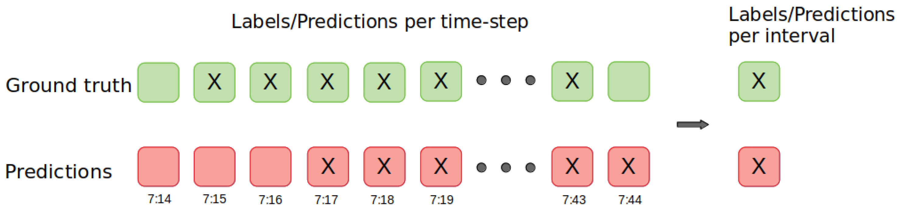
Specifically, the
interval classification is based on grouping the ground truth and the predictions to determine whether the 30 min interval contains a regulation or not (see
Figure 3). An interval is considered to have a regulation if the number of positive time-steps in the interval is above a given threshold. In this evaluation, the threshold is set to five time-steps for two reasons. First, by the nature of the application, we consider false-negatives (no detecting a needed regulation) to be more critical than false-positives (predict a regulation that is not needed), that can be filtered later by the operator. Second, we want to avoid isolated positive time-steps (misunderstandings of the model).
3.3. RNN-Based Model
The main characteristic of plRNN is the fact they are able to exhibit temporal dynamics because information travels in loops from layer to layer. So, the state of the model is influenced by its previous states. We tested different RNN architectures, such as Gated Recurrent Units (GRU) and and purely RNN’s cells, however, the best results were obtained using LSTM cells (the reader may refer to [
34] for a more thorough view of LSTM).
The input
scalar variables used for the
RNN-based model can be directly exported from R-NEST. We decided to use a combination of the most basic scalar variables and those presented in [
22] as the most representative to exhibit the traffic’s complexity:
“Timestamp” (associated 30 min interval of the studied day—from 0 to 48);
Capacity;
Occupancy count;
Entry count for the next 20 and 60 min;
Expected workload;
Number of conflicts;
Number of flights at the different phases (climbing, cruising and descending).
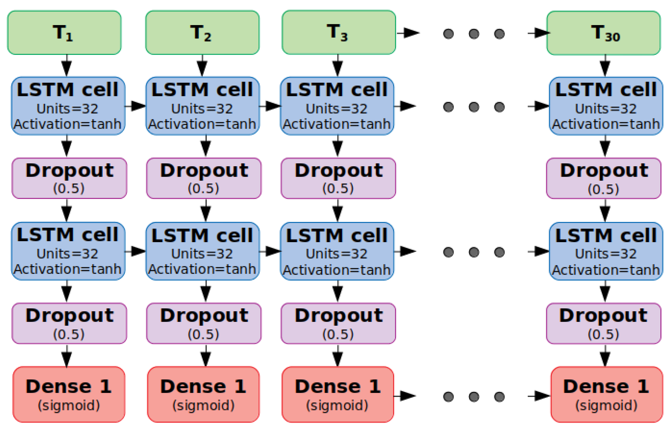
Common LSTM are designed to provide a single prediction for the input sequence. However, we want to obtain a prediction for each of the input time-steps. For this reason, each LSTM cell returns the entire sequence, and the output layer is composed of a dense layer with a time-distributed wrapper. The time-distributed wrapper allows us to process the extracted features per time-step with the same set of weights and obtain a binary prediction for each of them.
As we want a RNN able to make a prediction for each of the input time-steps, the model could be prone to overfitting. This commonly happens when a model has more parameters than necessary to express the patterns inside the input data. One method to reduce overfitting is dropout. At each training stage, individual nodes are kept with probability p or “dropped out” of the network (ignored) with probability 1 − p. Only the reduced network is trained on the data in that stage, and therefore, it is less likely to exhibit overfitting. It increases the model’s ability to generalize.
Figure 4 is a graphical representation of the architecture used.
3.4. CNN-Based Model
Every TV has different characteristics not only in terms of the features used for the RNN-based model, but also critical points, standard arrival and departure flows, aircraft groupings, etc. This information is not in the source of information used (AIRACs). However, they could be figured out by the models from input images representing the exact configuration of each TV and how the flights are distributed. In a way, these artificial images are intended to provide additional information related to the complexity of the particular situation.
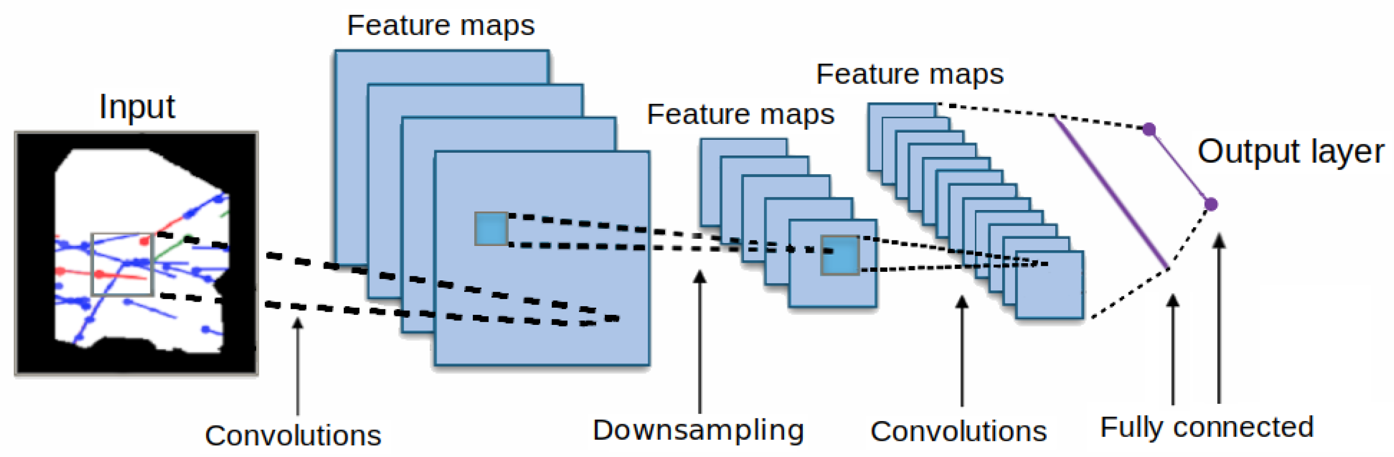
CNNs are the most popular and widely used technique to analyze static visual imagery. The convolutional layer is the core block of a CNN. This layer uses a set of filters (or kernels), which are convolved across the entire width and height of the volume, to create a 2-dimensional activation map. The final output volume of a CNN layer consists of stacking the activation maps, for all the filters, along the depth dimension to form the output volume. As a result, the CNN network learns filters that activate when it detects some specific type of feature at some spatial position in the input (see
Figure 5 as an example).
After the convolutional layer, most conventional CNNs include local and/or global pooling layer. They are used to reduce the dimensionality of data, and hence to also control overfitting (“memorization”), by combining the output from multiple neurons into a single neuron into the next layer. There are two common types of pooling layers: max pooling and average. Max pooling uses the maximum value of each local cluster of neurons in the feature map, while average pooling takes the average value. Finally, after some convolutional and pooling layers, the final classification is done via a fully connected layer, where neurons from previous layers have connections to all neurons in the next layer.
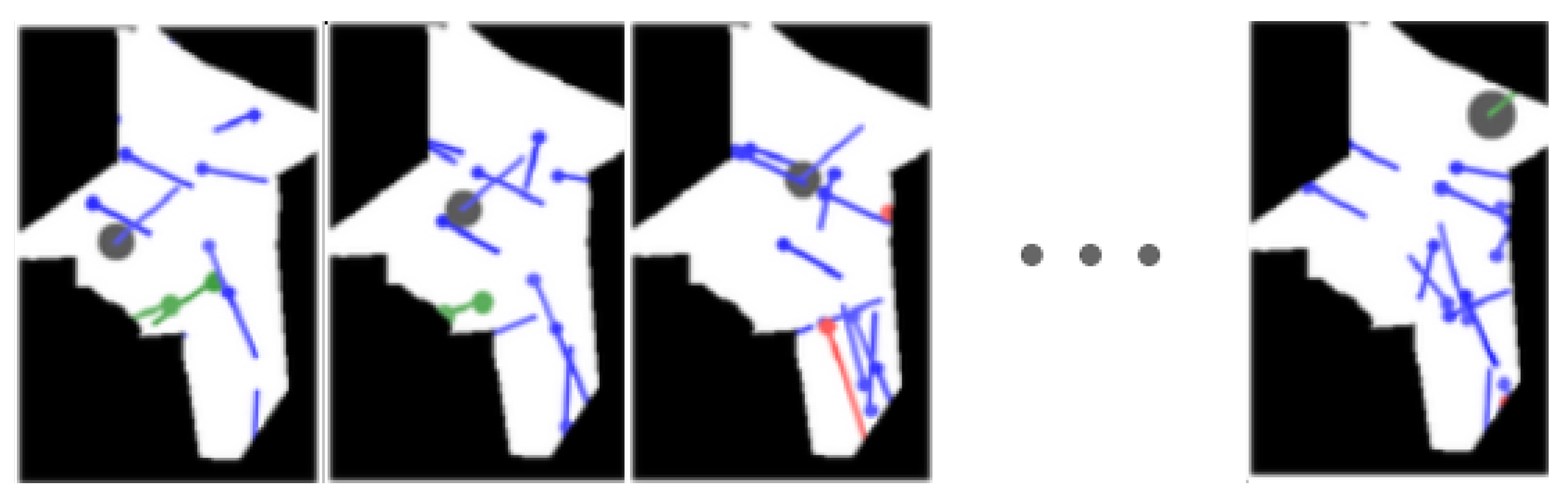
In our case, we want a
CNN-based model able to process images that evolve on time. Therefore, our input samples are sequences of images showing the airspace configuration at consecutive time-steps (see
Figure 6).
The sequences of images are artificially generated using the trajectory file available in the AIRAC. The sampling rate of these trajectories is not constant, often providing more data points (aircraft ID, date/time, latitude, longitude, Flight Level-FL) during the departure and arrival phases of a flight than at the cruising phase. By making the assumption of constant speed between data point, we can interpolate the trajectories (see [
35] as another example of interpolation), and obtain both the location (latitude, longitude, FL) and heading of each aircraft inside a TV in a particular time-step. Finally, to represent the shape of the TV, from the file
Newmaxo ASCII Region file, we extracted the set of pairs (latitude, longitude) that define the perimeter of a TV.
Furthermore, to increase the number of samples, and also reduce possible overfitting, we used data augmentation (see [
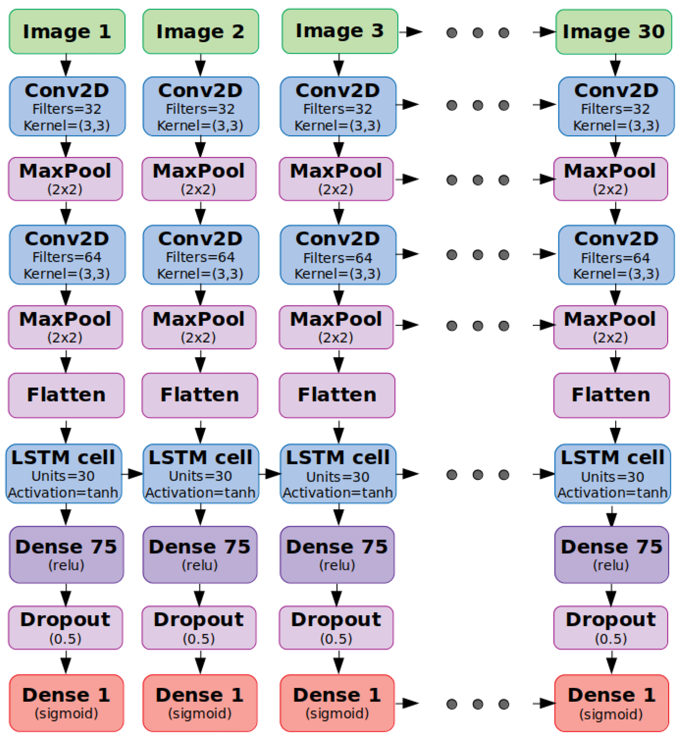
36] for further details). Concretely, we apply transformations such as random horizontal and vertical flip, clipped zoom, and rotations. Taking into account all the previous information, we developed an architecture equivalent to
Figure 7, which can capture the temporal evolution of the airspace since the images per set are processed in parallel using the time-distributed wrapper.
3.5. RNN-CNN Hybrid Model
The final framework proposed to detect C-ATC Capacity ATFM regulations is a hybrid model, which combines the two previous ones and takes advantage from both the RNN-based model, which processes more general metrics, and the CNN-based model, able to process the specific airspace configuration.
The main reason for using this framework is the fact that individual models exhibit low precision compared to the reported high accuracy and recall (see
Section 4.3 and
Section 4.4). The precision refers to the proportion of correctly identified regulations; therefore, we want to reduce the false-positive predicted time-steps. Moreover, these architectures increases the overall performance concerning the individual ones.
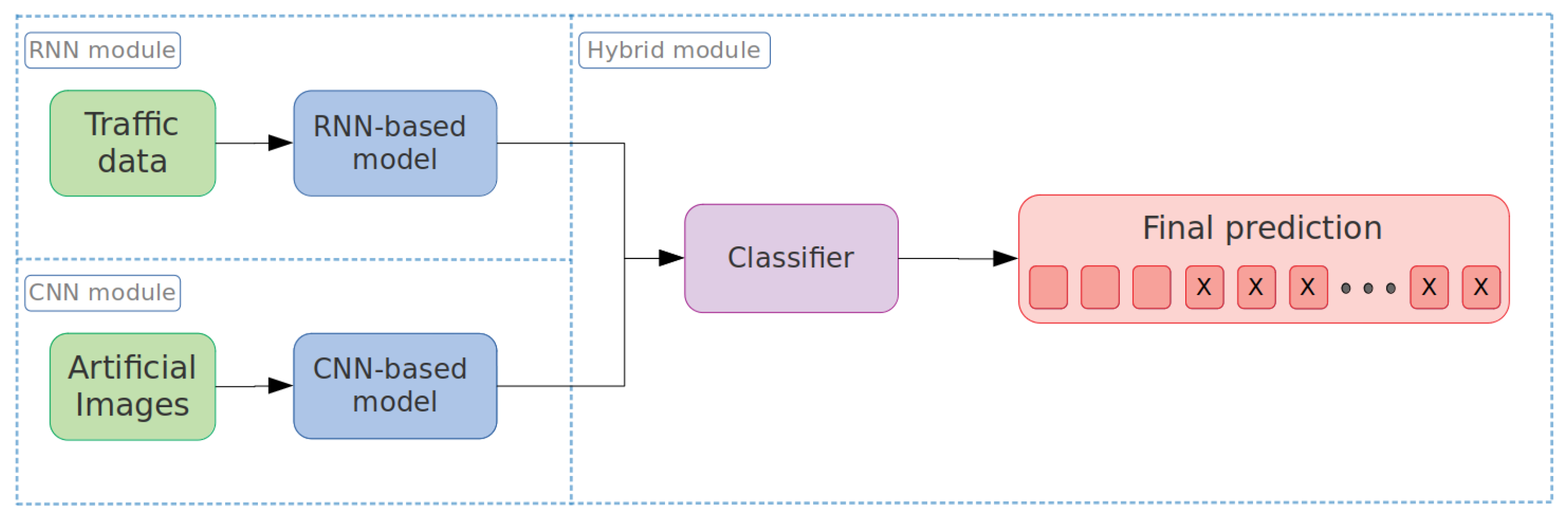
To refine the positive predictions and reduce the false-positives, we investigated three different hybrid architectures. The first approach (see
Figure 8) uses the
RNN-based model to extract the relevant information from the scalar variables. Then, the
CNN-based model is used to extract the relevant features from the artificial images. Finally, the resulting features are passed through a classifier to produce the final prediction.
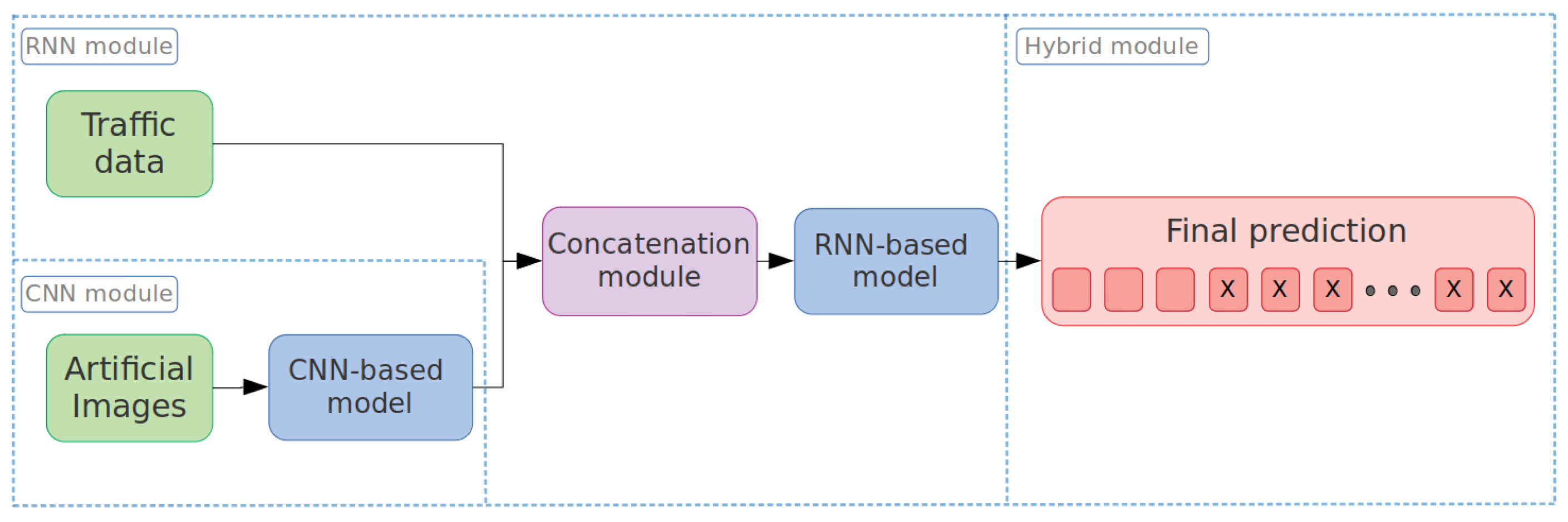
The second hybrid model architecture can be seen in
Figure 9. The
CNN-based model is used to extract the main features from the images, then they are concatenated with the scalar variables, and the final input sample is processed by the
RNN-based model to obtain the final prediction.
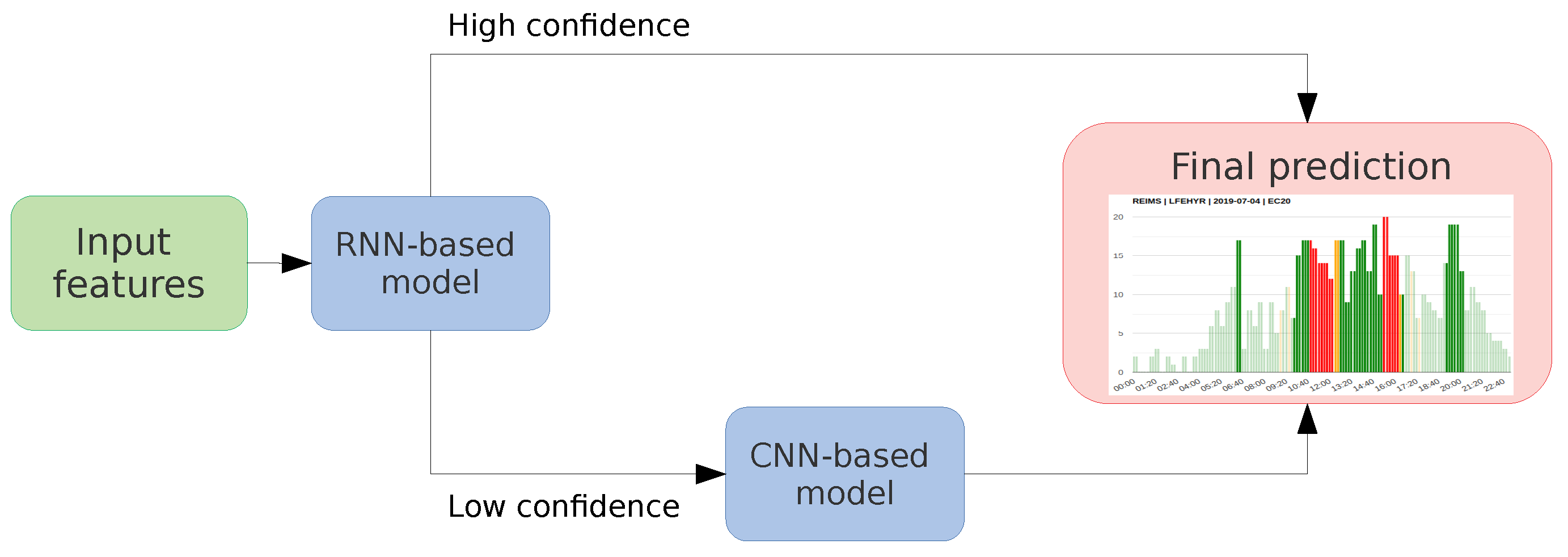
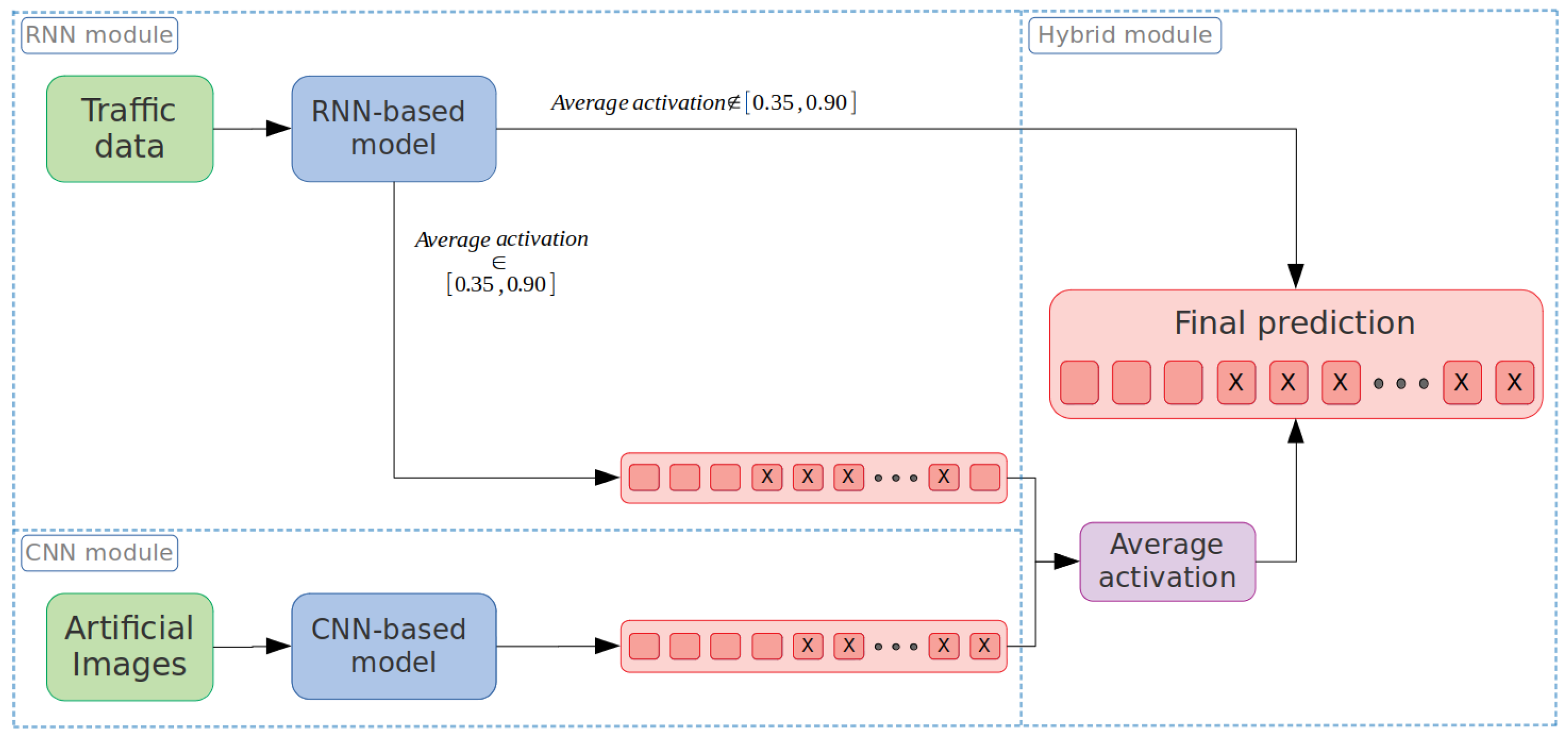
Finally, the third hybrid model architecture is based on a
RNN-CNN cascade architecture. It starts making predictions on a 30 min interval using the
RNN-based model. If the model has a high confidence-level on the prediction, it will be the final prediction. On the other hand, if the model presents a low confidence-level, it uses the
CNN-based model to refine the initial prediction (see
Figure 10). More precisely, and taking into account the information obtained from the
confidence-level analysis (see
Section 5.1), the CNN is used when the average activation from the RNN is between 0.35 and 0.90. Then, the activation values at the output layer from both models are averaged and used to obtain the final prediction. Otherwise, the final prediction only comes from the RNN model.
The reason for refining the prediction with an average activation between 0.35 and 0.90 is because we want to refine the predictions with a low confidence-level. Correctly predicted no-regulated intervals have an activation close to zero, and correctly predicted regulated intervals have an activation higher than 0.90. Therefore, using the proposed interval, we can re-evaluate intervals where the RNN is not very confident about a possible required regulation, such as intervals containing transitions (from non-regulated to regulated time-steps, and vice versa).
Notice that predicting each interval with the two models considerably increases the computational time. The predictions from the CNN are more computationally expensive (about ten times slower than the RNN), mainly due to the cost of generating the artificial images and the complexity of the network.
4. Experimental Results
In this section, we present the data used for the study, the evaluation metrics, and the results obtained over both the MAUC and REIMS regions.
Regarding the results, we present, first, the results for the RNN-based model; second, for the CNN-based model; and third, a comparison of the performance of the three hybrid models, and the extended results for the best RNN-CNN cascade model. For each model, results from the three-most regulated TVs in each region are presented together with a model able to identify regulations over the entire region, showing their flexibility and adaptability. The reason for only showing results for the three-most regulated TVs is because we have to guarantee enough instances in the TV to have sufficient variety in the samples during the training. Therefore, when possible, the idea is to use the specialized model, that is a model trained only with samples from a particular TV. However, if the specialized model is not available, the generic model trained with samples from the entire region could be used.
4.1. Dataset
For this work, we have used the AIRACs of June, July, August, and September 2019. That is 112 days (28 per AIRAC). The traffic information used to extract the scalar variables and generate the artificial images comes from the
M1 traffic, also known as the Filed Tactical Flight Model (FTFM), which is the last filed flight plan from the airline. The samples have been labeled according to the ATFM regulations cataloged as C-ATC Capacity.
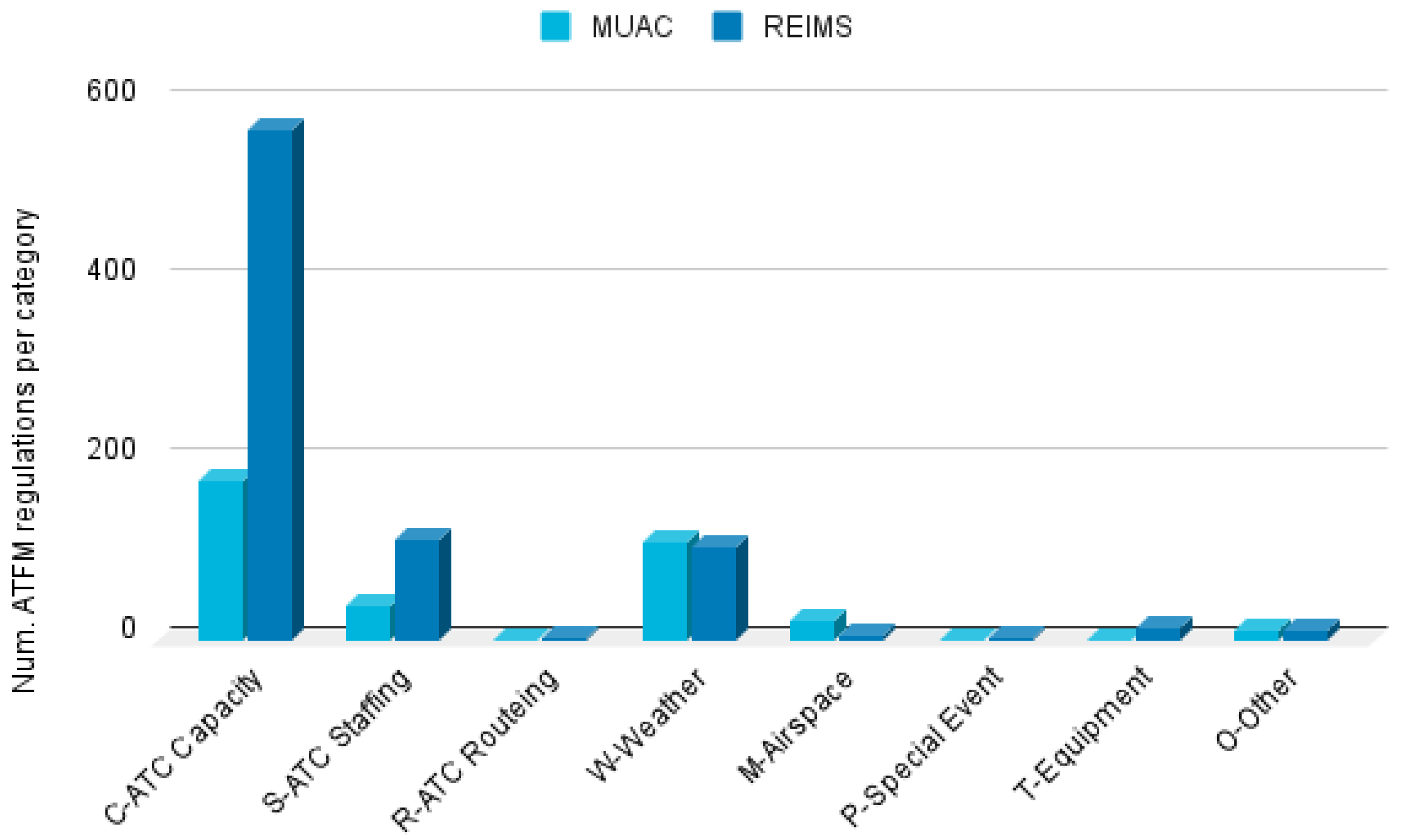
Figure 11 shows the number of instances per region and type.
For the MUAC region, we have 176 C-ATC Capacity ATFM regulations for en-route traffic along 71 different days, a mean number of regulated TVs per day equal to 2.5, and a mean duration per regulation of 122.02 min. On the other hand, for the REIMS region we have 570 regulations for en-route traffic in 96 days, a mean number of regulated TVs per day equal to 5.96, and a mean duration of 101.2 min.
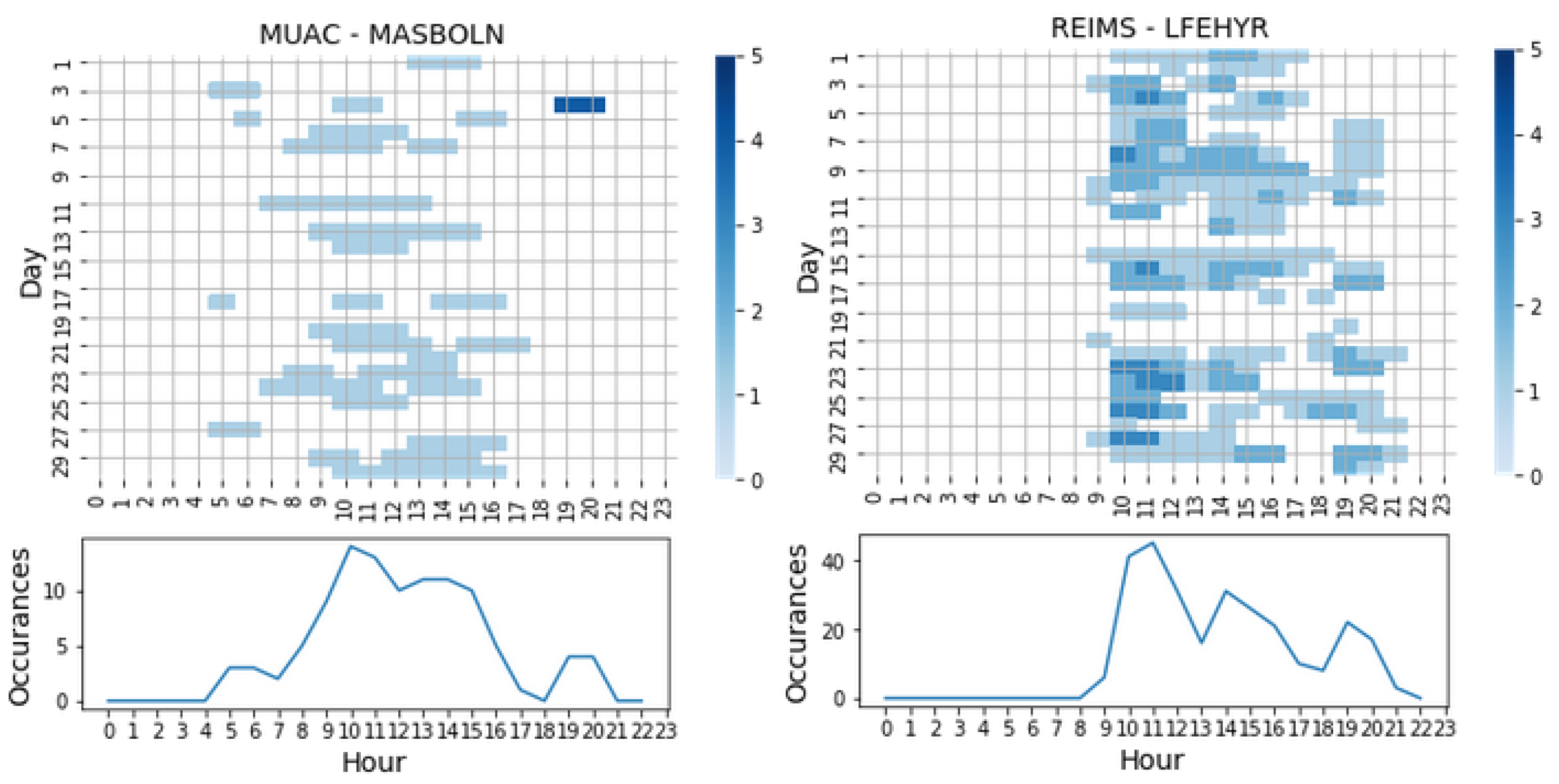
As an example,
Figure 12 shows the regulations for the most regulated TV in the MUAC and REIMS regions along the four months of data we have. The regulations from the four months have been stacked and used the color map to show coincidences between days and hours. As can be seen, most of the regulations were implemented between 10 a.m. and 11 a.m., but they also appear in all the open hours. Notice that similar characteristics can be seen in the other TVs of both regions.
Regarding the input samples, the 30 min intervals can contain time-steps of three types: non-regulated from days without regulations, non-regulated from days with regulations, and regulated from days with regulations. For instance, if there was a regulation from 10:00 a.m. to 11:00 a.m., and the input sample covers the interval from 9:45 a.m. to 10:15 a.m., the framework will show a positive label for the time-steps inside the regulated period (from 10:00 a.m. to 10:15 a.m.). Moreover, we decided to use a balanced dataset formed by approximately the same number of positive and negative time-steps (half of the negative samples were extracted from days without regulations and half of them from days with regulations) to help the model precisely identify the moment a regulation starts and ends.
Finally, to ensure that samples in the training set are not used for the testing, from the four available AIRACs, the first three (84 days) are used for training and the fourth (28 days) for testing (conventional 70–30% split). In the end, the dataset used consists of approximately 1500 30 min intervals for the MUAC region and 5000 30 min intervals for REIMS.
4.2. Evaluation Metrics
This subsection describes the metrics used to quantify the performance of the presented models. The models are evaluated at two levels of granularity, depending on whether the predictions are made at the
time-step level or at the
interval level (see
Section 3.2).
In both cases, the following classification metrics have been computed:
Accuracy: Ratio of correct predictions (both positives and negatives).
Recall: Ratio of actual positives that were correctly predicted.
Precision: Ratio of positive predictions that were correct.
F1 score: Harmonic mean of the precision and recall.
where True Positive (TP) refers to correct positive predictions, True Negative (TN) refers to correct negative predictions, False Positive (FP) refers to wrong positive predictions, and False Negative (FN) refers to wrong negative predictions.
4.3. RNN-Based Model Performance
Table 1 summarizes the results obtained using the
RNN-based model over the three-most regulated TVs in both the MUAC and the REIMS regions. The results obtained using a single model for the whole region are also included.
From the time-step classification results, it can be seen that the specialized models exhibit a better overall performance than the models for the entire regions. If we focus on the specialized models, we can see accuracy and recall higher than 80% for all the TVs, and precision between 70% and 90%. In the best case of the MUAC region (BOLN), the model achieves an accuracy of 90.95%, a recall equal to 98.11%, and a precision of 85.51%. The extremely high recall value indicates that nearly all the regulations in this TV are being detected. In the worst scenario (B3EH), an accuracy of 84.14%, recall equal to 92.98%, and precision equal to 70.51% are obtained. The low precision makes this TV worse than D6WH, where an F1-score of 81.75% is obtained, versus the 80.82% in B3EH. On the other hand, the best scenario for the REIMS region (LFE5R) exhibits an accuracy equal to 92.46%, a recall equal to 88.82%, and a precision of 91.30%. In the worse scenario (LFEHYR), the accuracy, recall, and precision obtained are 80.06%, 80.31%, and 80.25%, respectively.
When the predictions are done at the interval level, all individual TVs in the MUAC region improve all the metrics. However, for the model working over the whole region, despite the improvement in both the accuracy and recall, it presents a 3% drop in the precision (78.57% vs. 75.87%). This is not the case for the REIMS region where the Interval analysis improves the overall performance in all the scenarios. Nonetheless, the important aspect to extract from this second analysis is the fact that all the models exhibit a recall equal to 100%. Therefore, they were able to detect all the 30 min intervals that contained a regulation.
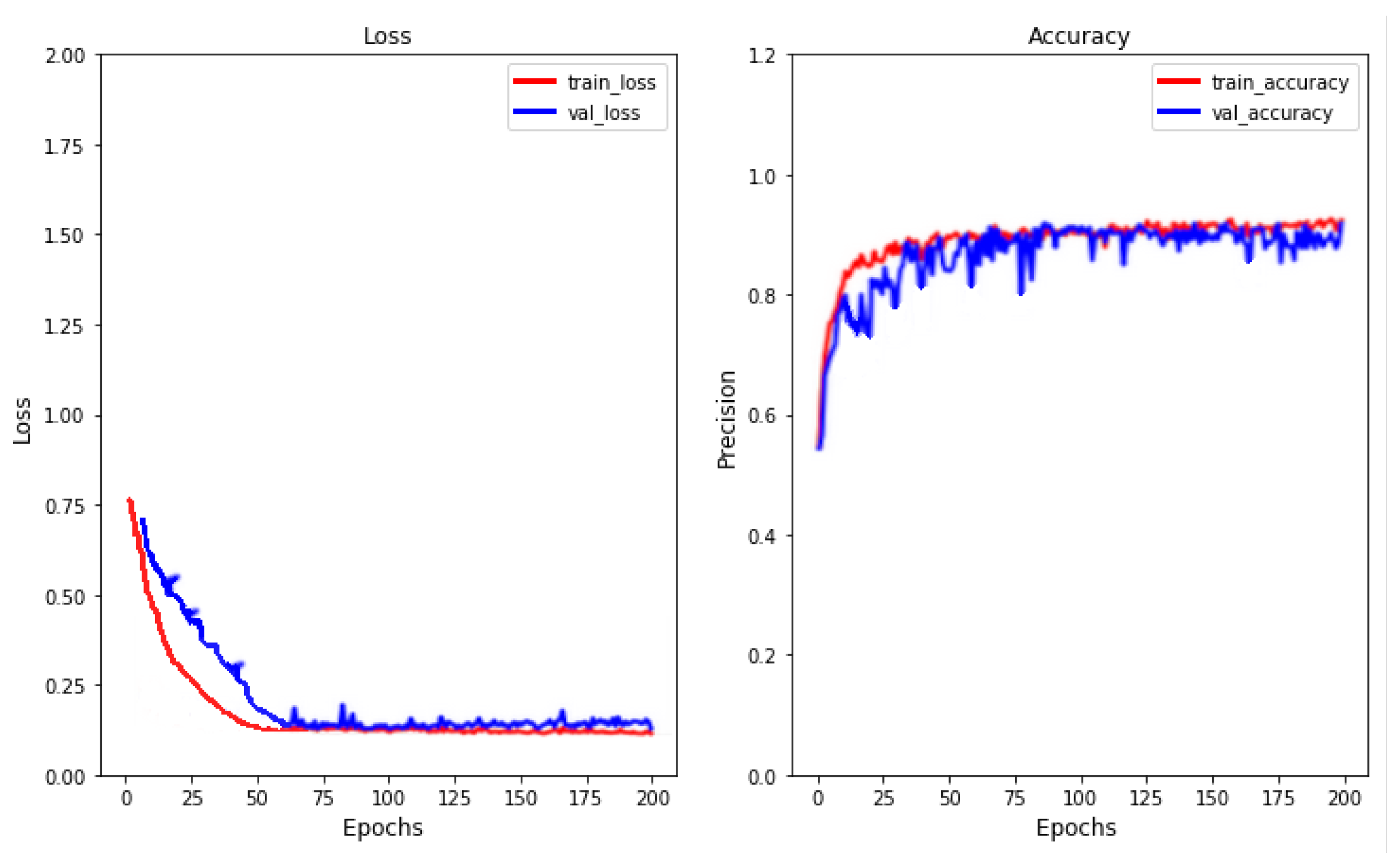
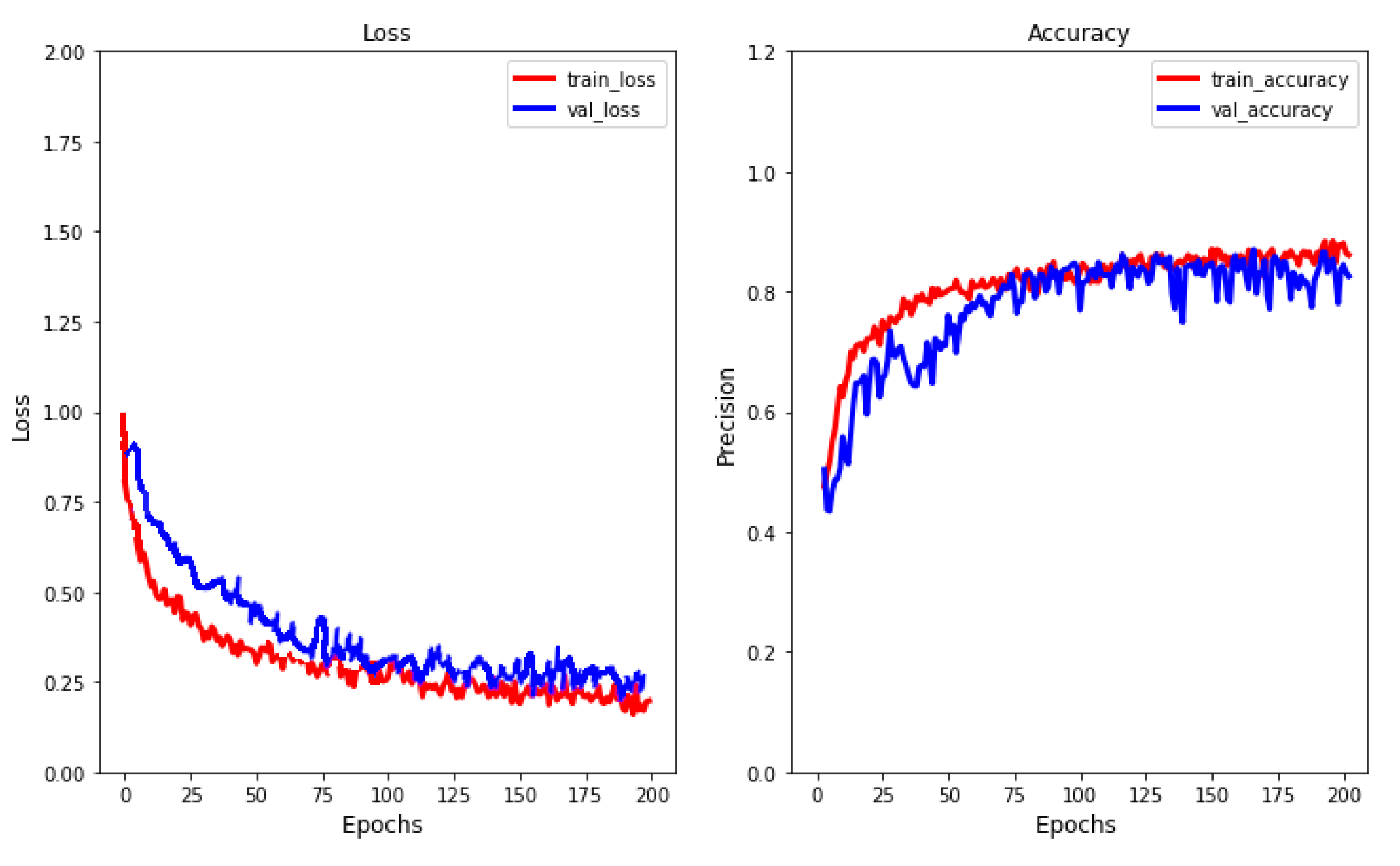
Last, but not least, as an example, to show the proper behavior of the models,
Figure 13 shows the learning curve reported by the
RNN-based model used to detect ATFM regulation for the TV MASBOLN in the MUAC region. We decided to present the behavior of the model in this scenario because (a) MUAC is an intermediate region in respect to the number of regulations available, and (b) MASBOLN is the most regulated TV in this region, and therefore, a challenging TV. Therefore, it is a good representation of the scenarios studied in this work.
As it can be seen, the model does not present underfitting. However, there is some overfitting at the end of the training (from epochs 140 to 200). Moreover, some noisy movements can be seen around the validation loss, indicating that the validation dataset is not representative enough of the model’s generalization ability. These two drawbacks come from the limited number of samples we have available for the training/testing. Nevertheless, the results obtained indicate that the model is working properly, and these issues can be solved, extending the datasets when more data is available.
4.4. CNN-Based Model Performance
Table 2 shows the results obtained with the
CNN-based model. For the
time-step classification, the specialized models also present better performance than the models for the entire regions. For the MUAC region, the specialized models reported at least an 82% F1-Score, while the model for the entire region exhibits an F1-Score equal to 80.41%. This is also the case for the REIMS region, with at least an F1-Score of 82% in the specialized models, and an F1-Score of 81.45% for the entire region. If we analyze the accuracy, recall, and precision, it can be seen that, for the MUAC region, the best model (BOLN) reported 81.65%, 85.34%, and 82.35%, respectively, while the worse model showed 78.37%, 79.53%, and 82.14%. On the other hand, for the REIMS regions, the best-specialized model reported accuracy, recall, and precision equal to 81.23%, 84.54%, and 85.63%, respectively, while the worse scenario showed 83.57%, 84.23%, and 81.45%.
On the other hand, the interval classification presents a higher performance for all the studied TVs across regions. For the MUAC region, a consistent improvement can be seen for the specialized models with an increase up to 5% in the F1-Score (BOLN). A similar improvement is obtained in the model for the entire region, where the MUAC region exhibits the biggest improvement with a 5% increase in the accuracy, and up to 14% in the recall. However, it presents a drop of 4% in the precision. For the REIMS region, the improvement in the results is also consistent across TVs. Nonetheless, we can see that less regulated intervals are detected in REIMS than in MUAC (recall around 85% VS recall around 88%).
Finally, to show the correct behavior of the models,
Figure 14 shows the learning curve reported by the
CNN-based model used to detect ATFM regulation for the TV MASBOLN in the MUAC region (same as for the
RNN-based model in
Section 4.3).
The CNN-based model exhibits a slightly less high performance than the RNN-based model, the reason why its loss is also higher. Furthermore, some noisy movements can be seen around both the training and validation losses, indicating the under-representation of the samples used. However, the model does not present underfitting or overfitting in the training nor in the validation. Therefore, these issues can be mitigated, extending the datasets when available. Last, but not least, the CNN-based model exhibits a downtrend in the training loss, indicating the performance could improve using a larger training dataset.
4.5. RNN-CNN Hybrid Model Performance
Finally, we present the results for the three hybrid models that use the previous RNN-based model and CNN-based model. First, a general comparison between the three model’s performance. Second, an extended analysis of the best hybrid model, the RNN-CNN cascade model.
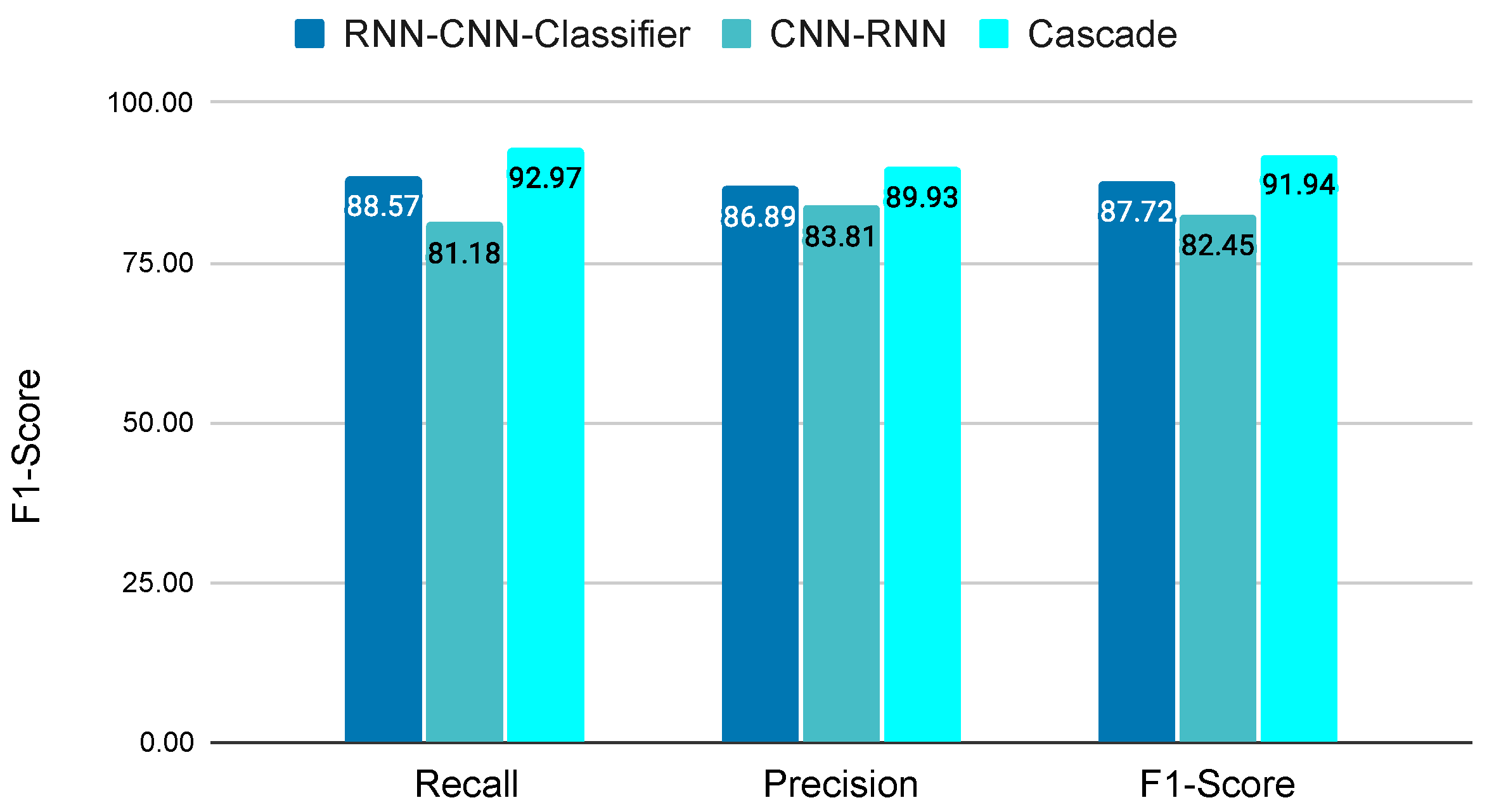
Figure 15 shows the average recall, precision, and F1-Score reported by the three studied hybrid models.
RNN-CNN-Classifier shows the results obtained by the hybrid model that uses the
RNN-based model to process the scalar variables, then the artificial images are passed through the
CNN-based model, and finally, a third classification model is used to produce the final prediction.
CNN-RNN corresponds to the hybrid model that uses a
CNN-based model to extract the main features from the images, then they are concatenated with the scalar variables, and the final input sample is process by the
RNN-based model to obtain the final prediction.
Cascade refers to the hybrid model based on a cascade architecture.
The RNN-CNN-Classifier presents a good performance, with a higher recall than precision. Moreover, its computational time is one of the largest because the images for all the samples must be created. CNN-RNN is the hybrid model with worse performance, probably because the predominant model is the CNN-based model, which has a worse overall performance. Furthermore, it requires the creation of all artificial images. On the other hand, the RNN-CNN cascade model has the best overall performance, probably because the predominant model is the RNN-based model. Therefore, we will focus on the results of the hybrid model based on the RNN-CNN cascade architecture.
The classification metrics of the
RNN-CNN cascade model are shown in
Table 3. The
time-step classification analysis exhibits a better performance than the previous individual
RNN-based model and
CNN-based model in all the studied TVs. It is able to improve precision by up to 4% on average, which has the weakest parameter. In the best scenario (REIMS-LFE5R), it exhibits a 10% improvement.
The interval classification analysis shows that with less granularity in the predictions, the performance of the model increases. The accuracy can improve up to 9% (LFE5R from 92.93% to 98.15%), the recall can be increased up to 15% (LFEHYR from 85.28% to 100%), and the precision increments up to 4% (LFE4N from 87.48% to 91.43%). In all scenarios, this analysis improves the overall performance of both the specialized and global models across regions, with an average increment of the F1-Score equal to 5%. Moreover, the results show that all the regulations are detected because the recall is equal to 100%.
5. Model Explainability
Understanding the reason behind the predictions done by an Artificial Neural Network (ANN) is crucial to ensure compliance with company policies, industry standards, and government regulations (see [
37] for further details). Moreover, it shows stakeholders the value and accuracy of the findings.
In this article, we want to focus on explainability. That is, obtaining theoretical guarantees on the expected behavior of machine learning-based systems during operation. With that goal, two analyses are performed. First, a confidence-level analysis to show how sure the model is about the predictions it does. The larger the input “signal” to the neurons, the more confident the model is about the regulation. Second, we use a game theory approach, called SHapley Additive exPlanations (SHAP), to explain the output of the models. It compares each neuron’s activation and assigns contribution scores by optionally giving separate consideration to positive and negative contributions, and therefore identifying which input features are more relevant for the trained model.
Results from a specific TV model are going to be presented. The idea is to display a conceptual analysis of the behavior exhibited by the models. We decided to analyze the TV D6WH from the MAUC region. There are two reasons behind this decision: First, it is one of the models with worse performance, therefore, we can expect better results for the other TVs. Second, D6WH belongs to the MUAC region, which is the one with fewer training samples. Remember, the success of the DL models mainly depends on the quality and quantity of the input data. These two reasons make D6WH one of the most interesting sectors for the study. Similar results have been obtained for the other TVs, independently of the region.
5.1. Confidence-Level Analysis
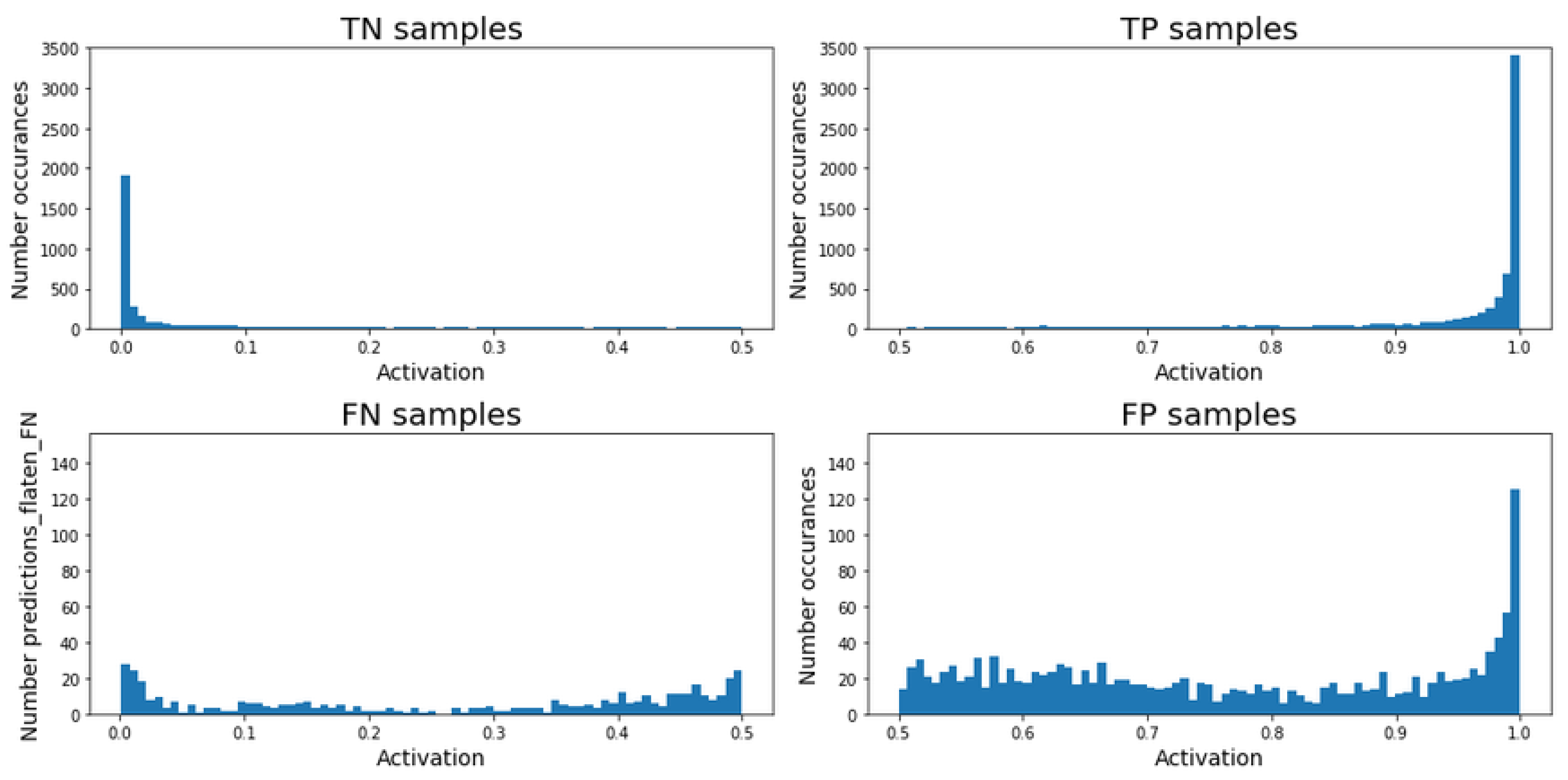
The
RNN-based model (see
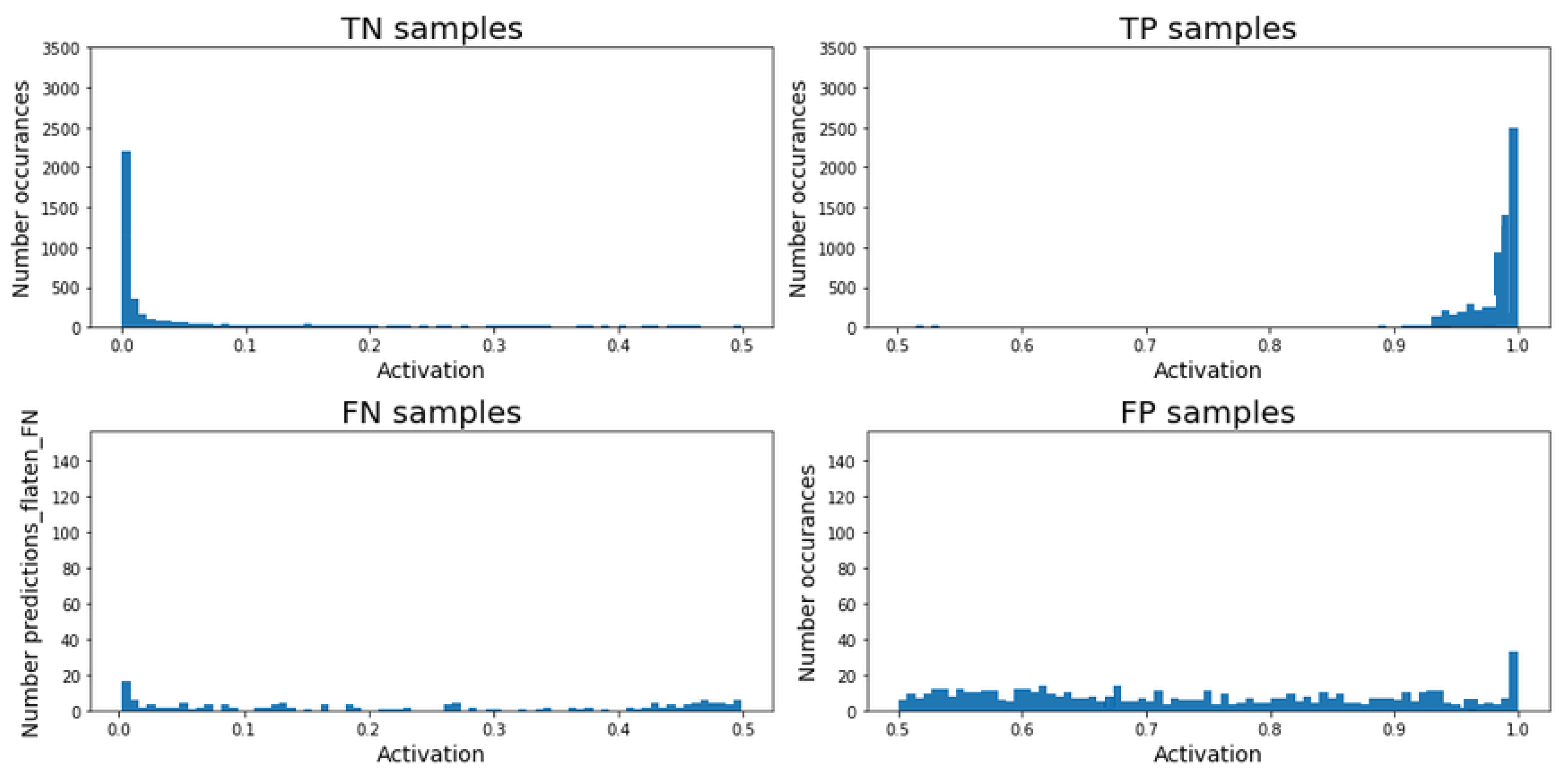
Figure 16) is able to clearly detect the TN time-steps (activation lower than 0.5), showing a small tail between 0 and 0.1. For the TP cases, the behavior is very similar, presenting a small tail between 0.9 and 1, but having the largest grouping close to 1. On the other hand, there is a small accumulation around zero and 0.5 for the FN cases. The accumulation around zero indicates that the model cataloged some time-steps as non-regulated with high confidence, but they should be predicted as regulated. Additionally, the accumulation around 0.5 shows that for a certain amount of time-steps, the model was not sure about being required a regulation or not. For the FP cases, it can be seen a larger accumulation between 0.5 and 0.7 than from 0.7 to 0.9. This indicates that, despite the considerable number of FP reported by the model, in most of the cases, it was not very confident about the prediction. Finally, as can be expected, there is a considerable accumulation between 0.9 and 1, where the model incorrectly predicted a regulation with high confidence. Nonetheless, it is important to notice that the occurrences of the FN prediction are smaller than the ones for the FP cases, indicating that the model is more likely to predict a regulation.
The
Confidence-level analysis for the
CNN-based model can be seen in
Figure 17. For the FN cases, the model presents a tail between 0 and 0.1, with an accumulation of values close to zero, and the TP cases present a tail between 0.85 and 1. On the other hand, a continuous pattern of behavior can be seen for the FN predictions, with an average value of occurrences under 20. Finally, the FP cases also show a consistent pattern of behavior across activation values between 0.5 and 0.95, and it presents a peak between 0.95 and 1. Nevertheless, the number of both FN and FP are smaller compared with the TN and TP cases.
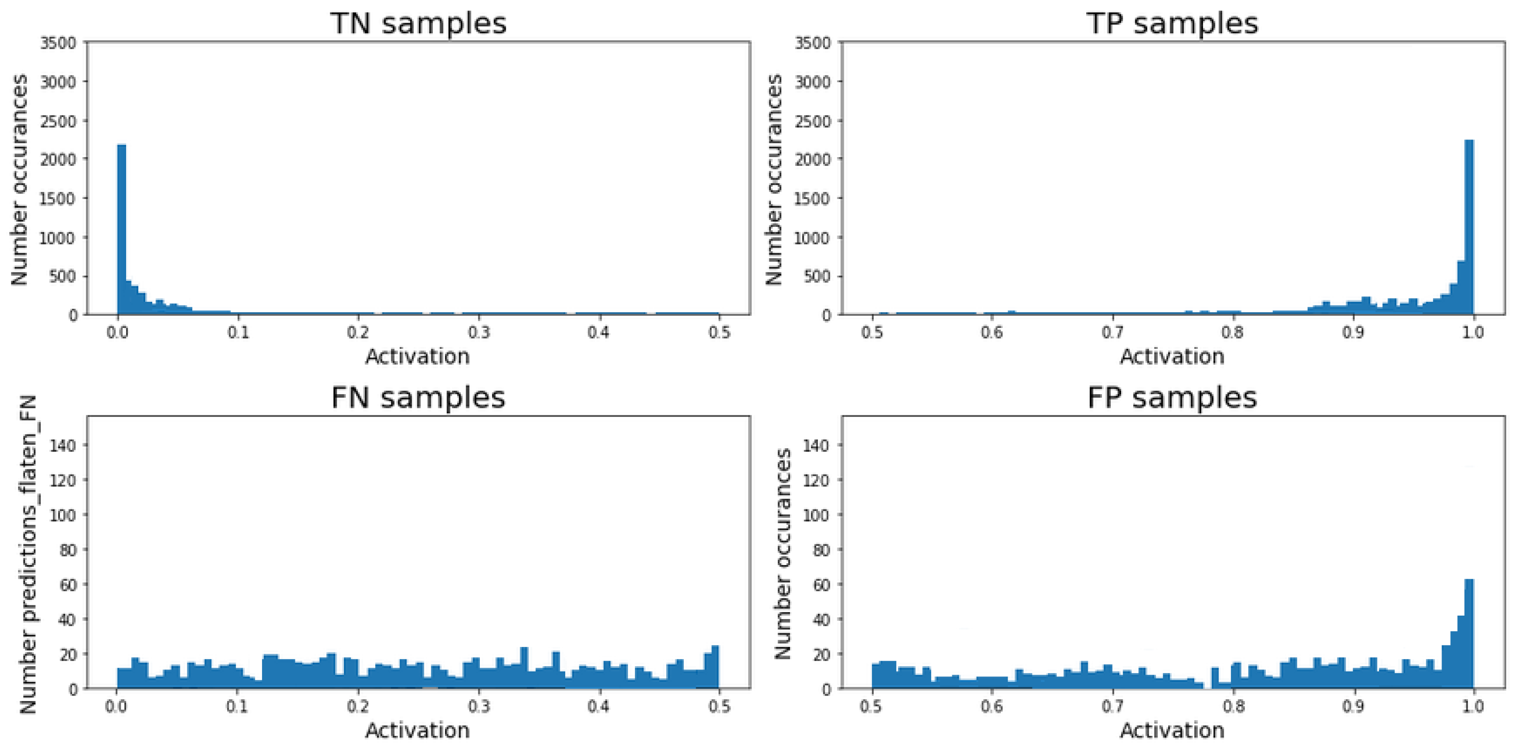
Finally, the results for the
RNN-CNN cascade model (see
Figure 18) exhibit the largest accumulation of TN around zero, with a tail between 0 and 0.1. Regarding the TP predictions, the model presents the largest accumulation between 0.9 and 1. Note that for the rest of the possible values, there are almost no occurrences. On the other hand, it can be seen that only a few occurrences are cataloged as FN cases, and therefore, the majority of regulated time-steps are identified by the model. If we analyze the FP cases, there are around ten occurrences across all the possible activation values, with a slightly higher peak close to 1.
If we now numerically compare the results between the RNN-based model and the RNN-CNN cascade model, we can see a reduction of 4.3% for the false-negative predictions (from 8.4% to 4.1%) and a 21.2% for the false-positive cases (from 39.2% to 18%). Therefore, the RNN-CNN cascade model presents higher confidence in the predictions, and it reduces the mistakes.
5.2. Shap Analysis
ANNs (aka. NNs) are collections of connected artificial neurons (nodes), where each connection (edges) can transmit a “signal” between neurons. The “signal” at a connection is a real number, and the output of each neuron is computed by a non-linear function of the sum of its inputs. The larger the sum of inputs, the higher the activation, and therefore the neuron is more likely to fire. The SHAP analysis compares the neurons’ activation and assigns positive and negative contributions scores to the different input features, depending on how relevant they are for the trained model.
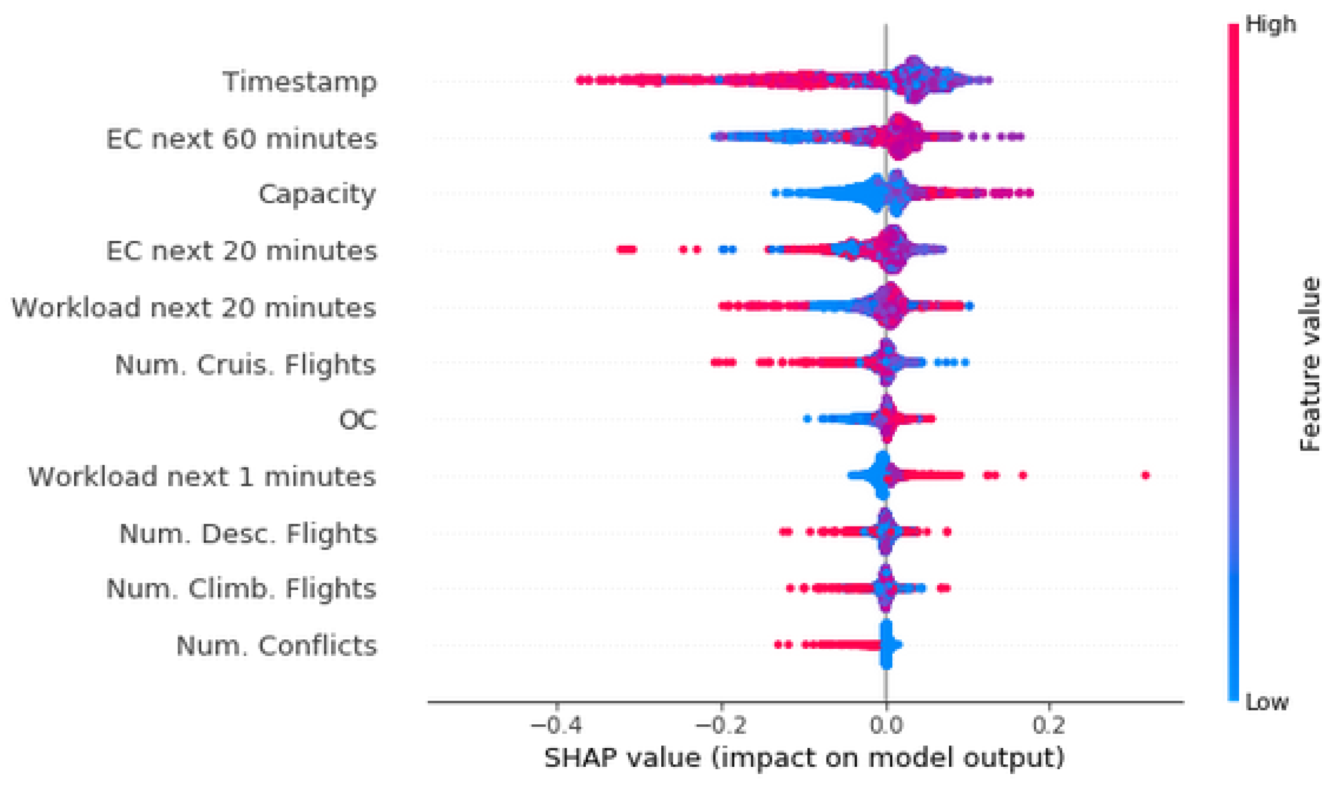
Figure 19 shows the SHAP values for the
RNN-based model. For this type of ANN, SHAP can process all the testing examples and compute the SHAP values according to their contributions.
The analysis presents the Timestamp feature as the most relevant, where samples with a smaller Timestamp (early hours of the day) are more likely to contain a regulation. The second most relevant feature is the Entry Count for the next 60 min, where larger values produce a higher activation. Therefore, if a larger number of aircraft are entering the sector, the complexity will increase, and probably a regulation could be required. This is also the case for the Capacity, larger values produce a higher activation. The higher the capacity, the larger the sector, and therefore, more aircraft being more likely to generate an overload. The fourth and fifth most relevant features are the Entry Count for the next 20 min and Expected workload for the next 20 min, which do not present a clear pattern of behavior. The reason could be that they are relevant features but in combination with another. From Number of cruising flights it can be seen that small values produce a higher activation. The Occupancy Count and the Workload for the next minute show the opposite trend. The Number of descending flights and the Number of Climbing flights do not present a clear behavior, which is surprising, because flights in these two phases should be relevant. The fact that the model cannot properly process these features could be a reason why this TV has worse performance. This is also the case for the Number of conflicts, where larger values are creating a smaller activation.
If we move to the SHAP analysis for the
CNN-based model, results similar to
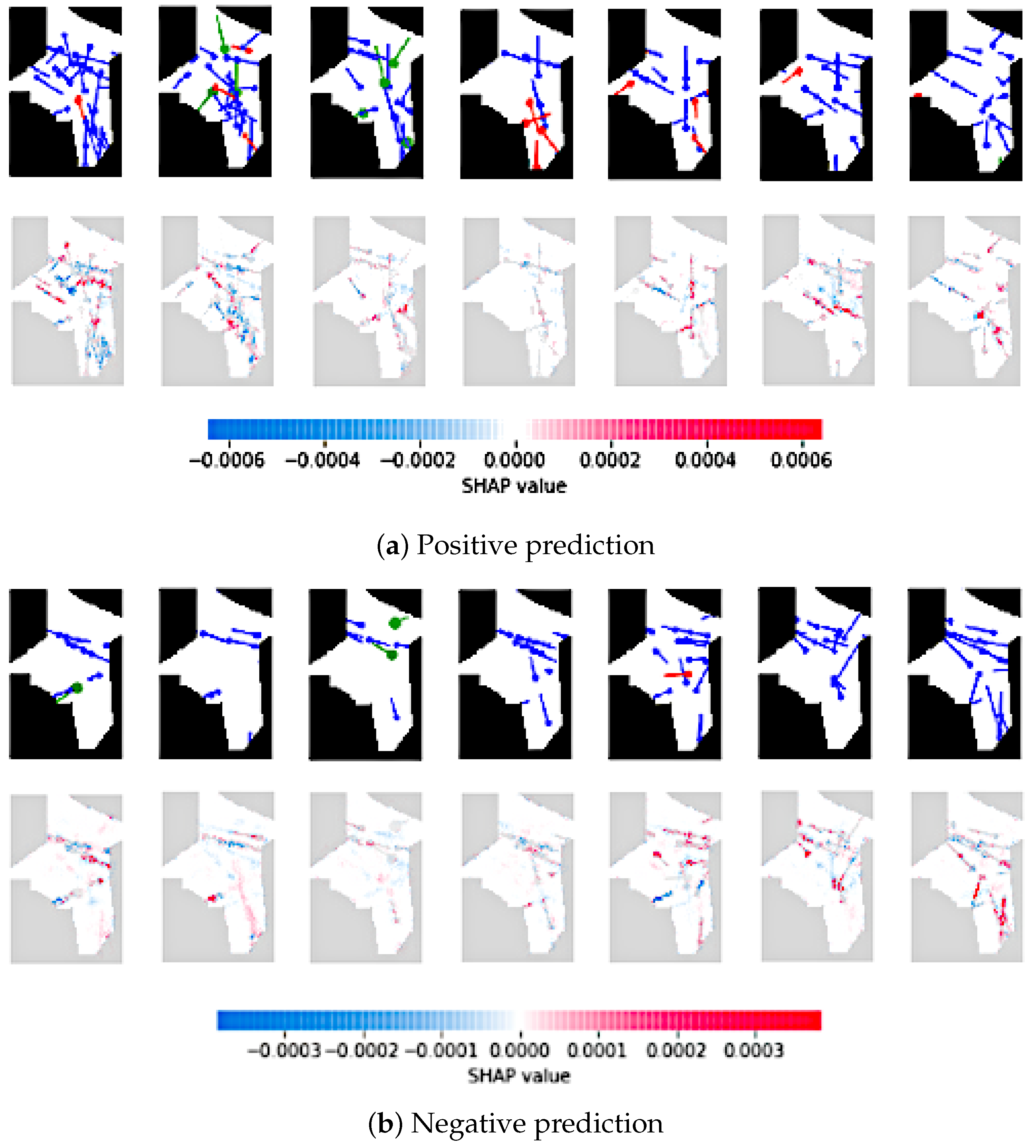
Figure 20a,b can be obtained. For this type of ANN, the SHAP analysis exhibits what elements/parts, in each input image, produce a higher activation. Therefore, it will highlight what parts of the image are more relevant when identifying regulations.
Figure 20 presents the SHAP values for a true-positive prediction and a true-negative prediction. For clearness, only one picture every five min (instead of every minute) are showed. In the case of the positive prediction (
Figure 20a), it can be observed that a considerable number of aircraft cross the images, creating a larger activation of those flights close in space with the same heading, or flights relatively close in space but with perpendicular headings. It is also interesting to see that the other main source of activation comes from flights close to the border of the TV (see the sixth and seventh images), indicating that flights entering or exiting the TV are more relevant to identify possible regulation.
On the other hand, in the case of the negative prediction (
Figure 20b), it is interesting to see a similar pattern of behavior, where aircraft close in space or entering/exiting the TV are producing a higher activation. However, this activation is lower, with a Maximum SHAP value of 0.0003. Nevertheless, the model seems to pay attention to the interaction in the two main flows of the TV: one horizontal, in the top part of the TV, and another from the top-left to the bottom-right corners. If we analyze the second image, the top flow indicates that it is not required a regulation, however, the model is presenting a higher activation for the diagonal flow. This could indicate that, even though currently there is no traffic, it is probably expected an increment, reason why it can be seen a “red line” without being any aircraft at the moment.
6. Discussion
In the current DCB process, deciding whether or not an ATFM regulation is needed in case of imbalance (prior to deciding what action to take) is a time-consuming task. Furthermore, it often depends mainly on the previous knowledge and skills of the FMP. Despite the variety of tools and metrics used, ATFM regulations continue being responsible for most of the delays and, consequently, cost. For this reason, many researchers and projects, such as the SESAR 2020 Exploratory Research program, are investigating how to overcome these limitations. However, according to the literature, most of the efforts have focused on the resolution of such imbalances, and less attention has received in the detection process. This makes it impossible to compare the performance of the presented models against other approaches, due to the lack of numerical results.
Our goal is to provide a support tool that aids the person in charge to focus quickly on the cases that deserve FMP’s attention, thus reducing the workload. Currently, all situations where demand exceeds capacity have to be studied. However, not all these cases leads to an ATFM regulation (for instance, the overload can sometimes be assumed due to its short period). The presented framework can help to considerably reduce the cases that deserve the FMPs’ attention; thus reducing the number of false-positive imbalances, and consequently, reducing the ATCO’s workload. However, due to the relatively small size of the used dataset, the framework should be trained with a larger dataset and be tested in real-world conditions to ensure its viability.
Another important characteristic of the presented system is the fact that it contains model explainability tools (SHAP analysis), which could be used to provide additional information to the person in charge, together with the predictions itself. For instance, the SHAP values from the CNN-based model can show what elements are causing the system to predict a required ATFM regulation. Nevertheless, the way of visualization to figure out the best approach should be discussed with the people in charge of the DCB process.
Regarding the results, they are consistent across different studies and regions. In the Time-step classification, it has been seen that the CNN-based model performs slightly worse than the RNN-based model. For the specialized models, the CNN-based model exhibits an average F1-Score equal to 83% while for the RNN-based model it is equal to 86%. This drop in the performance is especially significant in the accuracy and recall. However, the CNN-based model exhibits an increment between 3% and 10% in the precision for most of the models (especially in the weakest ones). The proposed RNN-CNN cascade model benefits from the best of each of the previous models. It reports accuracy between 85% and 93% for the specialized models, recall higher than 90% (except for the LFEHYR from the REIMS region with a recall equal to 85%), and precision between 81% and 94%. In other words, the RNN-CNN cascade model exhibits a higher accuracy, recall, and precision than previous models in all TVs. Notice that, for better performance, it is recommended to use specialized models trained for each particular TV. As an alternative, generic models can handle the entire regions.
For the Interval classification, we can see a similar pattern of behavior. The CNN-based model exhibits an overall slightly worse performance than the RNN-based model, and the RNN-CNN cascade model exhibits the best results. Nonetheless, the most significant result is the fact that the CNN-based model is not able to identify all the 30 min regulated. A recall between 80% and 90% is obtained while the RNN-based model and the RNN-CNN cascade model are able to identify all the regulated intervals. Therefore, the final framework can detect all the intervals that contained a regulation.
Last, but not least, the Model explainability analysis exposes a behavior close to the current CDM procedure. The confidence-level analysis shows that the RNN-CNN cascade model has 4.3% less false-negative and 21.2% less false-positive predictions than the RNN-based model. The SHAP analysis has shown that the expected incoming traffic, in combination with the capacity of the TV and the current occupancy, are key aspects to be considered when predicting C-ATC Capacity ATFM regulations. Moreover, aircraft close in space are prioritized, together with aircraft entering or exiting the TV. The transfer of aircraft is one of the main reasons for demand–capacity imbalances due to its complexity.
The obtained results validate the assumption that the selected input features are highly correlated with the target, as the models are able to generalize and correctly predict new samples. However, given the complexity of the problem, additional input features could be considered in future works to improve performance. One significant fact to consider are the collateral effects of actions carried out in the nearby pltv.
Finally, even though the framework has been developed and studied to automatically predict C-ATC Capacity ATFM regulations during the pre-tactical phase, we are confident it could also be used to detect hotspots in the tactical phase. The tactical phase is closer to D0, and consequently, there should be less uncertainty in the information. Currently, the main limitation to this end is the lack of labeled data to train the models.
7. Conclusions
We have presented and evaluated a hybrid
RNN-CNN cascade architecture to predict C-ATC Capacity regulations for en-route traffic. It uses a
RNN-based model to obtain an initial prediction of possible required regulations, and then, depending on the confidence in the prediction, it uses a
CNN-based model to refine the prediction. Moreover, it has been shown that the presented framework can be used independently of the ATC center, being a DL model that could be deployed across Europe. With this aim, we presented two analyses for model explainability, which clearly show that the model could be used in operational conditions due to the close behavior to the current procedures. However, there are still significant metrics that need to be studied to ensure the approval of
Level 1 AI applications (assistance to human) [
38].


