Article

Stealthy Configuration Optimization Design and RCS Characteristics Study of Microsatellite

College of Astronautics, Nanjing University of Aeronautics and Astronautics, Nanjing 211106, China
*
Author to whom correspondence should be addressed.
Aerospace 2022, 9(12), 815; https://doi.org/10.3390/aerospace9120815
Submission received: 24 October 2022 / Revised: 23 November 2022 / Accepted: 8 December 2022 / Published: 12 December 2022

Abstract

:
Firstly, the radar cross section (RCS) test results of the stealthy microsatellite of TianXun-1(TX-1) in the anechoic chamber are compared with the RCS numerically simulated by the physical optics method, and the accuracy of the physical optical method is verified. On this basis, in order to improve the radar stealth performance of the microsatellite, a satellite stealth configuration optimization design method is proposed with the multi-prismatic stealth configuration of TX-1 as the initial configuration, and two olive stealth satellite configurations are obtained. By comparing the RCS simulation and radar detection probability of the optimized Olive-A and Olive-B satellite stealth configurations in multiple directions, it is demonstrated that the stealth performance of the Olive-B configuration is better. Finally, the anechoic chamber test is conducted on the metallic Olive-B model, and the test results show that the test results and simulation results of Olive-B are in good agreement, which again verifies that the stealth performance of Olive-B is better than that of TX-1 and Olive-A.

1. Introduction

With the continuous development of various space-based and ground-based detection means, the in-orbit survivability of satellites is facing serious challenges. In order to achieve low detectability of satellites and strengthen the defense capability against enemy radar detection systems, there is an urgent need to apply stealth technologies to satellites. For the different threats faced by satellites under different detection systems, satellite stealth technology can be divided into radar stealth, infrared stealth, visible light stealth, and radio frequency stealth, among which one of the main threats to satellites comes from radar, and it is especially important to design and analyze microsatellites with low radar cross section (RCS) shape [1,2,3]. Since satellite stealth technology involves state secrets, not much information is available for reference.
In 1990, the first satellite of the U.S. Misty program (Misty-1) was successfully launched. The cylindrical satellite body has a conical inflatable cover underneath; the radar waves emitted from the ground to the conical inflatable cover will be refracted to other directions so that the return energy is greatly suppressed [4], and it is also the world’s first stealth satellite operating in orbit. In 2011, based on the idea of multi-prismatic design, Zheng, K. proposed three stealthy microsatellite configurations and obtained the conclusion that the stealth effect of the multi-prismatic cone is better through RCS comparison simulation [5]. In 2015, Chung, S.S.M. referred to the configuration design of the Misty satellite and replaced the conical inflatable cover with a metal cone to obscure the cylindrical satellite below. Then, the finite difference time domain (FDTD) algorithm was used to numerically simulate the monostatic RCS of conventional and stealthy satellites in the S-band [6]. In 2016, Chen, W. disclosed a radar-stealthy satellite in orbit, which is known as TianXun-1(TX-1). TX-1 is both the first stealth microsatellite developed by Nanjing University of Aeronautics and Astronautics and the first Chinese microsatellite with low target characteristics, which was launched into orbit on a CZ-4B launch vehicle from the Taiyuan Satellite Launch Center. The satellite has an in-orbit mass of 61 kg, an envelope size of less than 1 m, an orbital altitude of 495 km, and its specific configuration is a combination of a hexagonal column, a hexagonal platform, and a hexagonal cone [7]. In 2017, Zhu, D. proposed a satellite configuration with both radar stealth and optical stealth with a peak optical cross section (OCS) of only 0.082 m2, which is not easily identified by optical detection system surveillance [8]. In 2017, Gong, J. used a high-frequency asymptotic approach to extract the electromagnetic scattering characteristics of an optoelectronic/infrared reconnaissance satellite and obtained the scattering bright spot distribution of the satellite [9].

2. Theoretical Basis

2.1. RCS Numerical Calculation Method

From the perspective of computational electromagnetics, RCS calculation methods can be divided into differential equation methods, integral equation methods, finite element methods, and high-frequency approximation methods applicable to targets in the optical region. In the frequency range studied in the thesis, the satellite target is mainly in the optical region. The method of moments (MOM) is a typical integral method, which does not have the problem of convergence by using a direct calculation of the matrix, and the total number of unknowns is greatly reduced by using a surface grid for partitioning, but because of the coupling between the “sources”, the matrix is a dense matrix, which leads to a slow MOM calculation [10,11]. Most of them are used for RCS calculations for some fine electric small or electric medium size targets. Multilevel fast multipole method (MLFMM) uses some acceleration algorithms on the basis of MOM, which reduces the memory requirement and increases the computational speed and can be used to solve RCS of electrically large size, but the iterative solution is prone to non-convergence when encountering pathological matrices, such as aircraft intakes, tail jets, and other cavity structures. The physical optics (PO) method is mainly applied to the scattering characteristics of the target in the optical region to solve. Starting from the Stratton–Chu scattering field integral equation, and assuming that the value of the target surface current is equal to the current value when the target is an ideal smooth plane, the physical optics current is accordingly integrated to obtain the scattering field in the far region of the target [12,13].
Based on the Stratton–Chu integral equation [14,15,16,17], the electric and magnetic fields can be determined as:
E ( r ) = 1 j ω ε 4 π S [ 3 k 2 R 2 + j 3 k R R 5 e j k R R × ( R × J S ( r ) ) + 2 J S ( r ) 1 + j k R R 3 e j k R ] d S
H ( r ) = 1 4 π S 1 j k R R 3 e j k R ( r × J S ( r ) ) d S
where j   is the imaginary unit, k   is the number of free-space waves, ω   is the electromagnetic wave angular frequency, ε   is the dielectric permittivity, r is the coordinate vector of the field point, r   is the coordinate vector of the source point, S   is the area of the surface element being accumulated, and R is the distance between the field point and the source point. Based on the above assumptions of PO, the target surface current excited by the radar wave is:
J S = { 2 n × H , Z I 0 , Z D
where n is the unit vector of the target surface normal vector, Z I is the illuminated area, and Z D   is the dark area [16,18]. If the incident wave is a plane wave, then:
E i ( r ) = | E 0 | e j k r
where k is the incident electromagnetic wave vector. Then, the electric field formula can be transformed into:
E S ( r ) = k 2 j ω ε 2 π η S r ^ × { r ^ × [ ( n ^ ( r ) E 0 ) k ^ ( n ^ ( r ) k ^ ) E 0 ] } × e j k ( R + k ^ r ) R   d S
The integral term could be recorded as:
I = S r ^ × { r ^ × [ ( n ^ ( r ) E 0 ) k ^ ( n ^ ( r ) k ^ ) E 0 ] } e j k ( r ^ + k ^ ) r d S
According to the definition of radar cross section, the RCS of a single facet element is calculated as:
σ = 4 π λ 2 | I | 2
The total RCS of the target is contributed to by numerous facets, and thus the total RCS is:
σ t = | f = 1 N σ f | 2
where σ f represents the RCS of the f-th facets element.
The RCS arithmetic mean and RCS magnitude are chosen to quantify the stealth performance of the target.
σ m = max { σ i }
σ ¯ [ a , b ] = i = 1 N σ i N
where σ i is the RCS at the i-th incident angle, σ m is the RCS maximum, and σ ¯ [ a , b ] is the RCS arithmetic mean in the [a, b] angle domain.
RCS is a hypothetical area, the unit is meter squared, but the RCS fluctuation range of the target at different angles is very large, for example, the RCS fluctuation range of a stealth aircraft can easily reach six orders of magnitude, and it is difficult to clearly show the change characteristics of the target RCS in the figure. At this time, it needs to be expressed in logarithmic form:
σ dBsm = 10 lg σ m 2
In data processing, it is sometimes necessary to express RCS in units of m2, and Equation (11) can also be written as:
σ m 2 = 10 0.1 σ dBsm

2.2. Anechoic Chamber RCS Measurement Method

The target RCS is further obtained from the measured S-parameters, using the relative comparison method. Taking a standard metal sphere with a known scattering section as the reference object, the scattering section of the standard sphere is the formula   π r 2, and r is the radius of the standard sphere.
The normalized backscattering RCS of the metal calibration sphere is:
σ π r 2 = ( j k r n = 1 ( 1 ) n ( 2 n + 1 ) × [ ( k r J n ( k r ) n J n ( k r ) k r H n 1 ( k r ) n H n ( 1 ) ( k r ) ) ( J n ( k r ) H n ( 1 ) ( k r ) ) ]
H n ( 1 ) ( k r ) = J n ( k r ) + j Y n ( k r )
where r is the radius of the sphere, k = 2 π / λ , J n   is the n-order first class Bessel function, H n ( 1 ) is n-order Hankel function, and Y n is n-order second class sphere Bessel function.
Under the same measurement conditions, the ratio of the scattering power intensity of the target and the standard sphere is the ratio of the RCS of the two. The test system directly measures the transmission S-parameter of the target, which is S 21 , and its size is proportional to the scattering power of the target and RCS. Let the RCS and S 21   of the standard sphere be σ 0 and S 0 ; the RCS and S 21 of the target are σ 1 and S 1 .
σ 1 = σ 0 S 1 S 0
If σ 0   and σ 1   are in dBsm, S 0 and S 1 are in dB, then the above equation becomes:
σ 1 = σ 0 + S 1 S 0
From the above equation, the S-parameters of the standard sphere with known RCS and the target to be measured separately, as well as the RCS of the target, can be calculated.

3. Stealthy Satellite Anechoic Chamber Test Verification

In order to verify the accuracy of the physical optics method, this paper takes the TX-1 stealthy microsatellite as an arithmetic example. Firstly, the high-quality electromagnetic calculation model of TX-1 is obtained by geometric cleaning, as shown in Figure 1a. Then, the RCS results obtained by testing the satellite in the anechoic chamber are compared with the results calculated by the physical optics method [18]. The frequency of this test is set to 5.45 GHz and the polarization form is VV polarization. The relevant in-orbit parameters of TX-1 are given in Table 1.
From Figure 1b, it is easy to see that the RCS value is solved by using PO is in good agreement with the actual RCS value of the satellite obtained from the test in the anechoic chamber. Specifically, there is a clear wave peak in the symmetric angular domain from 84 to 96° centered at 90° (right at the tip of the satellite), which corresponds to the tip of TX-1. The experimental results in this angular domain are obviously higher than the simulation results because PO is the method of tangent plane approximation, which simply assumes that the surface of the accumulated target is completely smooth and flat, and directly substitutes the surface field into the integral equation, so PO does not solve the cusp scattering problem well. The mean values of RCS obtained from the simulation and experiment after removing this error-ridden angular domain are −17.86 dB and −17.96 dB, respectively, with only 0.1 dB difference between them, which proves the accuracy and feasibility of using the high-frequency asymptotic approach to solve the satellite RCS in the optical region.

4. Stealthy Configuration Optimization Design of TX-1

4.1. Optimal Design of Satellite Body

Figure 2 shows the specific ideas and methods used to optimize the stealth satellite. Firstly, the four-sided cone configuration with symmetric structure is obtained by referring to the stealth configuration of TX-1, and then the number of edges of the symmetric cone is increased to eight and ten edges, as shown in Figure 2. Finally, using the idea of limit, the number of edges is taken to be large enough to obtain the final optimized configuration (olive).
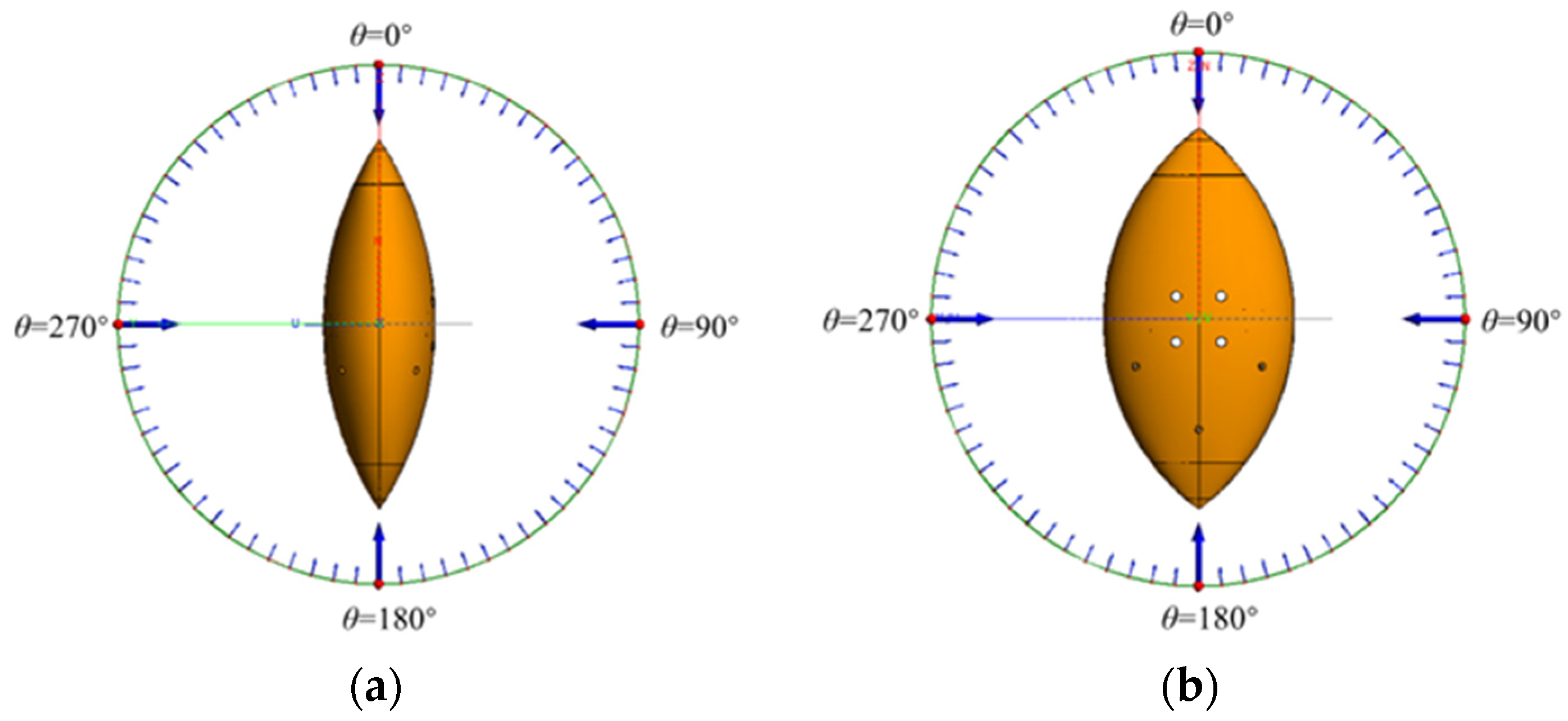
Olive-A can be divided into stealthy and non-stealthy attitudes, as shown in Figure 3. The Olive-B is a highly symmetric rotating body with the same RCS distribution curve in all directions, so it can achieve omnidirectional stealth and there is no difference between stealth and non-stealth attitudes.
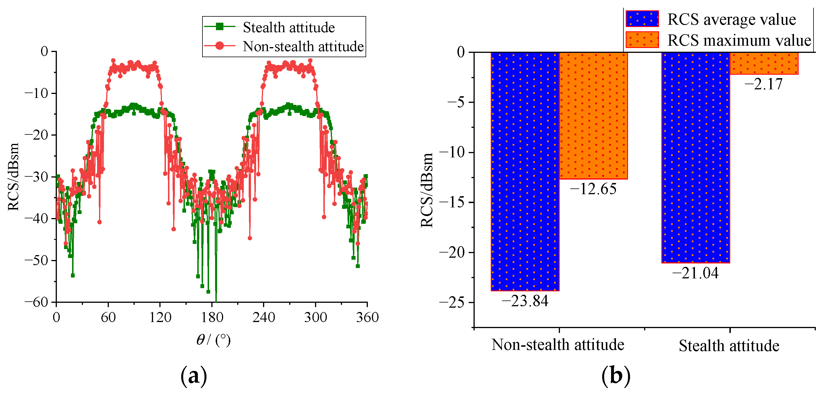
From the simulation results in Figure 4, it is easy to see that the RCS in the non-stealth attitude of the Olive configuration A is about 10 dBsm higher than that of the stealth attitude in the angular domains of 60–120° and 240–300°, while the difference in the RCS in the other angular domains is very small. In fact, the stealth performance of the satellite decreases when the incident radar wave gradually deviates from the stealth attitude and reaches the worst performance when it reaches the non-stealth attitude.
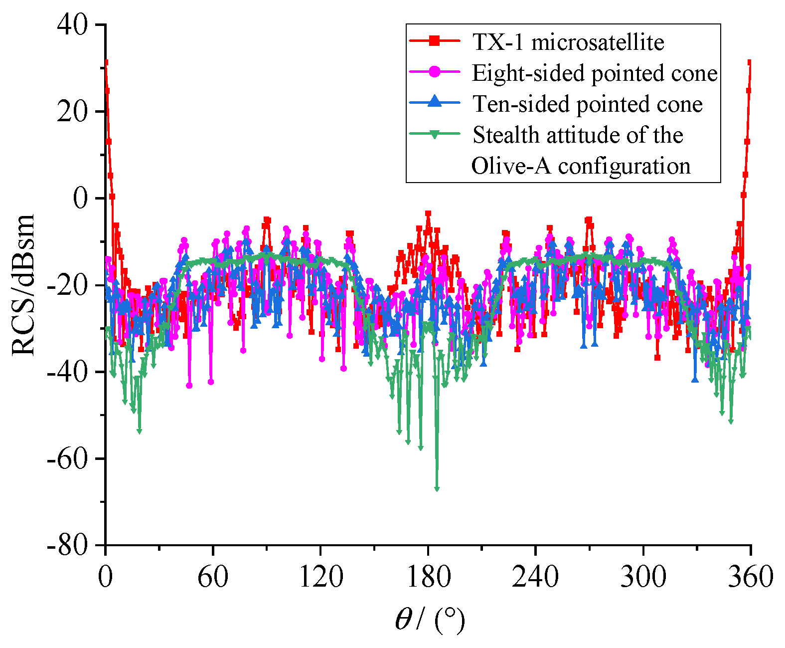
To verify the feasibility of the optimization method in Figure 2, the central frequency point of the X-band is selected to analyze TX-1, the eight-sided pointed cone, the ten-sided pointed cone, and the stealth attitude of Olive-A configuration. The comparison of the RCS numerical calculation results of the four stealth configurations at the X-band (10 GHz) is given below.
From Figure 5 and Table 2, it is easy to find that the pattern is very obvious in the X-band; the stealth performance of the four configurations is Olive > ten-sided cone > eight-sided cone > TX-1, both in terms of RCS mean and RCS maximum. The arithmetic mean and maximum values of RCS of the Olive configuration are lower than those of the TX-1 by 3.65 dB and 43.97 dB, respectively, while the RCS reduction in the ten-sided cone is better than that of the eight-sided cone. This again confirms the correctness and feasibility of the optimized design method in Figure 2. In addition, the RCS distribution of the Olive configuration is very gentle in the symmetric angular domain centered at 90° and 270°, while the RCS curves of the other three configurations oscillate strongly and have more scattering peaks, which is extremely unfavorable for the stealthy configuration design.
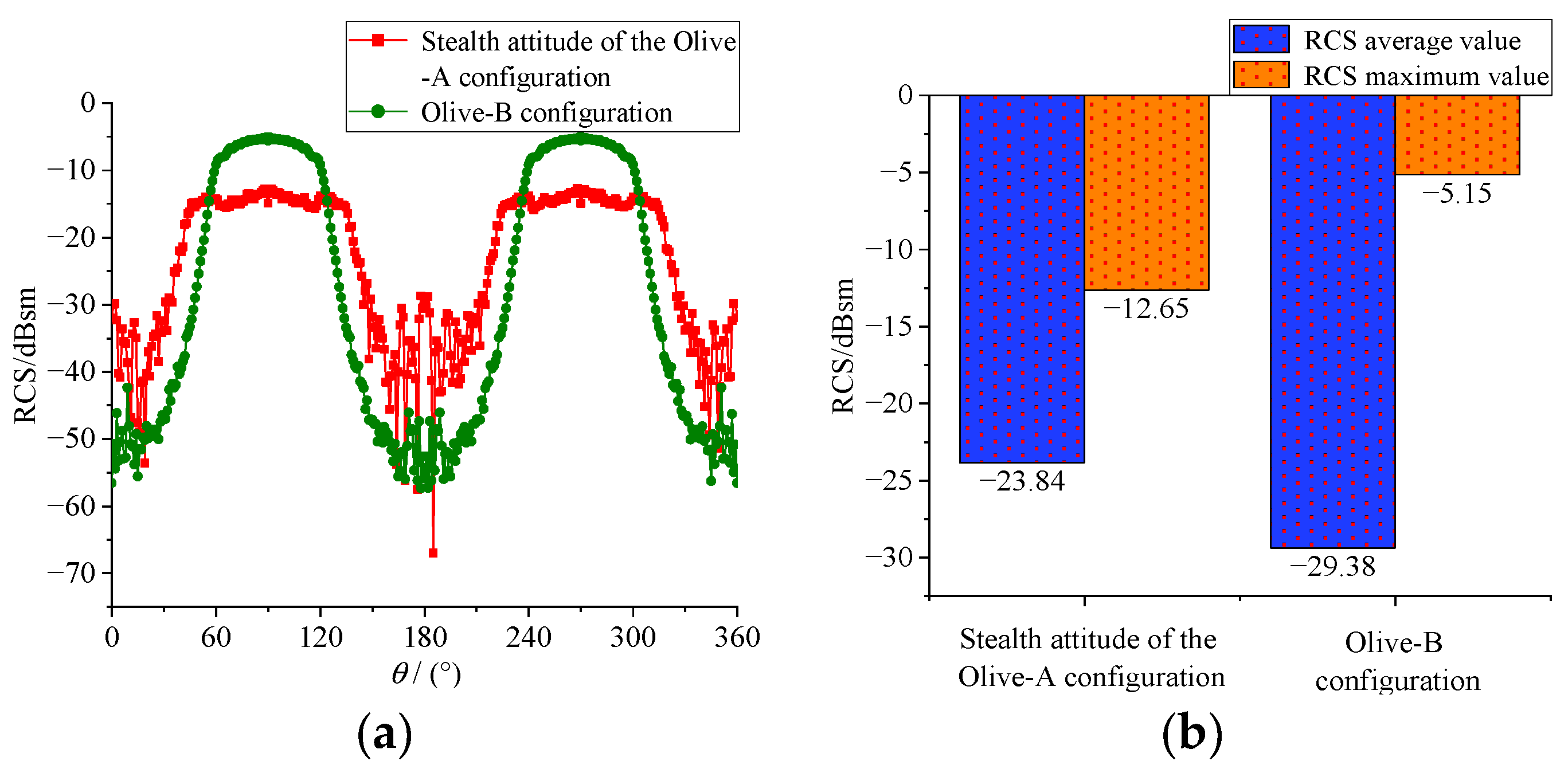
In order to be able to deal with threats from both space-based and ground-based radar detection systems when the satellite is in orbit, it is necessary to make the satellite configuration as omnidirectional as possible to achieve stealth. Although the difference between the mean RCS values in the non-stealthy and stealthy attitudes of Olive-A is small, the configuration can be further optimized to improve the omnidirectional stealth performance. The RCS comparison between the stealth attitude of Olive-A and the optimized Olive-B at 10 GHz is given in Figure 6.
From Figure 6, it can be seen that although the scattering characteristics of the two stealth configurations are relatively similar, there are some significant differences. The RCS of the Olive-B configuration is lower than the stealth attitude of the Olive-A configuration in all angular domains beyond 56 to 123° and 236 to 304°. Specifically, the RCS amplitude of the Olive-B configuration is higher than that of the stealth attitude of the Olive-A configuration, but its RCS mean value is lower than that of the stealth attitude of the Olive-A configuration by 5.54 dBsm, and the RCS mean value reduction effect is significant.
From the above analysis, it is easy to find that the RCS mean value of the stealth attitude with the best stealth effect of the Olive-A configuration is still inferior to that of the Olive-B configuration. When the incident wave gradually deviates from the stealth attitude, the RCS mean value of the Olive-A configuration will continue to increase, and the stealth performance gap between it and the Olive-B configuration will be even larger. In summary, since the omnidirectional stealth performance of the Olive-B configuration is significantly better than that of the Olive-A configuration, the Olive-A configuration is eliminated and the Olive-B configuration is determined as the final stealth configuration of the satellite.

4.2. Olive-B Configuration Satellite Anechoic Chamber Test Verification

As shown in Figure 7, this RCS test system consists of an anechoic chamber, transmitting and receiving antennas, a turntable, a vector network analyzer, a low-noise amplifier, and a target to be tested.
It should be noted that the length, width, and height in Table 3 refer to the dimensions of the Olive-B; the antenna gain and flap width vary with frequency, and the values given in Table 3 are at 10 GHz.
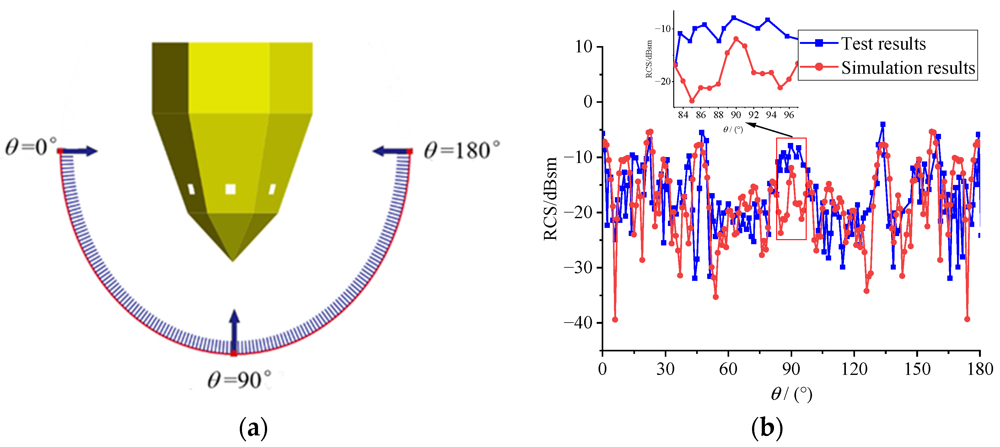
The radar band for the electromagnetic test and simulation is set to the X-band and the polarization form is VV polarization. The comparison of the test and simulation results of the anechoic chamber of the Olive satellite is given in Figure 8. It is easy to see from the figure that the simulation results are lower than the test results in the angular domain near the tips of both sides of the satellite because the spire diffraction is the main contribution to the RCS of the Olive satellite; however, the physical optics method cannot calculate the contribution of the diffraction wave to the scattering well. The mean RCS values obtained from the simulation and test of the Olive satellite in the angular domain of 60–120° (another symmetric angular domain is 240–300°) are −6.34 dBsm and −12.97 dBsm, respectively, with a difference of 6.63 dBsm.
As for the RCS error of 60–120°, the main reason is still caused by placement error and is “quasi-monostatic”. It is almost impossible to keep the central axis of the Olive-B and the horn at the same level. As long as there is a slight error in the height of the horn and the olive, the result of the test will be small because the RCS is only the largest if the incident is along the central axis of the olive.
Another important reason is the “quasi-monostatic”. The simulation is that the receive and transmit antennas are the same antenna, which is ideal. Additionally, the test is to put two antennas close together to approximate a monostatic mode. However, there is a difference between this and ideal simulation. Of course, this is also the main reason why RCS deviates within 60–120°. In fact, within 60–120°, the RCS error is only a few dBsm, which is completely acceptable for olive with RCS fluctuation ranges of more than five orders of magnitude (−55–5 dBsm).
Although the agreement between the RCS anechoic chamber test and simulation results of the Olive-B satellite is not as good as that of TX-1, the trends of the two are still highly consistent.

4.3. Stealth Design of Satellite Solar Array

For the Olive-B satellite, a fan-shaped solar array is designed, as shown in Figure 9; the solar array can be optionally deployed from the satellite or retracted into the satellite according to the satellite mission needs. When the fan-shaped solar array is deployed above the satellite, it is difficult for the ground-based radar to transmit radar waves directly to the solar array surface because the satellite is blocking the solar array. In addition, the fan-shaped solar array can be rotated around the yellow axis, and the size and deployment height of the solar array can be flexibly adjusted according to the requirements.
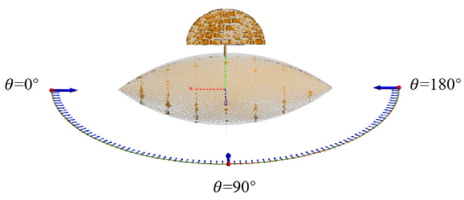
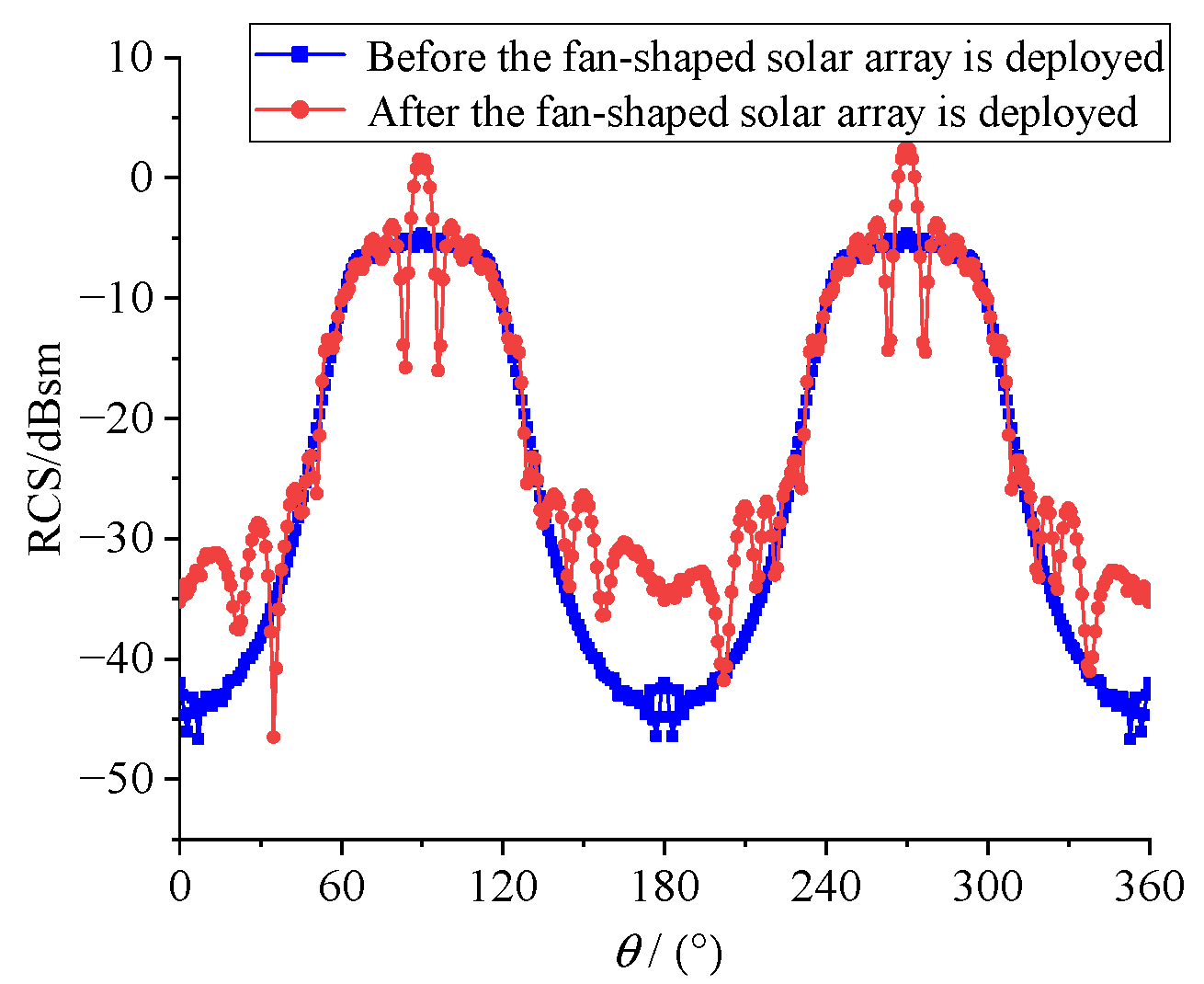
In order to study the RCS variation in the satellite before and after the sector solar array deployment, the schematic of the incident wave after the solar array deployment and the RCS comparison before and after the satellite solar array deployment are given in Figure 10 and Figure 11, respectively, with an incidence frequency of 4 GHz, VV polarization, and circumferential incidence.
After the deployment of the fan-shaped solar array, the backscattering becomes significantly stronger when the radar wave is vertically incident the combination of the solar array and the satellite, resulting in an increase in RCS from −4.63 dBm to 2.57 dBsm, an increase of 7.2 dBsm. In addition, RCS in the angular domain around 180° also rises to a certain extent, which is the contribution of specular reflection and edge diffraction of the solar array, and the RCS in the remaining angular domain basically overlaps. It can be seen that although the fan-shaped solar array increases the RCS in the small angle domain, the damage to the overall stealth performance of the satellite is small, and due to the covering of the solar array by the satellite, the ground-based radar wave within a certain angle range cannot be directly incident into the fan-shaped solar array, which has certain advantages over the traditional solar array in terms of configuration stealth.
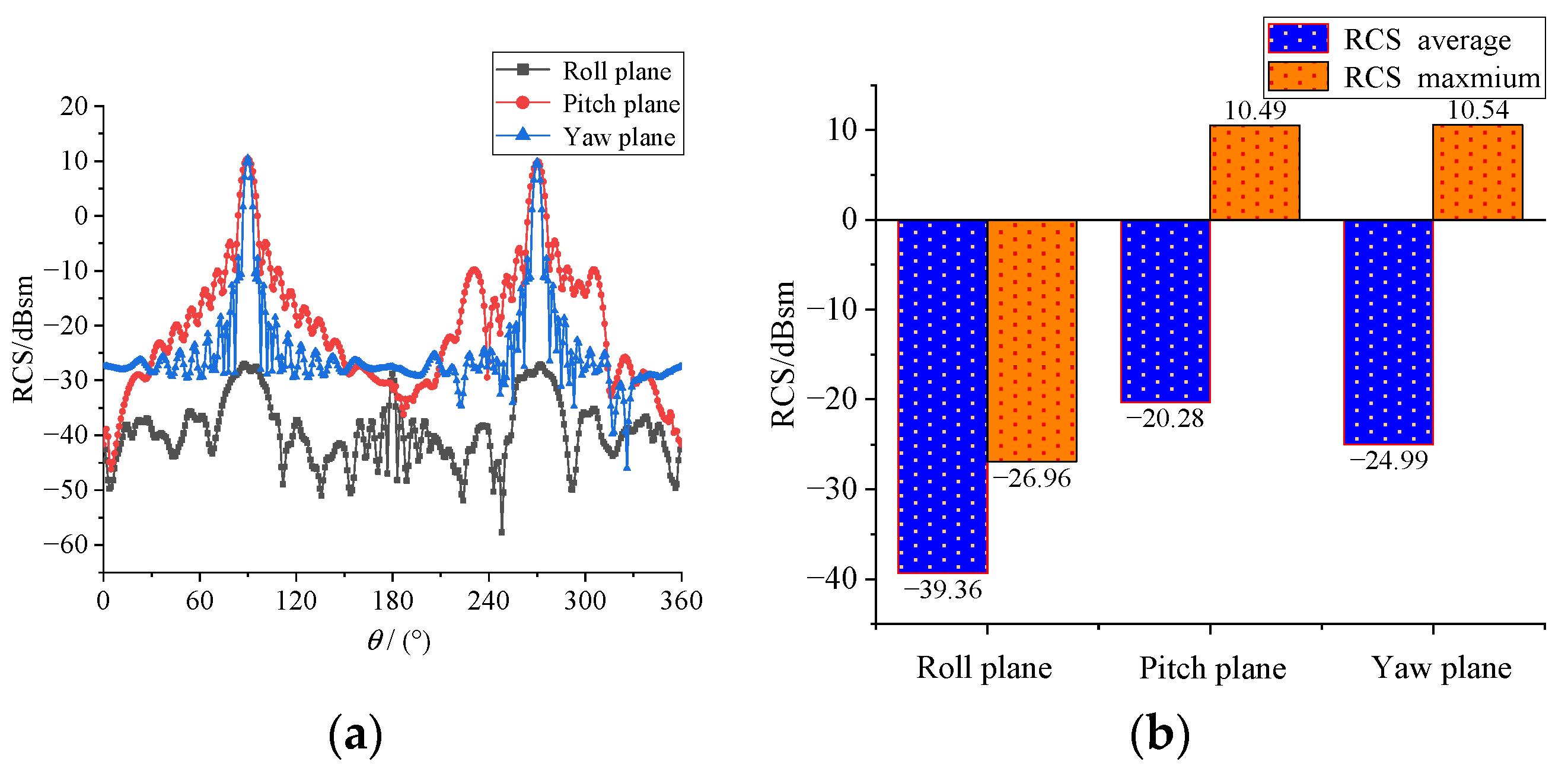
Figure 12 is a schematic diagram of the radar wave incident on the isolated solar array model from three typical azimuths. The three incident azimuths are the roll plane, the pitch plane, and the yaw plane.
Figure 13 shows the RCS distribution characteristics of the fan-shaped solar array on the roll plane, the pitch plane, and the yaw plane.
The RCS characteristics of the pitch and yaw planes are similar, the RCS of the two scattering main flaps (90 and 270°) are both 10.5 dBsm, and their RCS is mainly contributed to by the specular reflection from the solar array surface. The RCS of the roll plane is contributed to by the very weak specular reflection at the edge of the solar array and the creeping wave diffraction of the rotating axis; its overall RCS is below −30 dBsm and the average RCS value is only −39.36 dBsm, which is lower than that of the pitch and yaw planes by 19.08 dBsm and 14.37 dBsm, respectively. The RCS of the three typical detection azimuths is quite different, the stealth performance of the roll plane is the best, the yaw plane is the second, and the pitch plane is the worst.
The fan-shaped solar array can be rotated at any angle through the rotating shaft. Figure 14 shows the three-dimensional model of the satellite when the solar array rotates to three typical positions. In order to explore the influence of the solar array rotation angle on the satellite RCS characteristics, Figure 15 shows the comparison of satellite RCS characteristics under three different rotation angles.
The analysis of Figure 15a shows that the position of the main scattering flap of the RCS characteristic curve changes due to the change of the direction of the solar array specular reflection caused by the solar array rotation. In other words, when the solar array rotates by a certain angle, the RCS distribution curve of the satellite is shifted to the right by a certain angle, but this overall shift is not exactly “copied”, and there are still a few angular areas where the RCS is different. It can be seen from Figure 15b that the stealth performance of the satellite gradually decreases as the rotation angle increases. From the position of the solar array rotating 0° to the position of rotation 90°, the mean value of satellite RCS increases from −21.41 dBsm to −16.35 dBsm; the increase is 5.06 dBsm. Therefore, the stealth performance of the satellite configuration in Figure 14a is better than that in Figure 14b,c, and thus the satellite should keep the solar array in the attitude of Figure 14a as much as possible when it is in orbit.

4.4. Radar Maximum Detection Distance Analysis

The maximum detection distance of the radar is proportional to the fourth root of the target RCS, so reducing the target RCS can reduce the detection distance of the radar and reduce the probability of the target being detected by the radar. The probability of target detection by radar is closely related to the size of the target’s own RCS, the distance from the radar, and other factors. The calculation formula for the probability of target detection by Doppler radar search is:
P Dk = exp ( 9.5 Ω R S jk Δ θ a f r )
S jk = P t G 2 λ 2 E n σ ¯ ( 4 π ) 3 k b T 0 B n F n L n R T 4
where   P Dk is the probability of the radar finding the target, Ω R is the antenna scanning angular velocity, S jk is the individual pulse signal-to-noise ratio, Δ θ a is the radar horizontal flap width, f r is the radar pulse repetition frequency, P t is the radar transmit power, G is the antenna gain, σ ¯ is the arithmetic mean of the RCS, E n is the compression ratio of the pulse, k b is the Boltzmann constant with the value of 1.38 × 10⁻²³ W × s/K, T 0 is the standard room temperature 290 K, B n is the receiver noise bandwidth, F n   is the receiver noise factor, L n is the total system loss, and R T is the maximum distance at which a pulse Doppler radar can detect a target.
The relevant data of a pulse Doppler radar selected for the calculation in this section are shown in Table 4 [19,20].
During the orbital flight of the stealth satellite, its position and attitude change relative to the direction of the ground-based and space-based detection radar; the RCS will rise or decrease, and the maximum dangerous distance detected by the radar will also change accordingly. In this section, four different observation directions of stealth satellites are selected for the study.
Figure 16 gives the probability distribution of three stealth satellites being detected by a certain pulsed Doppler radar under the X-band (10 GHz) in the −30° ≤   θ   ≤ 30°, 150° ≤ θ   ≤ 210°, 60° ≤ θ   ≤ 120°, and 0° ≤ θ   ≤ 360°. The horizontal coordinates indicate the maximum distance that the radar can detect from our satellite, and the vertical coordinates indicate the probability of the satellite being detected by the radar.
As the radar detection distance decreases, the probability of a satellite being detected by radar increases, which means that the closer the radar is to the detected target within the maximum detection distance, the greater the probability of the target being detected. The maximum radar detection distance of Olive-B is the lowest, compared with the other two stealth satellites in the spaceward, groundward, and omnidirectional angular domains. All three stealth configurations (including Olive-A stealth and non-stealth attitudes) have a low probability of being detected by enemy radars; the maximum radar detection distance is below 20 km and the difference between the maximum radar detection distances of the three satellites is small. Unlike the other three detection directions, the maximum radar detection distance of TX-1 is the smallest in the lateral angle domain, and the radar detection distance of different stealth configurations of satellites varies greatly, especially given the maximum detection distance of non-stealth attitude of Olive-A configuration is significantly higher than the other three stealth satellites.
Figure 17 gives a comparison of the maximum radar detection distances of the three stealth satellites at a detection probability of 10% under the X-band radar (10 GHz), where the Olive-A configuration is only taken in its stealthy attitude. The maximum distances detected by radar in the spaceward, groundward, lateral, and omnidirectional directions for the Olive-B configuration are 58.68%, 46.59%, 98.17%, and 67.03% of those for the Olive-A configuration and 24.40%, 15.73%, 200.37%, and 58.35% of those for the TX-1, respectively. This indicates that the application of radar stealth technology can effectively reduce the maximum radar detection distance of the satellite and improve the satellite’s in-orbit survivability and operational effectiveness.
The maximum radar detection distance of the satellite is also closely related to the frequency size of the radar wave. In this section, six different frequencies of radar waves from L-band to Ku-band are selected to study the effect of frequency size on the maximum radar detection distance.
Figure 18 shows the probability distribution of three kinds of stealth satellites detected by the enemy radar detection system under the incidence of radar waves of different frequencies. Table 5 shows the comparison of the maximum detection distances of the three kinds of stealth satellites when the pulse Doppler radar finds the target with a probability of 10%. It can be seen that:
(1)
The probabilities of the three stealth satellites being detected by enemy radars at different frequencies are also quite different. Among them, the L-band has the highest probability of being detected by the radar, and the C, X, and Ku-bands have a higher probability of being detected by the radar.
(2)
The probability of different satellite stealth configurations being detected by radar is affected differently by the frequency. The probability of the multi-faceted stealth configuration (TX-1) being detected by radar will change significantly with the increase in frequency, while the two Olive configurations are less affected by frequency, especially the Olive-B configuration.
(3)
Under the irradiation of a certain pulse Doppler radar of six frequencies with a probability of finding a target of 10%, the radar maximum detection distance of TX-1 reaches a maximum of 61.91 km at 1 GHz (L-band), and at 10 GHz (X-band) the minimum value is 13.52 km. The radar maximum detection distance of the Olive-A configuration non-stealth attitude reaches a maximum value of 48.10 km at 1 GHz (L-band) and a minimum value of 9.28 km at 16 GHz (Ku-band). The radar maximum detection distance in the stealth attitude of Olive-A configuration reaches a maximum value of 40.95 km at 1 GHz (L-band) and a minimum value of 8.14 km at 13 GHz (Ku-band). The radar maximum detection range of the Olive-B configuration reaches a maximum of 24.80 km at 1 GHz (L-band) and a minimum of 6.27 km at 16 GHz (Ku-band). The radar maximum detection distance of the Olive-B obtained by configuration optimization is smaller than that of the other two stealth configurations in each frequency band, and it generally shows a downward trend with the increase in the incident wave frequency. To sum up, the stealth performance of satellites at high frequencies is better than that at low frequencies, which also shows that how to deal with threats from low-frequency and long-range early warning radars is the key to improving the in-orbit survivability of olive stealth satellites.

5. Conclusions

Based on the multi-faceted stealth configuration of the TX-1 satellite, this paper proposes an optimal design method for the stealth configuration of the satellite to improve the stealth performance of the satellite in orbit. Aiming at the two optimized stealth satellite configurations, a fan-shaped stealth solar array is designed, and the anechoic chamber RCS measurement is carried out on the metal model of Olive-B with better performance. Both its low scattering characteristics are verified and the correctness of the calculation method is demonstrated. In this paper, a large number of numerical simulations of stealth characteristics of various stealth satellites are carried out, and the following conclusions are obtained:
(1)
Under the same electrical size, the average RCS of the Olive configuration is significantly lower than that of the multifaceted stealth configuration, the number of scattering peaks is also lower, and the overall stealth performance is more prominent.
(2)
After the fan-shaped solar array is deployed, the RCS of the olivine satellite only increases to a certain extent in a few angular domains, and the RCS changes very little in most angular domains, which has little impact on the stealth performance of the satellite. When the rotation angle of the fan-shaped solar array is 0°, the mean and maximum value of satellite RCS reach the minimum.
(3)
The maximum radar detection distance of Olive-B configuration in each band is smaller than that of Olive-A and TX-1, and it generally declines with the increase in the incident frequencies. In terms of radar stealth performance, Olive-B is the best, followed by Olive-A, and TX-1 is the worst.

Author Contributions

Writing—original draft, H.S.; Writing—review & editing, Y.Q. All authors have read and agreed to the published version of the manuscript.

Funding

This research received no external funding.

Data Availability Statement

Not applicable.

Conflicts of Interest

The authors declare no conflict of interest.

References

  1. Huang, H. Concept study on satellite stealth. Aerosp. Electron. Warf. 2010, 6, 009. [Google Scholar]
  2. Wang, C.; Liao, W. Current status of stealth satellites and their applications in space offense and defense. Space Electron. Countermeas. 2011, 27, 17–19. [Google Scholar]
  3. Hu, H.; Zhang, X.; Liao, W.; Kong, X. Research progress and development trend of satellite stealth technology. J. Natl. Univ. Def. Technol. 2021, 43, 107–127. [Google Scholar]
  4. Zheng, K. Research on the Key Technology of Stealthy Microsatellite Structure Design; Nanjing University of Aeronautics and Astronautics: Nanjing, China, 2011. [Google Scholar]
  5. Sang, J. Stealth Technology of Flying Vehicles; Aviation Industry Press: Beijing, China, 2013. [Google Scholar]
  6. Morton, E.; Karl, H.; Richard, H. Satellite Signature Suppression Shield. U.S. Patent US5345238, 6 September 1994. [Google Scholar]
  7. Chung, S.; Chuang, Y. Simulation on change of generic satellite radar cross section via artificially created plasma sprays. Plasma Sources Sci. Technol. 2016, 25, 35–50. [Google Scholar] [CrossRef]
  8. Zhu, D.; Zhang, Z.; Zhao, C.; Liu, Y. A satellite configuration design to achieve optical stealth. Space Control Technol. Appl. 2017, 43, 61–66. [Google Scholar]
  9. Gong, J.; Ding, F. Study on the extraction of scattering characteristics of optical/infrared reconnaissance satellite targets. Infrared Laser Eng. 2017, 46, 193–198. [Google Scholar]
  10. Zhou, Z.; Huang, J.; Yi, M. Comprehensive optimization of aerodynamic noise and radar stealth for helicopter rotor based on pareto solution. Aerosp. Sci. Technol. 2018, 82–83, 607–619. [Google Scholar] [CrossRef]
  11. Xiao, H.; Liu, L.; Lv, M. Simulation of stealth characteristics of X-tail airship near space. J. Beijing Univ. Aeronaut. Astronaut. 2015, 41, 181–186. [Google Scholar]
  12. Qin, Y.; Sun, H.; Yue, X. Effect of coated radar absorbing materials on electromagnetic stealth performance of warplanes. J. Microwave J. 2021, 37, 249–252. [Google Scholar]
  13. Yue, K.; Liu, W.; Li, G. Numerical simulation of RCS for carrier electronic warfare airplanes. Chin. J. Aeronaut. 2015, 28, 545–555. [Google Scholar] [CrossRef] [Green Version]
  14. Zhou, Z.; Huang, J. Study of RCS characteristics of tilt-rotor aircraft based on dynamic calculation approach. Chin. J. Aeronaut. 2022, 35, 426–437. [Google Scholar]
  15. Zhou, Z.; Huang, J.; Wu, N. Acoustic and radar integrated stealth design for ducted tail rotor based on comprehensive optimization method. Aerosp. Sci. Technol. 2019, 92, 244–257. [Google Scholar] [CrossRef]
  16. Wu, A.; Wu, Y.; Yang, Y.; Zhang, N. The method of moments physical optics hybrid algorithm to calculate the electromagnetic scattering field of multiscale compound targets. Chin. J. Radio Sci. 2019, 34, 83–90. [Google Scholar]
  17. Zhao, W.; Li, J.; Hu, L. Efficient current-based hybrid analysis of wire antennas mounted on a large realistic aircraft. IEEE Trans. Antennas Propag. 2010, 58, 2666–2672. [Google Scholar] [CrossRef]
  18. Qin, Y.; Sun, H.; Yue, X. Stealthy configuration design and optimization analysis of microsatellite. J. Beijing Univ. Aeronaut. Astronaut. 2022, 48, 2102–2110. [Google Scholar]
  19. Yue, K. Static and Dynamic RCS Characteristics of Combat Aircraft; Beihang University Press: Beijing, China, 2016. [Google Scholar]
  20. Jiang, X. Integrated Optimization Design and Application of Helicopter Aerodynamic/Radar Stealth Characteristics; Nanjing University of Aeronautics and Astronautics: Nanjing, China, 2016. [Google Scholar]
Figure 1. Anechoic chamber test verification. (a) Schematic diagram of incident wave. (b) Comparison of test and simulation results.
Aerospace 09 00815 g001
Figure 2. Stealthy configuration optimization design of the satellite.
Aerospace 09 00815 g002
Figure 3. Two radar wave incident attitudes of Olive-A configuration. (a) Incident in non-stealth attitude. (b) Incident in stealth attitude.
Aerospace 09 00815 g003
Figure 4. Comparison of RCS in different attitudes of the Olive-A configuration. (a) Comparison of RCS distribution. (b) Comparison of mean and maximum values of RCS.
Aerospace 09 00815 g004
Figure 5. RCS distribution at 10 GHz for 4 satellite configurations.
Aerospace 09 00815 g005
Figure 6. RCS comparison of the stealth attitude of the Olive-A and the Olive-B. (a) Comparison of RCS distribution. (b) Comparison of RCS mean and maximum values.
Aerospace 09 00815 g006
Figure 7. RCS test of the Olive-B satellite. (a) Metal model of the Olive-B. (b) Anechoic chamber.
Aerospace 09 00815 g007
Figure 8. Comparison of RCS test and simulation results.
Aerospace 09 00815 g008
Figure 9. Three-dimensional model of the satellite after the deployment of the fan-shaped solar array.
Aerospace 09 00815 g009
Figure 10. The schematic of incident wave.
Aerospace 09 00815 g010
Figure 11. Comparison of RCS before and after the deployment of the fan-shaped solar array.
Aerospace 09 00815 g011
Figure 12. Schematic diagram of three incident orientations.
Aerospace 09 00815 g012
Figure 13. Comparison of RCS under three detection orientations. (a) RCS characteristic distribution; (b) RCS average and maximum.
Aerospace 09 00815 g013
Figure 14. Schematic diagram of solar array rotation angle. (a) 0°; (b) 45°; (c) 90°.
Aerospace 09 00815 g014
Figure 15. Comparison of RCS under different rotation angles. (a) RCS characteristic distribution; (b) RCS mean and maximum.
Aerospace 09 00815 g015
Figure 16. Detection probability of satellites under X-band radar. (a) Spaceward; (b) Groundward; (c) Lateral; (d) Omnidirectional.
Aerospace 09 00815 g016aAerospace 09 00815 g016b
Figure 17. Comparison of the maximum radar detection distances of the three stealth satellites. (a) Spaceward; (b) Groundward; (c) Lateral; (d) Omnidirectional.
Aerospace 09 00815 g017aAerospace 09 00815 g017b
Figure 18. Comparison of the comprehensive detection probability of three kinds of stealth satellites by radars with different frequencies. (a) TX-1; (b) non-stealthy attitude of the Olive-A; (c) stealthy attitude of the Olive-A; (d) Olive-B.
Aerospace 09 00815 g018
Table 1. In-orbit parameters of TX-1 stealth microsatellite.
Parameter ItemsLength/mWidth/mHeight/mIn-Orbit Quality/kgAltitude of the Orbit/kmType of Launch RocketsLocation of the Launch
Parameter Value0.6940.6080.99561495CZ-4BTaiyuan Satellite Launch Center
Table 2. Comparison of mean and maximum values of RCS at 10 GHz for 4 satellites.
Satellite ConfigurationsRCS Mean Values /dBsmRCS Maximum Values /dBsm
TX-1−20.1931.32
Eight-sided pointed cone−21.05−7.01
Ten-sided pointed cone−22.30−10.06
Olive-A−23.84−12.65
Table 3. In-orbit parameters of TX-1 stealthy microsatellite.
Parameter ItemsLength/mWidth/mHeight/mDistance
between
Antenna and Target/m
Antenna Gain/dBAntenna Flap Width/°Antenna Aperture/m
Parameter Value0.820.300.303.512.938.25°0.12
Table 4. Relevant data of a pulse Doppler radar.
Parameter ItemParameter Value
Δ θ a (°)7
f r 300
Ω R (°/s)30
P t (MW)1
G (dB)36
E n 900
B n (MHz)0.077
F n (dB)55
L n (dB)20
Table 5. Comparison of the radar maximum detection distance of satellites with a 10% probability of detection of the target.
f/GHzRadar Maximum Detection Distance /km
TX-1Non-Stealthy
Attitude of the Olive-A
Stealthy Attitude of the Olive-AOlive-B
1 GHz61.9148.1040.9524.80
4 GHz22.9126.3123.9819.51
7 GHz15.4314.0711.319.94
10 GHz13.5212.9511.157.91
13 GHz14.1510.238.147.15
16 GHz17.839.288.936.27
Publisher’s Note: MDPI stays neutral with regard to jurisdictional claims in published maps and institutional affiliations.

